A Parametric Non-Convex Decomposition Algorithm for Real-Time and Distributed NMPC

Jean-Hubert Hours,  and Colin N. Jones
Abstract

A novel decomposition scheme to solve parametric non-convex programs as they arise in Nonlinear Model Predictive Control (NMPC) is presented. It consists of a fixed number of alternating proximal gradient steps and a dual update per time step. Hence, the proposed approach is attractive in a real-time distributed context. Assuming that the Nonlinear Program (NLP) is semi-algebraic and that its critical points are strongly regular, contraction of the sequence of primal-dual iterates is proven, implying stability of the sub-optimality error, under some mild assumptions. Moreover, it is shown that the performance of the optimality-tracking scheme can be enhanced via a continuation technique. The efficacy of the proposed decomposition method is demonstrated by solving a centralised NMPC problem to control a DC motor and a distributed NMPC program for collaborative tracking of unicycles, both within a real-time framework. Furthermore, an analysis of the sub-optimality error as a function of the sampling period is proposed given a fixed computational power.

Index Terms:
Augmented Lagrangian, Alternating minimisation, Proximal gradient, Strong regularity, Kurdyka-Lojasiewicz property, Nonlinear Model Predictive Control.
footnotetext: Jean-Hubert Hours and Colin N. Jones are with the Laboratoire d’Automatique, Ecole Polytechnique Fédérale de Lausanne (EPFL), CH-101510151015 Lausanne (e-mail:jean-hubert.hours@epfl.ch,colin.jones@epfl.ch).
The work of Jean-Hubert Hours is supported by the Swiss National Science Foundation (SNSF) under grant 200021200021200021-135218135218135218. The work of Colin N. Jones is supported by the European Research Council under the European Union’s Seventh Framework Programme (FP/200720072007-201320132013), ERC Grant Agreement 307608307608307608.

I Introduction

The applicability of NMPC to fast and complex dynamics is hampered by the fact that an NLP, which is generally non-convex, is to be solved at every sampling time. Solving an NLP to full accuracy is not tractable when the system’s sampling frequency is high, which is the case for many mechanical or electrical systems. This difficulty is enhanced when dealing with distributed systems, which consist of several sub-systems coupled through their dynamics, objectives or constraints. This class of systems typically lead to large-scale NLPs, which are to be solved online as the system evolves. Solving such programs in a centralised manner may be computationally too demanding and may also hamper autonomy of the agents. Therefore, much research effort is currently brought to develop decentralised computational methods applicable to MPC. Although several distributed linear MPC algorithms are now available, there only exists very few strategies [24, 16] that can address online distributed NMPC programs, as they generally result in non-convex problems. Most of these techniques essentially consist in fully convexifying the problem at hand and resort to Sequential Convex Programming (SCP). Hence, from a theoretical point of view, they cannot be fully considered as distributed non-convex techniques, since the decomposition step occurs at the convex level. In addition, the SCP methods of [24, 16] have not been analysed in an online optimisation framework, where fixing the number of iterations is critical. In general, it should be expected that SCP techniques require a high number communications between agents, since a sequence of distributed convex NLPs is to be solved. Therefore, our main objective is to propose a novel online distributed optimisation strategy for solving NMPC problems in a real-time framework. Our approach is useful for deployment of NMPC controllers, but can also be applied in the very broad parametric optimisation context. We address the problem of real-time distributed NMPC from a distributed optimisation perspective. However, some approaches based on distributed NMPC algorithms, which fully decompose the NMPC problem into smaller NMPC problems exist in the literature [18, 30]. Yet, to the author’s knowledge, they have not been analysed in a real-time setting. Besides, the approach of [30] is limited to the input constrained case.

A standard way of solving distributed NLPs is to apply Lagrangian decomposition [10]. This technique requires strong duality, which is guaranteed by Slater’s condition in the convex case, but rarely holds in a non-convex setting. The augmented Lagrangian framework [7] mitigates this issue by closing the duality gap for properly chosen penalty parameters [28]. The combination of the bilinear Lagrangian term with the quadratic penalty also turns out to be computationally more efficient than standard penalty approaches, as the risk of running into ill-conditioning is reduced by the fast convergence of the dual sequence. In addition, global convergence of the dual iterates can be obtained, as in the lancelot package [11, 12]. However, the quadratic penalty term induces non-separability in the objective, which hampers decomposing the NLP completely. Several approaches have been proposed to remedy this issue [21]. Taking inspiration from the Alternating Direction Method of Multipliers (ADMM) [10], which has recently gained in popularity, even in a non-convex setting (yet without convergence guarantees) [23], we propose addressing the non-separability issue via a novel Block-Coordinate Descent (BCD) type technique. BCD or alternating minimisation strategies are known to lead to ‘easily’ solvable sub-problems, which can be parallelised under some assumptions on the coupling, and are well-suited to distributed computing platforms [8]. BCD-type techniques are currently raising interest for solving very large-scale programs [25]. Until very recently, for non-convex objectives with certain structure, convergence of the BCD iterates was proven in terms of limit points only [32]. The central idea of our algorithm is to apply a truncated proximal alternating linearised minimisation in order to solve the primal augmented Lagrangian problem approximately. Our convergence analysis is based on the recent results of [4, 6], which provide a very general framework for proving global convergence of descent methods on non-smooth semi-algebraic objectives.

Augmented Lagrangian techniques have proven effective at solving large-scale NLPs [35]. Yet, in an online context, they are hampered by the fact that a sequence of non-convex programs need to be solved to an increasing level of accuracy [7]. Recently, a parametric augmented Lagrangian algorithm has been introduced by [34] for centralised NMPC problems.  Our online decomposition method builds upon the ideas of [34], but extends them to the online distributed framework, which requires a significantly different approach. Furthermore, our analysis brings the results of [34] one step further by proving contraction of the sequence of primal-dual iterates under some mild assumptions. In particular, new insights are given on how the penalty parameter and the number of primal iterations need to be tuned in order to ensure boundedness of the tracking error, which is the core of the analysis of a parametric optimisation algorithm. Moreover, an interesting aspect of our analysis is that it shows how the proposed decomposition algorithm can be efficiently modified via a continuation, or homotopy, strategy [3], leading to faster convergence of the tracking scheme. This theoretical observation is confirmed by a numerical example presented later in the paper. Our technique is also designed to handle a more general class of parametric NLPs, where the primal Projected Successive Over-Relaxation (PSOR) of [34] is limited to quadratic objectives subject to non-negativity constraints.

From an MPC perspective, the effect of the sampling period on the behaviour of the combined system-optimiser dynamics has been analysed in a few studies [1, 2]. However, it is often claimed that faster sampling rates lead to better closed-loop performance. This thinking neglects the fact that MPC is an optimisation-based control strategy, which requires a significant amount of computations within a sampling interval. Hence, sampling faster entails reducing the number of iterations in the optimiser quite significantly, as the computational power of any computing platform is limited, especially in the case of embedded or distributed applications. In the last part of the paper, we propose an analysis of the effect of the sampling period on the behaviour of the system in closed-loop with our parametric decomposition strategy. It is demonstrated that the proposed theory accounts for the observed numerical behaviour quite nicely. In particular, tuning the penalty parameter of the augmented Lagrangian turns out to significantly improve the tracking performance at a given sampling period.

In Section III, the parametric distributed optimisation scheme is presented. In Section IV, some key theoretical ingredients such as strong regularity of generalised equations and the Kurdyka-Lojasiewicz inequality are introduced, and convergence of the primal sequence is proven. As explained later in the paper, strong regularity and the Kurdyka-Lojasiewicz inequality encompass a broad class of problems encountered in practice. Then, in Section V, contraction of the primal-dual sequence is proven and conditions ensuring stability of the tracking error are derived. In Section VI, basic computational aspects are investigated. Finally, the proposed approach is tested on two numerical examples, which consist in controlling the speed of a DC motor to track a piecewise constant reference for the first one, and collaborative tracking of unicycles for the second one. The effect of the sampling period on the tracking error, passed through the system dynamics, is analysed given a fixed computational power, or communication rate for the distributed case.

II Background

Definition 1 (Proximal operator).

Let f:n{+}:𝑓superscript𝑛f:\mathbb{R}^{n}\rightarrow\mathbb{R}\cup\left\{+\infty\right\} be a proper lower-semicontinuous function and α>0𝛼0\alpha>0. The proximal operator of f𝑓f with coefficient α𝛼\alpha, denoted by proxαf()subscriptsuperscriptprox𝑓𝛼\operatorname{prox}^{f}_{\alpha}\left(\cdot\right), is defined as follows:

proxαf(x):=argminyf(y)+α2yx22.assignsubscriptsuperscriptprox𝑓𝛼𝑥subscriptargmin𝑦𝑓𝑦𝛼2superscriptsubscriptnorm𝑦𝑥22\displaystyle\operatorname{prox}^{f}_{\alpha}\left(x\right):=\operatorname{argmin}_{y}f(y)+\displaystyle\frac{\alpha}{2}\left\|y-x\right\|_{2}^{2}\enspace. (1)
Definition 2 (Critical point).

Let f𝑓f be a proper lower semicontinuous function. A necessary condition for xsuperscript𝑥x^{\ast} to be a minimiser of f𝑓f is that

0f(x),0𝑓superscript𝑥\displaystyle 0\in\partial f\left(x^{\ast}\right)\enspace, (2)

where f(x)𝑓superscript𝑥\partial f\left(x^{\ast}\right) is the sub-differential of f𝑓f at xsuperscript𝑥x^{\ast} [29].

Points satisfying (2) are called critical points.

Definition 3 (Normal cone to a convex set).

Let ΩΩ\Omega be a convex set in nsuperscript𝑛\mathbb{R}^{n} and x¯Ω¯𝑥Ω\bar{x}\in\Omega. The normal cone to ΩΩ\Omega at x¯¯𝑥\bar{x} is the set

𝒩Ω(x¯):={vn|xΩ,v(xx¯)0}.assignsubscript𝒩Ω¯𝑥conditional-set𝑣superscript𝑛formulae-sequencefor-all𝑥Ωsuperscript𝑣top𝑥¯𝑥0\displaystyle\mathcal{N}_{\Omega}\left(\bar{x}\right):=\left\{v\in\mathbb{R}^{n}~{}\big{|}~{}\forall x\in\Omega,v^{\scriptscriptstyle\top}\left(x-\bar{x}\right)\leq 0\right\}\enspace. (3)

The indicator function of a closed subset ΩΩ\Omega of nsuperscript𝑛\mathbb{R}^{n} is denoted by ιΩsubscript𝜄Ω\iota_{\Omega} and is defined as

ιΩ(x)={0if xΩ+if xΩ.subscript𝜄Ω𝑥cases0if 𝑥Ωif 𝑥Ω\displaystyle\iota_{\Omega}\left(x\right)=\begin{cases}0&\mbox{if }x\in\Omega\\ +\infty&\mbox{if }x\notin\Omega\end{cases}\enspace. (4)
Lemma 1 (Sub-differential of indicator function [29]).

Given a convex set ΩΩ\Omega, for all xΩ𝑥Ωx\in\Omega,

ιΩ(x)=𝒩Ω(x).subscript𝜄Ω𝑥subscript𝒩Ω𝑥\displaystyle\partial\iota_{\Omega}\left(x\right)=\mathcal{N}_{\Omega}\left(x\right)\enspace. (5)
Lemma 2 (Descent lemma,[7]).

Let L:n:𝐿superscript𝑛L:\mathbb{R}^{n}\rightarrow\mathbb{R} a continuously differentiable function such that its gradient L𝐿{\nabla}L is λLsubscript𝜆𝐿\lambda_{L}-Lipschitz continuous. For all x,yn𝑥𝑦superscript𝑛x,y\in\mathbb{R}^{n},

L(y)L(x)+L(x)(yx)+λL2yx22.𝐿𝑦𝐿𝑥𝐿superscript𝑥top𝑦𝑥subscript𝜆𝐿2superscriptsubscriptnorm𝑦𝑥22\displaystyle L(y)\leq L(x)+{\nabla}L(x)^{\scriptscriptstyle\top}\left(y-x\right)+\displaystyle\frac{\lambda_{L}}{2}\left\|y-x\right\|_{2}^{2}\enspace. (6)

The distance of a point xn𝑥superscript𝑛x\in\mathbb{R}^{n} to a subset ΣΣ\Sigma of nsuperscript𝑛\mathbb{R}^{n} is defined by

d(x,Σ):=infyΣxy2.assign𝑑𝑥Σsubscriptinf𝑦Σsubscriptnorm𝑥𝑦2\displaystyle d(x,\Sigma):=\operatorname*{inf}_{y\in\Sigma}\big{\|}x-y\big{\|}_{2}\enspace. (7)

The open ball with center x𝑥x and radius r𝑟r is denoted by (x,r)𝑥𝑟\mathcal{B}\left(x,r\right). Given x¯,x¯n¯𝑥¯𝑥superscript𝑛\underline{x},\overline{x}\in\mathbb{R}^{n}, the box set {xn|x¯xx¯}conditional-set𝑥superscript𝑛¯𝑥𝑥¯𝑥\left\{x\in\mathbb{R}^{n}~{}\big{|}~{}\underline{x}\leq x\leq\overline{x}\right\} is denoted by B(x¯,x¯)𝐵¯𝑥¯𝑥B\left(\underline{x},\overline{x}\right). Given a closed convex set ΩnΩsuperscript𝑛\Omega\subseteq\mathbb{R}^{n}, the single-valued projection onto ΩΩ\Omega is denoted by πΩ()subscript𝜋Ω\pi_{\Omega}\left(\cdot\right). The relative interior of ΩnΩsuperscript𝑛\Omega\subseteq\mathbb{R}^{n} is denoted by riΩriΩ\operatorname{ri}\Omega. Given a polynomial function f𝑓f, its degree is denoted by deg(f)degree𝑓\deg\left(f\right). A semi-algebraic function is a function whose graph can be expressed as a union of intersections of level sets of polynomials.

III Solving time-dependent distributed nonlinear programs

III-A Problem formulation

The following class of parametric NLPs with separable cost, partially separable equality constraints and separable inequality constraints is considered

minimisez1,,zNaJ(z):=i=1NaJi(zi)assignsubscriptminimisesubscript𝑧1subscript𝑧subscript𝑁𝑎𝐽𝑧superscriptsubscript𝑖1subscript𝑁𝑎subscript𝐽𝑖subscript𝑧𝑖\displaystyle\operatorname*{minimise}_{z_{1},\ldots,z_{N_{a}}}~{}J\left(z\right):=\sum_{i=1}^{N_{a}}J_{i}\left(z_{i}\right) (8)
s.t.Qc(z1,,zNa)=0,s.t.subscript𝑄𝑐subscript𝑧1subscript𝑧subscript𝑁𝑎0\displaystyle\text{s.t.}~{}~{}~{}~{}Q_{c}\left(z_{1},\ldots,z_{N_{a}}\right)=0,\enspace
gi(zi)+Tisk=0,subscript𝑔𝑖subscript𝑧𝑖subscript𝑇𝑖subscript𝑠𝑘0\displaystyle~{}~{}~{}~{}~{}~{}~{}~{}g_{i}\left(z_{i}\right)+T_{i}s_{k}=0,\enspace
zi𝒵i,i{1,,Na},formulae-sequencesubscript𝑧𝑖subscript𝒵𝑖𝑖1subscript𝑁𝑎\displaystyle~{}~{}~{}~{}~{}~{}~{}~{}z_{i}\in\mathcal{Z}_{i},~{}i\in\left\{1,\ldots,N_{a}\right\},\enspace

where z:=(z1,,zNa)nzassign𝑧superscriptsuperscriptsubscript𝑧1topsuperscriptsubscript𝑧subscript𝑁𝑎toptopsuperscriptsubscript𝑛𝑧z:=\left(z_{1}^{\scriptscriptstyle\top},\ldots,z_{N_{a}}^{\scriptscriptstyle\top}\right)^{\scriptscriptstyle\top}\in\mathbb{R}^{n_{z}}, with nz=i=1Nani2subscript𝑛𝑧superscriptsubscript𝑖1subscript𝑁𝑎subscript𝑛𝑖2n_{z}=\sum_{i=1}^{N_{a}}n_{i}\geq 2 and zinisubscript𝑧𝑖superscriptsubscript𝑛𝑖z_{i}\in\mathbb{R}^{n_{i}}. The vectors zisubscript𝑧𝑖z_{i} model different agents, while the function Qc:nzm:subscript𝑄𝑐superscriptsubscript𝑛𝑧superscript𝑚Q_{c}:\mathbb{R}^{n_{z}}\rightarrow\mathbb{R}^{m} represent constraint couplings.

Remark 1.

For clarity, the definition of NLP (8) is restricted to constraint couplings. However, cost couplings can be addressed by the approach described in the sequel.

The functions Ji:ni:subscript𝐽𝑖superscriptsubscript𝑛𝑖J_{i}:\mathbb{R}^{n_{i}}\rightarrow\mathbb{R} and gi:nzqi:subscript𝑔𝑖superscriptsubscript𝑛𝑧superscriptsubscript𝑞𝑖g_{i}:\mathbb{R}^{n_{z}}\rightarrow\mathbb{R}^{q_{i}} are individual cost and constraint functionals at agent i{1,,Na}𝑖1subscript𝑁𝑎i\in\left\{1,\ldots,N_{a}\right\}. In an NMPC context, the nonlinear equality constraint involving gisubscript𝑔𝑖g_{i} models the dynamics of agent i𝑖i over a prediction horizon. The vector sksubscript𝑠𝑘s_{k} is a time-dependent parameter, which lies within a set 𝒮p𝒮superscript𝑝\mathcal{S}\subseteq\mathbb{R}^{p}, where k𝑘k stands for a time index. When it comes to NMPC, the parameter sksubscript𝑠𝑘s_{k} stands for a state estimate or a reference trajectory, for instance. The matrices Tiqi×psubscript𝑇𝑖superscriptsubscript𝑞𝑖𝑝T_{i}\in\mathbb{R}^{q_{i}\times{}p} are constant. The linear dependence of the local equality constraints in the parameter s𝑠s is not restrictive, as extra variables can be introduced in order to obtain this formulation. For all s𝒮𝑠𝒮s\in\mathcal{S}, we define the equality constraints functional

G(,s):=(Qc(),(g1()+T1s),,(gNa()+TNas))assign𝐺𝑠superscriptsubscript𝑄𝑐superscripttopsuperscriptsubscript𝑔1subscript𝑇1𝑠topsuperscriptsubscript𝑔subscript𝑁𝑎subscript𝑇subscript𝑁𝑎𝑠toptop\displaystyle G(\cdot,s):=\left(Q_{c}\left(\cdot\right)^{\scriptscriptstyle\top},\left(g_{1}\left(\cdot\right)+T_{1}s\right)^{\scriptscriptstyle\top},\ldots,\left(g_{N_{a}}\left(\cdot\right)+T_{N_{a}}s\right)^{\scriptscriptstyle\top}\right)^{\scriptscriptstyle\top}

For all i{1,,Na}𝑖1subscript𝑁𝑎i\in\left\{1,\ldots,N_{a}\right\}, the constraint sets 𝒵isubscript𝒵𝑖\mathcal{Z}_{i} are assumed to be bounded boxes. Note that such an assumption is not restrictive, as slack variables can always be introduced. KKT points of NLP (8) are denoted by wksuperscriptsubscript𝑤𝑘w_{k}^{\ast} or w(sk)superscript𝑤subscript𝑠𝑘w^{\ast}\left(s_{k}\right) without distinction.

Assumption 1.

The functions Qcsubscript𝑄𝑐Q_{c}, Jisubscript𝐽𝑖J_{i} and gisubscript𝑔𝑖g_{i} are multivariate polynomials. For each i{1,,Na}𝑖1subscript𝑁𝑎i\in\left\{1,\ldots,N_{a}\right\}, deg(Ji)2degreesubscript𝐽𝑖2\deg\left(J_{i}\right)\geq 2.

Remark 2.

From a control perspective, this implies that the theoretical developments that follow are valid when NLP (8) is obtained via discretisation of optimal control problems with polynomial dynamics and quadratic costs for instance.

As we are targeting distributed applications, further assumptions are required on the coupling function Qcsubscript𝑄𝑐Q_{c}.

Assumption 2 (Sparse coupling,[8]).

The sub-variables z1,,zNasubscript𝑧1subscript𝑧subscript𝑁𝑎z_{1},\ldots,z_{N_{a}} can be re-ordered and grouped together in such a way that a Gauss-Seidel sweep on the real-valued function Qc22superscriptsubscriptnormsubscript𝑄𝑐22\left\|Q_{c}\right\|_{2}^{2} can be performed in P𝑃P parallel steps, where PNamuch-less-than𝑃subscript𝑁𝑎P\ll N_{a}. The re-ordered and grouped sub-variables are denoted by z1,,zPsubscript𝑧1subscript𝑧𝑃z_{1},\ldots,z_{P}, so that the re-arranged vector z𝑧z is defined by z=(z1,,zP)𝑧superscriptsuperscriptsubscript𝑧1topsuperscriptsubscript𝑧𝑃toptopz=\left(z_{1}^{\scriptscriptstyle\top},\ldots,z_{P}^{\scriptscriptstyle\top}\right)^{\scriptscriptstyle\top}. In the remainder, it is assumed that NLP (8) has been re-arranged accordingly.

Remark 3.

Assumption 2 is standard in distributed computations [8]. It encompasses a large number of practical problems of interest. For consensus problems, in which coupling constraints z1zi=0subscript𝑧1subscript𝑧𝑖0z_{1}-z_{i}=0 appear for all i{2,,Na}𝑖2subscript𝑁𝑎i\in\left\{2,\ldots,N_{a}\right\}, one obtains P=2𝑃2P=2 parallel steps, corresponding to the update of z1subscript𝑧1z_{1} followed by the updates of z2,,zNasubscript𝑧2subscript𝑧subscript𝑁𝑎z_{2},\ldots,z_{N_{a}} in parallel. When the coupling graph is a tree, such as in the case of a distribution network, one also obtain P=2𝑃2P=2. Our approach is likely to be more efficient when P𝑃P is small relative to Nasubscript𝑁𝑎N_{a}.

III-B A non-convex decomposition scheme for optimality tracking

At every time instant k𝑘k, a critical point of the parametric NLP (8) is computed inexactly in a distributed manner. The key idea is to track time-dependent optima wksubscriptsuperscript𝑤𝑘w^{\ast}_{k} of (8) by approximately computing saddle points of the augmented Lagrangian

Lρ(z,μ,sk):=assignsubscript𝐿𝜌𝑧𝜇subscript𝑠𝑘absent\displaystyle L_{\rho}\left(z,\mu,s_{k}\right):=~{} J(z)+(μ+ρ2G(z,sk))G(z,sk),𝐽𝑧superscript𝜇𝜌2𝐺𝑧subscript𝑠𝑘top𝐺𝑧subscript𝑠𝑘\displaystyle J\left(z\right)+\left(\mu+\displaystyle\frac{\rho}{2}G\left(z,s_{k}\right)\right)^{\scriptscriptstyle\top}G\left(z,s_{k}\right)\enspace, (9)

subject to z𝒵𝑧𝒵z\in\mathcal{Z}, where 𝒵:=𝒵1×𝒵2××𝒵Passign𝒵subscript𝒵1subscript𝒵2subscript𝒵𝑃\mathcal{Z}:=\mathcal{Z}_{1}\times\mathcal{Z}_{2}\times\ldots\times\mathcal{Z}_{P} and μ:=(μC,μ1,,μP)m+qassign𝜇superscriptsuperscriptsubscript𝜇𝐶topsuperscriptsubscript𝜇1topsuperscriptsubscript𝜇𝑃toptopsuperscript𝑚𝑞\mu:=\left(\mu_{C}^{\scriptscriptstyle\top},\mu_{1}^{\scriptscriptstyle\top},\ldots,\mu_{P}^{\scriptscriptstyle\top}\right)^{\scriptscriptstyle\top}\in\mathbb{R}^{m+q}, with q:=i=1Pqiassign𝑞superscriptsubscript𝑖1𝑃subscript𝑞𝑖q:=\sum_{i=1}^{P}q_{i}, is a dual variable associated with the equality constraints Qc(z)=0subscript𝑄𝑐𝑧0Q_{c}\left(z\right)=0, g1(z1)+T1sk=0subscript𝑔1subscript𝑧1subscript𝑇1subscript𝑠𝑘0g_{1}\left(z_{1}\right)+T_{1}s_{k}=0,…, gP(zP)+TPsk=0subscript𝑔𝑃subscript𝑧𝑃subscript𝑇𝑃subscript𝑠𝑘0g_{P}\left(z_{P}\right)+T_{P}s_{k}=0. The scalar ρ>0𝜌0\rho>0 is the so-called penalty parameter, which remains constant as sksubscript𝑠𝑘s_{k} and μ𝜇\mu vary. As Qcsubscript𝑄𝑐Q_{c}, Jisubscript𝐽𝑖J_{i} and gisubscript𝑔𝑖g_{i} are multivariate polynomials, Lρ(,μ,s)subscript𝐿𝜌𝜇𝑠L_{\rho}\left(\cdot,\mu,s\right) is a multivariate polynomial, whose degree is assumed to be larger than 222. We define

dL:=deg(Lρ(,μ,s))2.assignsubscript𝑑𝐿degreesubscript𝐿𝜌𝜇𝑠2\displaystyle d_{L}:=\deg\left(L_{\rho}\left(\cdot,\mu,s\right)\right)\geq{2}\enspace. (10)

In the rest of the paper, sub-optimality of a variable is highlighted by a ¯¯\bar{\cdot}, and criticality by a superscript{\cdot}^{\ast}. We intend to build an approximate KKT point (z¯(sk+1),μ¯(sk+1))superscript¯𝑧superscriptsubscript𝑠𝑘1top¯𝜇superscriptsubscript𝑠𝑘1toptop\left(\bar{z}(s_{k+1})^{\scriptscriptstyle\top},\bar{\mu}(s_{k+1})^{\scriptscriptstyle\top}\right)^{\scriptscriptstyle\top} of (8) by incremental improvement from the KKT point (z¯(sk),μ¯(sk))superscript¯𝑧superscriptsubscript𝑠𝑘top¯𝜇superscriptsubscript𝑠𝑘toptop\left(\bar{z}(s_{k})^{\scriptscriptstyle\top},\bar{\mu}(s_{k})^{\scriptscriptstyle\top}\right)^{\scriptscriptstyle\top}, once the parameter sk+1subscript𝑠𝑘1s_{k+1} is available.

Algorithm 1 Optimality tracking splitting algorithm
Input: Suboptimal primal-dual solution (z¯(sk),μ¯(sk))superscript¯𝑧superscriptsubscript𝑠𝑘top¯𝜇superscriptsubscript𝑠𝑘toptop\left(\bar{z}(s_{k})^{\scriptscriptstyle\top},\bar{\mu}(s_{k})^{\scriptscriptstyle\top}\right)^{\scriptscriptstyle\top}, parameter sk+1subscript𝑠𝑘1s_{k+1}, augmented Lagrangian Lρ(,μ¯k,sk+1)subscript𝐿𝜌subscript¯𝜇𝑘subscript𝑠𝑘1{L_{\rho}\left(\cdot,\bar{\mu}_{k},s_{k+1}\right)}.
Primal/Inner loop:
z(0)z¯(sk)superscript𝑧0¯𝑧subscript𝑠𝑘z^{(0)}\leftarrow\bar{z}(s_{k})
for l=0M1𝑙0𝑀1l=0\ldots M-1 do
     for i=1P𝑖1𝑃i=1\ldots P do \triangleright PNamuch-less-than𝑃subscript𝑁𝑎P\ll N_{a}
         \triangleright In parallel in group i𝑖i
         zi(l+1)bckMin(zi(l),μ¯(sk),ρ,sk+1)superscriptsubscript𝑧𝑖𝑙1bckMinsuperscriptsubscript𝑧𝑖𝑙¯𝜇subscript𝑠𝑘𝜌subscript𝑠𝑘1z_{i}^{(l+1)}\leftarrow\texttt{bckMin}\left(z_{i}^{(l)},\bar{\mu}(s_{k}),\rho,s_{k+1}\right)
     end for
end for
z¯(sk+1)z(M)¯𝑧subscript𝑠𝑘1superscript𝑧𝑀\bar{z}(s_{k+1})\leftarrow z^{(M)}
Dual updateμ¯(sk+1)μ¯(sk)+ρG(z¯(sk+1),sk+1)¯𝜇subscript𝑠𝑘1¯𝜇subscript𝑠𝑘𝜌𝐺¯𝑧subscript𝑠𝑘1subscript𝑠𝑘1\bar{\mu}(s_{k+1})\leftarrow\bar{\mu}(s_{k})+{\rho}G\left(\bar{z}(s_{k+1}),s_{k+1}\right)

Algorithm 1 computes a suboptimal primal variable z¯(sk+1)¯𝑧subscript𝑠𝑘1\bar{z}(s_{k+1}) by applying M𝑀M iterations of a proximal alternating linearised method to minimise the augmented Lagrangian functional Lρ(,μ¯(sk),sk+1)+i=1Pι𝒵i()subscript𝐿𝜌¯𝜇subscript𝑠𝑘subscript𝑠𝑘1superscriptsubscript𝑖1𝑃subscript𝜄subscript𝒵𝑖L_{\rho}\left(\cdot,\bar{\mu}(s_{k}),s_{k+1}\right)+\sum_{i=1}^{P}\iota_{\mathcal{Z}_{i}}\left(\cdot\right).

We define the block-wise augmented Lagrangian function at group i{1,,P}𝑖1𝑃i\in\left\{1,\ldots,P\right\}, where PNamuch-less-than𝑃subscript𝑁𝑎P\ll N_{a} by Assumption 2,

Lρ,μ,s(i):=Lρ(z1,,zi1,,zi+1,,zP,μ,s)assignsuperscriptsubscript𝐿𝜌𝜇𝑠𝑖subscript𝐿𝜌subscript𝑧1subscript𝑧𝑖1subscript𝑧𝑖1subscript𝑧𝑃𝜇𝑠\displaystyle L_{\rho,\mu,s}^{(i)}:=L_{\rho}\left(z_{1},\ldots,z_{i-1},\cdot,z_{i+1},\ldots,z_{P},\mu,s\right) (11)

and a quadratic model at zisubscript𝑧𝑖z_{i}, encompassing all agents of group i𝑖i, given a curvature coefficient ci>0subscript𝑐𝑖0c_{i}>0,

q(;zi,ci):=assign𝑞subscript𝑧𝑖subscript𝑐𝑖absent\displaystyle q\left(\cdot;z_{i},c_{i}\right):= Lρ,μ,s(i)(zi)+Lρ,μ,s(i)(zi)(zi)\displaystyle L_{\rho,\mu,s}^{(i)}\left(z_{i}\right)+{\nabla}L_{\rho,\mu,s}^{(i)}\left(z_{i}\right)^{\scriptscriptstyle\top}\left(\cdot-z_{i}\right)
+ci2zi22.\displaystyle~{}~{}~{}~{}~{}~{}~{}~{}~{}~{}~{}~{}~{}~{}~{}~{}~{}~{}~{}~{}~{}~{}~{}~{}~{}~{}~{}~{}~{}~{}~{}+\displaystyle\frac{c_{i}}{2}\left\|\cdot-z_{i}\right\|_{2}^{2}\enspace.

Given an iteration index l1𝑙1l\geq 1, we define

Lρ,μ,s(i,l):=Lρ(z1(l+1),,zi1(l+1),,zi+1(l),,zP(l),μ,s).assignsuperscriptsubscript𝐿𝜌𝜇𝑠𝑖𝑙subscript𝐿𝜌superscriptsubscript𝑧1𝑙1superscriptsubscript𝑧𝑖1𝑙1superscriptsubscript𝑧𝑖1𝑙superscriptsubscript𝑧𝑃𝑙𝜇𝑠\displaystyle L_{\rho,\mu,s}^{(i,l)}:=L_{\rho}\left(z_{1}^{(l+1)},\ldots,z_{i-1}^{(l+1)},\cdot,z_{i+1}^{(l)},\ldots,z_{P}^{(l)},\mu,s\right)\enspace.

For every group of agent indexed by i{1,,P}𝑖1𝑃i\in\left\{1,\ldots,P\right\}, a regularisation coefficient αi>0subscript𝛼𝑖0\alpha_{i}>0 is chosen. In practice, such a coefficient should be taken as small as possible.

Algorithm 2 Parallel backtracking procedure at group i{1,,P}𝑖1𝑃i\in\left\{1,\ldots,P\right\} and iteration l1𝑙1l\geq 1, bckMin(zi,μ,ρ,s)bckMinsubscript𝑧𝑖𝜇𝜌𝑠\texttt{bckMin}\left(z_{i},\mu,\rho,s\right)
Input: Primal variable zi(l)𝒵isuperscriptsubscript𝑧𝑖𝑙subscript𝒵𝑖z_{i}^{(l)}\in\mathcal{Z}_{i}, initial guess on local curvature ci>0subscript𝑐𝑖0c_{i}>0, block-wise augmented Lagrangian Lρ,μ,s(i,l)subscriptsuperscript𝐿𝑖𝑙𝜌𝜇𝑠L^{(i,l)}_{\rho,\mu,s}, quadratic model q𝑞q, regularisation coefficient αi>0subscript𝛼𝑖0\alpha_{i}>0 and backtracking coefficient β>1𝛽1\beta>1.
zi(u)zi(l)superscriptsubscript𝑧𝑖𝑢superscriptsubscript𝑧𝑖𝑙z_{i}^{(u)}\leftarrow z_{i}^{(l)}
Backtracking loop:
while Lρ,μ,s(i,l)(zi(u))+αi2zi(u)zi(l)22>q(zi(u);zi(l),ci)superscriptsubscript𝐿𝜌𝜇𝑠𝑖𝑙superscriptsubscript𝑧𝑖𝑢subscript𝛼𝑖2superscriptsubscriptnormsuperscriptsubscript𝑧𝑖𝑢superscriptsubscript𝑧𝑖𝑙22𝑞superscriptsubscript𝑧𝑖𝑢superscriptsubscript𝑧𝑖𝑙subscript𝑐𝑖L_{\rho,\mu,s}^{(i,l)}\left(z_{i}^{(u)}\right)+\displaystyle\frac{\alpha_{i}}{2}\left\|z_{i}^{(u)}-z_{i}^{(l)}\right\|_{2}^{2}>q\left(z_{i}^{(u)};z_{i}^{(l)},c_{i}\right) do
     ciβcisubscript𝑐𝑖𝛽subscript𝑐𝑖c_{i}\leftarrow\beta\cdot c_{i}
     zi(u)proxciι𝒵i(zi(l)1ciLρ,μ,s(i,l)(zi(l)))superscriptsubscript𝑧𝑖𝑢subscriptsuperscriptproxsubscript𝜄subscript𝒵𝑖subscript𝑐𝑖superscriptsubscript𝑧𝑖𝑙1subscript𝑐𝑖superscriptsubscript𝐿𝜌𝜇𝑠𝑖𝑙superscriptsubscript𝑧𝑖𝑙z_{i}^{(u)}\leftarrow\operatorname{prox}^{\iota_{\mathcal{Z}_{i}}}_{c_{i}}\left(z_{i}^{(l)}-\displaystyle\frac{1}{c_{i}}\nabla L_{\rho,\mu,s}^{(i,l)}\left(z_{i}^{(l)}\right)\right)
end while
Output: zi(u)superscriptsubscript𝑧𝑖𝑢z_{i}^{(u)}

Each step of the alternating minimisation among the P𝑃P groups of agents (Algorithm 1) consists in backtracking projected gradient steps in parallel for each group (Algorithm 2). Later in the paper, it is proven that the backtracking loop of Algorithm 2 terminates in a finite number of iterations, and that convergence of the primal loop in Algorithm 1 to a critical point of the augmented Lagrangian (9) is guaranteed for an infinite number of primal iterations (M=𝑀M=\infty in Algorithm 1). In practice, after a fixed number of primal iterations M𝑀M, the dual variable is updated in a first-order fashion. Hence, the whole procedure yields a suboptimal KKT point

w¯k+1=(z¯(sk+1),μ¯(sk+1))subscript¯𝑤𝑘1superscript¯𝑧superscriptsubscript𝑠𝑘1top¯𝜇superscriptsubscript𝑠𝑘1toptop\displaystyle\bar{w}_{k+1}=\left(\bar{z}\left(s_{k+1}\right)^{\scriptscriptstyle\top},\bar{\mu}\left(s_{k+1}\right)^{\scriptscriptstyle\top}\right)^{\scriptscriptstyle\top}

for program (8) given parameter sk+1subscript𝑠𝑘1s_{k+1}.

Remark 4.

Incremental approaches are broadly applied in NMPC, as fully solving an NLP takes a significant amount of time and may result in unacceptable time delays. Yet, existing incremental NMPC strategies [15, 36] are based on Newton predictor-corrector steps, which require factorisation of a KKT system. This a computationally demanding task for large-scale systems that cannot be readily carried out in a distributed context. Therefore, Algorithm 1 can be interpreted as a distributed incremental improvement technique for NMPC.

Remark 5.

Note that the active-set at z(sk+1)superscript𝑧subscript𝑠𝑘1z^{\ast}\left(s_{k+1}\right) may be different from the active-set at z(sk)superscript𝑧subscript𝑠𝑘z^{\ast}\left(s_{k}\right). Hence, Algorithm 1 should be able to detect active-set changes quickly. This is the role of the proximal steps, where projections onto the sets 𝒵isubscript𝒵𝑖\mathcal{Z}_{i} are carried out. It is well-known that gradient projection methods allow for fast activity detection [11].

IV Theoretical tools: Strong regularity and Kurdyka-Lojasiewicz inequality

The analysis of Algorithm 1 is based on the concept of generalised equations, which has been introduced in real-time optimisation by [34]. Another key ingredient for the convergence of the proximal alternating minimisations in Algorithm 1 is the Kurdyka-Lojasiewicz (KL) property, which has been introduced in nonlinear programming by [4, 6] and is satisfied by semi-algebraic functions [9]. Hence, this property encompasses a broad class of functions appearing in NLPs arising from the discretisation of optimal control problems.

IV-A Parametric generalised equations

KKT points w(s)=(z(s),μ(s))superscript𝑤𝑠superscriptsuperscript𝑧superscript𝑠topsuperscript𝜇superscript𝑠toptopw^{\ast}\left(s\right)=\left({z^{\ast}(s)}^{\scriptscriptstyle\top},{\mu^{\ast}(s)}^{\scriptscriptstyle\top}\right)^{\scriptscriptstyle\top} of the parametric nonlinear program (8) satisfy z(s)𝒵superscript𝑧𝑠𝒵z^{\ast}(s)\in\mathcal{Z} and

{0zJ(z(s))+zG(z(s),s)μ(s)+𝒩𝒵(z(s))G(z(s),s)=0.\displaystyle\left\{\begin{aligned} &0\in\nabla_{z}J(z^{\ast}(s))+\nabla_{z}G(z^{\ast}(s),s)^{\scriptscriptstyle\top}\mu^{\ast}(s)+\mathcal{N}_{\mathcal{Z}}\left(z^{\ast}(s)\right)\\ &G(z^{\ast}(s),s)=0\end{aligned}\right.\enspace. (12)

Relation (12) can be re-written as the generalised equation

0F(w,s)+𝒩𝒵×m(w),0𝐹𝑤𝑠subscript𝒩𝒵superscript𝑚𝑤\displaystyle 0\in F\left(w,s\right)+\mathcal{N}_{\mathcal{Z}\times\mathbb{R}^{m}}\left(w\right)\enspace, (13)

where

F(w,s):=[zJ(z)+zG(z,s)μG(z,s)],assign𝐹𝑤𝑠matrixsubscript𝑧𝐽𝑧subscript𝑧𝐺superscript𝑧𝑠top𝜇𝐺𝑧𝑠\displaystyle F\left(w,s\right):=\begin{bmatrix}\nabla_{z}J(z)+\nabla_{z}G(z,s)^{\scriptscriptstyle\top}\mu\\ G(z,s)\end{bmatrix}\enspace, w=[zμ].𝑤matrix𝑧𝜇\displaystyle~{}w=\begin{bmatrix}z\\ \mu\end{bmatrix}\enspace. (14)

In order to analyse the behaviour of the KKT points of (8) as the parameter sksubscript𝑠𝑘s_{k} evolves over time, the generalised equation (13) should satisfy some regularity assumptions. This is captured by the strong regularity concept [27, 34].

Definition 4 (Strong regularity,[27]).

Let ΩΩ\Omega be a compact convex set in nsuperscript𝑛\mathbb{R}^{n} and f:nn:𝑓superscript𝑛superscript𝑛f:\mathbb{R}^{n}\rightarrow\mathbb{R}^{n} a differentiable mapping. A generalised equation 0f(x)+𝒩Ω(x)0𝑓𝑥subscript𝒩Ω𝑥0\in f(x)+\mathcal{N}_{\Omega}\left(x\right) is said to be strongly regular at a solution xΩsuperscript𝑥Ωx^{\ast}\in\Omega if there exists radii η>0𝜂0\eta>0 and κ>0𝜅0\kappa>0 such that for all r(0,η)𝑟0𝜂r\in\mathcal{B}\left(0,\eta\right), there exits a unique xr(x,κ)subscript𝑥𝑟superscript𝑥𝜅x_{r}\in\mathcal{B}\left(x^{\ast},\kappa\right) such that

rf(x)+f(x)(xrx)+𝒩Ω(xr),𝑟𝑓superscript𝑥𝑓superscript𝑥subscript𝑥𝑟superscript𝑥subscript𝒩Ωsubscript𝑥𝑟\displaystyle r\in f(x^{\ast})+{\nabla}f(x^{\ast})\left(x_{r}-x^{\ast}\right)+\mathcal{N}_{\Omega}\left(x_{r}\right)\enspace, (15)

and the inverse mapping rxrmaps-to𝑟subscript𝑥𝑟r\mapsto x_{r} from (0,η)0𝜂\mathcal{B}\left(0,\eta\right) to (x,κ)superscript𝑥𝜅\mathcal{B}\left(x^{\ast},\kappa\right) is Lipschitz continuous.

Remark 6.

Note that strong regularity incorporates active-set changes in its definition, as the normal cone is taken at xrsubscript𝑥𝑟x_{r} in Eq. (15). The set of active constraints at xrsubscript𝑥𝑟x_{r} may be different from the one at xsuperscript𝑥x^{\ast}. Nevertheless, Lipschitz continuity of the solution is guaranteed.

Remark 7.

As the constraint set 𝒵𝒵\mathcal{Z} in (8) is polyhedral, it can be shown that strong regularity of a KKT point of (8) is equivalent to linear independence constraints qualification and strong second-order optimality [17], which are standard assumptions in nonlinear programming.

As parameter sksubscript𝑠𝑘s_{k} changes in time, strong regularity is assumed at every time instant k𝑘k.

Assumption 3.

For all parameters sk𝒮subscript𝑠𝑘𝒮s_{k}\in\mathcal{S} and associated solutions wksubscriptsuperscript𝑤𝑘w^{\ast}_{k}, the generalised equation (13) is strongly regular at wksubscriptsuperscript𝑤𝑘w^{\ast}_{k}.

From the strong regularity Assumption 3, it can be proven that the non-smooth manifold formed by the solutions to the parametric program (8) is locally Lipschitz continuous. The first step to achieve this fundamental property is the following Theorem proven in [27].

Theorem 1.

There exists radii δA>0subscript𝛿𝐴0\delta_{A}>0 and rA>0subscript𝑟𝐴0r_{A}>0 such that for all k𝑘k\in\mathbb{N}, for all s(sk,rA)𝑠subscript𝑠𝑘subscript𝑟𝐴s\in\mathcal{B}\left(s_{k},r_{A}\right), there exists a unique w(s)(wk,δA)superscript𝑤𝑠subscriptsuperscript𝑤𝑘subscript𝛿𝐴w^{\ast}\left(s\right)\in\mathcal{B}\left(w^{\ast}_{k},\delta_{A}\right) such that

0F(w(s),s)+𝒩𝒵×m(w(s))0𝐹superscript𝑤𝑠𝑠subscript𝒩𝒵superscript𝑚superscript𝑤𝑠\displaystyle 0\in F\left(w^{\ast}\left(s\right),s\right)+\mathcal{N}_{\mathcal{Z}\times\mathbb{R}^{m}}\left(w^{\ast}\left(s\right)\right) (16)

and for all s,s(sk,rA)𝑠superscript𝑠subscript𝑠𝑘subscript𝑟𝐴s,s^{\prime}\in\mathcal{B}\left(s_{k},r_{A}\right),

w(s)w(s)2λAF(w(s),s)F(w(s),s)2,subscriptnormsuperscript𝑤𝑠superscript𝑤superscript𝑠2subscript𝜆𝐴subscriptnorm𝐹superscript𝑤superscript𝑠𝑠𝐹superscript𝑤superscript𝑠superscript𝑠2\displaystyle\left\|w^{\ast}\left(s\right)-w^{\ast}\left(s^{\prime}\right)\right\|_{2}\leq\lambda_{A}\left\|F\left(w^{\ast}\left(s^{\prime}\right),s\right)-F\left(w^{\ast}\left(s^{\prime}\right),s^{\prime}\right)\right\|_{2}\enspace, (17)

where λAsubscript𝜆𝐴\lambda_{A} is a Lipschitz constant associated with the strong regularity mapping of (13).

Remark 8.

Theorem 1 is actually a refinement of Theorem 2.12.12.1 in [27], as the radii δAsubscript𝛿𝐴\delta_{A} and rAsubscript𝑟𝐴r_{A} are assumed not to depend on the parameter sk𝒮subscript𝑠𝑘𝒮s_{k}\in\mathcal{S}.

Relation (17) does not exactly correspond to a Lipschitz property. Yet, this point is addressed by the following Lemma.

Lemma 3.

There exists λF>0subscript𝜆𝐹0\lambda_{F}>0 such that for all w𝒵×m𝑤𝒵superscript𝑚w\in\mathcal{Z}\times\mathbb{R}^{m},

s,s𝒮,F(w,s)F(w,s)2λFss2.formulae-sequencefor-all𝑠superscript𝑠𝒮subscriptnorm𝐹𝑤𝑠𝐹𝑤superscript𝑠2subscript𝜆𝐹subscriptnorm𝑠superscript𝑠2\displaystyle\forall s,s^{\prime}\in\mathcal{S},\left\|F(w,s)-F(w,s^{\prime})\right\|_{2}\leq\lambda_{F}\left\|s-s^{\prime}\right\|_{2}\enspace. (18)
Proof.

Let w𝒵×m𝑤𝒵superscript𝑚w\in\mathcal{Z}\times\mathbb{R}^{m} and s,s𝒮𝑠superscript𝑠𝒮s,s^{\prime}\in\mathcal{S}.

F(w,s)F(w,s)𝐹𝑤𝑠𝐹𝑤superscript𝑠\displaystyle F\left(w,s\right)-F\left(w,s^{\prime}\right) =[(zG(z,s)zG(z,s))μG(z,s)G(z,s)]absentmatrixsuperscriptsubscript𝑧𝐺𝑧𝑠subscript𝑧𝐺𝑧superscript𝑠top𝜇𝐺𝑧𝑠𝐺𝑧superscript𝑠\displaystyle=\begin{bmatrix}\left(\nabla_{z}G\left(z,s\right)-\nabla_{z}G\left(z,s^{\prime}\right)\right)^{\scriptscriptstyle\top}\mu\\ G\left(z,s\right)-G\left(z,s^{\prime}\right)\end{bmatrix}
=[0T1(ss)TP(ss)].absentmatrix0subscript𝑇1𝑠superscript𝑠subscript𝑇𝑃𝑠superscript𝑠\displaystyle=\begin{bmatrix}0\\ T_{1}\left(s-s^{\prime}\right)\\ \ldots\\ T_{P}\left(s-s^{\prime}\right)\end{bmatrix}\enspace.

Hence, (18) holds with

λF=Pmax{T12,,TP2}.subscript𝜆𝐹𝑃subscriptnormsubscript𝑇12subscriptnormsubscript𝑇𝑃2\displaystyle\lambda_{F}=P\cdot\max\left\{\left\|T_{1}\right\|_{2},\ldots,\left\|T_{P}\right\|_{2}\right\}\enspace.

Algorithm 1 tracks the non-smooth solution manifold by traveling from neighbourhood to neighbourhood, where Lipschitz continuity of the primal-dual solution holds. Such tracking procedures have been analysed thoroughly in the unconstrained case by [15] for a Newton-type method, in the constrained case by [34] for an augmented Lagrangian approach and in [31] for an adjoint-based technique. These previous tracking strategies are purely centralised second-order strategies and do not readily extend to solving NLPs in a distributed manner. Our Algorithm 1 proposes a novel way of computing predictor steps along the solution manifold via a decomposition approach, which is tailored to convex constraint sets with closed-form proximal operators. Such a class encompasses boxes, non-negative orthant, semi-definite cones and balls for instance. The augmented Lagrangian framework is particularly attractive in this context, as it allows one to preserve ‘nice’ constraints via partial penalisation.

IV-B Convergence of the inner loop

The primal loop of Algorithm 1 consists of alternating proximal gradient steps. In general, for non-convex programs as they appear in NMPC, the convergence of such Gauss-Seidel type methods to critical points of the objective is not guaranteed even for smooth functions, as oscillatory behaviours may occur [26]. Yet, some powerful convergence results on alternating minimisation techniques have been recently derived [6]. The key ingredients are coordinate-wise proximal regularisations and the KL property [4]. The former enforces a sufficient decrease in the objective at every iteration, while the latter models a local growth of the function around its critical points. In our analysis, the convergence of the primal sequence generated by Algorithm 1 is of primary importance, since it comes with a sub-linear convergence rate estimate, which depends on the so-called Lojasiewicz exponent [4] of the augmented Lagrangian function and does not assume that the optimal active set has been identified. This last point is of primary importance in a parametric setting, as there are no guarantees that the active-set at z¯ksubscript¯𝑧𝑘\bar{z}_{k} is the same as the one at zk+1subscriptsuperscript𝑧𝑘1z^{\ast}_{k+1}.

The following Theorem is a formulation of the KL property for a multivariate polynomial function over a box. In this particular case, the Lojasiewicz exponent can be explicitly computed. It is proven to be a simple function of the degree of the polynomial and its dimension.

Theorem 2.

Let L:n:𝐿superscript𝑛L:\mathbb{R}^{n}\rightarrow\mathbb{R}, n1𝑛1n\geq 1, be a polynomial function of degree deg(L)2degree𝐿2\deg\left(L\right)\geq 2. Let ΩnΩsuperscript𝑛\Omega\subset\mathbb{R}^{n} be a non-trivial polyhedral set. Assume that all restrictions of L𝐿L to faces of ΩΩ\Omega that are not vertices, have degree larger than two. Given xsuperscript𝑥x^{\ast} a critical point of L+ιΩ𝐿subscript𝜄ΩL+\iota_{\Omega}, there exists constants δ>0𝛿0\delta>0 and c>0𝑐0c>0 such that for all x(x,δ)Ω𝑥superscript𝑥𝛿Ωx\in\mathcal{B}\left(x^{\ast},\delta\right)\cap\Omega and all v𝒩Ω(x)𝑣subscript𝒩Ω𝑥v\in\mathcal{N}_{\Omega}\left(x\right),

L(x)+v2c|L(x)L(x)|θ(deg(L),n),subscriptnorm𝐿𝑥𝑣2𝑐superscript𝐿𝑥𝐿superscript𝑥𝜃degree𝐿𝑛\displaystyle\left\|\nabla{}L\left(x\right)+v\right\|_{2}\geq c\left|L\left(x\right)-L\left(x^{\ast}\right)\right|^{\theta\left(\deg\left(L\right),n\right)}\enspace, (19)

where

θ(d,n):=11d(3d3)n1.assign𝜃𝑑𝑛11𝑑superscript3𝑑3𝑛1\displaystyle\theta\left(d,n\right):=1-\displaystyle\frac{1}{d\left(3d-3\right)^{n-1}}\enspace. (20)
Proof.

Let xsuperscript𝑥x^{\ast} be a critical point of L+ιΩ𝐿subscript𝜄ΩL+\iota_{\Omega}. From [4], as L+ιΩ𝐿subscript𝜄ΩL+\iota_{\Omega} is a semi-algebraic function, there exists a radius δ>0superscript𝛿0\delta^{\prime}>0, a constant c>0superscript𝑐0c^{\prime}>0 and a coefficient θ(0,1)superscript𝜃01\theta^{\prime}\in\left(0,1\right) such that for all x(x,δ)Ω𝑥superscript𝑥superscript𝛿Ωx\in\mathcal{B}\left(x^{\ast},\delta^{\prime}\right)\cap\Omega and all v𝒩Ω(x)𝑣subscript𝒩Ω𝑥v\in\mathcal{N}_{\Omega}\left(x\right),

L(x)+v2c|L(x)L(x)|θ.subscriptnorm𝐿𝑥𝑣2superscript𝑐superscript𝐿𝑥𝐿superscript𝑥superscript𝜃\displaystyle\left\|\nabla{}L\left(x\right)+v\right\|_{2}\geq{}c^{\prime}\left|L\left(x\right)-L\left(x^{\ast}\right)\right|^{\theta^{\prime}}\enspace. (21)

Define θfsubscriptsuperscript𝜃𝑓\theta^{\prime}_{f} as the infimum of all θsuperscript𝜃\theta^{\prime} for which (21) is satisfied. Our goal is to show that

θfθ(deg(L),n),subscriptsuperscript𝜃𝑓𝜃degree𝐿𝑛\displaystyle\theta^{\prime}_{f}\leq\theta\left(\deg\left(L\right),n\right)\enspace,

as it directly implies that (19) is satisfied. One can assume that θf>0subscriptsuperscript𝜃𝑓0\theta^{\prime}_{f}>0, since for θf=0subscriptsuperscript𝜃𝑓0\theta^{\prime}_{f}=0 the proof would be immediate. For the sake of contradiction, assume that

θf>θ(deg(L),n).subscriptsuperscript𝜃𝑓𝜃degree𝐿𝑛\displaystyle\theta^{\prime}_{f}>\theta\left(\deg\left(L\right),n\right)\enspace.

Hence, one can pick θ~(θ(deg(L),n),θf)~𝜃𝜃degree𝐿𝑛subscriptsuperscript𝜃𝑓\tilde{\theta}\in\left(\theta\left(\deg\left(L\right),n\right),\theta^{\prime}_{f}\right) and c′′>0superscript𝑐′′0c^{\prime\prime}>0, and construct a sequence {(xn,vn)}subscript𝑥𝑛subscript𝑣𝑛\left\{\left(x_{n},v_{n}\right)\right\} satisfying for all n1𝑛1n\geq 1,

{xn(x,1n)Ω,vn𝒩Ω(xn)L(xn)+vn2<c′′|L(xn)L(x)|θ~.\displaystyle\left\{\begin{aligned} &x_{n}\in\mathcal{B}\left(x^{\ast},\displaystyle\frac{1}{n}\right)\cap\Omega,~{}v_{n}\in\mathcal{N}_{\Omega}\left(x_{n}\right)\\ &\left\|\nabla{}L\left(x_{n}\right)+v_{n}\right\|_{2}<c^{\prime\prime}\left|L\left(x_{n}\right)-L\left(x^{\ast}\right)\right|^{\tilde{\theta}}\end{aligned}\enspace.\right. (22)

Without loss of generality, one can find a face \mathcal{F} of ΩΩ\Omega, which is not a vertex and contains xsuperscript𝑥x^{\ast}, and a subsequence {xnk}subscript𝑥subscript𝑛𝑘\left\{x_{n_{k}}\right\} such that

xnkri,subscript𝑥subscript𝑛𝑘ri\displaystyle x_{n_{k}}\in\operatorname{ri}\mathcal{F}\enspace,

for k𝑘k large enough and satisfying (22). Moreover, for all xri𝑥rix\in\operatorname{ri}\mathcal{F}, there exists pd𝑝superscriptsubscript𝑑p\in\mathbb{R}^{d_{\mathcal{F}}}

x=x+Zp,𝑥superscript𝑥𝑍𝑝\displaystyle x=x^{\ast}+Zp\enspace,

where Zn×d𝑍superscript𝑛subscript𝑑Z\in\mathbb{R}^{n\times{}d_{\mathcal{F}}} is a full column-rank matrix, with dsubscript𝑑d_{\mathcal{F}} the dimension of the affine hull of \mathcal{F}. As the face \mathcal{F} is not a vertex, d1subscript𝑑1d_{\mathcal{F}}\geq 1. Subsequently, one can define a polynomial function L:d:superscript𝐿superscriptsubscript𝑑L^{\ast}:\mathbb{R}^{d_{\mathcal{F}}}\rightarrow\mathbb{R} as follows

L(p):=L(x+Zp).assignsuperscript𝐿𝑝𝐿superscript𝑥𝑍𝑝\displaystyle L^{\ast}\left(p\right):=L\left(x^{\ast}+Zp\right)\enspace.

From the results of [13] (no matter whether 00 is a critical point of Lsuperscript𝐿L^{\ast} or not, see Remark 3.23.23.2 in [5]), as deg(L)2degreesuperscript𝐿2\deg\left(L^{\ast}\right)\geq 2 by assumption, there exists a radius δ>0superscript𝛿0\delta^{\ast}>0 and a constant c>0superscript𝑐0c^{\ast}>0 such that for all p(0,δ)𝑝0superscript𝛿p\in\mathcal{B}\left(0,\delta^{\ast}\right)

L(p)2c|L(p)L(0)|θ(deg(L),d).subscriptnormsuperscript𝐿𝑝2superscript𝑐superscriptsuperscript𝐿𝑝superscript𝐿0𝜃degreesuperscript𝐿subscript𝑑\displaystyle\left\|\nabla{}L^{\ast}\left(p\right)\right\|_{2}\geq{}c^{\ast}\left|L^{\ast}\left(p\right)-L^{\ast}\left(0\right)\right|^{\theta\left(\deg\left(L^{\ast}\right),d_{\mathcal{F}}\right)}\enspace.

However, deg(L)deg(L)degreesuperscript𝐿degree𝐿\deg\left(L^{\ast}\right)\leq\deg\left(L\right) and dnsubscript𝑑𝑛d_{\mathcal{F}}\leq{}n, which implies that

θ(deg(L),d)θ(deg(L),n).𝜃degreesuperscript𝐿subscript𝑑𝜃degree𝐿𝑛\displaystyle\theta\left(\deg\left(L^{\ast}\right),d_{\mathcal{F}}\right)\leq\theta\left(\deg\left(L\right),n\right)\enspace. (23)

As Lsuperscript𝐿L^{\ast} is a continuous function, the radius δsuperscript𝛿\delta^{\ast} can always be chosen such that

|L(p)L(0)|<1.superscript𝐿𝑝superscript𝐿01\displaystyle\left|L^{\ast}\left(p\right)-L^{\ast}\left(0\right)\right|<1\enspace.

This implies that for all p(0,δ)𝑝0superscript𝛿p\in\mathcal{B}\left(0,\delta^{\ast}\right),

L(p)2c|L(p)L(0)|θ(deg(L),n).subscriptnormsuperscript𝐿𝑝2superscript𝑐superscriptsuperscript𝐿𝑝superscript𝐿0𝜃degree𝐿𝑛\displaystyle\left\|\nabla{}L^{\ast}\left(p\right)\right\|_{2}\geq{}c^{\ast}\left|L^{\ast}\left(p\right)-L^{\ast}\left(0\right)\right|^{\theta\left(\deg\left(L\right),n\right)}\enspace.

Hence, there exists K1𝐾1K\geq 1 such that for all kK𝑘𝐾k\geq{}K,

L(xnk)+vnk2subscriptnorm𝐿subscript𝑥subscript𝑛𝑘subscript𝑣subscript𝑛𝑘2\displaystyle\left\|\nabla{}L\left(x_{n_{k}}\right)+v_{n_{k}}\right\|_{2} 1Z2Z(L(xnk)+vnk)2absent1subscriptnorm𝑍2subscriptnormsuperscript𝑍top𝐿subscript𝑥subscript𝑛𝑘subscript𝑣subscript𝑛𝑘2\displaystyle\geq\frac{1}{\left\|Z\right\|_{2}}\left\|Z^{\scriptscriptstyle\top}\left(\nabla{}L\left(x_{n_{k}}\right)+v_{n_{k}}\right)\right\|_{2}
1Z2Z(L(x+Zpnk)+vnk)2absent1subscriptnorm𝑍2subscriptnormsuperscript𝑍top𝐿superscript𝑥𝑍subscript𝑝subscript𝑛𝑘subscript𝑣subscript𝑛𝑘2\displaystyle\geq\frac{1}{\left\|Z\right\|_{2}}\left\|Z^{\scriptscriptstyle\top}\left(\nabla{}L\left(x^{\ast}+Zp_{n_{k}}\right)+v_{n_{k}}\right)\right\|_{2}
1Z2L(pnk)2absent1subscriptnorm𝑍2subscriptnormsuperscript𝐿subscript𝑝subscript𝑛𝑘2\displaystyle\geq\frac{1}{\left\|Z\right\|_{2}}\left\|\nabla{}L^{\ast}\left(p_{n_{k}}\right)\right\|_{2}
cZ2|L(xnk)L(x)|θ(deg(L),n).absentsuperscript𝑐subscriptnorm𝑍2superscript𝐿subscript𝑥subscript𝑛𝑘𝐿superscript𝑥𝜃degree𝐿𝑛\displaystyle\geq\frac{c^{\ast}}{\left\|Z\right\|_{2}}\left|L\left(x_{n_{k}}\right)-L\left(x^{\ast}\right)\right|^{\theta\left(\deg\left(L\right),n\right)}\enspace.

The third inequality follows from Zvnk=0superscript𝑍topsubscript𝑣subscript𝑛𝑘0Z^{\scriptscriptstyle\top}v_{n_{k}}=0, as vnksubscript𝑣subscript𝑛𝑘v_{n_{k}} is in the normal cone to \mathcal{F}. However, since c′′superscript𝑐′′c^{\prime\prime} can be chosen equal to c/Z2superscript𝑐subscriptnorm𝑍2\nicefrac{{c^{\ast}}}{{\left\|Z\right\|_{2}}} as ΩΩ\Omega has finitely many faces, the above implies that

|L(xnk)L(x)|θ(deg(L),n)<|L(xnk)L(x)|θ~.superscript𝐿subscript𝑥subscript𝑛𝑘𝐿superscript𝑥𝜃degree𝐿𝑛superscript𝐿subscript𝑥subscript𝑛𝑘𝐿superscript𝑥~𝜃\displaystyle\left|L\left(x_{n_{k}}\right)-L\left(x^{\ast}\right)\right|^{\theta\left(\deg\left(L\right),n\right)}<\left|L\left(x_{n_{k}}\right)-L\left(x^{\ast}\right)\right|^{\tilde{\theta}}\enspace.

This leads to a contradiction for k𝑘k large enough so that |L(xnk)L(x)|<1𝐿subscript𝑥subscript𝑛𝑘𝐿superscript𝑥1\left|L\left(x_{n_{k}}\right)-L\left(x^{\ast}\right)\right|<1, as θ~>θ(deg(L),n)~𝜃𝜃degree𝐿𝑛\tilde{\theta}>\theta\left(\deg\left(L\right),n\right) by assumption. ∎

Corollary 1.

Given μm+q𝜇superscript𝑚𝑞\mu\in\mathbb{R}^{m+q}, s𝒮𝑠𝒮s\in\mathcal{S} and ρ>0𝜌0\rho>0, L(,μ,s)+ι𝒵𝐿𝜇𝑠subscript𝜄𝒵L\left(\cdot,\mu,s\right)+\iota_{\mathcal{Z}} satisfies inequality (19) around all its critical points with radius δ>0𝛿0\delta>0 and constant c>0𝑐0c>0, where L(,μ,s)𝐿𝜇𝑠L\left(\cdot,\mu,s\right) is the augmented Lagrangian function defined in (9).

Proof.

This is an immediate consequence of Theorem 2 and Assumption 1. ∎

In order to guarantee convergence of the primal loop of Algorithm 1 via Theorem 2.92.92.9 in [6], two ingredients are needed: a sufficient decrease property and a relative error condition. From the sufficient decrease, convergence of the series z(l+1)z(l)22superscriptsubscriptnormsuperscript𝑧𝑙1superscript𝑧𝑙22\sum\left\|z^{(l+1)}-z^{(l)}\right\|_{2}^{2} is readily deduced. By combining the relative error condition and the KL property, this can be turned into convergence of the series z(l+1)z(l)2subscriptnormsuperscript𝑧𝑙1superscript𝑧𝑙2\sum\left\|z^{(l+1)}-z^{(l)}\right\|_{2}, ensuring convergence of the sequence {z(l)}superscript𝑧𝑙\left\{z^{(l)}\right\} via a Cauchy sequence argument [6].

Lemma 4 (Primal sufficient decrease).

For all l1𝑙1l\geq 1, μm+q𝜇superscript𝑚𝑞\mu\in\mathbb{R}^{m+q}, s𝒮𝑠𝒮s\in\mathcal{S} and ρ>0𝜌0\rho>0,

Lρ(z(l+1),μ,s)+limit-fromsubscript𝐿𝜌superscript𝑧𝑙1𝜇𝑠\displaystyle L_{\rho}\left(z^{(l+1)},\mu,s\right)+ ι𝒵(z(l+1))+α¯2z(l+1)z(l)22subscript𝜄𝒵superscript𝑧𝑙1¯𝛼2superscriptsubscriptnormsuperscript𝑧𝑙1superscript𝑧𝑙22\displaystyle\iota_{\mathcal{Z}}\left(z^{(l+1)}\right)+\displaystyle\frac{\underline{\alpha}}{2}\left\|z^{(l+1)}-z^{(l)}\right\|_{2}^{2} (24)
Lρ(z(l),μ,s)+ι𝒵(z(l)),absentsubscript𝐿𝜌superscript𝑧𝑙𝜇𝑠subscript𝜄𝒵superscript𝑧𝑙\displaystyle\leq L_{\rho}\left(z^{(l)},\mu,s\right)+\iota_{\mathcal{Z}}\left(z^{(l)}\right)\enspace,

where α¯:=min{αi|i{1,,P}}assign¯𝛼conditionalsubscript𝛼𝑖𝑖1𝑃\underline{\alpha}:=\min\left\{\alpha_{i}~{}\big{|}~{}i\in\left\{1,\ldots,P\right\}\right\}.

Proof:

We first need to show that the backtracking procedure described in Algorithm 2 terminates. This is an almost direct consequence of the Lipschitz continuity of the gradient of Lρ,μ,s(i)subscriptsuperscript𝐿𝑖𝜌𝜇𝑠L^{(i)}_{\rho,\mu,s} for i{1,,P}𝑖1𝑃i\in\left\{1,\ldots,P\right\}, as the augmented Lagrangian is twice continuously differentiable and 𝒵𝒵\mathcal{Z} is compact. From Lemma 2, it follows that for all i{1,,P}𝑖1𝑃i\in\left\{1,\ldots,P\right\} and l1𝑙1l\geq 1,

Lρ,μ,s(i,l)(zi(l+1))Lρ,μ,s(i,l)(zi(l))subscriptsuperscript𝐿𝑖𝑙𝜌𝜇𝑠superscriptsubscript𝑧𝑖𝑙1subscriptsuperscript𝐿𝑖𝑙𝜌𝜇𝑠superscriptsubscript𝑧𝑖𝑙\displaystyle L^{(i,l)}_{\rho,\mu,s}\left(z_{i}^{(l+1)}\right)\leq L^{(i,l)}_{\rho,\mu,s}\left(z_{i}^{(l)}\right)
+Lρ,μ,s(i,l)(zi(l))(zi(l+1)zi(l))+λi2zi(l+1)zi(l)22,subscriptsuperscript𝐿𝑖𝑙𝜌𝜇𝑠superscriptsuperscriptsubscript𝑧𝑖𝑙topsuperscriptsubscript𝑧𝑖𝑙1superscriptsubscript𝑧𝑖𝑙subscript𝜆𝑖2superscriptsubscriptnormsuperscriptsubscript𝑧𝑖𝑙1superscriptsubscript𝑧𝑖𝑙22\displaystyle+{\nabla}L^{(i,l)}_{\rho,\mu,s}\left(z_{i}^{(l)}\right)^{\scriptscriptstyle\top}\left(z_{i}^{(l+1)}-z_{i}^{(l)}\right)+\displaystyle\frac{\lambda_{i}}{2}\left\|z_{i}^{(l+1)}-z_{i}^{(l)}\right\|_{2}^{2}\enspace,

where λisubscript𝜆𝑖\lambda_{i} is a Lipschitz constant of Lρ,μ,s(i)subscriptsuperscript𝐿𝑖𝜌𝜇𝑠{\nabla}L^{(i)}_{\rho,\mu,s}. By taking

ci>λi+αi,subscript𝑐𝑖subscript𝜆𝑖subscript𝛼𝑖\displaystyle c_{i}>\lambda_{i}+\alpha_{i}\enspace,

which is satisfied at some point in the while loop of Algorithm 2, since β>1𝛽1\beta>1, one gets

Lρ,μ,s(i,l)subscriptsuperscript𝐿𝑖𝑙𝜌𝜇𝑠\displaystyle L^{(i,l)}_{\rho,\mu,s} (zi(l+1))+αi2zi(l+1)zi(l)22Lρ,μ,s(i,l)(zi(l))superscriptsubscript𝑧𝑖𝑙1subscript𝛼𝑖2superscriptsubscriptnormsuperscriptsubscript𝑧𝑖𝑙1superscriptsubscript𝑧𝑖𝑙22subscriptsuperscript𝐿𝑖𝑙𝜌𝜇𝑠superscriptsubscript𝑧𝑖𝑙\displaystyle\left(z_{i}^{(l+1)}\right)+\displaystyle\frac{\alpha_{i}}{2}\left\|z_{i}^{(l+1)}-z_{i}^{(l)}\right\|_{2}^{2}\leq L^{(i,l)}_{\rho,\mu,s}\left(z_{i}^{(l)}\right)
+Lρ,μ,s(i,l)(zi(l))(zi(l+1)zi(l))+ci2zi(l+1)zi(l)22,subscriptsuperscript𝐿𝑖𝑙𝜌𝜇𝑠superscriptsuperscriptsubscript𝑧𝑖𝑙topsuperscriptsubscript𝑧𝑖𝑙1superscriptsubscript𝑧𝑖𝑙subscript𝑐𝑖2superscriptsubscriptnormsuperscriptsubscript𝑧𝑖𝑙1superscriptsubscript𝑧𝑖𝑙22\displaystyle+{\nabla}L^{(i,l)}_{\rho,\mu,s}\left(z_{i}^{(l)}\right)^{\scriptscriptstyle\top}\left(z_{i}^{(l+1)}-z_{i}^{(l)}\right)+\displaystyle\frac{c_{i}}{2}\left\|z_{i}^{(l+1)}-z_{i}^{(l)}\right\|_{2}^{2}\enspace,

which is exactly the termination criterion of the while loop in Algorithm 2. Moreover,

zi(l+1)superscriptsubscript𝑧𝑖𝑙1\displaystyle z_{i}^{(l+1)} =proxciι𝒵i(zi(l)1ciLρ,μ,s(i,l)(zi(l)))absentsubscriptsuperscriptproxsubscript𝜄subscript𝒵𝑖subscript𝑐𝑖superscriptsubscript𝑧𝑖𝑙1subscript𝑐𝑖subscriptsuperscript𝐿𝑖𝑙𝜌𝜇𝑠superscriptsubscript𝑧𝑖𝑙\displaystyle=\operatorname{prox}^{\iota_{\mathcal{Z}_{i}}}_{c_{i}}\left(z_{i}^{(l)}-\displaystyle\frac{1}{c_{i}}{\nabla}L^{(i,l)}_{\rho,\mu,s}\left(z_{i}^{(l)}\right)\right)
=argminx𝒵ici2x(zi(l)1ciLρ,μ,s(i,l)(zi(l)))22absentsubscriptargmin𝑥subscript𝒵𝑖subscript𝑐𝑖2superscriptsubscriptnorm𝑥superscriptsubscript𝑧𝑖𝑙1subscript𝑐𝑖subscriptsuperscript𝐿𝑖𝑙𝜌𝜇𝑠superscriptsubscript𝑧𝑖𝑙22\displaystyle=\operatorname*{argmin}_{x\in\mathcal{Z}_{i}}\displaystyle\frac{c_{i}}{2}\left\|x-\left(z_{i}^{(l)}-\displaystyle\frac{1}{c_{i}}{\nabla}L^{(i,l)}_{\rho,\mu,s}\left(z_{i}^{(l)}\right)\right)\right\|_{2}^{2}
=argminx𝒵iLρ,μ,s(i,l)(zi(l))(xzi(l))+ci2xzi(l)22.absentsubscriptargmin𝑥subscript𝒵𝑖subscriptsuperscript𝐿𝑖𝑙𝜌𝜇𝑠superscriptsuperscriptsubscript𝑧𝑖𝑙top𝑥superscriptsubscript𝑧𝑖𝑙subscript𝑐𝑖2superscriptsubscriptnorm𝑥superscriptsubscript𝑧𝑖𝑙22\displaystyle=\operatorname*{argmin}_{x\in\mathcal{Z}_{i}}{\nabla}L^{(i,l)}_{\rho,\mu,s}\left(z_{i}^{(l)}\right)^{\scriptscriptstyle\top}\left(x-z_{i}^{(l)}\right)+\displaystyle\frac{c_{i}}{2}\left\|x-z_{i}^{(l)}\right\|_{2}^{2}\enspace.

Hence

Lρ,μ,s(i,l)(zi(l))(zi(l+1)zi(l))+ci2zi(l+1)zi(l)220,subscriptsuperscript𝐿𝑖𝑙𝜌𝜇𝑠superscriptsuperscriptsubscript𝑧𝑖𝑙topsuperscriptsubscript𝑧𝑖𝑙1superscriptsubscript𝑧𝑖𝑙subscript𝑐𝑖2superscriptsubscriptnormsuperscriptsubscript𝑧𝑖𝑙1superscriptsubscript𝑧𝑖𝑙220\displaystyle{\nabla}L^{(i,l)}_{\rho,\mu,s}\left(z_{i}^{(l)}\right)^{\scriptscriptstyle\top}\left(z_{i}^{(l+1)}-z_{i}^{(l)}\right)+\displaystyle\frac{c_{i}}{2}\left\|z_{i}^{(l+1)}-z_{i}^{(l)}\right\|_{2}^{2}\leq 0\enspace,

which implies that

Lρ,μ,s(i,l)(zi(l+1))+limit-fromsubscriptsuperscript𝐿𝑖𝑙𝜌𝜇𝑠superscriptsubscript𝑧𝑖𝑙1\displaystyle L^{(i,l)}_{\rho,\mu,s}\left(z_{i}^{(l+1)}\right)+ ι𝒵i(zi(l+1))+αi2zi(l+1)zi(l)22subscript𝜄subscript𝒵𝑖superscriptsubscript𝑧𝑖𝑙1subscript𝛼𝑖2superscriptsubscriptnormsuperscriptsubscript𝑧𝑖𝑙1superscriptsubscript𝑧𝑖𝑙22\displaystyle\iota_{\mathcal{Z}_{i}}\left(z_{i}^{(l+1)}\right)+\displaystyle\frac{\alpha_{i}}{2}\left\|z_{i}^{(l+1)}-z_{i}^{(l)}\right\|_{2}^{2} (25)
Lρ,μ,s(i)(zi(l))+ι𝒵i(zi(l)),absentsubscriptsuperscript𝐿𝑖𝜌𝜇𝑠superscriptsubscript𝑧𝑖𝑙subscript𝜄subscript𝒵𝑖superscriptsubscript𝑧𝑖𝑙\displaystyle\leq L^{(i)}_{\rho,\mu,s}\left(z_{i}^{(l)}\right)+\iota_{\mathcal{Z}_{i}}\left(z_{i}^{(l)}\right)\enspace,

as zi(l+1),zi(l)𝒵isuperscriptsubscript𝑧𝑖𝑙1superscriptsubscript𝑧𝑖𝑙subscript𝒵𝑖z_{i}^{(l+1)},z_{i}^{(l)}\in\mathcal{Z}_{i}. By summing inequalities (25) for all i{1,,P}𝑖1𝑃i\in\left\{1,\ldots,P\right\}, one obtains the sufficient decrease property (24). ∎

Lemma 5 (Relative error condition).

For all μm+q𝜇superscript𝑚𝑞\mu\in\mathbb{R}^{m+q}, s𝒮𝑠𝒮s\in\mathcal{S} and ρ>0𝜌0\rho>0, there exists γ(μ,ρ,s)>0𝛾𝜇𝜌𝑠0\gamma\left(\mu,\rho,s\right)>0 such that

v(l+1)𝒩𝒵(z(l+1)),superscript𝑣𝑙1subscript𝒩𝒵superscript𝑧𝑙1\displaystyle\exists v^{(l+1)}\in\mathcal{N}_{\mathcal{Z}}\left(z^{(l+1)}\right), (26)
zLρ(z(l+1),μ,s)+v(l+1)2γ(ρ,μ,s)z(l+1)z(l)2.subscriptnormsubscript𝑧subscript𝐿𝜌superscript𝑧𝑙1𝜇𝑠superscript𝑣𝑙12𝛾𝜌𝜇𝑠subscriptnormsuperscript𝑧𝑙1superscript𝑧𝑙2\displaystyle\left\|\nabla_{z}L_{\rho}\left(z^{(l+1)},\mu,s\right)+v^{(l+1)}\right\|_{2}\leq\gamma\left(\rho,\mu,s\right)\left\|z^{(l+1)}-z^{(l)}\right\|_{2}\enspace.
Proof:

From the definition of zi(l+1)superscriptsubscript𝑧𝑖𝑙1z_{i}^{(l+1)} as a proximal iterate, we have that for all i{1,,P}𝑖1𝑃i\in\left\{1,\ldots,P\right\},

vi(l+1)superscriptsubscript𝑣𝑖𝑙1absent\displaystyle\exists v_{i}^{(l+1)}\in 𝒩𝒵i(zi(l+1)),subscript𝒩subscript𝒵𝑖superscriptsubscript𝑧𝑖𝑙1\displaystyle~{}\mathcal{N}_{\mathcal{Z}_{i}}\left(z_{i}^{(l+1)}\right),
0=Lρ,μ,s(i,l)(zi(l))+ci(zi(l+1)zi(l))+vi(l+1).0subscriptsuperscript𝐿𝑖𝑙𝜌𝜇𝑠superscriptsubscript𝑧𝑖𝑙subscript𝑐𝑖superscriptsubscript𝑧𝑖𝑙1superscriptsubscript𝑧𝑖𝑙superscriptsubscript𝑣𝑖𝑙1\displaystyle 0={\nabla}L^{(i,l)}_{\rho,\mu,s}\left(z_{i}^{(l)}\right)+c_{i}\left(z_{i}^{(l+1)}-z_{i}^{(l)}\right)+v_{i}^{(l+1)}\enspace.

Hence

0=Lρ,μ,s(i,l)(zi(l+1))0subscriptsuperscript𝐿𝑖𝑙𝜌𝜇𝑠superscriptsubscript𝑧𝑖𝑙1\displaystyle 0={\nabla}L^{(i,l)}_{\rho,\mu,s}\left(z_{i}^{(l+1)}\right) +Lρ,μ,s(i,l)(zi(l))Lρ,μ,s(i,l)(zi(l+1))subscriptsuperscript𝐿𝑖𝑙𝜌𝜇𝑠superscriptsubscript𝑧𝑖𝑙subscriptsuperscript𝐿𝑖𝑙𝜌𝜇𝑠superscriptsubscript𝑧𝑖𝑙1\displaystyle+{\nabla}L^{(i,l)}_{\rho,\mu,s}\left(z_{i}^{(l)}\right)-{\nabla}L^{(i,l)}_{\rho,\mu,s}\left(z_{i}^{(l+1)}\right)
+ci(zi(l+1)zi(l))+vi(l+1),subscript𝑐𝑖superscriptsubscript𝑧𝑖𝑙1superscriptsubscript𝑧𝑖𝑙superscriptsubscript𝑣𝑖𝑙1\displaystyle+c_{i}\left(z_{i}^{(l+1)}-z_{i}^{(l)}\right)+v_{i}^{(l+1)}\enspace, (27)

and from the Lipschitz continuity of Lρ,μ,s(i)subscriptsuperscript𝐿𝑖𝜌𝜇𝑠{\nabla}L^{(i)}_{\rho,\mu,s}, one immediately obtains

vi(l+1)+Lρ,μ,s(i,l)(zi(l+1))2(λi+ci)zi(l+1)zi(l)2.subscriptnormsuperscriptsubscript𝑣𝑖𝑙1subscriptsuperscript𝐿𝑖𝑙𝜌𝜇𝑠superscriptsubscript𝑧𝑖𝑙12subscript𝜆𝑖subscript𝑐𝑖subscriptnormsuperscriptsubscript𝑧𝑖𝑙1superscriptsubscript𝑧𝑖𝑙2\displaystyle\left\|v_{i}^{(l+1)}+{\nabla}L^{(i,l)}_{\rho,\mu,s}\left(z_{i}^{(l+1)}\right)\right\|_{2}\leq\left(\lambda_{i}+c_{i}\right)\left\|z_{i}^{(l+1)}-z_{i}^{(l)}\right\|_{2}\enspace.

Let v:=(v1,,vP)assign𝑣superscriptsuperscriptsubscript𝑣1topsuperscriptsubscript𝑣𝑃toptopv:=\left(v_{1}^{\scriptscriptstyle\top},\ldots,v_{P}^{\scriptscriptstyle\top}\right)^{\scriptscriptstyle\top}. It then follows that

v(l+1)+Lρ,μ,s(z(l+1))2subscriptnormsuperscript𝑣𝑙1subscript𝐿𝜌𝜇𝑠superscript𝑧𝑙12absent\displaystyle\left\|v^{(l+1)}+{\nabla}L_{\rho,\mu,s}\left(z^{(l+1)}\right)\right\|_{2}\leq
i=1Pvi(l+1)+Lρ,μ,s(i,l)(zi(l+1))2superscriptsubscript𝑖1𝑃subscriptnormsuperscriptsubscript𝑣𝑖𝑙1superscriptsubscript𝐿𝜌𝜇𝑠𝑖𝑙superscriptsubscript𝑧𝑖𝑙12\displaystyle\sum_{i=1}^{P}\left\|v_{i}^{(l+1)}+{\nabla}L_{\rho,\mu,s}^{(i,l)}\left(z_{i}^{(l+1)}\right)\right\|_{2}
+iLρ,μ,s(z(l+1))Lρ,μ,s(i,l)(zi(l+1))2subscriptnormsubscript𝑖subscript𝐿𝜌𝜇𝑠superscript𝑧𝑙1superscriptsubscript𝐿𝜌𝜇𝑠𝑖𝑙superscriptsubscript𝑧𝑖𝑙12\displaystyle~{}~{}~{}~{}~{}~{}~{}~{}~{}~{}~{}~{}+\left\|\nabla_{i}L_{\rho,\mu,s}\left(z^{(l+1)}\right)-{\nabla}L_{\rho,\mu,s}^{(i,l)}\left(z_{i}^{(l+1)}\right)\right\|_{2}
i=1P(λi+ci)zi(l+1)zi(l)2+λz(l+1)z(l)2absentsuperscriptsubscript𝑖1𝑃subscript𝜆𝑖subscript𝑐𝑖subscriptnormsuperscriptsubscript𝑧𝑖𝑙1superscriptsubscript𝑧𝑖𝑙2𝜆subscriptnormsuperscript𝑧𝑙1superscript𝑧𝑙2\displaystyle\leq\sum_{i=1}^{P}\left(\lambda_{i}+c_{i}\right)\left\|z_{i}^{(l+1)}-z_{i}^{(l)}\right\|_{2}+\lambda\left\|z^{(l+1)}-z^{(l)}\right\|_{2}
(i=1P(λi+ci+λ))z(l+1)z(l)2,absentsuperscriptsubscript𝑖1𝑃subscript𝜆𝑖subscript𝑐𝑖𝜆subscriptnormsuperscript𝑧𝑙1superscript𝑧𝑙2\displaystyle\leq\left(\sum_{i=1}^{P}\left(\lambda_{i}+c_{i}+\lambda\right)\right)\left\|z^{(l+1)}-z^{(l)}\right\|_{2}\enspace,

where λ>0𝜆0\lambda>0 is a Lipschitz constant of Lρ,μ,ssubscript𝐿𝜌𝜇𝑠\nabla{}L_{\rho,\mu,s}. This last inequality yields the relative error condition (26) by taking

γ(ρ,μ,s):=i=1P(λi+ci+λ).assign𝛾𝜌𝜇𝑠superscriptsubscript𝑖1𝑃subscript𝜆𝑖subscript𝑐𝑖𝜆\displaystyle\gamma\left(\rho,\mu,s\right):=\sum_{i=1}^{P}\left(\lambda_{i}+c_{i}+\lambda\right)\enspace.

Theorem 3 (Global convergence of the primal sequence).

Taking M=𝑀M=\infty in Algorithm 1, the primal sequence {z(l)}superscript𝑧𝑙\left\{z^{(l)}\right\} converges to a critical point z(μ¯(sk),sk+1)superscript𝑧¯𝜇subscript𝑠𝑘subscript𝑠𝑘1z^{\infty}\left(\bar{\mu}\left(s_{k}\right),s_{k+1}\right) of Lρ(,μ¯(sk),sk+1)+ι𝒵subscript𝐿𝜌¯𝜇subscript𝑠𝑘subscript𝑠𝑘1subscript𝜄𝒵L_{\rho}\left(\cdot,\bar{\mu}\left(s_{k}\right),s_{k+1}\right)+\iota_{\mathcal{Z}}.

Proof:

By Theorem 2 and Corollary 1, the function Lρ(,μ¯(sk),sk+1)+ι𝒵subscript𝐿𝜌¯𝜇subscript𝑠𝑘subscript𝑠𝑘1subscript𝜄𝒵L_{\rho}\left(\cdot,\bar{\mu}\left(s_{k}\right),s_{k+1}\right)+\iota_{\mathcal{Z}} satisfies the KL property. Moreover, sufficient decrease is guaranteed by Lemma 4 along with a relative error condition in Lemma 5. As Lρ(,μ¯(sk),sk+1)subscript𝐿𝜌¯𝜇subscript𝑠𝑘subscript𝑠𝑘1L_{\rho}\left(\cdot,\bar{\mu}\left(s_{k}\right),s_{k+1}\right) is continuous and 𝒵𝒵\mathcal{Z} compact, global convergence of the sequence {z(l)}superscript𝑧𝑙\left\{z^{(l)}\right\} to a critical point of Lρ(,μ¯(sk),sk+1)+ι𝒵subscript𝐿𝜌¯𝜇subscript𝑠𝑘subscript𝑠𝑘1subscript𝜄𝒵L_{\rho}\left(\cdot,\bar{\mu}\left(s_{k}\right),s_{k+1}\right)+\iota_{\mathcal{Z}} is a direct consequence of Theorem 2.92.92.9 in [6]. ∎

IV-C Convergence rate of the primal loop

The results of [4] and [6] provide an asymptotic convergence rate estimate for the proximal alternating loop in Algorithm 1. The convergence rate depends on the Lojasiewicz exponent

θ(dL,nz)𝜃subscript𝑑𝐿subscript𝑛𝑧\displaystyle\theta\left(d_{L},n_{z}\right)

defined in (20), which only depends on the dimension of NLP (8) and the degree of the polynomial functions involved in it. This is an important point in our analysis, as μ¯ksubscript¯𝜇𝑘\bar{\mu}_{k} and sksubscript𝑠𝑘s_{k} are updated at every time instant.

Lemma 6 (Asymptotic convergence rate estimate).

There exists a constant C>0𝐶0C>0 such that, assuming z¯(sk)(0,δ)¯𝑧subscript𝑠𝑘0𝛿\bar{z}\left(s_{k}\right)\in\mathcal{B}\left(0,\delta\right), where δ𝛿\delta has been defined in Corrolary 1,

z¯(sk+1)z(μ¯k,sk+1)2subscriptnorm¯𝑧subscript𝑠𝑘1superscript𝑧subscript¯𝜇𝑘subscript𝑠𝑘12absent\displaystyle\left\|\bar{z}\left(s_{k+1}\right)-z^{\infty}\left(\bar{\mu}_{k},s_{k+1}\right)\right\|_{2}\leq (28)
CMψ(dL,nz)z¯(sk)z(μ¯k,sk+1)2,𝐶superscript𝑀𝜓subscript𝑑𝐿subscript𝑛𝑧subscriptnorm¯𝑧subscript𝑠𝑘superscript𝑧subscript¯𝜇𝑘subscript𝑠𝑘12\displaystyle~{}~{}~{}~{}~{}~{}CM^{-\psi(d_{L},n_{z})}\left\|\bar{z}\left(s_{k}\right)-z^{\infty}\left(\bar{\mu}_{k},s_{k+1}\right)\right\|_{2}\enspace,

where

ψ(d,n):=1d(3d3)n12,assign𝜓𝑑𝑛1𝑑superscript3𝑑3𝑛12\displaystyle\psi\left(d,n\right):=\displaystyle\frac{1}{d\left(3d-3\right)^{n-1}-2}\enspace, (29)

for d,n2𝑑𝑛2d,n\geq 2.

Proof:

As nz2subscript𝑛𝑧2n_{z}\geq 2 and dL2subscript𝑑𝐿2d_{L}\geq 2,

θ(dL,nz)(12,1).𝜃subscript𝑑𝐿subscript𝑛𝑧121\displaystyle\theta\left(d_{L},n_{z}\right)\in\left(\displaystyle\frac{1}{2},1\right)\enspace.

Inequality (28) is then a direct consequence of Theorem 222 in [4] as the initial primal iterate is z¯(sk)¯𝑧subscript𝑠𝑘\bar{z}\left(s_{k}\right). ∎

Remark 9.

The R-convergence rate estimate of Lemma 6 shows that the convergence of the primal sequence {z(l)}superscript𝑧𝑙\left\{z^{(l)}\right\} is theoretically sub-linear. However, reasonable performance can be observed in practice. Moreover, in this paper, the convergence rate is used only for a theoretical purpose.

V Contraction of the primal-dual sequence

Algorithm 1 is a truncated scheme both in the primal and dual space, as only M𝑀M primal proximal iterations are applied, which are followed by a single dual update. By using warm-starting, it is designed to track the non-smooth solution manifold of the NMPC program. At a given time instant k𝑘k, the primal-dual solution w¯ksubscript¯𝑤𝑘\bar{w}_{k} is suboptimal. Thus, a natural question is whether the sub-optimality gap remains stable, as the parameter sksubscript𝑠𝑘s_{k} varies over time, that is if the sub-optimal iterate remains close to the KKT manifold, or converges to it. Intuitively, one can guess that if sksubscript𝑠𝑘s_{k} evolves slowly and the number of primal iterations M𝑀M is large enough, stability of the sub-optimality error is expected. This section provides a formal statement about the sub-optimality gap and demonstrates that its evolution is governed by the penalty parameter ρ𝜌\rho, the number of primal iterations M𝑀M and the magnitude of the parameter difference sk+1sksubscript𝑠𝑘1subscript𝑠𝑘s_{k+1}-s_{k}, which need to be carefully chosen according to the results provided later in the paper.

V-A Existence and uniqueness of critical points

As the overall objective is to analyse the stability of the sub-optimality error w¯kwk2subscriptnormsubscript¯𝑤𝑘subscriptsuperscript𝑤𝑘2\left\|\bar{w}_{k}-w^{\ast}_{k}\right\|_{2}, a unique critical point wksubscriptsuperscript𝑤𝑘w^{\ast}_{k} should be defined at every time instant k𝑘k. This is one of the roles of strong regularity. Given a critical point wksuperscriptsubscript𝑤𝑘w_{k}^{\ast} for problem (8) at sksubscript𝑠𝑘s_{k}, its strong regularity (Assumption 3) implies that there exists a unique critical point for problem (8) at sk+1subscript𝑠𝑘1s_{k+1}, assuming sk+1sk2subscriptnormsubscript𝑠𝑘1subscript𝑠𝑘2\left\|s_{k+1}-s_{k}\right\|_{2} is small enough.

Assumption 4.

For all k0𝑘0k\geq 0, sk+1sk2rAsubscriptnormsubscript𝑠𝑘1subscript𝑠𝑘2subscript𝑟𝐴\left\|s_{k+1}-s_{k}\right\|_{2}\leq r_{A}.

Remark 10.

In an NMPC setting, this assumption is satisfied if the sampling frequency is fast enough compared to the system’s dynamics.

Lemma 7.

For all k0𝑘0k\geq 0 and sk𝒮subscript𝑠𝑘𝒮s_{k}\in\mathcal{S}, given wksubscriptsuperscript𝑤𝑘w^{\ast}_{k} such that

0F(wk,sk)+𝒩𝒵×m(wk),0𝐹subscriptsuperscript𝑤𝑘subscript𝑠𝑘subscript𝒩𝒵superscript𝑚subscriptsuperscript𝑤𝑘\displaystyle 0\in F\left(w^{\ast}_{k},s_{k}\right)+\mathcal{N}_{\mathcal{Z}\times\mathbb{R}^{m}}\left(w^{\ast}_{k}\right)\enspace,

there exists a unique wk+1(wk,δA)subscriptsuperscript𝑤𝑘1subscriptsuperscript𝑤𝑘subscript𝛿𝐴w^{\ast}_{k+1}\in\mathcal{B}\left(w^{\ast}_{k},\delta_{A}\right) such that

0F(wk+1,sk+1)+𝒩𝒵×m(wk+1).0𝐹subscriptsuperscript𝑤𝑘1subscript𝑠𝑘1subscript𝒩𝒵superscript𝑚subscriptsuperscript𝑤𝑘1\displaystyle 0\in F\left(w^{\ast}_{k+1},s_{k+1}\right)+\mathcal{N}_{\mathcal{Z}\times\mathbb{R}^{m}}\left(w^{\ast}_{k+1}\right)\enspace.
Proof:

This is an immediate consequence of Assumption 4 and strong regularity of wksubscriptsuperscript𝑤𝑘w^{\ast}_{k} for all k0𝑘0k\geq 0. ∎

V-B An auxiliary generalised equation

In Algorithm 1, the primal loop, which is initialised at z¯ksubscript¯𝑧𝑘\bar{z}_{k}, converges to z(μ¯k,sk+1)superscript𝑧subscript¯𝜇𝑘subscript𝑠𝑘1z^{\infty}\left(\bar{\mu}_{k},s_{k+1}\right), a critical point of Lρ(,μ¯k,sk+1)+ι𝒵()subscript𝐿𝜌subscript¯𝜇𝑘subscript𝑠𝑘1subscript𝜄𝒵L_{\rho}\left(\cdot,\bar{\mu}_{k},s_{k+1}\right)+\iota_{\mathcal{Z}}\left(\cdot\right), by Theorem 3 in Section IV. The following generalised equation characterises critical points of the augmented Lagrangian function Lρ(,μ¯,s)+ι𝒵()subscript𝐿𝜌¯𝜇𝑠subscript𝜄𝒵L_{\rho}\left(\cdot,\bar{\mu},s\right)+\iota_{\mathcal{Z}}\left(\cdot\right) in a primal-dual manner:

0Hρ(w,dρ(μ¯),s)+𝒩𝒵×m(w),0subscript𝐻𝜌𝑤subscript𝑑𝜌¯𝜇𝑠subscript𝒩𝒵superscript𝑚𝑤\displaystyle 0\in H_{\rho}\left(w,d_{\rho}\left(\bar{\mu}\right),s\right)+\mathcal{N}_{\mathcal{Z}\times\mathbb{R}^{m}}\left(w\right)\enspace, (30)

where, given μksubscriptsuperscript𝜇𝑘\mu^{\ast}_{k}, one defines dρ(μ¯):=(μ¯μk)/ρassignsubscript𝑑𝜌¯𝜇¯𝜇subscriptsuperscript𝜇𝑘𝜌d_{\rho}\left(\bar{\mu}\right):=\left(\bar{\mu}-\mu^{\ast}_{k}\right)/\rho and

Hρ(w,dρ(μ¯),s):=[zJ(z)+zG(z,s)μG(z,s)+dρ(μ¯)+μkμρ].assignsubscript𝐻𝜌𝑤subscript𝑑𝜌¯𝜇𝑠matrixsubscript𝑧𝐽𝑧subscript𝑧𝐺superscript𝑧𝑠top𝜇𝐺𝑧𝑠subscript𝑑𝜌¯𝜇subscriptsuperscript𝜇𝑘𝜇𝜌\displaystyle H_{\rho}\left(w,d_{\rho}\left(\bar{\mu}\right),s\right):=\begin{bmatrix}\nabla_{z}J\left(z\right)+\nabla_{z}G\left(z,s\right)^{\scriptscriptstyle\top}\mu\\ G\left(z,s\right)+d_{\rho}\left(\bar{\mu}\right)+\displaystyle\frac{\mu^{\ast}_{k}-\mu}{\rho}\end{bmatrix}\enspace.
Lemma 8.

Let μ¯m¯𝜇superscript𝑚\bar{\mu}\in\mathbb{R}^{m}, ρ>0𝜌0\rho>0 and s𝒮𝑠𝒮s\in\mathcal{S}. The primal point z(μ¯,s)superscript𝑧¯𝜇𝑠z^{\ast}(\bar{\mu},s) is a critical point of Lρ(,μ¯,s)+ι𝒵()subscript𝐿𝜌¯𝜇𝑠subscript𝜄𝒵L_{\rho}(\cdot,\bar{\mu},s)+\iota_{\mathcal{Z}}(\cdot) if and only if the primal-dual point

w(dρ(μ¯),s)=[z(μ¯,s)μ¯+ρG(z(μ¯,s),s)]superscript𝑤subscript𝑑𝜌¯𝜇𝑠matrixsuperscript𝑧¯𝜇𝑠¯𝜇𝜌𝐺superscript𝑧¯𝜇𝑠𝑠\displaystyle w^{\ast}\left(d_{\rho}\left(\bar{\mu}\right),s\right)=\begin{bmatrix}z^{\ast}\left(\bar{\mu},s\right)\\ \bar{\mu}+\rho G\left(z^{\ast}\left(\bar{\mu},s\right),s\right)\end{bmatrix}

satisfies (30).

Proof:

The necessary condition is clear. To prove the sufficient condition, assume that w(dρ(μ¯),s)=(z(dρ(μ¯),s),μ(dρ(μ¯),s))superscript𝑤subscript𝑑𝜌¯𝜇𝑠superscriptsuperscript𝑧superscriptsubscript𝑑𝜌¯𝜇𝑠topsuperscript𝜇superscriptsubscript𝑑𝜌¯𝜇𝑠toptopw^{\ast}\left(d_{\rho}\left(\bar{\mu}\right),s\right)=\left(z^{\ast}\left(d_{\rho}\left(\bar{\mu}\right),s\right)^{\scriptscriptstyle\top},\mu^{\ast}\left(d_{\rho}\left(\bar{\mu}\right),s\right)^{\scriptscriptstyle\top}\right)^{\scriptscriptstyle\top} satisfies (30). The second half of (30) implies that μ(dρ(μ¯),s)=μ¯+ρG(z(dρ(μ¯),s),s)superscript𝜇subscript𝑑𝜌¯𝜇𝑠¯𝜇𝜌𝐺superscript𝑧subscript𝑑𝜌¯𝜇𝑠𝑠\mu^{\ast}\left(d_{\rho}\left(\bar{\mu}\right),s\right)=\bar{\mu}+\rho G\left(z^{\ast}\left(d_{\rho}\left(\bar{\mu}\right),s\right),s\right). Putting this expression in the first part of (30), one obtains that z(dρ(μ¯),s)superscript𝑧subscript𝑑𝜌¯𝜇𝑠z^{\ast}\left(d_{\rho}\left(\bar{\mu}\right),s\right) is a critical point of Lρ(,μ¯,s)+ι𝒵()subscript𝐿𝜌¯𝜇𝑠subscript𝜄𝒵L_{\rho}\left(\cdot,\bar{\mu},s\right)+\iota_{\mathcal{Z}}\left(\cdot\right). ∎

In the sequel, a primal-dual point satisfying (30) is denoted by w(dρ(μ¯),s)superscript𝑤subscript𝑑𝜌¯𝜇𝑠w^{\ast}\left(d_{\rho}\left(\bar{\mu}\right),s\right) or w(μ¯,s)superscript𝑤¯𝜇𝑠w^{\ast}\left(\bar{\mu},s\right) without distinction.

As z(μ¯k,sk+1)superscript𝑧subscript¯𝜇𝑘subscript𝑠𝑘1z^{\infty}\left(\bar{\mu}_{k},s_{k+1}\right) is a critical point of Lρ(,μ¯k,sk+1)+ι𝒵()subscript𝐿𝜌subscript¯𝜇𝑘subscript𝑠𝑘1subscript𝜄𝒵L_{\rho}\left(\cdot,\bar{\mu}_{k},s_{k+1}\right)+\iota_{\mathcal{Z}}\left(\cdot\right), one can define

w(dρ(μ¯k),sk+1):=[z(μ¯k,sk+1)μ¯k+ρG(z(μ¯k,sk+1),sk+1)],assignsuperscript𝑤subscript𝑑𝜌subscript¯𝜇𝑘subscript𝑠𝑘1matrixsuperscript𝑧subscript¯𝜇𝑘subscript𝑠𝑘1subscript¯𝜇𝑘𝜌𝐺superscript𝑧subscript¯𝜇𝑘subscript𝑠𝑘1subscript𝑠𝑘1\displaystyle w^{\infty}\left(d_{\rho}(\bar{\mu}_{k}),s_{k+1}\right):=\begin{bmatrix}z^{\infty}\left(\bar{\mu}_{k},s_{k+1}\right)\\ \bar{\mu}_{k}+\rho G\left(z^{\infty}(\bar{\mu}_{k},s_{k+1}),s_{k+1}\right)\end{bmatrix}\enspace, (31)

which satisfies (30). Note that the generalised equation (30) is parametric in s𝑠s and dρ()subscript𝑑𝜌d_{\rho}(\cdot), which represents a normalised distance between a dual variable and an optimal dual variable at time k𝑘k. Assuming that the penalty parameter ρ𝜌\rho is well-chosen, the generalised equation (30) can be proven to be strongly regular at a given solution.

Lemma 9 (Strong regularity of (30)).

There exists ρ~>0~𝜌0\tilde{\rho}>0 such that for all ρ>ρ~𝜌~𝜌\rho>\tilde{\rho} and k0𝑘0k\geq 0, (30) is strongly regular at wk=w(0,sk)subscriptsuperscript𝑤𝑘superscript𝑤0subscript𝑠𝑘w^{\ast}_{k}=w^{\ast}\left(0,s_{k}\right).

Proof:

As 𝒵𝒵\mathcal{Z} is polyhedral, this follows from the reduction procedure described in [27], the arguments developed in Proposition 2.42.42.4 in [7] and strong regularity of (13) for all k0𝑘0k\geq 0. ∎

Assumption 5.

The penalty parameter satisfies ρ>ρ~𝜌~𝜌\rho>\tilde{\rho}.

From the strong regularity of (30) at wksubscriptsuperscript𝑤𝑘w^{\ast}_{k}, using Theorem 2.12.12.1 in [27], one obtains the following local Lipschitz property of a solution w()𝑤w\left(\cdot\right) to (30).

Lemma 10.

There exists radii δB>0subscript𝛿𝐵0\delta_{B}>0, rB>0subscript𝑟𝐵0r_{B}>0 and qB>0subscript𝑞𝐵0q_{B}>0 such that for all k𝑘k\in\mathbb{N},

d(0,qB),for-all𝑑0subscript𝑞𝐵\displaystyle\forall d\in\mathcal{B}\left(0,q_{B}\right), s(sk,rB),!w(d,s)(wk,δB),formulae-sequencefor-all𝑠subscript𝑠𝑘subscript𝑟𝐵superscript𝑤𝑑𝑠subscriptsuperscript𝑤𝑘subscript𝛿𝐵\displaystyle\forall s\in\mathcal{B}\left(s_{k},r_{B}\right),\exists!w^{\ast}(d,s)\in\mathcal{B}\left(w^{\ast}_{k},\delta_{B}\right),
0Hρ(w(d,s),d,s)+𝒩𝒵×m(w(d,s))0subscript𝐻𝜌superscript𝑤𝑑𝑠𝑑𝑠subscript𝒩𝒵superscript𝑚superscript𝑤𝑑𝑠\displaystyle 0\in H_{\rho}(w^{\ast}(d,s),d,s)+\mathcal{N}_{\mathcal{Z}\times\mathbb{R}^{m}}\left(w^{\ast}(d,s)\right)

and for all d,d(0,qB)𝑑superscript𝑑0subscript𝑞𝐵d,d^{\prime}\in\mathcal{B}\left(0,q_{B}\right) and all s,s(sk,rB)𝑠superscript𝑠subscript𝑠𝑘subscript𝑟𝐵s,s^{\prime}\in\mathcal{B}\left(s_{k},r_{B}\right),

w(d,s)w(d,s)2subscriptnormsuperscript𝑤𝑑𝑠superscript𝑤superscript𝑑superscript𝑠2absent\displaystyle\left\|w^{\ast}(d,s)-w^{\ast}(d^{\prime},s^{\prime})\right\|_{2}\leq
λBHρ(w(d,s),d,s)Hρ(w(d,s),d,s)2,subscript𝜆𝐵subscriptnormsubscript𝐻𝜌superscript𝑤superscript𝑑superscript𝑠𝑑𝑠subscript𝐻𝜌superscript𝑤superscript𝑑superscript𝑠superscript𝑑superscript𝑠2\displaystyle~{}~{}~{}~{}~{}~{}~{}~{}~{}\lambda_{B}\left\|H_{\rho}\left(w^{\ast}(d^{\prime},s^{\prime}),d,s\right)-H_{\rho}\left(w^{\ast}(d^{\prime},s^{\prime}),d^{\prime},s^{\prime}\right)\right\|_{2}\enspace,

where λB>0subscript𝜆𝐵0\lambda_{B}>0 is a Lipschitz constant associated with (30).

Note that, given w𝒵×m𝑤𝒵superscript𝑚w\in\mathcal{Z}\times\mathbb{R}^{m}, d,dm𝑑superscript𝑑superscript𝑚d,d^{\prime}\in\mathbb{R}^{m} and s,s𝒮𝑠superscript𝑠𝒮s,s^{\prime}\in\mathcal{S}, one can write

Hρ(w,d,s)Hρ(w,d,s)=F(w,s)F(w,s)+[0dd],subscript𝐻𝜌𝑤𝑑𝑠subscript𝐻𝜌𝑤superscript𝑑superscript𝑠𝐹𝑤𝑠𝐹𝑤superscript𝑠matrix0𝑑superscript𝑑\displaystyle H_{\rho}\left(w,d,s\right)-H_{\rho}\left(w,d^{\prime},s^{\prime}\right)=F(w,s)-F(w,s^{\prime})+\begin{bmatrix}0\\ d-d^{\prime}\end{bmatrix}\enspace,

which, from Lemma 3, implies the following Lemma.

Lemma 11.

There exists λH>0subscript𝜆𝐻0\lambda_{H}>0 such that for all w𝒵×m𝑤𝒵superscript𝑚w\in\mathcal{Z}\times\mathbb{R}^{m}, for all d,dm𝑑superscript𝑑superscript𝑚d,d^{\prime}\in\mathbb{R}^{m} and all s,sm𝑠superscript𝑠superscript𝑚s,s^{\prime}\in\mathbb{R}^{m},

Hρ(w,d,s)Hρ(w,d,s)2λH(ds)(ds)2.subscriptnormsubscript𝐻𝜌𝑤𝑑𝑠subscript𝐻𝜌𝑤superscript𝑑superscript𝑠2subscript𝜆𝐻subscriptnormmatrix𝑑𝑠matrixsuperscript𝑑superscript𝑠2\displaystyle\left\|H_{\rho}\left(w,d,s\right)-H_{\rho}\left(w,d^{\prime},s^{\prime}\right)\right\|_{2}\leq\lambda_{H}\left\|\begin{pmatrix}d\\ s\end{pmatrix}-\begin{pmatrix}d^{\prime}\\ s^{\prime}\end{pmatrix}\right\|_{2}\enspace. (32)
Proof:

After straightforward calculations, one obtains the Lipschitz property with

λH:=max{λF2,1}+λF.assignsubscript𝜆𝐻superscriptsubscript𝜆𝐹21subscript𝜆𝐹\displaystyle\lambda_{H}:=\sqrt{\max\big{\{}\lambda_{F}^{2},1\big{\}}+\lambda_{F}}\enspace.

V-C Derivation of the contraction inequality

In this paragraph, it is proven that under some conditions, which are made explicit in the sequel, the optimality tracking error w¯kwk2subscriptnormsubscript¯𝑤𝑘subscriptsuperscript𝑤𝑘2\left\|\bar{w}_{k}-w^{\ast}_{k}\right\|_{2} of Algorithm 1 remains within a pre-specified bound if the parameter sksubscript𝑠𝑘s_{k} varies sufficiently slowly over time.

First, note that given a sub-optimal primal-dual solution w¯k+1subscript¯𝑤𝑘1\bar{w}_{k+1} and a critical point wk+1subscriptsuperscript𝑤𝑘1w^{\ast}_{k+1},

w¯k+1wk+12subscriptnormsubscript¯𝑤𝑘1subscriptsuperscript𝑤𝑘12absent\displaystyle\left\|\bar{w}_{k+1}-w^{\ast}_{k+1}\right\|_{2}\leq w¯k+1w(dρ(μ¯k),sk+1)2subscriptnormsubscript¯𝑤𝑘1superscript𝑤subscript𝑑𝜌subscript¯𝜇𝑘subscript𝑠𝑘12\displaystyle\left\|\bar{w}_{k+1}-w^{\infty}\left(d_{\rho}\left(\bar{\mu}_{k}\right),s_{k+1}\right)\right\|_{2} (33)
+w(dρ(μ¯k),sk+1)wk+12,subscriptnormsuperscript𝑤subscript𝑑𝜌subscript¯𝜇𝑘subscript𝑠𝑘1subscriptsuperscript𝑤𝑘12\displaystyle+\left\|w^{\infty}\left(d_{\rho}\left(\bar{\mu}_{k}\right),s_{k+1}\right)-w^{\ast}_{k+1}\right\|_{2}\enspace,

where w(dρ(μ¯k),sk+1)superscript𝑤subscript𝑑𝜌subscript¯𝜇𝑘subscript𝑠𝑘1w^{\infty}\left(d_{\rho}(\bar{\mu}_{k}),s_{k+1}\right) has been defined in (31). The analysis then consists in bounding the two right hand side terms in (33). The first one can be upper-bounded by applying strong regularity of (30) and the second one using the convergence rate of the primal loop in Algorithm 1.

Lemma 12.

If sk+1sk2subscriptnormsubscript𝑠𝑘1subscript𝑠𝑘2\left\|s_{k+1}-s_{k}\right\|_{2} satisfies

sk+1sk2<min{rB,qBρλAλF},subscriptnormsubscript𝑠𝑘1subscript𝑠𝑘2subscript𝑟𝐵subscript𝑞𝐵𝜌subscript𝜆𝐴subscript𝜆𝐹\displaystyle\left\|s_{k+1}-s_{k}\right\|_{2}<\min\left\{r_{B},\displaystyle\frac{q_{B}\rho}{\lambda_{A}\lambda_{F}}\right\}\enspace, (34)

where rBsubscript𝑟𝐵r_{B} and qBsubscript𝑞𝐵q_{B} have been defined in Lemma 10, and w¯kwk2<qBρsubscriptnormsubscript¯𝑤𝑘subscriptsuperscript𝑤𝑘2subscript𝑞𝐵𝜌\left\|\bar{w}_{k}-w^{\ast}_{k}\right\|_{2}<q_{B}\rho, then,

w(dρ(μ¯k),sk+1)wk+12subscriptnormsuperscript𝑤subscript𝑑𝜌subscript¯𝜇𝑘subscript𝑠𝑘1subscriptsuperscript𝑤𝑘12absent\displaystyle\left\|w^{\infty}\left(d_{\rho}\left(\bar{\mu}_{k}\right),s_{k+1}\right)-w^{\ast}_{k+1}\right\|_{2}\leq
λBλHρ(w¯kwk2+λAλFsk+1sk2).subscript𝜆𝐵subscript𝜆𝐻𝜌subscriptnormsubscript¯𝑤𝑘subscriptsuperscript𝑤𝑘2subscript𝜆𝐴subscript𝜆𝐹subscriptnormsubscript𝑠𝑘1subscript𝑠𝑘2\displaystyle~{}~{}~{}~{}~{}~{}~{}~{}~{}~{}~{}~{}~{}\displaystyle\frac{\lambda_{B}\lambda_{H}}{\rho}\big{(}\left\|\bar{w}_{k}-w^{\ast}_{k}\right\|_{2}+\lambda_{A}\lambda_{F}\left\|s_{k+1}-s_{k}\right\|_{2}\big{)}\enspace.
Proof:

Note that wk+1subscriptsuperscript𝑤𝑘1w^{\ast}_{k+1} can be rewritten wk+1=w(dρ(μk+1),sk+1)subscriptsuperscript𝑤𝑘1superscript𝑤subscript𝑑𝜌subscriptsuperscript𝜇𝑘1subscript𝑠𝑘1w^{\ast}_{k+1}=w^{\ast}\left(d_{\rho}\left(\mu^{\ast}_{k+1}\right),s_{k+1}\right), which is a solution to (30) at sk+1subscript𝑠𝑘1s_{k+1}.

dρ(μk+1)2subscriptnormsubscript𝑑𝜌subscriptsuperscript𝜇𝑘12\displaystyle\left\|d_{\rho}\left(\mu^{\ast}_{k+1}\right)\right\|_{2} =μk+1μk2ρabsentsubscriptnormsubscriptsuperscript𝜇𝑘1subscriptsuperscript𝜇𝑘2𝜌\displaystyle=\displaystyle\frac{\left\|\mu^{\ast}_{k+1}-\mu^{\ast}_{k}\right\|_{2}}{\rho}
λFλAρsk+1sk2<qB,absentsubscript𝜆𝐹subscript𝜆𝐴𝜌subscriptnormsubscript𝑠𝑘1subscript𝑠𝑘2subscript𝑞𝐵\displaystyle\leq\displaystyle\frac{\lambda_{F}\lambda_{A}}{\rho}\left\|s_{k+1}-s_{k}\right\|_{2}<q_{B}\enspace,

by applying Theorem 1, Lemma 3 and from hypothesis (34). Moreover,

dρ(μ¯k)2subscriptnormsubscript𝑑𝜌subscript¯𝜇𝑘2\displaystyle\left\|d_{\rho}(\bar{\mu}_{k})\right\|_{2} =μ¯kμk2ρabsentsubscriptnormsubscript¯𝜇𝑘subscriptsuperscript𝜇𝑘2𝜌\displaystyle=\displaystyle\frac{\left\|\bar{\mu}_{k}-\mu^{\ast}_{k}\right\|_{2}}{\rho}
w¯kwk2ρ<qB.absentsubscriptnormsubscript¯𝑤𝑘subscriptsuperscript𝑤𝑘2𝜌subscript𝑞𝐵\displaystyle\leq\displaystyle\frac{\left\|\bar{w}_{k}-w^{\ast}_{k}\right\|_{2}}{\rho}<q_{B}\enspace.

Now, as sk+1sk2<rBsubscriptnormsubscript𝑠𝑘1subscript𝑠𝑘2subscript𝑟𝐵\left\|s_{k+1}-s_{k}\right\|_{2}<r_{B} one can apply Lemmas 10 and 11 to obtain

w(μ¯k,sk+1)wk+12subscriptnormsuperscript𝑤subscript¯𝜇𝑘subscript𝑠𝑘1subscriptsuperscript𝑤𝑘12\displaystyle\left\|w^{\infty}\left(\bar{\mu}_{k},s_{k+1}\right)-w^{\ast}_{k+1}\right\|_{2}
λBλHdρ(μ¯k)dρ(μk+1)2absentsubscript𝜆𝐵subscript𝜆𝐻subscriptnormsubscript𝑑𝜌subscript¯𝜇𝑘subscript𝑑𝜌subscriptsuperscript𝜇𝑘12\displaystyle~{}~{}~{}~{}~{}~{}~{}~{}~{}~{}~{}~{}\leq\lambda_{B}\lambda_{H}\left\|d_{\rho}\left(\bar{\mu}_{k}\right)-d_{\rho}\left(\mu^{\ast}_{k+1}\right)\right\|_{2}
λBλHρ(μ¯kμk2+μk+1μk2)absentsubscript𝜆𝐵subscript𝜆𝐻𝜌subscriptnormsubscript¯𝜇𝑘subscriptsuperscript𝜇𝑘2subscriptnormsubscriptsuperscript𝜇𝑘1subscriptsuperscript𝜇𝑘2\displaystyle~{}~{}~{}~{}~{}~{}~{}~{}~{}~{}~{}~{}\leq\displaystyle\frac{\lambda_{B}\lambda_{H}}{\rho}\left(\left\|\bar{\mu}_{k}-\mu^{\ast}_{k}\right\|_{2}+\left\|\mu^{\ast}_{k+1}-\mu^{\ast}_{k}\right\|_{2}\right)
λBλHρ(w¯kwk2+λAλFsk+1sk2),absentsubscript𝜆𝐵subscript𝜆𝐻𝜌subscriptnormsubscript¯𝑤𝑘subscriptsuperscript𝑤𝑘2subscript𝜆𝐴subscript𝜆𝐹subscriptnormsubscript𝑠𝑘1subscript𝑠𝑘2\displaystyle~{}~{}~{}~{}~{}~{}~{}~{}~{}~{}~{}~{}\leq\displaystyle\frac{\lambda_{B}\lambda_{H}}{\rho}\big{(}\big{\|}\bar{w}_{k}-w^{\ast}_{k}\big{\|}_{2}+\lambda_{A}\lambda_{F}\big{\|}s_{k+1}-s_{k}\big{\|}_{2}\big{)}\enspace,

by Theorem 1. ∎

In the following Lemma, using the convergence rate estimate presented in Section IV, we derive a bound on the first summand w¯k+1w(dρ(μ¯k),sk+1)2subscriptnormsubscript¯𝑤𝑘1superscript𝑤subscript𝑑𝜌subscript¯𝜇𝑘subscript𝑠𝑘12\left\|\bar{w}_{k+1}-w^{\infty}(d_{\rho}(\bar{\mu}_{k}),s_{k+1})\right\|_{2}.

Lemma 13.

If sk+1sk2<rBsubscriptnormsubscript𝑠𝑘1subscript𝑠𝑘2subscript𝑟𝐵\left\|s_{k+1}-s_{k}\right\|_{2}<r_{B}, w¯kwk2<qBρsubscriptnormsubscript¯𝑤𝑘subscriptsuperscript𝑤𝑘2subscript𝑞𝐵𝜌\left\|\bar{w}_{k}-w^{\ast}_{k}\right\|_{2}<q_{B}\rho and

(1+λHλBρ)w¯kwk2+λHλBrB<δ,1subscript𝜆𝐻subscript𝜆𝐵𝜌subscriptnormsubscript¯𝑤𝑘subscriptsuperscript𝑤𝑘2subscript𝜆𝐻subscript𝜆𝐵subscript𝑟𝐵𝛿\displaystyle\big{(}1+\displaystyle\frac{\lambda_{H}\lambda_{B}}{\rho}\big{)}\left\|\bar{w}_{k}-w^{\ast}_{k}\right\|_{2}+\lambda_{H}\lambda_{B}r_{B}<\delta\enspace,

where δ𝛿\delta has been defined in Corollary 1, then

w¯k+1w(dρ(μ¯k),sk+1)2subscriptnormsubscript¯𝑤𝑘1superscript𝑤subscript𝑑𝜌subscript¯𝜇𝑘subscript𝑠𝑘12absent\displaystyle\big{\|}\bar{w}_{k+1}-w^{\infty}\left(d_{\rho}\left(\bar{\mu}_{k}\right),s_{k+1}\right)\big{\|}_{2}\leq (35)
C(1+ρλg)Mψ(dL,nz)(λBλHsk+1sk2\displaystyle C\left(1+{\rho}\lambda_{g}\right)M^{-\psi\left(d_{L},n_{z}\right)}\Big{(}\lambda_{B}\lambda_{H}\left\|s_{k+1}-s_{k}\right\|_{2}
+w¯kwk2(1+λBλHρ)),\displaystyle~{}~{}~{}~{}~{}~{}~{}~{}~{}~{}~{}~{}~{}~{}~{}~{}~{}~{}~{}~{}~{}~{}~{}~{}~{}~{}~{}~{}~{}~{}~{}~{}~{}~{}~{}~{}+\big{\|}\bar{w}_{k}-w^{\ast}_{k}\big{\|}_{2}\Big{(}1+\displaystyle\frac{\lambda_{B}\lambda_{H}}{\rho}\Big{)}\Big{)}\enspace,

where λG>0subscript𝜆𝐺0\lambda_{G}>0 is the Lipschitz constant of G(,s)𝐺𝑠G(\cdot,s) on 𝒵𝒵\mathcal{Z} (well-defined as 𝒵𝒵\mathcal{Z} is bounded).

Proof:

From Algorithm 1, it follows that

w¯k+1w(dρ(μ¯k),sk+1)2subscriptnormsubscript¯𝑤𝑘1superscript𝑤subscript𝑑𝜌subscript¯𝜇𝑘subscript𝑠𝑘12\displaystyle\left\|\bar{w}_{k+1}-w^{\infty}\left(d_{\rho}\left(\bar{\mu}_{k}\right),s_{k+1}\right)\right\|_{2}
(z¯k+1z(μ¯k,sk+1)ρ(G(z¯k+1,sk+1)G(z(μ¯k,sk+1),sk+1)))2absentsubscriptnormmatrixsubscript¯𝑧𝑘1superscript𝑧subscript¯𝜇𝑘subscript𝑠𝑘1𝜌𝐺subscript¯𝑧𝑘1subscript𝑠𝑘1𝐺superscript𝑧subscript¯𝜇𝑘subscript𝑠𝑘1subscript𝑠𝑘12\displaystyle\leq\left\|\begin{pmatrix}\bar{z}_{k+1}-z^{\infty}\left(\bar{\mu}_{k},s_{k+1}\right)\\ \rho\left(G\left(\bar{z}_{k+1},s_{k+1}\right)-G\left(z^{\infty}\left(\bar{\mu}_{k},s_{k+1}\right),s_{k+1}\right)\right)\end{pmatrix}\right\|_{2}
(1+ρλG)z¯k+1z(μ¯k,sk+1)2.absent1𝜌subscript𝜆𝐺subscriptnormsubscript¯𝑧𝑘1superscript𝑧subscript¯𝜇𝑘subscript𝑠𝑘12\displaystyle\leq\left(1+{\rho}\lambda_{G}\right)\left\|\bar{z}_{k+1}-z^{\infty}\left(\bar{\mu}_{k},s_{k+1}\right)\right\|_{2}\enspace.

In order to apply Lemma 6, one first need to show that z¯ksubscript¯𝑧𝑘\bar{z}_{k} lies in the ball (z(μ¯k,sk+1),δ)superscript𝑧subscript¯𝜇𝑘subscript𝑠𝑘1𝛿\mathcal{B}\big{(}z^{\infty}(\bar{\mu}_{k},s_{k+1}),\delta\big{)}, where δ𝛿\delta is the radius involved in the KL property.

z¯kz(μ¯k,sk+1)2subscriptnormsubscript¯𝑧𝑘superscript𝑧subscript¯𝜇𝑘subscript𝑠𝑘12absent\displaystyle\big{\|}\bar{z}_{k}-z^{\infty}(\bar{\mu}_{k},s_{k+1})\big{\|}_{2}\leq (36)
z¯kz(0,sk)2+z(0,sk)z(μ¯k,sk+1)2subscriptnormsubscript¯𝑧𝑘superscript𝑧0subscript𝑠𝑘2subscriptnormsuperscript𝑧0subscript𝑠𝑘superscript𝑧subscript¯𝜇𝑘subscript𝑠𝑘12\displaystyle~{}~{}~{}~{}~{}\big{\|}\bar{z}_{k}-z^{\ast}(0,s_{k})\big{\|}_{2}+\big{\|}z^{\ast}(0,s_{k})-z^{\infty}(\bar{\mu}_{k},s_{k+1})\big{\|}_{2}
w¯kwk2+λHλB(dρ(μ¯k)2+sk+1sk2)absentsubscriptnormsubscript¯𝑤𝑘subscriptsuperscript𝑤𝑘2subscript𝜆𝐻subscript𝜆𝐵subscriptnormsubscript𝑑𝜌subscript¯𝜇𝑘2subscriptnormsubscript𝑠𝑘1subscript𝑠𝑘2\displaystyle~{}~{}~{}~{}~{}\leq\big{\|}\bar{w}_{k}-w^{\ast}_{k}\big{\|}_{2}+\lambda_{H}\lambda_{B}\big{(}\left\|d_{\rho}(\bar{\mu}_{k})\right\|_{2}+\left\|s_{k+1}-s_{k}\right\|_{2}\big{)}
(1+λHλBρ)w¯kwk2+λHλBsk+1sk2absent1subscript𝜆𝐻subscript𝜆𝐵𝜌subscriptnormsubscript¯𝑤𝑘subscriptsuperscript𝑤𝑘2subscript𝜆𝐻subscript𝜆𝐵subscriptnormsubscript𝑠𝑘1subscript𝑠𝑘2\displaystyle~{}~{}~{}~{}~{}\leq\left(1+\displaystyle\frac{\lambda_{H}\lambda_{B}}{\rho}\right)\left\|\bar{w}_{k}-w^{\ast}_{k}\right\|_{2}+\lambda_{H}\lambda_{B}\left\|s_{k+1}-s_{k}\right\|_{2}
<δ,absent𝛿\displaystyle~{}~{}~{}~{}~{}<\delta\enspace,

where the second step follows from strong regularity of (30) at w(0,sk)superscript𝑤0subscript𝑠𝑘w^{\ast}(0,s_{k}) and the hypotheses mentioned above. Thus one can use the R-convergence rate estimate of Lemma 6 and apply the inequalities in (36) to obtain (35). ∎

Gathering the results of Lemmas 12 and 13, one can state the following theorem, which upper-bounds the sub-optimality error at time k+1𝑘1k+1 by a linear combination of the sub-optimality error at time k𝑘k and the magnitude of the parameter difference.

Theorem 4 (Contraction).

Given a time instant k𝑘k, if the primal-dual error w¯kwk2subscriptnormsubscript¯𝑤𝑘subscriptsuperscript𝑤𝑘2\left\|\bar{w}_{k}-w^{\ast}_{k}\right\|_{2}, the number of primal iterations M𝑀M, the penalty parameter ρ𝜌\rho and the parameter difference sk+1sk2subscriptnormsubscript𝑠𝑘1subscript𝑠𝑘2\left\|s_{k+1}-s_{k}\right\|_{2} satisfy

  • sk+1sk2<min{rA,rB,qBρλAλF},subscriptnormsubscript𝑠𝑘1subscript𝑠𝑘2subscript𝑟𝐴subscript𝑟𝐵subscript𝑞𝐵𝜌subscript𝜆𝐴subscript𝜆𝐹\left\|s_{k+1}-s_{k}\right\|_{2}<\min\left\{r_{A},r_{B},\displaystyle\frac{q_{B}\rho}{\lambda_{A}\lambda_{F}}\right\}\enspace,

  • w¯kwk2<qBρ,subscriptnormsubscript¯𝑤𝑘subscriptsuperscript𝑤𝑘2subscript𝑞𝐵𝜌\left\|\bar{w}_{k}-w^{\ast}_{k}\right\|_{2}<q_{B}\rho\enspace,

  • ρ>ρ~,𝜌~𝜌\rho>\tilde{\rho}\enspace,

  • (1+λHλBρ)w¯kwk2+λHλBsk+1sk2<δ,1subscript𝜆𝐻subscript𝜆𝐵𝜌subscriptnormsubscript¯𝑤𝑘subscriptsuperscript𝑤𝑘2subscript𝜆𝐻subscript𝜆𝐵subscriptnormsubscript𝑠𝑘1subscript𝑠𝑘2𝛿\displaystyle\left(1+\displaystyle\frac{\lambda_{H}\lambda_{B}}{\rho}\right)\left\|\bar{w}_{k}-w^{\ast}_{k}\right\|_{2}+\lambda_{H}\lambda_{B}\left\|s_{k+1}-s_{k}\right\|_{2}<\delta\enspace, (37)

then the following weak contraction is satisfied for all time instants k0𝑘0k\geq 0:

w¯k+1wk+12subscriptnormsubscript¯𝑤𝑘1subscriptsuperscript𝑤𝑘12absent\displaystyle\left\|\bar{w}_{k+1}-w^{\ast}_{k+1}\right\|_{2}\leq βw(ρ,M)w¯kwk2subscript𝛽𝑤𝜌𝑀subscriptnormsubscript¯𝑤𝑘subscriptsuperscript𝑤𝑘2\displaystyle~{}\beta_{w}\left(\rho,M\right)\left\|\bar{w}_{k}-w^{\ast}_{k}\right\|_{2} (38)
+βs(ρ,M)sk+1sk2,subscript𝛽𝑠𝜌𝑀subscriptnormsubscript𝑠𝑘1subscript𝑠𝑘2\displaystyle+\beta_{s}\left(\rho,M\right)\left\|s_{k+1}-s_{k}\right\|_{2}\enspace,

where

βw(ρ,M):=assignsubscript𝛽𝑤𝜌𝑀absent\displaystyle\beta_{w}\left(\rho,M\right):= C(1+ρλG)(1+λBλHρ)Mψ(dL,nz)𝐶1𝜌subscript𝜆𝐺1subscript𝜆𝐵subscript𝜆𝐻𝜌superscript𝑀𝜓subscript𝑑𝐿subscript𝑛𝑧\displaystyle~{}C\left(1+\rho\lambda_{G}\right)\left(1+\displaystyle\frac{\lambda_{B}\lambda_{H}}{\rho}\right)M^{-\psi\left(d_{L},n_{z}\right)}
+λBλHρ,subscript𝜆𝐵subscript𝜆𝐻𝜌\displaystyle+\displaystyle\frac{\lambda_{B}\lambda_{H}}{\rho}\enspace, (39)

and

βs(ρ,M):=assignsubscript𝛽𝑠𝜌𝑀absent\displaystyle\beta_{s}\left(\rho,M\right):= C(1+ρλG)λBλHMψ(dL,nz)+λBλHλAλFρ.𝐶1𝜌subscript𝜆𝐺subscript𝜆𝐵subscript𝜆𝐻superscript𝑀𝜓subscript𝑑𝐿subscript𝑛𝑧subscript𝜆𝐵subscript𝜆𝐻subscript𝜆𝐴subscript𝜆𝐹𝜌\displaystyle~{}C\left(1+\rho\lambda_{G}\right)\lambda_{B}\lambda_{H}M^{-\psi\left(d_{L},n_{z}\right)}+\displaystyle\frac{\lambda_{B}\lambda_{H}\lambda_{A}\lambda_{F}}{\rho}\enspace. (40)
Proof:

This is a direct consequence of Lemmas 12 and 13. ∎

Remark 11.

Note that the last hypothesis (37) may be quite restrictive, since w¯kwk2subscriptnormsubscript¯𝑤𝑘subscriptsuperscript𝑤𝑘2\left\|\bar{w}_{k}-w^{\ast}_{k}\right\|_{2} needs to be small enough for it to be satisfied. However, in many cases the radius δ𝛿\delta is large (++\infty for strongly convex functions).

In order to ensure stability of the sequence of sub-optimal iterates w¯ksubscript¯𝑤𝑘\bar{w}_{k}, the parameter difference sk+1sk2subscriptnormsubscript𝑠𝑘1subscript𝑠𝑘2\left\|s_{k+1}-s_{k}\right\|_{2} has to be small enough and the coefficient βw(ρ,M)subscript𝛽𝑤𝜌𝑀\beta_{w}\left(\rho,M\right) needs to be strictly less than 111. This is clearly satisfied if the penalty parameter ρ𝜌\rho is large enough to make λBλH/ρsubscript𝜆𝐵subscript𝜆𝐻𝜌\displaystyle\nicefrac{{\lambda_{B}\lambda_{H}}}{{\rho}} small in (4). Yet the penalty parameter ρ𝜌\rho also appears in 1+ρλG1𝜌subscript𝜆𝐺1+\rho\lambda_{G}. Hence it needs to be balanced by a large enough number of primal iterations M𝑀M in order to make the first summand in (4) small. The same analysis applies to the second coefficient βs(ρ,M)subscript𝛽𝑠𝜌𝑀\beta_{s}\left(\rho,M\right) in order to mitigate the effect of the parameter difference sk+1sk2subscriptnormsubscript𝑠𝑘1subscript𝑠𝑘2\left\|s_{k+1}-s_{k}\right\|_{2} on the sub-optimality error at k+1𝑘1k+1.

Corollary 2 (Boundedness of the error sequence).

Assume that ρ𝜌\rho and M𝑀M have been chosen so that βw(ρ,M)subscript𝛽𝑤𝜌𝑀\beta_{w}\left(\rho,M\right) and βs(ρ,M)subscript𝛽𝑠𝜌𝑀\beta_{s}\left(\rho,M\right) are strictly less than 111, and ρ>ρ~𝜌~𝜌\rho>\tilde{\rho}. Let rw>0subscript𝑟𝑤0r_{w}>0 such that

δ(1+λHλBρ)rw>0𝛿1subscript𝜆𝐻subscript𝜆𝐵𝜌subscript𝑟𝑤0\displaystyle\delta-\left(1+\displaystyle\frac{\lambda_{H}\lambda_{B}}{\rho}\right)r_{w}>0 (41)

and rw<qBρsubscript𝑟𝑤subscript𝑞𝐵𝜌r_{w}<q_{B}\rho. Let rs>0subscript𝑟𝑠0r_{s}>0 such that

rs<(1βw(ρ,M))rwβs(ρ,M).subscript𝑟𝑠1subscript𝛽𝑤𝜌𝑀subscript𝑟𝑤subscript𝛽𝑠𝜌𝑀\displaystyle r_{s}<\displaystyle\frac{(1-\beta_{w}(\rho,M))r_{w}}{\beta_{s}(\rho,M)}\enspace. (42)

If w¯0w02<rwsubscriptnormsubscript¯𝑤0subscriptsuperscript𝑤02subscript𝑟𝑤\left\|\bar{w}_{0}-w^{\ast}_{0}\right\|_{2}<r_{w} and for all k0𝑘0k\geq 0,

sk+1sk2min{rs,rA,rB,qBρλAλF},subscriptnormsubscript𝑠𝑘1subscript𝑠𝑘2subscript𝑟𝑠subscript𝑟𝐴subscript𝑟𝐵subscript𝑞𝐵𝜌subscript𝜆𝐴subscript𝜆𝐹\displaystyle\left\|s_{k+1}-s_{k}\right\|_{2}\leq\min\left\{r_{s},r_{A},r_{B},\displaystyle\frac{q_{B}\rho}{\lambda_{A}\lambda_{F}}\right\}\enspace, (43)

then for all k0𝑘0k\geq 0, the error sequence satisfies

w¯kwk2<rw.subscriptnormsubscript¯𝑤𝑘subscriptsuperscript𝑤𝑘2subscript𝑟𝑤\displaystyle\left\|\bar{w}_{k}-w^{\ast}_{k}\right\|_{2}<r_{w}\enspace. (44)
Proof:

The proof proceeds by a straightforward induction. At k=0𝑘0k=0, w¯0w02<rwsubscriptnormsubscript¯𝑤0subscriptsuperscript𝑤02subscript𝑟𝑤\left\|\bar{w}_{0}-w^{\ast}_{0}\right\|_{2}<r_{w}, by assumption. Let k0𝑘0k\geq 0 and assume that w¯kwk2<rwsubscriptnormsubscript¯𝑤𝑘subscriptsuperscript𝑤𝑘2subscript𝑟𝑤\left\|\bar{w}_{k}-w^{\ast}_{k}\right\|_{2}<r_{w}. As sk+1sk2<rAsubscriptnormsubscript𝑠𝑘1subscript𝑠𝑘2subscript𝑟𝐴\left\|s_{k+1}-s_{k}\right\|_{2}<r_{A}, by applying Theorem 1, there exists a unique wk+1(wk,δA)subscriptsuperscript𝑤𝑘1subscriptsuperscript𝑤𝑘subscript𝛿𝐴w^{\ast}_{k+1}\in\mathcal{B}\left(w^{\ast}_{k},\delta_{A}\right), which satisfies (13). As sk+1sk2subscriptnormsubscript𝑠𝑘1subscript𝑠𝑘2\left\|s_{k+1}-s_{k}\right\|_{2} satisfies (43), w¯kwk2<qBρsubscriptnormsubscript¯𝑤𝑘subscriptsuperscript𝑤𝑘2subscript𝑞𝐵𝜌\left\|\bar{w}_{k}-w^{\ast}_{k}\right\|_{2}<q_{B}\rho, ρ>ρ~𝜌~𝜌\rho>\tilde{\rho} and (37) is satisfied, from the choice of rwsubscript𝑟𝑤r_{w} and rssubscript𝑟𝑠r_{s}, we have

w¯k+1wk+12subscriptnormsubscript¯𝑤𝑘1subscriptsuperscript𝑤𝑘12\displaystyle\left\|\bar{w}_{k+1}-w^{\ast}_{k+1}\right\|_{2} βw(ρ,M)w¯kwk2absentsubscript𝛽𝑤𝜌𝑀subscriptnormsubscript¯𝑤𝑘subscriptsuperscript𝑤𝑘2\displaystyle\leq\beta_{w}\left(\rho,M\right)\big{\|}\bar{w}_{k}-w^{\ast}_{k}\big{\|}_{2} (45)
+βs(ρ,M)sk+1sk2subscript𝛽𝑠𝜌𝑀subscriptnormsubscript𝑠𝑘1subscript𝑠𝑘2\displaystyle~{}~{}~{}~{}+\beta_{s}\left(\rho,M\right)\left\|s_{k+1}-s_{k}\right\|_{2}
βw(ρ,M)rw+βs(ρ,M)sk+1sk2absentsubscript𝛽𝑤𝜌𝑀subscript𝑟𝑤subscript𝛽𝑠𝜌𝑀subscriptnormsubscript𝑠𝑘1subscript𝑠𝑘2\displaystyle\leq\beta_{w}\left(\rho,M\right)r_{w}+\beta_{s}\left(\rho,M\right)\left\|s_{k+1}-s_{k}\right\|_{2}
rw,absentsubscript𝑟𝑤\displaystyle\leq r_{w}\enspace, (46)

as sk+1sk2rs<(1βw(ρ,M))rw/βs(ρ,M)subscriptnormsubscript𝑠𝑘1subscript𝑠𝑘2subscript𝑟𝑠1subscript𝛽𝑤𝜌𝑀subscript𝑟𝑤subscript𝛽𝑠𝜌𝑀\left\|s_{k+1}-s_{k}\right\|_{2}\leq r_{s}<\displaystyle\nicefrac{{(1-\beta_{w}(\rho,M))r_{w}}}{{\beta_{s}(\rho,M)}}. Note from the choice of rwsubscript𝑟𝑤r_{w} and rssubscript𝑟𝑠r_{s}, the condition (37) guaranteeing the weak contraction (38) is also recursively satisfied. ∎

V-D Improved contraction via continuation

In Algorithm 1, only one dual update is performed to move from parameter sksubscript𝑠𝑘s_{k} to parameter sk+1subscript𝑠𝑘1s_{k+1}, in contrast to standard augmented Lagrangian techniques where the Lagrange multiplier μ𝜇\mu and the penalty parameter ρ𝜌\rho are updated after every sequence of primal iterations. Intuitively, one would expect that applying several dual updates instead of just one, drives the suboptimal solution w¯k+1subscript¯𝑤𝑘1\bar{w}_{k+1} closer to the optimal one wk+1subscriptsuperscript𝑤𝑘1w^{\ast}_{k+1}, thus enhancing the tracking performance over time. However, as the number of primal iterations M𝑀M is fixed a priori, it is not obvious at all why this would happen, as primal iterations generally need to become more accurate when the dual variable moves closer to optimality. Therefore, we resort to an homotopy-based mechanism to fully exploit property (38). Continuation techniques [3], in which the optimal solution is parameterised along an homotopy path from the previous parameter sksubscript𝑠𝑘s_{k} to the current one sk+1subscript𝑠𝑘1s_{k+1}, have been successfully applied for solving online convex quadratic programs in the qpoases package [19].

The parameter s𝑠s can be seen as an extra degree of freedom in Algorithm 1, which can be modified along the iterations. More precisely, instead of carrying out a sequence of alternating proximal gradient steps to find a critical point of Lρ(,μ¯k,sk+1)+ι𝒵subscript𝐿𝜌subscript¯𝜇𝑘subscript𝑠𝑘1subscript𝜄𝒵L_{\rho}\left(\cdot,\bar{\mu}_{k},s_{k+1}\right)+\iota_{\mathcal{Z}} directly at the parameter sk+1subscript𝑠𝑘1s_{k+1}, one moves from sksubscript𝑠𝑘s_{k} towards sk+1subscript𝑠𝑘1s_{k+1} step by step, each step corresponding to a dual update and a sequence of alternating proximal gradients. The proposed approach can be seen as a form of ‘tracking in the tracking’. More precisely, one defines a finite sequence {skj}superscriptsubscript𝑠𝑘𝑗\left\{s_{k}^{j}\right\} of D𝐷D parameter along the homotopy path {(1τ)sk+τsk+1|τ[0,1]}conditional-set1𝜏subscript𝑠𝑘𝜏subscript𝑠𝑘1𝜏01\left\{\left(1-\tau\right)s_{k}+{\tau}s_{k+1}~{}\big{|}~{}\tau\in\left[0,1\right]\right\} by

skj:=(1jD)sk+jDsk+1,j{0,,D},formulae-sequenceassignsubscriptsuperscript𝑠𝑗𝑘1𝑗𝐷subscript𝑠𝑘𝑗𝐷subscript𝑠𝑘1𝑗0𝐷\displaystyle s^{j}_{k}:=\left(1-\displaystyle\frac{j}{D}\right)s_{k}+\displaystyle\frac{j}{D}s_{k+1},~{}j\in\left\{0,\ldots,D\right\}\enspace, (47)

where D2𝐷2D\geq 2. This modification results in Algorithm 3 below. At every step j𝑗j, an homotopy update is first carried out. A sequence of proximal minimisation is then applied given the current parameter s𝑠s and multiplier μ𝜇\mu, which is updated at the end of step j𝑗j. In a sense, Algorithm 3 consists in repeatedly applying Algorithm 1 on an artificial dynamics determined by the homotopy steps.

Algorithm 3 Homotopy-based optimality tracking splitting algorithm
Input: Suboptimal primal-dual solution (z¯(sk),μ¯k)superscript¯𝑧superscriptsubscript𝑠𝑘topsuperscriptsubscript¯𝜇𝑘toptop\left(\bar{z}\left(s_{k}\right)^{\scriptscriptstyle\top},\bar{\mu}_{k}^{\scriptscriptstyle\top}\right)^{\scriptscriptstyle\top}, parameters sksubscript𝑠𝑘s_{k} and sk+1subscript𝑠𝑘1s_{k+1}.
ssk𝑠subscript𝑠𝑘s\leftarrow s_{k}, μμ¯k𝜇subscript¯𝜇𝑘\mu\leftarrow\bar{\mu}_{k}, zwmsz¯ksuperscript𝑧wmssubscript¯𝑧𝑘z^{\texttt{wms}}\leftarrow\bar{z}_{k}
Continuation loop:
for j=1D𝑗1𝐷j=1\ldots D do
     ss+sk+1skD𝑠𝑠subscript𝑠𝑘1subscript𝑠𝑘𝐷s\leftarrow s+\displaystyle\frac{s_{k+1}-s_{k}}{D}
     Primal loop:
     z(0)zwmssuperscript𝑧0superscript𝑧wmsz^{(0)}\leftarrow z^{\texttt{wms}}
     for l=0M1𝑙0𝑀1l=0\ldots M-1 do
         for i=1…P do
              zi(l+1)bckMin(zi(l),μ,ρ,s)superscriptsubscript𝑧𝑖𝑙1bckMinsuperscriptsubscript𝑧𝑖𝑙𝜇𝜌𝑠z_{i}^{(l+1)}\leftarrow\texttt{bckMin}\left(z_{i}^{(l)},\mu,\rho,s\right)
         end for
     end for
     zwmsz(M)superscript𝑧wmssuperscript𝑧𝑀z^{\texttt{wms}}\leftarrow z^{(M)}
     Dual update: μμ+ρG(z(M),s)𝜇𝜇𝜌𝐺superscript𝑧𝑀𝑠\mu\leftarrow\mu+\rho G\left(z^{(M)},s\right)
end for
z¯(sk+1)zwms¯𝑧subscript𝑠𝑘1superscript𝑧wms\bar{z}\left(s_{k+1}\right)\leftarrow z^{\texttt{wms}}; μ¯k+1μsubscript¯𝜇𝑘1𝜇\bar{\mu}_{k+1}\leftarrow\mu

The reason for introducing Algorithm 3 is that it allows for a stronger contraction effect on the sub-optimality gap w¯k+1wk+12subscriptnormsubscript¯𝑤𝑘1subscriptsuperscript𝑤𝑘12\left\|\bar{w}_{k+1}-w^{\ast}_{k+1}\right\|_{2} than Algorithm 1, as formalised by the following Theorem.

Lemma 14 (Optimality along the homotopy path).

Given a time instant k0𝑘0k\geq 0, for all j{1,,D}𝑗1𝐷j\in\left\{1,\ldots,D\right\}, there exists a unique primal-dual variable w(skj)(wk,rA)superscript𝑤subscriptsuperscript𝑠𝑗𝑘superscriptsubscript𝑤𝑘subscript𝑟𝐴w^{\ast}\left(s^{j}_{k}\right)\in\mathcal{B}\left(w_{k}^{\ast},r_{A}\right) satisfying

0F(w(skj),skj)+𝒩𝒵×m(w(skj)).0𝐹superscript𝑤subscriptsuperscript𝑠𝑗𝑘subscriptsuperscript𝑠𝑗𝑘subscript𝒩𝒵superscript𝑚superscript𝑤subscriptsuperscript𝑠𝑗𝑘\displaystyle 0\in F\left(w^{\ast}\left(s^{j}_{k}\right),s^{j}_{k}\right)+\mathcal{N}_{\mathcal{Z}\times\mathbb{R}^{m}}\left(w^{\ast}\left(s^{j}_{k}\right)\right)\enspace. (48)
Proof:

This comes directly from the strong regularity of (13), Assumption 4 and skjsk2sk+1sk2subscriptnormsuperscriptsubscript𝑠𝑘𝑗subscript𝑠𝑘2subscriptnormsubscript𝑠𝑘1subscript𝑠𝑘2\left\|s_{k}^{j}-s_{k}\right\|_{2}\leq\left\|s_{k+1}-s_{k}\right\|_{2} for all j{1,,D}𝑗1𝐷j\in\left\{1,\ldots,D\right\}. ∎

Remark 12.

Note that the NMPC program (8) at parameter skjsubscriptsuperscript𝑠𝑗𝑘s^{j}_{k}, j{1,,D}𝑗1𝐷j\in\left\{1,\ldots,D\right\}, is feasible, by strong regularity of (13) at w(sk0)superscript𝑤subscriptsuperscript𝑠0𝑘w^{\ast}\left(s^{0}_{k}\right), since skjsk2<rAsubscriptnormsubscriptsuperscript𝑠𝑗𝑘subscript𝑠𝑘2subscript𝑟𝐴\left\|s^{j}_{k}-s_{k}\right\|_{2}<r_{A}. However, in general, for an arbitrarily large parameter difference sk+1sk2subscriptnormsubscript𝑠𝑘1subscript𝑠𝑘2\left\|s_{k+1}-s_{k}\right\|_{2}, this is not true, as the feasible set of the NMPC controller associated with (8) is not convex.

Theorem 5 (Improved contraction via continuation).

Assume that ρ>ρ~𝜌~𝜌\rho>\tilde{\rho} and that ρ𝜌\rho and M𝑀M have been chosen so that βw(ρ,M),βs(ρ,M)<1subscript𝛽𝑤𝜌𝑀subscript𝛽𝑠𝜌𝑀1\beta_{w}\left(\rho,M\right),\beta_{s}\left(\rho,M\right)<1. Given a time instant k0𝑘0k\geq 0, if w¯kwk2<rwsubscriptnormsubscript¯𝑤𝑘subscriptsuperscript𝑤𝑘2subscript𝑟𝑤\left\|\bar{w}_{k}-w^{\ast}_{k}\right\|_{2}<r_{w}, where rwsubscript𝑟𝑤r_{w} satisfies the assumptions of Corollary 2, and sk+1sk2subscriptnormsubscript𝑠𝑘1subscript𝑠𝑘2\left\|s_{k+1}-s_{k}\right\|_{2} satisfies (43), then the primal-dual sub-optimal variable w¯k+1subscript¯𝑤𝑘1\bar{w}_{k+1} yielded by Algorithm 3 satisfies the following inequality

w¯k+1wk+12subscriptnormsubscript¯𝑤𝑘1subscriptsuperscript𝑤𝑘12\displaystyle\left\|\bar{w}_{k+1}-w^{\ast}_{k+1}\right\|_{2} βwD(ρ,M)w¯kwk2absentsuperscriptsubscript𝛽𝑤𝐷𝜌𝑀subscriptnormsubscript¯𝑤𝑘subscriptsuperscript𝑤𝑘2\displaystyle\leq\beta_{w}^{D}\left(\rho,M\right)\left\|\bar{w}_{k}-w^{\ast}_{k}\right\|_{2} (49)
+βs(ρ,M)i=0D1βwi(ρ,M)Dsk+1sk2subscript𝛽𝑠𝜌𝑀superscriptsubscript𝑖0𝐷1superscriptsubscript𝛽𝑤𝑖𝜌𝑀𝐷subscriptnormsubscript𝑠𝑘1subscript𝑠𝑘2\displaystyle+\beta_{s}\left(\rho,M\right)\displaystyle\frac{\sum_{i=0}^{D-1}\beta_{w}^{i}\left(\rho,M\right)}{D}\left\|s_{k+1}-s_{k}\right\|_{2}\enspace
Proof:

For all j{1,,D}𝑗1𝐷j\in\left\{1,\ldots,D\right\}, define

μ¯kj:=μ¯kj1+ρG(z¯kj,skj)assignsubscriptsuperscript¯𝜇𝑗𝑘subscriptsuperscript¯𝜇𝑗1𝑘𝜌𝐺superscriptsubscript¯𝑧𝑘𝑗superscriptsubscript𝑠𝑘𝑗\displaystyle\bar{\mu}^{j}_{k}:=\bar{\mu}^{j-1}_{k}+\rho{}G\left(\bar{z}_{k}^{j},s_{k}^{j}\right)

with μ¯k0:=μ¯kassignsubscriptsuperscript¯𝜇0𝑘subscript¯𝜇𝑘\bar{\mu}^{0}_{k}:=\bar{\mu}_{k} and where z¯kjsuperscriptsubscript¯𝑧𝑘𝑗\bar{z}_{k}^{j} is obtained after M𝑀M alternating proximal gradient steps applied to Lρ(,μ¯kj1,skj)+ι𝒵subscript𝐿𝜌subscriptsuperscript¯𝜇𝑗1𝑘superscriptsubscript𝑠𝑘𝑗subscript𝜄𝒵L_{\rho}\left(\cdot,\bar{\mu}^{j-1}_{k},s_{k}^{j}\right)+\iota_{\mathcal{Z}}. One can thus define a sub-optimal primal-dual variable

w¯kj:=((z¯kj),(μ¯kj))assignsuperscriptsubscript¯𝑤𝑘𝑗superscriptsuperscriptsuperscriptsubscript¯𝑧𝑘𝑗topsuperscriptsuperscriptsubscript¯𝜇𝑘𝑗toptop\displaystyle\bar{w}_{k}^{j}:=\left(\left(\bar{z}_{k}^{j}\right)^{\scriptscriptstyle\top},\left(\bar{\mu}_{k}^{j}\right)^{\scriptscriptstyle\top}\right)^{\scriptscriptstyle\top}

for the homotopy parameter skjsubscriptsuperscript𝑠𝑗𝑘s^{j}_{k}. By applying Corollary 2, one obtains that for all j{0,,D1}𝑗0𝐷1j\in\left\{0,\ldots,D-1\right\},

w¯kjw(skj)2<rw<qBρ,subscriptnormsuperscriptsubscript¯𝑤𝑘𝑗superscript𝑤subscriptsuperscript𝑠𝑗𝑘2subscript𝑟𝑤subscript𝑞𝐵𝜌\displaystyle\left\|\bar{w}_{k}^{j}-w^{\ast}\left(s^{j}_{k}\right)\right\|_{2}<r_{w}<q_{B}\rho\enspace,

since

skj+1skj2=sk+1sk2D<min{rs,rA,rB,qBρλAλF}.subscriptnormsubscriptsuperscript𝑠𝑗1𝑘subscriptsuperscript𝑠𝑗𝑘2subscriptnormsubscript𝑠𝑘1subscript𝑠𝑘2𝐷subscript𝑟𝑠subscript𝑟𝐴subscript𝑟𝐵subscript𝑞𝐵𝜌subscript𝜆𝐴subscript𝜆𝐹\displaystyle\left\|s^{j+1}_{k}-s^{j}_{k}\right\|_{2}=\displaystyle\frac{\left\|s_{k+1}-s_{k}\right\|_{2}}{D}<\min\left\{r_{s},r_{A},r_{B},\frac{q_{B}\rho}{\lambda_{A}\lambda_{F}}\right\}\enspace.

It can also be readily shown that for all j{0,,D1}𝑗0𝐷1j\in\left\{0,\ldots,D-1\right\},

(1+λHλBρ)w¯kjw(skj)2+λHλBskj+1skj2<δ.1subscript𝜆𝐻subscript𝜆𝐵𝜌subscriptnormsuperscriptsubscript¯𝑤𝑘𝑗superscript𝑤subscriptsuperscript𝑠𝑗𝑘2subscript𝜆𝐻subscript𝜆𝐵subscriptnormsubscriptsuperscript𝑠𝑗1𝑘subscriptsuperscript𝑠𝑗𝑘2𝛿\displaystyle\left(1+\displaystyle\frac{\lambda_{H}\lambda_{B}}{\rho}\right)\left\|\bar{w}_{k}^{j}-w^{\ast}\left(s^{j}_{k}\right)\right\|_{2}+\lambda_{H}\lambda_{B}\left\|s^{j+1}_{k}-s^{j}_{k}\right\|_{2}<\delta\enspace. (50)

Subsequently, one can apply the same reasoning as for proving Theorem 4, and get that for all j{0,,D1}𝑗0𝐷1j\in\left\{0,\ldots,D-1\right\},

w¯kj+1w(skj+1)2subscriptnormsuperscriptsubscript¯𝑤𝑘𝑗1superscript𝑤superscriptsubscript𝑠𝑘𝑗12absent\displaystyle\left\|\bar{w}_{k}^{j+1}-w^{\ast}\left(s_{k}^{j+1}\right)\right\|_{2}\leq (51)
βw(ρ,M)w¯kjw(skj)2+βs(ρ,M)skj+1skj2.subscript𝛽𝑤𝜌𝑀subscriptnormsuperscriptsubscript¯𝑤𝑘𝑗superscript𝑤superscriptsubscript𝑠𝑘𝑗2subscript𝛽𝑠𝜌𝑀subscriptnormsubscriptsuperscript𝑠𝑗1𝑘subscriptsuperscript𝑠𝑗𝑘2\displaystyle~{}~{}~{}~{}~{}\beta_{w}\left(\rho,M\right)\left\|\bar{w}_{k}^{j}-w^{\ast}\left(s_{k}^{j}\right)\right\|_{2}+\beta_{s}\left(\rho,M\right)\left\|s^{j+1}_{k}-s^{j}_{k}\right\|_{2}\enspace.

By iterating inequality (51) from j=0𝑗0j=0 to D1𝐷1D-1, we obtain

w¯k+1wk+12subscriptnormsubscript¯𝑤𝑘1subscriptsuperscript𝑤𝑘12\displaystyle\left\|\bar{w}_{k+1}-w^{\ast}_{k+1}\right\|_{2} βw(ρ,M)w¯kD1w(skD1)2absentsubscript𝛽𝑤𝜌𝑀subscriptnormsuperscriptsubscript¯𝑤𝑘𝐷1superscript𝑤superscriptsubscript𝑠𝑘𝐷12\displaystyle\leq\beta_{w}\left(\rho,M\right)\left\|\bar{w}_{k}^{D-1}-w^{\ast}\left(s_{k}^{D-1}\right)\right\|_{2}
+βs(ρ,M)Dsk+1sk2subscript𝛽𝑠𝜌𝑀𝐷subscriptnormsubscript𝑠𝑘1subscript𝑠𝑘2\displaystyle~{}~{}~{}~{}+\displaystyle\frac{\beta_{s}\left(\rho,M\right)}{D}\left\|s_{k+1}-s_{k}\right\|_{2}
absent\displaystyle\leq\ldots
βwD(ρ,M)w¯k0w(sk0)2absentsuperscriptsubscript𝛽𝑤𝐷𝜌𝑀subscriptnormsubscriptsuperscript¯𝑤0𝑘superscript𝑤subscriptsuperscript𝑠0𝑘2\displaystyle\leq\beta_{w}^{D}\left(\rho,M\right)\left\|\bar{w}^{0}_{k}-w^{\ast}\left(s^{0}_{k}\right)\right\|_{2}
+βs(ρ,M)j=0D1βwj(ρ,M)Dsk+1sk2subscript𝛽𝑠𝜌𝑀superscriptsubscript𝑗0𝐷1superscriptsubscript𝛽𝑤𝑗𝜌𝑀𝐷subscriptnormsubscript𝑠𝑘1subscript𝑠𝑘2\displaystyle+\beta_{s}\left(\rho,M\right)\displaystyle\frac{\sum_{j=0}^{D-1}\beta_{w}^{j}\left(\rho,M\right)}{D}\left\|s_{k+1}-s_{k}\right\|_{2}\enspace

which is exactly inequality (49). ∎

As βw(ρ,M)<1subscript𝛽𝑤𝜌𝑀1\beta_{w}\left(\rho,M\right)<1, βs(ρ,M)<1subscript𝛽𝑠𝜌𝑀1\beta_{s}\left(\rho,M\right)<1 and D2𝐷2D\geq 2, it follows that

βwD(ρ,M)<βw(ρ,M)superscriptsubscript𝛽𝑤𝐷𝜌𝑀subscript𝛽𝑤𝜌𝑀\displaystyle\beta_{w}^{D}\left(\rho,M\right)<\beta_{w}\left(\rho,M\right)

and

βs(ρ,M)i=0D1βwi(ρ,M)D<βs(ρ,M),subscript𝛽𝑠𝜌𝑀superscriptsubscript𝑖0𝐷1superscriptsubscript𝛽𝑤𝑖𝜌𝑀𝐷subscript𝛽𝑠𝜌𝑀\displaystyle\beta_{s}\left(\rho,M\right)\displaystyle\frac{\sum_{i=0}^{D-1}\beta_{w}^{i}\left(\rho,M\right)}{D}<\beta_{s}\left(\rho,M\right)\enspace,

which implies that the contraction (49) is stronger than (38). In practice, the coefficients βw(ρ,M)subscript𝛽𝑤𝜌𝑀\beta_{w}\left(\rho,M\right) and βs(ρ,M)subscript𝛽𝑠𝜌𝑀\beta_{s}\left(\rho,M\right) in (38) can be reduced by an appropriate tuning of the penalty ρ𝜌\rho and the number of primal proximal steps M𝑀M. Yet this approach is limited, as previously discussed in Paragraph V-C. Therefore, Algorithm 3 provides a more efficient and systematic way of improving the optimality tracking performance. Superiority of Algorithm 3 over Algorithm 1 is demonstrated on a numerical example in Section VII.

VI Computational considerations

By making use of partial penalisation, Algorithm 1 allows for a more general problem formulation than [34], where the primal QP sub-problem is assumed to have non-negativity constraints only. Moreover, the approach of [34] is likely to be efficient only when the sub-optimal solution is close enough to the optimal manifold so as to guarantee positive definiteness of the hessian of the augmented Lagrangian. In practice, this cannot always be ensured if the reference change or disturbances are too large. In contrast, our framework can handle any polynomial non-convex objective subject to convex constraint set 𝒵isubscript𝒵𝑖\mathcal{Z}_{i} for which the proximal operator (1) is cheap to compute. This happens when 𝒵isubscript𝒵𝑖\mathcal{Z}_{i} is a ball, an ellipsoid, a box, the non-negative orthant or even second-order conic constraints and the semi-definite cone. However, the theoretical properties derived in Section V seem to be limited to polyhedral constraint sets.

Remark 13.

For many non-convex sets, such as spheres or mixed-integer sets, the proximal operator (1) can be obtained in closed-form. However, the analysis of Section V does not readily extend, as Robinson’s strong regularity is defined for closed convex sets [27].

Remark 14.

In a distributed framework, any convex polyhedral set 𝒵isubscript𝒵𝑖\mathcal{Z}_{i} could be handled by Algorithm 1, as a non-negative slack variable can be introduced for every agents.

Algorithm 1 can be further refined by introducing local copies of the variables. Considering the NLP

minimiseminimise\displaystyle\operatorname*{minimise}~{} J(z1,,zP)𝐽subscript𝑧1subscript𝑧𝑃\displaystyle J(z_{1},\ldots,z_{P})
s.t. G(z1,,zP)=0𝐺subscript𝑧1subscript𝑧𝑃0\displaystyle G(z_{1},\ldots,z_{P})=0
z1𝒵1,,zP𝒵P,formulae-sequencesubscript𝑧1subscript𝒵1subscript𝑧𝑃subscript𝒵𝑃\displaystyle z_{1}\in\mathcal{Z}_{1},\ldots,z_{P}\in\mathcal{Z}_{P}\enspace,

variables yisubscript𝑦𝑖y_{i} can be incorporated in the equality constraints, resulting in

minimiseminimise\displaystyle\operatorname*{minimise}~{} J(y1,,yP)𝐽subscript𝑦1subscript𝑦𝑃\displaystyle J(y_{1},\ldots,y_{P})
s.t. G(y1,,yP)=0𝐺subscript𝑦1subscript𝑦𝑃0\displaystyle G(y_{1},\ldots,y_{P})=0
yizi=0i{1,,P}subscript𝑦𝑖subscript𝑧𝑖0for-all𝑖1𝑃\displaystyle y_{i}-z_{i}=0~{}~{}\forall i\in\left\{1,\ldots,P\right\}
z1𝒵1,,zP𝒵P.formulae-sequencesubscript𝑧1subscript𝒵1subscript𝑧𝑃subscript𝒵𝑃\displaystyle z_{1}\in\mathcal{Z}_{1},\ldots,z_{P}\in\mathcal{Z}_{P}\enspace.

Subsequently, at iteration l+1𝑙1l+1, some of the alternations are given by

minimisezi𝒵iνi(yi(l+1)zi)subscriptminimisesubscript𝑧𝑖subscript𝒵𝑖superscriptsubscript𝜈𝑖topsuperscriptsubscript𝑦𝑖𝑙1subscript𝑧𝑖\displaystyle\operatorname*{minimise}_{z_{i}\in\mathcal{Z}_{i}}~{}\nu_{i}^{\scriptscriptstyle\top}\left(y_{i}^{(l+1)}-z_{i}\right) +ρ2yi(l+1)zi22𝜌2superscriptsubscriptnormsuperscriptsubscript𝑦𝑖𝑙1subscript𝑧𝑖22\displaystyle+\frac{\rho}{2}\left\|y_{i}^{(l+1)}-z_{i}\right\|_{2}^{2}
+αi2zizi(l)22,subscript𝛼𝑖2superscriptsubscriptnormsubscript𝑧𝑖superscriptsubscript𝑧𝑖𝑙22\displaystyle~{}~{}~{}~{}~{}~{}~{}~{}~{}~{}~{}~{}+\frac{\alpha_{i}}{2}\left\|z_{i}-z_{i}^{(l)}\right\|_{2}^{2}\enspace,

where νisubscript𝜈𝑖\nu_{i} is a dual variable associated with the equality constraint yizi=0subscript𝑦𝑖subscript𝑧𝑖0y_{i}-z_{i}=0. This step can be rewritten

minimisezi𝒵izi1αi+ρ(αizi(l)+ρyi(l+1)+νi)2,subscriptminimisesubscript𝑧𝑖subscript𝒵𝑖subscriptnormsubscript𝑧𝑖1subscript𝛼𝑖𝜌subscript𝛼𝑖superscriptsubscript𝑧𝑖𝑙𝜌superscriptsubscript𝑦𝑖𝑙1subscript𝜈𝑖2\displaystyle\operatorname*{minimise}_{z_{i}\in\mathcal{Z}_{i}}~{}\left\|z_{i}-\frac{1}{\alpha_{i}+\rho}\left(\alpha_{i}z_{i}^{(l)}+{\rho}y_{i}^{(l+1)}+\nu_{i}\right)\right\|_{2}\enspace,

which corresponds to projecting

1αi+ρ(αizi(l)+ρyi(l+1)+νi)1subscript𝛼𝑖𝜌subscript𝛼𝑖superscriptsubscript𝑧𝑖𝑙𝜌superscriptsubscript𝑦𝑖𝑙1subscript𝜈𝑖\displaystyle\frac{1}{\alpha_{i}+\rho}\left(\alpha_{i}z_{i}^{(l)}+{\rho}y_{i}^{(l+1)}+\nu_{i}\right)

onto 𝒵isubscript𝒵𝑖\mathcal{Z}_{i}. This type of an approach is useful if the minimisation over the yisubscript𝑦𝑖y_{i} variables is tractable, for instance when J𝐽J is multi-convex and G𝐺G is multilinear, and the projection onto 𝒵isubscript𝒵𝑖\mathcal{Z}_{i} is cheap to compute.

VII Numerical examples

Algorithms 1 and 3 are tested on two nonlinear systems, a DC motor (centralised) in paragraph VII-A and a formation of three unicycles (distributed) in paragraph VII-B. The effect of the penalty parameter ρ𝜌\rho and the sampling period ΔtΔ𝑡{\Delta}t is analysed, assuming that a fixed number of iterations can be performed per second. Thus, given a sampling period ΔtΔ𝑡{\Delta}t, the number of communications between the P𝑃P groups of agents is limited to a fixed value, which models practical limitations of distributed computations. In particular, it is shown that the theoretical results proven in Section V are able to predict the practical behaviour of the combined system-optimiser dynamics quite well, and that tuning the optimiser’s step-size ρ𝜌\rho and the system’s step-size ΔtΔ𝑡{\Delta}t has an effect on the closed-loop trajectories.

From a more practical perspective, the purpose of the simulations that follow is to investigate the effect of a limited computational power and limited communication rate on the closed-loop performance of our scheme. This is of particular importance in the case of distributed NMPC problems, as in practice, only a limited number of packets can be exchanged between the P𝑃P groups of agents within a fixed amount of time, which implies that a suboptimal solution is yielded by Algorithm 1.

Remark 15.

In the following examples, the first optimal primal-dual solution w0subscriptsuperscript𝑤0w^{\ast}_{0} is computed using the distributed algorithm proposed in [22]. A random perturbation is then applied to this KKT point.

VII-A DC motor

The first example is a DC motor with continuous-time bilinear dynamics

x˙=Ax+Bxu+c,˙𝑥𝐴𝑥𝐵𝑥𝑢𝑐\displaystyle\dot{x}=Ax+Bx\cdot u+c\enspace,

where

A=(Ra/La00B/J),B=(0km/Lakm/J0),formulae-sequence𝐴matrixsubscript𝑅𝑎subscript𝐿𝑎00𝐵𝐽𝐵matrix0subscript𝑘𝑚subscript𝐿𝑎subscript𝑘𝑚𝐽0\displaystyle A=\begin{pmatrix}-\nicefrac{{R_{a}}}{{L_{a}}}&0\\ 0&-\nicefrac{{B}}{{J}}\end{pmatrix}\enspace,B=\begin{pmatrix}0&-\nicefrac{{k_{m}}}{{L_{a}}}\\ \nicefrac{{k_{m}}}{{J}}&0\end{pmatrix}\enspace,
c=(ua/Laτl/J),𝑐matrixsubscript𝑢𝑎subscript𝐿𝑎subscript𝜏𝑙𝐽\displaystyle c=\begin{pmatrix}\nicefrac{{u_{a}}}{{L_{a}}}\\ \nicefrac{{-\tau_{l}}}{{J}}\end{pmatrix}\enspace,

and the parameters are borrowed from the experimental identification presented in [14]:

Lasubscript𝐿𝑎\displaystyle L_{a} =0.307H,Ra=12.548Ω,km=0.22567Nm/A2,formulae-sequenceabsent0.307Hformulae-sequencesubscript𝑅𝑎12.548Ωsubscript𝑘𝑚0.22567NmsuperscriptA2\displaystyle=0.307~{}\text{H},~{}R_{a}=12.548~{}\Omega,~{}k_{m}=0.22567~{}\nicefrac{{\text{Nm}}}{{\text{A}^{2}}}\enspace,
J𝐽\displaystyle J =0.00385Nm.sec2,B=0.00783Nm.sec,formulae-sequenceabsent0.00385superscriptNm.sec2𝐵0.00783Nm.sec\displaystyle=0.00385~{}\text{Nm.sec}^{2},~{}B=0.00783~{}\text{Nm.sec}\enspace,
τlsubscript𝜏𝑙\displaystyle\tau_{l} =1.47Nm,ua=60V.formulae-sequenceabsent1.47Nmsubscript𝑢𝑎60V\displaystyle=1.47~{}\text{Nm},~{}u_{a}=60~{}\text{V}\enspace.

The first component of the state variable x1subscript𝑥1x_{1} is the armature current, while the second component x2subscript𝑥2x_{2} is the angular speed. The control input u𝑢u is the field current of the machine. The control objective is to make the angular speed track a piecewise constant reference x2ref=±2rad/secsuperscriptsubscript𝑥2refplus-or-minus2radsecx_{2}^{\text{ref}}=\pm 2~{}\nicefrac{\text{rad}}{\text{sec}}, while satisfying the following state and input constraints:

x¯=(2A8rad/sec),x¯=(5A1.5rad/sec),formulae-sequence¯𝑥matrix2A8rad/sec¯𝑥matrix5A1.5rad/sec\displaystyle\underline{x}=\begin{pmatrix}-2~{}\text{A}\\ -8~{}\text{rad/sec}\end{pmatrix},~{}\overline{x}=\begin{pmatrix}5~{}\text{A}\\ 1.5~{}\text{rad/sec}\end{pmatrix}\enspace,
u¯=1.27A,u¯=1.4A.formulae-sequence¯𝑢1.27A¯𝑢1.4A\displaystyle\underline{u}=1.27~{}\text{A},~{}\overline{u}=1.4~{}\text{A}\enspace.

The continuous-time NMPC problem for reference tracking is discretised at a given sampling period ΔtΔ𝑡{\Delta}t using an explicit Euler method, which results in a bilinear NLP. Although the consistency of the explicit Euler integrator is 111, only the first control input is applied to the real system, implying that the prediction error with respect to the continuous-time dynamics is small. For simulating the closed-loop system under the computed NMPC control law, the matlab integrator ode45 is used with the sampling period ΔtΔ𝑡{\Delta}t. The prediction horizon is fixed at 303030 samples. This is a key requirement for the analysis that follows, as explained later.
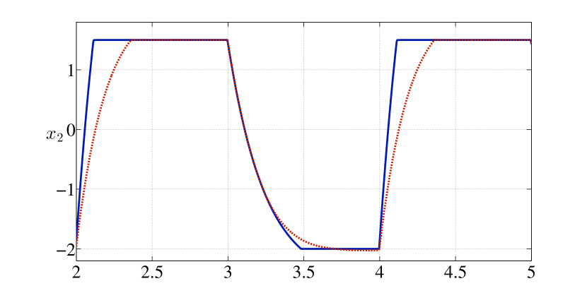
Refer to caption
Refer to caption
Refer to caption

Time (s)

Figure 1: Angular speed against time for increasing sampling periods ΔtΔ𝑡{\Delta}t and a fixed computational power 2103prox/sec2superscript103proxsec2\cdot 10^{3}~{}\nicefrac{{\text{prox}}}{{\text{sec}}}: 0.0040.0040.004 sec (top), 0.0180.0180.018 sec (middle) and 0.040.040.04 sec (bottom). The sub-optimal trajectory obtained with Algorithm 1 is plotted in dashed red, while the full NMPC trajectory obtained using ipopt (for the same ΔtΔ𝑡{\Delta}t) is in blue.
Refer to caption
Refer to caption
Refer to caption

Time (s)

Figure 2: Angular speed against time for increasing penalty parameters ρ𝜌\rho and a fixed computation power 2103prox/sec2superscript103proxsec2\cdot 10^{3}~{}\nicefrac{{\text{prox}}}{{\text{sec}}}: 202020 (top), 100100100 (middle) and 100010001000 (bottom). The sub-optimal trajectory obtained with Algorithm 1 is plotted in dashed red, while the full NMPC trajectory obtained using ipopt (for the same ΔtΔ𝑡{\Delta}t) is in blue.

In general, the computational power of an embedded computing platform is quite limited, meaning that the total number of proximal steps that can be computed within one second by Algorithms 1 and 3 is fixed and finite. Later on, we refer to this number as the computational power, expressed in prox/secproxsec\nicefrac{{\text{prox}}}{{\text{sec}}}. The results plotted in Figs. 1, 23 and 4 are obtained for a computational power of 2103prox/sec2superscript103proxsec2\cdot 10^{3}~{}\nicefrac{{\text{prox}}}{{\text{sec}}}. In Fig. 1, it clearly appears that a better tracking performance is obtained for Δt=0.018Δ𝑡0.018{\Delta}t=0.018 sec, compared to a lower sampling period (Δt=0.004Δ𝑡0.004{\Delta}t=0.004 sec) or a larger sampling period (Δt=0.04Δ𝑡0.04{\Delta}t=0.04 sec). The effect of the system’s step-size ΔtΔ𝑡{\Delta}t on the performance of Algorithm 1 given a fixed computational power is demonstrated more clearly in Fig. 5.

Another key parameter is the penalty coefficient ρ𝜌\rho, which can also be interpreted as a step-size for the optimiser. In order to demonstrate the effect of ρ𝜌\rho on the efficacy of our optimality tracking splitting scheme, the sampling period ΔtΔ𝑡{\Delta}t is fixed at 0.0180.0180.018 sec given a computational power of 2103prox/sec2superscript103proxsec2\cdot 10^{3}~{}\nicefrac{{\text{prox}}}{{\text{sec}}}, which implies that the total number of primal iterations is M=36𝑀36M=36, and ρ𝜌\rho is made vary within {20,100,1103}201001superscript103\left\{20,100,1\cdot 10^{3}\right\}. Figure 2 shows that a better tracking performance is obtained with ρ=100𝜌100\rho=100 than with ρ=20𝜌20\rho=20 or ρ=1103𝜌1superscript103\rho=1\cdot 10^{3}. This can be deduced from the expression of the coefficient βw(ρ,M)subscript𝛽𝑤𝜌𝑀\beta_{w}\left(\rho,M\right) in Eq. (4), as explained in Paragraph V-C. The optimal choice of the penalty parameter is known to be critical to the convergence speed of ADMM, which is very similar to our optimality tracking splitting scheme, since it can be interpreted as a truncated Gauss-Seidel procedure in an augmented Lagrangian. To our knowledge, this effect has only been observed for ADMM-type techniques when dealing with convex programs. When solving non-convex programs using augmented Lagrangian techniques, it is commonly admitted that ρ𝜌\rho should be chosen large enough in order to ensure (locally) positive definiteness of the hessian of the augmented Lagrangian. Taking ρ𝜌\rho too large is known to result in ill-conditioning. For Algorithm 1, which is essentially a first-order method, the analysis is different, as ρ𝜌\rho does not affect the algorithm at the level of linear algebra, but does impact the contraction of the primal-dual sequence, and thus the convergence speed over time, or tracking performance. Thus our study provides a novel interpretation of the choice of ρ𝜌\rho via a parametric analysis in a non-convex framework. The effect of the optimiser step-size ρ𝜌\rho on the closed-loop performance fully appears in Fig. 6.
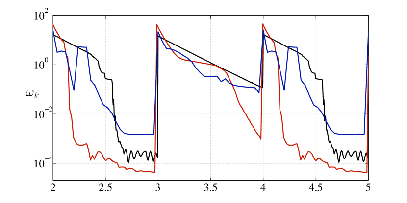
Refer to caption

Time (s)

Figure 3: Optimality of bound constrained augmented Lagrangian program for different sampling periods ΔtΔ𝑡{\Delta}t and a fixed computation power 2103prox/sec2superscript103proxsec2\cdot 10^{3}~{}\nicefrac{{\text{prox}}}{{\text{sec}}}: 0.0040.0040.004 sec (black), 0.0180.0180.018 sec (red) and 0.040.040.04 sec (blue).

Satisfaction of the KKT conditions of the parametric augmented Lagrangian problem

minimisezB(z¯,z¯)Lρ(z,μ¯k,sk+1)subscriptminimise𝑧𝐵¯𝑧¯𝑧subscript𝐿𝜌𝑧subscript¯𝜇𝑘subscript𝑠𝑘1\displaystyle\operatorname*{minimise}_{z\in B\left(\underline{z},\overline{z}\right)}~{}L_{\rho}\left(z,\bar{\mu}_{k},s_{k+1}\right)

is measured along the closed-loop trajectory by computing

ωk:=πB(z¯,z¯)(z¯(μ¯k1,sk)Lρ(z¯(μ¯k1,sk),μ¯k1,sk))\displaystyle\omega_{k}:=\|\pi_{B\left(\underline{z},\overline{z}\right)}\left(\bar{z}\left(\bar{\mu}_{k-1},s_{k}\right)-{\nabla}L_{\rho}\left(\bar{z}\left(\bar{\mu}_{k-1},s_{k}\right),\bar{\mu}_{k-1},s_{k}\right)\right)
z¯(μ¯k1,sk)2,evaluated-at¯𝑧subscript¯𝜇𝑘1subscript𝑠𝑘2\displaystyle-\bar{z}\left(\bar{\mu}_{k-1},s_{k}\right)\|_{2},\enspace

which is plotted in Fig. 3. Over time, convergence towards low criticality values is faster for Δt=0.18Δ𝑡0.18{\Delta}t=0.18 sec, than for shorter sampling period (Δt=0.004Δ𝑡0.004{\Delta}t=0.004 sec) or larger sampling period (Δt=0.04Δ𝑡0.04{\Delta}t=0.04 sec). The same effect can be observed for the feasibility of the nonlinear equality constraints G(,sk)𝐺subscript𝑠𝑘G\left(\cdot,s_{k}\right), as pictured in Fig. 4.

Refer to caption

Time (s)

Figure 4: Norm of equality constraints G(z¯k,sk)2subscriptnorm𝐺subscript¯𝑧𝑘subscript𝑠𝑘2\left\|G\left(\bar{z}_{k},s_{k}\right)\right\|_{2} for different sampling periods ΔtΔ𝑡{\Delta}t and a fixed computation power 2103prox/sec2superscript103proxsec2\cdot 10^{3}~{}\nicefrac{{\text{prox}}}{{\text{sec}}}: 0.0040.0040.004 sec (black), 0.0180.0180.018 sec (red) and 0.040.040.04 sec (blue).

From the results presented in Figures 1, 2, 3 and 4, one may conclude that sampling faster does not necessarily result in better performance of Algorithm 1. This behaviour is confirmed by Figure 5. For every computational power within {1103,2103,3103,4103}1superscript1032superscript1033superscript1034superscript103\left\{1\cdot 10^{3},2\cdot 10^{3},3\cdot 10^{3},4\cdot 10^{3}\right\}, the sampling period is made vary from Δt=2103Δ𝑡2superscript103{\Delta}t=2\cdot 10^{-3} sec to Δt=4102Δ𝑡4superscript102{\Delta}t=4\cdot 10^{-2} sec. The tracking performance is assessed by computed the normalised L2superscript𝐿2L^{2}-norm of the difference between the full-NMPC output trajectory obtained with ipopt [33] and the output signal obtained with Algorithm 1 (at the same sampling period), on a fixed time interval between 222 sec and 444 sec. More precisely, the optimality tracking error is defined by

E:=1Nsk=1Ns(yky¯k)2,assign𝐸1subscript𝑁𝑠superscriptsubscript𝑘1subscript𝑁𝑠superscriptsubscriptsuperscript𝑦𝑘subscript¯𝑦𝑘2\displaystyle E:=\sqrt{\frac{1}{N_{s}}\sum_{k=1}^{N_{s}}\left(y^{\ast}_{k}-\bar{y}_{k}\right)^{2}}\enspace,

where {yk}subscriptsuperscript𝑦𝑘\left\{y^{\ast}_{k}\right\} is the system output signal obtained with ipopt, {y¯k}subscript¯𝑦𝑘\left\{\bar{y}_{k}\right\} is the system output signal obtained with Algorithm 1 (for the same ΔtΔ𝑡{\Delta}t) and Nssubscript𝑁𝑠N_{s} is the number of time samples. For a fast sampling, the error E𝐸E appears to be quite large (11001superscript1001\cdot 10^{0}), as the warm-starting point is close to the optimal solution but only few primal proxes can be evaluated, resulting in little improvement of the initial guess in terms of optimality. This effect can even be justified further by Theorem 4: as the number of primal iterations M𝑀M is fixed by the sampling period, the term Mψ(dL,nz)superscript𝑀𝜓subscript𝑑𝐿subscript𝑛𝑧M^{-\psi\left(d_{L},n_{z}\right)} in the expression of βw(ρ,M)subscript𝛽𝑤𝜌𝑀\beta_{w}\left(\rho,M\right) and βs(ρ,M)subscript𝛽𝑠𝜌𝑀\beta_{s}\left(\rho,M\right) is not small enough to dampen the effect of the term 1+ρλG1𝜌subscript𝜆𝐺1+\rho\lambda_{G}, and thus the contraction (38) becomes looser, thus degrading the closed-loop performance. As the sampling becomes slower, more primal proximal iterations can be carried out and subsequently, the error E𝐸E is reduced. The same reasoning as before on βw(ρ,M)subscript𝛽𝑤𝜌𝑀\beta_{w}\left(\rho,M\right) and βs(ρ,M)subscript𝛽𝑠𝜌𝑀\beta_{s}\left(\rho,M\right) can be made. However, if the sampling frequency 1/Δt1Δ𝑡\nicefrac{{1}}{{{\Delta}t}} is too low, the initial guess is very far from the optimal point, to the point that Assumption 4 may not be satisfied anymore, hence the error increases again. Thus, at every computational power, an optimal sampling period is obtained. As the computation power increases, the optimal ΔtΔ𝑡{\Delta}t appears to decrease and the associated optimality tracking error E𝐸E drops.

Remark 16.

Note that we compare the behaviour of our parametric optimisation algorithm on NLPs of fixed dimension, no matter what the sampling period is, as the number of prediction samples has been fixed. This means that the prediction time changes as the sampling period varies, which may have an effect on the closed-loop behaviour. However, it is important to remember that the error E𝐸E is measured with respect to the closed-loop trajectory under the optimal full-NMPC control law computed at the same sampling period.
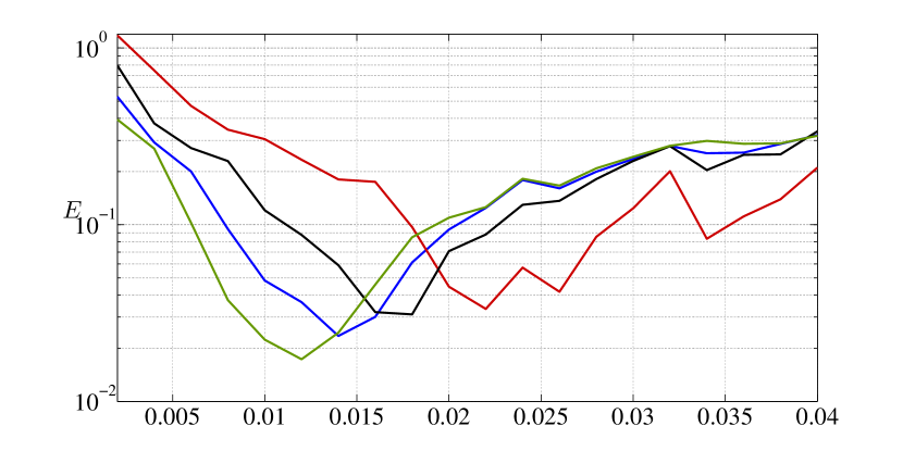
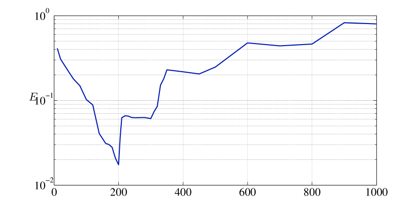
Refer to caption

Sampling period ΔtΔ𝑡{\Delta}t (s)

Figure 5: Evolution of the optimality tracking error E𝐸E against sampling period for different computation power: 11031superscript1031{\cdot}10^{3} primal iterations per sec.(red), 21032superscript1032{\cdot}10^{3} (black), 31033superscript1033{\cdot}10^{3} (blue) and 41034superscript1034{\cdot}10^{3} (green).
Refer to caption

Penalty parameter ρ𝜌\rho

Figure 6: Evolution of the optimality tracking error E𝐸E against penalty parameter ρ𝜌\rho for 2103prox/sec2superscript103proxsec2\cdot 10^{3}~{}\nicefrac{{\text{prox}}}{{\text{sec}}} and Δt=0.018Δ𝑡0.018{\Delta}t=0.018 sec.

An interesting aspect of the non-convex splitting Algorithm 1 is that the step-size ρ𝜌\rho has an effect on the closed-loop behaviour of the nonlinear dynamics, as shown in Fig. 6. Given fixed sampling period and computational power, the tracking performance can be improved by tuning the optimiser step-size ρ𝜌\rho. In a sense, ρ𝜌\rho can now be interpreted as a tuning parameter for the NMPC controller. In particular, for a fixed number of primal iterations M𝑀M, choosing ρ𝜌\rho too large makes the numerical value of the contraction coefficients βw(ρ,M)subscript𝛽𝑤𝜌𝑀\beta_{w}\left(\rho,M\right) and βs(ρ,M)subscript𝛽𝑠𝜌𝑀\beta_{s}\left(\rho,M\right) blow up, subsequently degrading the tracking performance.
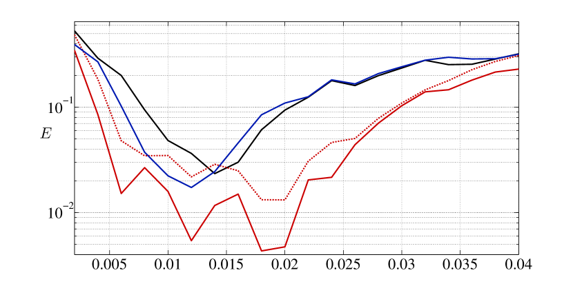
Refer to caption

Sampling period ΔtΔ𝑡{\Delta}t (s)

Figure 7: Evolution of the optimality tracking error E𝐸E against sampling period ΔtΔ𝑡{\Delta}t. Algorithm 1 for 3103prox/sec3superscript103proxsec3\cdot 10^{3}~{}\nicefrac{{\text{prox}}}{{\text{sec}}} in black, for 4103prox/sec4superscript103proxsec4\cdot 10^{3}~{}\nicefrac{{\text{prox}}}{{\text{sec}}} in blue. Algorithm 3 with 333 homotopy steps for 3103prox/sec3superscript103proxsec3\cdot 10^{3}~{}\nicefrac{{\text{prox}}}{{\text{sec}}} in dashed red, with 444 homotopy steps for 4103prox/sec4superscript103proxsec4\cdot 10^{3}~{}\nicefrac{{\text{prox}}}{{\text{sec}}} in red.

From the arguments developed in paragraph V-D of Section V, one can expect Algorithm 3 to track the time-dependent optima more closely than Algorithm 1. This is confirmed by Fig. 7.

VII-B Collaborative tracking of unicycles

The second example is a collaborative tracking problem based on NMPC. Three unicycles are controlled so that a leader follows a predefined path, while two followers maintain a fixed formation. This control objective can be translated into the cost function of an NMPC problem, which is then written

0Tx(1)(t)xr(t)Q12superscriptsubscript0𝑇superscriptsubscriptnormsuperscript𝑥1𝑡superscript𝑥𝑟𝑡subscript𝑄12\displaystyle\int_{0}^{T}\left\|x^{(1)}\left(t\right)-x^{r}\left(t\right)\right\|_{Q_{1}}^{2} +u(1)(t)R12+u(2)(t)R22superscriptsubscriptnormsuperscript𝑢1𝑡subscript𝑅12superscriptsubscriptnormsuperscript𝑢2𝑡subscript𝑅22\displaystyle+\left\|u^{(1)}\left(t\right)\right\|_{R_{1}}^{2}+\left\|u^{(2)}\left(t\right)\right\|_{R_{2}}^{2}
+u(3)(t)R32superscriptsubscriptnormsuperscript𝑢3𝑡subscript𝑅32\displaystyle+\left\|u^{(3)}\left(t\right)\right\|_{R_{3}}^{2}
+x(1)(t)x(2)(t)d1,2Q1,22superscriptsubscriptnormsuperscript𝑥1𝑡superscript𝑥2𝑡subscript𝑑12subscript𝑄122\displaystyle+\left\|x^{(1)}\left(t\right)-x^{(2)}\left(t\right)-d_{1,2}\right\|_{Q_{1,2}}^{2}
+x(1)(t)x(3)(t)d1,3Q1,32dt,superscriptsubscriptnormsuperscript𝑥1𝑡superscript𝑥3𝑡subscript𝑑13subscript𝑄132d𝑡\displaystyle+\left\|x^{(1)}\left(t\right)-x^{(3)}\left(t\right)-d_{1,3}\right\|_{Q_{1,3}}^{2}\mathrm{d}t,

where Q1,Q1,2,Q1,3,R1,R2,R3subscript𝑄1subscript𝑄12subscript𝑄13subscript𝑅1subscript𝑅2subscript𝑅3Q_{1},Q_{1,2},Q_{1,3},R_{1},R_{2},R_{3} are positive definite matrices, d1,2,d1,3subscript𝑑12subscript𝑑13d_{1,2},d_{1,3} are vectors that define the formation between unicycles 111, 222 and 333 and xr()superscript𝑥𝑟x^{r}\left(\cdot\right) is a reference path. All agents 111, 222 and 333 follow the standard unicycle dynamics

{x˙1=u1cosx3x˙2=u1sinx3x˙3=u2,\displaystyle\left\{\begin{aligned} \dot{x}_{1}&=u_{1}\cos{x_{3}}\\ \dot{x}_{2}&=u_{1}\sin{x_{3}}\\ \dot{x}_{3}&=u_{2}\end{aligned}\right.\enspace,

subject to input constraints

u1[0,0.5],u2[π2,π2].formulae-sequencesubscript𝑢100.5subscript𝑢2𝜋2𝜋2\displaystyle u_{1}\in\left[0,0.5\right]\enspace,~{}~{}~{}u_{2}\in\left[-\displaystyle\frac{\pi}{2},\displaystyle\frac{\pi}{2}\right]\enspace.
Refer to caption
Figure 8: Trajectories of the three-unicycles formation for 300prox/sec300proxsec300~{}\nicefrac{{\text{prox}}}{{\text{sec}}}, Δt=0.35Δ𝑡0.35{\Delta}t=0.35 sec and ρ=2103𝜌2superscript103\rho=2\cdot 10^{3}.

The continuous-time NMPC problem is discretised using a Runge-Kutta integrator of order 444 [20], while the closed-loop system is simulated with the matlab varying step-size integrator ode45. In the resulting finite-dimensional NLP, two cost coupling terms appear between agents 111 and 222, and agents 111 an 333. This can be addressed by the splitting Algorithm 1. Moreover, the whole procedure then consists in a sequence of proximal alternating steps between agent 111 and the group {2,3}23\left\{2,3\right\}, which can compute their proximal descents in parallel without requiring any communication. For this particular NLP with cost-couplings, the dual updates can be performed in parallel.
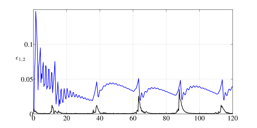
Refer to caption

Time (s)

Figure 9: Evolution of the formation error between unicycles 111 and 222 for Algorithm 1 (blue), compared with the formation error obtained with the full NMPC (ipopt, black).

Results of the collaborative tracking NMPC are presented in Figures 8 and 9. The number of iterations/communications per second has been fixed at 300300300 and the sampling period set to Δt=0.35Δ𝑡0.35{\Delta}t=0.35 sec. Within the sampling period, this results in M=105𝑀105M=105 exchanges of packets between agent 111 and agents 222,333, which perform their computations in parallel. The penalty parameter was ρ=2103𝜌2superscript103\rho=2\cdot 10^{3}. The formation-keeping NMPC has been first simulated with the unicycles in closed-loop with the full-NMPC control law, computed using ipopt with accuracy 11071superscript1071\cdot 10^{-7}, which is purely centralised, hence not very interesting from a practical point of view, in this particular case. The full-NMPC trajectory is plotted in black in Fig. 8, while the one obtained using Algorithm 1 is represented in blue. The closed-loop formation error

ϵ1,2:=x(1)x(2)d1,22assignsubscriptitalic-ϵ12subscriptnormsuperscript𝑥1superscript𝑥2subscript𝑑122\displaystyle\epsilon_{1,2}:=\left\|x^{(1)}-x^{(2)}-d_{1,2}\right\|_{2}

is plotted in Fig. 9. At every reference change, the error rises, but decreases again as the tracking converges. The performance could be further improved by tuning the penalty ρ𝜌\rho or performing a few homotopy steps as in Algorithm 3.

VIII Conclusion

An novel non-convex splitting Algorithm for solving NMPC programs in a real-time framework has been presented. Contraction of the primal-dual sequence has been proven using regularity of generalised equations and recent results on non-convex descent methods. It has been shown that the proposed Algorithm can be further improved by applying a continuation technique. Finally, the proposed approach has been analysed in details on two numerical examples.

References

  • [1] M. Alamir. Monitoring control updating period in fast gradient based NMPC. In Proceedings of the European Control Conference, pages 362136213621362636263626, July 201320132013.
  • [2] M. Alamir. Fast NMPC: a reality steered paradigm, key properties of fast NMPC algorithms. In Proceedings of the European Control Conference, 201420142014.
  • [3] E.L. Allgower and K. Georg. Introduction to numerical continuation methods. SIAM, 199019901990.
  • [4] H. Attouch and J. Bolte. On the convergence of the proximal algorithm for nonsmooth functions involving analytic features. Mathematical Programming, 116116116:555161616, 200920092009.
  • [5] H. Attouch, J. Bolte, P. Redont, and A. Soubeyran. Proximal alternating minimisation and projection methods for non-convex problems: an approach based on the Kurdyka-Lojasiewicz inequality. Mathematics of Operations Research, 353535:438438438457457457, 201020102010.
  • [6] H. Attouch, J. Bolte, and B.F. Svaiter. Convergence of descent methods for semi-algebraic and tame problems: proximal algorithms, forward-backward splitting and regularised Gauss-Seidel methods. Mathematical Programming, 137137137:919191129129129, 201320132013.
  • [7] D.P. Bertsekas. Constrained optimization and Lagrange multiplier methods. Athena Scientific, 198219821982.
  • [8] D.P. Bertsekas and J.N. Tsitsiklis. Parallel and distributed computation: numerical methods. Athena Scientific, 199719971997.
  • [9] J. Bolte, A. Daniilidis, and A. Lewis. The Lojasiewicz inequality for nonsmooth sub-analytic functions with applications to subgradient dynamical systems. SIAM Journal on Optimization, 171717:120512051205122312231223, 200720072007.
  • [10] S. Boyd, N. Parikh, E. Chu, B. Peleato, and J. Eckstein. Distributed optimization and statistical learning via the alternating direction method of multipliers. Foundations and Trends in Maching Learning, 333(111):111122122122, 201020102010.
  • [11] A.R. Conn, N.I.M Gould, and P.L. Toint. Testing a class of methods for solving minimisation problems with simple bounds on the variables. Mathematics of Computation, 505050(182182182):399399399430430430, 198819881988.
  • [12] A.R. Conn, N.I.M. Gould, and P.L. Toint. A globally convergent augmented Lagrangian algorithm for optimization with general constraints and simple bounds. SIAM Journal on Numerical Analysis, 282828:545545545572572572, 199119911991.
  • [13] D. D’Acunto and K. Kurdyka. Effective Lojasiewicz gradient inequality for polynomials. Annales Polonici Mathematici, 878787, 200520052005.
  • [14] S. Daniel-Berhe and H. Unbehauen. Experimental physical parameter estimation of a thyristor driven DC-motor using the HMF-method. Control Engineering Practice, 666:615615615626626626, 199819981998.
  • [15] M. Diehl, H.G. Bock, and J.P. Schloeder. A real-time iteration scheme for nonlinear optimization in optimal feedback control. SIAM Journal on Control and Optimization, 434343(555):171417141714173617361736, 200520052005.
  • [16] Q. Tran Dinh, I. Necoara, and M. Diehl. A dual decomposition algorithm for separable nonconvex optimization using the penalty framework. In Proceedings of the 52ndsuperscript52nd52^{\text{nd}} Conference on Decision and Control, 201320132013.
  • [17] A.L. Dontchev and R.T. Rockafellar. Characterizations of strong regularity for variational inequalities over polyhedral convex sets. SIAM Journal on Optimization, 666(444):108710871087110511051105, 199619961996.
  • [18] W.B. Dunbar. Distributed receding horizon control of dynamically coupled nonlinear systems. IEEE Transactions on Automatic Control, 525252(777):124912491249126312631263, 200720072007.
  • [19] H.J. Ferreau, H.G. Bock, and M. Diehl. An online active set strategy to overcome the limitations of explicit MPC. International Journal of Robust and Nonlinear Control, 181818:816816816830830830, 200820082008.
  • [20] E. Hairer and G. Wanner. Solving ordinary differential equations I. Springer, 200820082008.
  • [21] A. Hamdi and S.K. Mishra. Decomposition methods based on augmented Lagrangian: a survey. In Topics in nonconvex optimization. Mishra, S.K., 201120112011.
  • [22] J.-H. Hours and C.N. Jones. An augmented Lagrangian coordination-decomposition algorithm for solving distributed non-convex programs. In Proceedings of the American Control Conference, 201420142014.
  • [23] F. Lin, M. Fardad, and M.R. Jovanovic. Design of optimal sparse feedback gains via the alternating direction method of multiplers. IEEE Transactions on Automatic Control, 585858(999), 201320132013.
  • [24] I. Necoara, C. Savorgnan, Q. Tran Dinh, J. Suykens, and M. Diehl. Distributed nonlinear optimal control using sequential convex programming and smoothing techniques. In Proceedings of the 48thsuperscript48th48^{\text{th}} Conference on Decision and Control, 200920092009.
  • [25] Y. Nesterov. Efficiency of coordinate descent methods on huge-scale optimization problems. SIAM Journal on Optimization, 222222(222):341341341362362362, 201220122012.
  • [26] M.J.D. Powell. On search directions for minimisation algorithms. Mathematical Programming, 444:193193193201201201, 197319731973.
  • [27] Stephen M. Robinson. Strongly regular generalised equations. Mathematics of Operations Research, 555(111):434343626262, 198019801980.
  • [28] R.T. Rockafellar. Augmented Lagrangian multiplier functions and duality in non-convex programming. SIAM Journal on Control and Optimization, 121212(222):268268268285285285, 197419741974.
  • [29] R.T. Rockafellar and R. J.-B. Wets. Variational Analysis. Springer, 200920092009.
  • [30] B.T. Stewart, S.J. Wright, and J.B. Rawlings. Cooperative distributed model predictive control for nonlinear systems. Journal of Process Control, 212121(555):698698698704704704, 201120112011.
  • [31] Q. Tran Dinh, C. Savorgnan, and M. Diehl. Adjoint-based predictor-corrector sequential convex programming for parametric nonlinear optimization. SIAM Journal on Optimization, 222222(444):125812581258128412841284, 201220122012.
  • [32] P. Tseng. Convergence of a block coordinate descent method for nondifferentiable minimization. Journal of Optimization Theory and Applications, 109109109(333):475475475494494494, 200120012001.
  • [33] A. Waechter and L.T. Biegler. On the implementation of a primal-dual interior point filter line-search algorithm for large-scale nonlinear programming. Mathematical Programming, 106106106(111):252525575757, 200620062006.
  • [34] V.M. Zavala and M. Anitescu. Real-time nonlinear optimization as a generalised equation. SIAM Journal on Control and Optimization, 484848(888):544454445444546754675467, 201020102010.
  • [35] V.M. Zavala and M. Anitescu. Scalable nonlinear programming via exact differentiable penalty functions and trust-region Newton methods. SIAM Journal on Optimization, 242424(111):528528528558558558, 201420142014.
  • [36] V.M. Zavala and L.T. Biegler. The advanced-step NMPC controller: optimality, stability and robustness. Automatica, 454545(111):868686939393, 200920092009.