Ensemble Kalman filter data assimilation in a Babcock-Leighton solar dynamo model: an observation system simulation experiment for reconstructing meridional flow-speed

Abstract

Accurate knowledge of time-variation in meridional flow-speed and profile is crucial for estimating a solar cycle’s features, which are ultimately responsible for causing space climate variations. However, no consensus has been reached yet about the Sun’s meridional circulation pattern observations and theories. By implementing an Ensemble Kalman Filter (EnKF) data assimilation in a Babcock-Leighton solar dynamo model using Data Assimilation Research Testbed (DART) framework, we find that the best reconstruction of time-variation in meridional flow-speed can be obtained when ten or more observations are used with an updating time of 15 days and a $\leq 10\%$ observational error. Increasing ensemble-size from 16 to 160 improves reconstruction. Comparison of reconstructed flow-speed with “true-state” reveals that EnKF data assimilation is very powerful for reconstructing meridional flow-speeds and suggests that it can be implemented for reconstructing spatio-temporal patterns of meridional circulation.

1 Introduction

In recent years simulations of Babcock-Leighton type flux-transport (hereafter BLFT) solar dynamos in both 2D and 3D (Wang & Sheeley, 1991; Dikpati & Charbonneau, 1999; Miesch & Dikpati, 2014) demonstrated the crucial role the Sun’s global meridional circulation plays in determining solar cycle properties. Time variations in speed and profile of meridional circulation have profound influence on solar cycle length and amplitude. The recent unusually long minimum between cycles 23 and 24 has been explained by implementing two plausible changes in meridional circulation, (i) by implementing the change from a two-celled profile in latitude in cycles 22 to a one-celled profile in cycle 23 (Dikpati et al, 2010), and (ii) by performing a vast number of simulations by introducing a flow-speed change with time during the declining phase of each cycle (Nandy, Muñoz-Jaramillo & Martens, 2011). Accurately knowing the speed and profile variations of the meridional circulation would greatly improve prediction of solar cycle features.

The meridional circulation has been observed in the photosphere and inside the upper convection zone in the latitude range from the equator to $\sim 60^{\circ}$ in each hemisphere (Ulrich, 2010; Komm et  al., 2013; Zhao et  al., 2013; Schad, Timmer & Roth, 2013; Kholikov, Serebryanskiy & Jackiewicz, 2014). However, the speed, pattern and time variations of the circulation at high latitudes and in the deeper convection zone are not known from observations yet. Theoretical models of meridional circulation (Miesch, 2005; Dikpati, 2014) provide some knowledge, but the flow patterns derived from model outputs vary from model to model, primarily because of our lack of knowledge of viscosity and density profiles and thermodynamics in the solar interior, which are essential ingredients in such models. As differential rotation does not change much with time compared to meridional circulation, in this first study we focus on time variation of meridional flow-speed, using a set-up similar to that used previously (Charbonneau & Dikpati, 2000; Nandy, Muñoz-Jaramillo & Martens, 2011). Since the meridional circulation is a specified parameter in kinematic BLFT dynamos and the dynamo solutions depend sensitively on the spatio-temporal patterns of this circulation, we ask the question: can we infer the meridional circulation (in both space and time) from observations of the magnetic field? The purpose of this paper is to describe an Ensemble Kalman Filter (EnKF) data assimilation in a 2D BLFT solar dynamo model for reconstructing meridional flow-speed as a function of time for several solar cycles. A subsequent paper will investigate the reconstruction of spatio-temporal patterns of meridional circulation in the solar convection zone.

Data assimilation approaches have been in use for several decades in atmospheric and oceanic models, but such approaches have been implemented in solar and geodynamo models only recently. Jouve, Brun & Talagrand (2011) introduced a variational data assimilation system into an $\alpha$-$\Omega$ type solar dynamo model to reconstruct the $\alpha$-effect using synthetic data. Very recently Svedin, Cuéllar & Brandenburg (2013) applied a variational data assimilation method to estimate errors of the reconstructed system states in a stratified convection model. A detailed discussion of data assimilation in the context of the geodynamo can be found in Fournier et  al. (2010).

In a sequential data assimilation framework, a set of dynamical variables at a particular time defines a ”model state”, which is the time-varying flow speed in the context of the present paper. Scalar functions of these state variables that can also be observed using certain instruments are called ”observation variables”, which are magnetic fields here. More detailed terminology for identifying data assimilation components with solar physics variables is given in §2. In brief, the goal of sequential data assimilation is to constrain the model state at each time-step to obtain model-generated observation variables that are as close to the real observations as possible. The basic framework is based on statistical multidimensional regression analysis, a well-developed method that has been applied in atmospheric and oceanic studies (see Anderson (2001); Anderson et al (2005); Anderson & Collins (2007) for details). The EnKF sequential data assimilation framework also allows adding model parameters to the set of model states and estimating values of these parameters that are most consistent with the observations.

It is a common practice to perform an “Observation System Simulation Experiment” (OSSE) in order to validate and calibrate the assimilation framework for a particular model. An OSSE generates synthetic observations from the same numerical model that is used in the assimilation. In this case the numerical model is a simple BLFT dynamo model containing only a weak nonlinearity in the $\alpha$-quenching term; thus adding Gaussian noise to model-outputs for producing synthetic observations works well. In a more realistic situation for a large system with highly nonlinear processes, such as in numerical weather prediction models, it may be necessary to use a non-Gaussian ensemble filter (see, e.g. Anderson (2010)).

A few examples of predicting model parameters using sequential data assimilation techniques have been presented by Minter, Fuller-Rowell & Codrescu (2004) and Codrescu, Minter & Fuller-Rowell (2004) in the context of estimating neutral thermospheric composition, and most recently by Matsuo, Lee & Anderson (2013) for estimating thermospheric mass density. An EnKF data assimilation framework has recently been applied to a 3D, convection-driven geodynamo model for full state estimation using surface poloidal magnetic fields as observations (Fournier, Nerger & Aubert, 2013). We implement EnKF sequential data assimilation to reconstruct time-variations in meridional flow-speed for several solar cycles, using poloidal and toroidal magnetic fields as observations. We note certain differences in our case compared to the cases described above, namely, unlike neutral thermospheric composition and thermospheric mass density, the meridional flow-speed is not governed by a deterministic equation.

2 Methodology and Assimilation setup

In order to describe the EnKF data assimilation methodology, we first identify the data assimilation components with solar physics variables. A physical BLFT dynamo model, which generates magnetic field data for a given the meridional flow-speed, is called the “Forward Operator”. The time-varying meridional flow-speed at a given time is the “model state” and will be estimated by the EnKF system. The EnKF requires a prediction model that generates a forecast of the meridional flow-speed at a later time given the value at the current time. Here, that prediction model simply adds a random draw from a Gaussian distribution to the current meridional flow-speed, because the BLFT dynamo model we are using here is a kinematic dynamo model. In the future, the results can be further refined by imposing additional physical conditions using a dynamical dynamo model. It is important not to confuse the prediction model with the BLFT dynamo model that acts as a forward operator for the data assimilation process.

Figure 1 schematically depicts the data assimilation framework considering an “ensemble of three members” of the prediction model state (meridional flow-speeds). Sequential assimilation can usually be described as a two-step procedure, a forecast followed by an analysis each time an observation is available. In Figure 1, ${v_{1}}^{t},{v_{2}}^{t},{v_{3}}^{t}$ near the label (a) denote three different realizations of initial flow-speeds, which are input to the prediction model. We generate “prior” estimates of the model state (denoted by ${v_{1}}^{{t+\delta}^{\rm\,prior}},{v_{2}}^{{t+\delta}^{\rm\,prior}},{v_{3}}^{{t+\delta}^{\rm\,prior}}$ near the label (b)) by using the prediction model to advance the estimates of the flow-speed from the initial time ($t$) to the time ($t+\delta$) at which the first observations of magnetic field are available. In this case, the prediction model just adds a different draw from the Gaussian noise distribution to each initial ensemble estimate of the flow speed ($\Gamma$ along the solid green arrows in Figure 1). The resulting ensemble of flow speeds is referred to as a prior ensemble estimate. The central equation for estimating the prior state is a stochastic equation given by,

$${v_{1}}^{{t+\delta}^{\rm prior}}={v_{1}}^{t}+\Gamma_{0}\times\gamma,\quad$$

in which, $\gamma$ is a function for generating normalized Gaussian random numbers with unit amplitude and unit standard deviation, and the amplitude of the prediction model noise is governed by $\Gamma_{0}$. Thus the evolution of the system from label (a) to (b) through Equation (1), denoted by ’Eq1’ in Figure 1, constitutes the first step of the two-step procedure in sequential assimilation.

Figure 1: Schematic representation of the EnKF method as applied in present problem. Three members of the ensemble of flow-speeds at time $t$, namely $V_{1}^{t}$, $V_{2}^{t}$ and $V_{3}^{t}$ are evolved using Equation (1) to generate corresponding prior state at time $t+\delta$, shown as evolution from (a) to (b). In the “Filter” box, observations $O_{1}$, $O_{2}$ and $O_{3}$ are generated by applying forward operator (FTD) on the prior estimates. Then following a linear regression analysis on these observations with corresponding flow-speeds, the “Filter” estimates posterior flow-speeds using the synthetic observation with errors. In the process it also generates the posterior observation for evaluation of innovation at time $t+\delta$. Time advances from $t$ to $t+\delta$ (denoted by solid line at the top) during the evolution from (a) to (b), while in the “Filter” procedure, time remains frozen at step $t+\delta$ (denoted by dotted line from (b) to (c)).

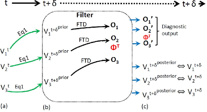
The second step includes (i) producing observations from outputs of the forward operator and (ii) estimating posterior flow-speeds by employing regression among these observations, real observations (synthetic in OSSE) and prior flow-speeds. The forward operator (BLFT dynamo in this case) is denoted by ${\rm FTD}$ along the solid black arrows, which uses the prior estimates of flow speed to produce a prior “ensemble of observation estimates” which are magnetic field outputs. Three realizations of magnetic fields from the forward operator are denoted by $O_{1}$, $O_{2}$, $O_{3}$ in Figure 1. Note that the statement, “forward operator operating on three model states generates three prior observation estimates”, is equivalent to the statement, “BLFT dynamo running with three meridional flow speeds produces three sets of model outputs of magnetic fields”.

To elucidate the second step of assimilation, we describe the function of the “Filter”. For real prediction using EnKF data assimilation, we would have real data (observations) from instruments; in our OSSE case it is synthetic, denoted by $\Phi^{T}$ in Figure 1. Synthetic observations are generated by applying the forward operator to a specified time series of meridional flow-speeds (as shown in Figure 2a). Our goal is to apply an EnKF to obtain an improved distribution of estimated flow-speeds (i.e. “posterior states”, ${v_{1}}^{{t+\delta}^{\rm\,posterior}},{v_{2}}^{{t+\delta}^{\rm\,posterior}},{v_{3}}^{{t+\delta}^{\rm\,posterior}}$) using the prior ensemble and the observation of magnetic field. The EnKF (black-dotted box in the diagram) first compares the prior ensemble of observation-estimates to the actual observation and computes increments to the prior observation-estimates. These observation-increments are then regressed using the joint prior-ensemble distribution of flow-speed and magnetic field observations to compute increments for the prior-ensemble of flow-speeds. The EnKF can also produce a posterior-ensemble of magnetic field observations (${O_{1}}^{\prime},{O_{2}}^{\prime},{O_{3}}^{\prime}$), which can be used for diagnostic purposes. The posterior-ensemble distribution of flow-speeds is the best estimate of the flow-speed distribution at time $t+\delta$ given the available observations. Mean flow-speed at time $t+\delta$ can be calculated by taking the average over all ensemble members.

To proceed with the reconstruction of flow-speeds at the time of the next observation, $t+2\delta$, the reconstructed flow-speeds at time $t+\delta$ are used as the input to the prediction model (Equation (1)), and the same procedure described in the previous paragraphs is repeated. Random Gaussian noise through Equation (1) prevents degeneration of ensemble. Thus after many time steps, the entire time series of the ensemble distribution of flow-speeds can be constructed. Time series of the mean flow-speeds can be calculated by taking the average over all ensemble members at each time. However, it may produce a better reconstruction in some cases if one ensemble member, which produced observation ($O^{\prime}$) closest to real observation ($\Phi^{T}$), is chosen.

In order to perform an OSSE, it is now necessary to define the “true state” flow-speed as a function of time. Synthetic observations are generated at selected times by applying the forward operator (BLFT dynamo model) to the true state flow-speed at the appropriate time and adding on a random draw from a specified observational error distribution to simulate instrumental and other errors.

Figure 2: Panel (a): true state (i.e. time-varying meridional flow speed) that varies by $\pm 70\%$ about mean flow-speed, $14\,{\rm m}{\rm s}^{-1}$; Panel (b): synthetic observations with observational error bars, shown at selected finite intervals for clarity.

As noted above, the forward operator is a kinematic BLFT dynamo model, described in detail in Dikpati et al (2010). The dynamo ingredients are a solar-like differential rotation, a single-celled meridional circulation, a Babcock-Leighton type surface $\alpha$-effect and a depth-dependent diffusivity; the mathematical forms are prescribed in Dikpati et al (2010). Dynamo equations, computation domain and boundary conditions are used as given in Dikpati et al (2010). At $t=0$ we start the integration of the dynamo-DART system over the first assimilation-step by initializing the forward operator (FTD model) with a converged solution for a flow-speed of $14\,{\rm m}{\rm s}^{-1}$. In the subsequent assimilation-steps, the solution at the end of previous assimilation-step for each ensemble-member is used as initial condition.

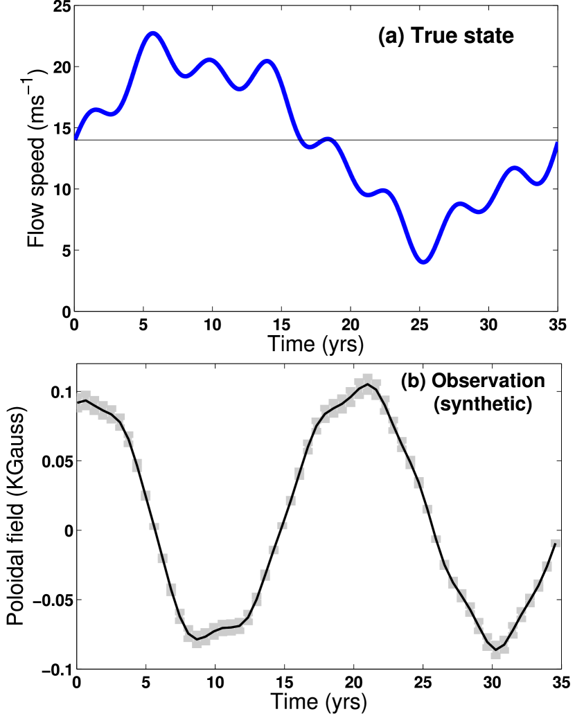
We construct a time-varying flow-speed for a span of 35 years (see Figure 2(a)), guided by observations (Basu & Antia, 2010; Ulrich, 2010), which has a natural variation of 20-40% with respect to the mean flow considered here, i.e. 14 ${\rm m}{\rm s}^{-1}$, as shown by the thin black line in Figure 2(a). This specified time-varying flow-speed is referred to as the true model state. Thus, keeping the spatial pattern of meridional circulation fixed, we consider here reconstructing the time-series of the scalar flow-speed.

To generate synthetic magnetic field data, we incorporate the time-varying true meridional flow-speed in our BLFT dynamo, and simulate the time series of idealized magnetic fields in the entire computation domain. Then we construct the time series of synthetic magnetic observations by adding synthetic observational error to the simulated idealized magnetic data. Figure 2(b) shows a single observation, which is created from the simulated poloidal field by extracting from the location, $r=0.98R$ and $\theta=86.5^{\circ}$. However, note that the dynamo simulation in $101\times 101$ grids can give us as many as 20202 synthetic magnetic observations of poloidal and toroidal fields.

3 Results

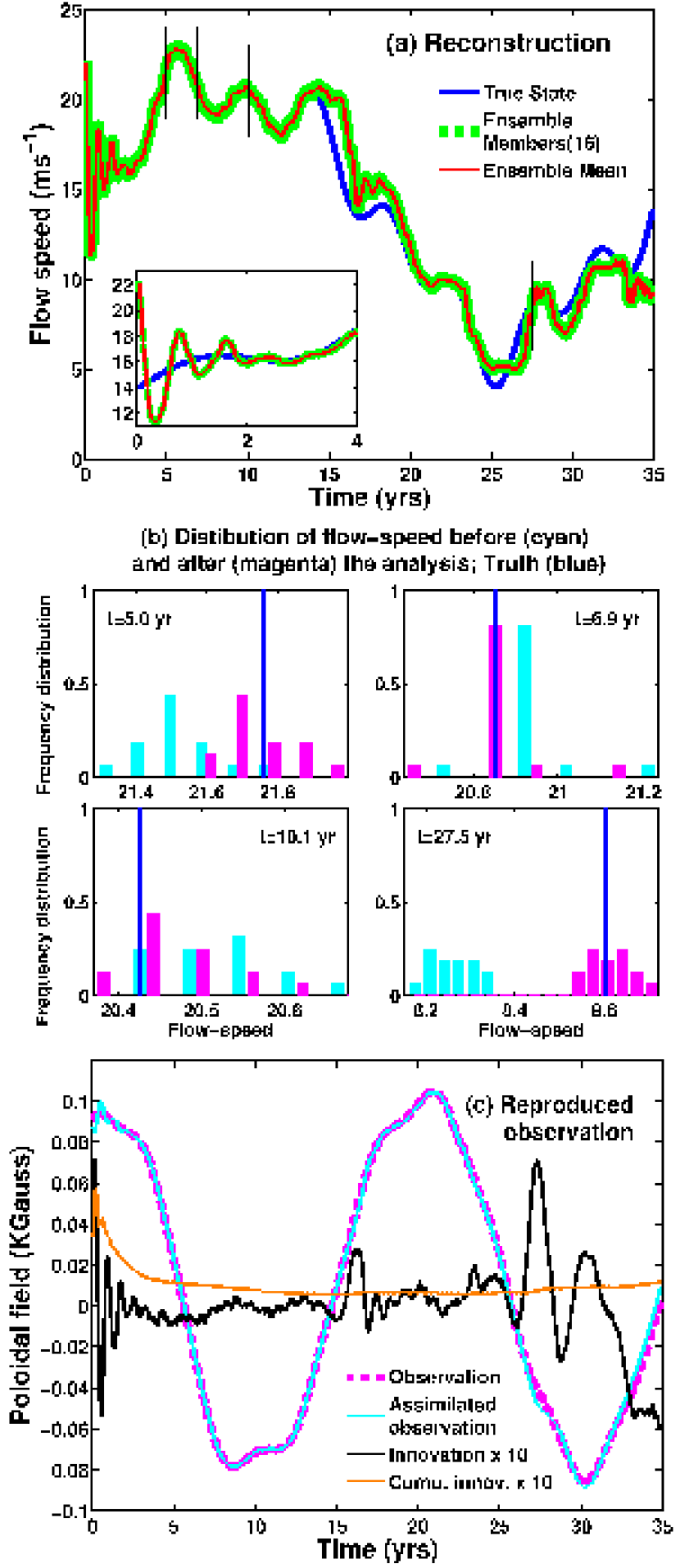
Considering only one observation, as shown in Figure 2(b), we perform assimilation runs with 16 ensemble members with an observational error of $\sim 30\%$, which means an error of $\sim 30\%$ about the ideal magnetic field generated using the true meridional flow speed. To estimate the prior states of flow-speed, we use Equation (1), in which we set $\Gamma_{0}=0.5{\rm m}{\rm s}^{-1}$. If the meridional flow-speed varies up to $\pm 20\%$ (i.e. $\sim\pm 2.8{\rm m}{\rm s}^{-1}$ for a mean flow-speed of $14{\rm m}{\rm s}^{-1}$) during six months, the variation in 15 days can be $\sim 0.23{\rm m}{\rm s}^{-1}$. Thus we chose $\Gamma_{0}=0.5{\rm m}{\rm s}^{-1}$ so that it is large enough to capture the variation in flow-speed within our selected updating time-step of 15 days and also large enough to avoid ensemble collapse, but not so large as to produce unusual departures from cyclic behavior in a flux-transport dynamo. We show in Figure 3 the reconstructed meridional flow-speed as a function of time (panel (a)) and the estimates of the observation computed from the flow speed ensemble after data assimilation (panel (b)).

We see in Figure 3(a) that the reconstruction is reasonably good except for the time windows between $\sim 15$ to 18 years and 33 to 35 years during which we find $\sim 40\%$ error in the reconstructed flow speed. Observations indicate $\sim 10-20\%$ error in the measurement of meridional flow speed (Basu & Antia, 2010; Ulrich, 2010). The inset of Figure 3(a) reveals, for an initial guess, far-off from the true-state, the reconstructed states asymptotically converges towards the true-state. Even though they oscillate around the truth with large amplitude, the oscillations damp with time. Figure 3(b) shows histograms for the normalized distribution of flow-speeds before (in cyan) and after (in magenta) the analysis stage, along with true-state (blue), for the time instances of 5, 6.9, 10.1 and 27.5 years (marked by vertical lines in Figure 3(a)) during assimilation. For this case with 16 ensemble members we chose 10 bins for an optimal display. Four time instances are chosen in such a way as to present the following four different phases of reconstructions: (i) the distribution of prior and posterior states has small overlap (top left frame of Figure 3(b)), (ii) distribution is sharply peaked in one bin each for prior and posterior (top right frame), (iii) distribution is broad and has significant overlap (bottom left frame) and (iv) distribution has no overlap at all (bottom right frame). However, we can clearly see the successful performance of the EnKF which reveals that in all cases the analysis phase brings the posterior distribution (magenta bars) closer to true-state (blue).

Figure 3(c) reveals that the assimilated magnetic observation (blue solid curve) is well-reproduced when compared with real observation (red-dashed curve). This is not surprising, because it has already been noted that short-term small fluctuations in flow speed do not significantly influence the overall evolution of global magnetic fields generated by a Babcock-Leighton dynamo (see, e.g. Belucz & Dikpati (2013)). We also plot the innovation ($I_{i}$) for this observation (black curve) and the cumulative innovation (orange curve). The innovation at the $i^{th}$ analysis-step ($I_{i}$) is defined as the signed difference between real and reconstructed observations, whereas the cumulative innovation ($CI_{i}$) at $i^{th}$ analysis-step is the normalized sum of norm of innovation vectors over all the previous analysis-steps. $I_{i}$ and $CI_{i}$ being small, both have been ten-fold magnified to superimpose on observations. We see that, at three different time instances ($t\approx 0$, 17 and 27 years), the innovation is relatively large; this is because at $t=0$ the initial guess is far-off from the truth, and at $t\approx 17$ and 27 years there are relatively sharp changes in flow-speed. The cumulative innovation asymptotes to zero as expected, implying no bias of the system. To investigate the possibility of further improvement in the quality of the EnKF reconstruction, we examine the consequences of three important aspects of the EnKF: variation in observational error, size of ensemble and number of observations.

Figure 3: In panel (a), red curve denotes ensemble-mean of reconstructed meridional flow-speeds as a function of time; superimposed green curves denote all 16 ensemble members; true state is plotted in blue for comparison. Panel (b) shows normalized distribution of flow-speed in a histogram plot for four different times. The prior, posterior and true state are plotted in cyan, magenta and blue respectively. Panel (c) shows estimated observation after assimilation (i.e. poloidal magnetic field at $r=0.98R$ and $\theta=86.5^{\circ}$) in blue and actual observation in red; superimposed on that are innovation (black) and cumulative innovation (orange) (both ten-fold magnified for clarity).

Figure 4: Panels (a, b, c) show errors in reconstruction (in units of ${\rm m}{\rm s}^{-1}$) respectively as functions of observational errors (a), size of ensemble (b) and number of observations (c).

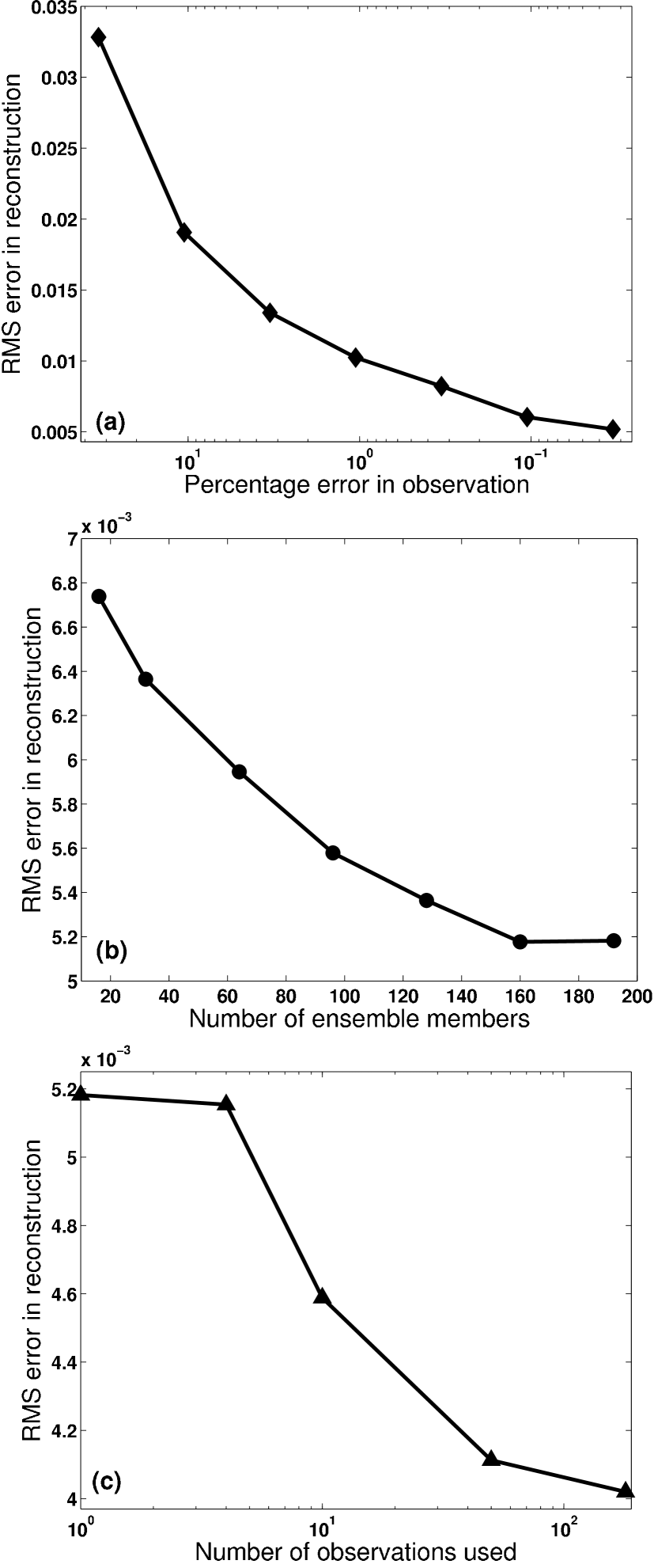
We perform convergence tests by estimating the error in the reconstructed state as functions of observational errors, size of ensemble and number of observations. We define the error as the root mean square of the difference between the reconstructed state and the true-state. The assimilation interval is chosen to be 15 days in the present case; denoting every 15 days by the index $i$, the true state and the reconstructed state at the $i^{th}$ assimilation step by ${V_{T}}^{i}$ and ${V_{R}}^{i}$ respectively, we define the error as, $\sum_{i=1}^{n_{\rm max}}\sqrt{{({V_{T}}^{i}-{V_{R}}^{i})}^{2}}/n_{\rm max}$, in which $n_{\rm max}$ is the total number of indices for the 15-days assimilation intervals during the entire time-span of 35 years.

Figure 4 shows the rms errors in reconstructed flow speed as functions of observational error (Figure 4(a)), size of ensemble (Figure 4(b)) and number of observations (Figure 4(c)). We see in Figure 4 that the error decreases systematically and asymptotes for certain values of the observational errors (1%), size of ensemble (192 members) and number of observations (180). In the case of more than one observation, we include more poloidal field observations (synthetic) from various locations at and near the surface, and more toroidal field observations at and near the bottom of the convection zone. While we vary observational errors in panel (a), we use $1\%$ observational error in panels (b) and (c). Panels (a,b) show convergence to typical hyperbolic patterns, as is often seen in numerical convergence tests (see, e.g. figure 3 of Dikpati (2012)). But panel (c) shows that the reconstruction can be improved systematically only when there are more than a certain number of observations (four in our case). In all these experiments, we used the same EnKF scheme.

Bias or systematic error in an OSSE reconstruction may arise primarily because of the following assumptions made in the assimilation system: (i) the evolution of the ensemble spread is linear, (ii) the ensemble is sufficiently large, (iii) the forward operators are linear. Though these assumptions are roughly valid, they are not strictly true. But in general, the resulting systematic errors are small unless the assimilation is applied in a large, highly nonlinear system like a numerical weather prediction model.

Figure 5: As in Figure 3(a), red and green curves denote reconstructed meridional flow-speed, 192 reconstructions for 192 ensemble members as function of time. Total 180 observations with observational error of $1\%$ have been used. Note that the true state (blue) is invisible, hidden behind the red and green curves.

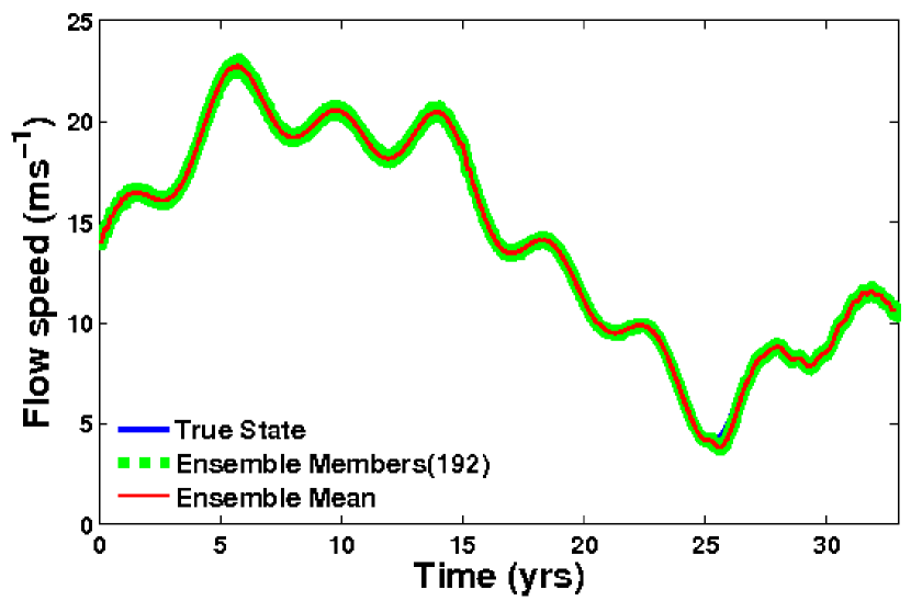
With the knowledge gained from the convergence experiments shown in Figure 4, we consider a case with 192 ensemble members and 180 magnetic observations, consisting of equal numbers of poloidal and toroidal magnetic fields at various latitude and depth locations. Each of these observations has an observational error of $1\%$. We present the reconstructed flow-speed from this assimilation in Figure 5. The reconstructed flow-speed (red curve) matches very well with the true state, and thus the true state plotted in blue is essentially hidden behind red and green curves. It is not realistic to expect an observational error of as small as 1%; Figure 5 presents here an illustrative example of one of the best possible reconstructions. In fact, several additional assimilation runs indicate that the reconstruction is still good if the observational error does not exceed 40%, and reasonably good when 90 out of 180 observations have up to $\sim 50\%$ errors. But the reconstruction fails when all observations have more than 40% error.

What we have demonstrated so far is that the time-dependent amplitude of meridional circulation, having one flow-cell per hemisphere, can be reconstructed by implementing EnKF data assimilation with synthetic data. In reality we do not know from observational data whether they were produced by a dynamo operating with a single-celled flow in each hemisphere, or with a more complex flow profile, or with a combination of complex time-variations in all possible dynamo ingredients. In order to investigate the outcome from this method when the assumption made about the flow profile is wrong, we carry out an experiment to reconstruct flow-speed assuming a one-cell flow, while using observations of magnetic fields produced from a flow pattern that has two cells in latitude in each hemisphere (see Dikpati et al (2010) for prescription of a two-celled flow). We obtain synthetic data for a case with two flow cells in latitude. Using 192 ensemble members and 180 magnetic observations with 1% error in each of these observations, we estimate the time variation in flow-speed by assuming a single-celled flow, and plot in Figure 6(a). We find that the reconstruction is relatively poor, as expected. However, with a closer look we can see that the reconstructed speed is trying to approach the true-state from a lower value for the first 12 years and from a higher value for the next 13 years. When the trend in the true-state reverses near the year 27, the OSSE has greater difficulty in converging on it.

Figure 6: (a) Same as in Figure 5, but for a case in which assumption made about spatial structure of flow is incorrect. (b) Two characteristic innovations for observations at $\theta=86.5^{\circ}$ and $3.6^{\circ}$ are plotted respectively in magenta and black curves, and cumulative innovation in orange curve.

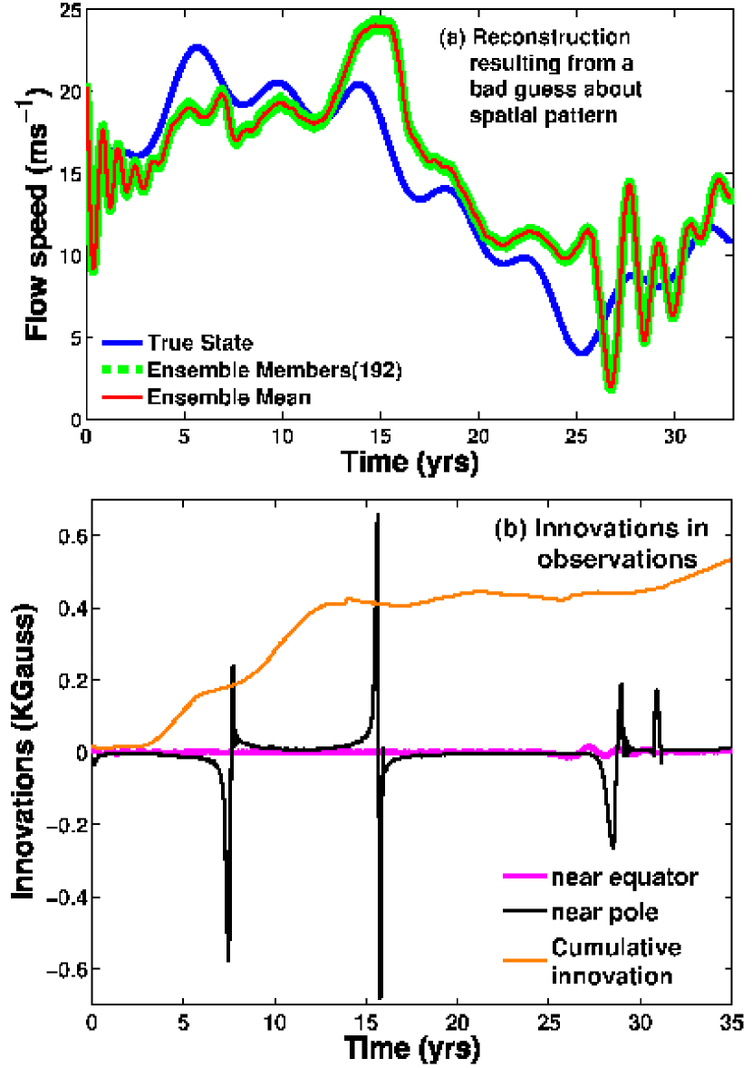
Figure 6(b) shows the innovation for two typical observations of poloidal fields near the surface, at $\theta=86.5^{\circ}$ (i.e. at low latitude near the equator) and at $3.6^{\circ}$ (at high latitude near the pole). Much larger innovation at high latitude than at low latitude reflects the fact that the spatial pattern is more erroneous at polar latitudes. The cummulative innovation (orange curve) does no longer asymptote to zero; this implies bias in the system, due to incorrect assumption of flow-pattern. In the future, we will extensively explore the reconstruction of spatial pattern of meridional circulation.

4 Comments and conclusions

We have demonstrated through OSSEs that EnKF data assimilation into a Babcock-Leighton flux-transport dynamo can successfully reconstruct time-varying meridional circulation speed for several cycles from observations of the magnetic field. To obtain the best reconstruction, we have fed the assimilation system of 192 ensemble members with 180 observations with 1% observational error. However, a reasonably good reconstruction can be obtained when all observations have up to $40\%$ error, or half of the observations have up to $50\%$ errors, but the rest of them have much smaller errors.

Dikpati & Anderson (2012) noted that the response time of a Babcock-Leighton dynamo model to changes in meridional flow is $\sim 6$ months, so the relatively poor reconstruction with only one observation with 33% observational error and 16 ensemble members can be improved if this information about the dynamo model’s response time to flow changes can be exploited. A forthcoming paper will investigate how to use this response time during assimilation.

Throughout this paper, we used an assimilation interval of 15-days. The reason for this choice is as follows. Recently Sanchez, Fournier & Auburt (2014) have done a very thorough assessment of the ’predictability’ of solar flux-transport dynamos. Predictability of a model refers to the time it takes for two solutions that start from slightly different values of either initial conditions or input parameters to diverge from each other to the point that they forecast substantially different outcomes. Sanchez, Fournier & Auburt (2014) found an $e$-folding time of about 30 years. The flux-transport dynamo model we use here is physically very similar to theirs. Therefore we judge that the $e$-folding time for our model will be similar.

It is clear that the time interval for updating the data in our OSSE’s should be much less than the predictability limit of the model, but it should be long compared to the integration time step (a few hours), and consistent with the time scale for changes in axisymmetric solar observations, which is one solar rotation. It should also be shorter than the ”response time” of our dynamo model ($\sim 6$ months, see Dikpati & Anderson (2012)) to a sudden change in inputs. We have therefore chosen our updating interval to be 15 days; we plan to test the sensitivity of assimilation to changes in the updating interval from 15 days to longer (for instance, 30 days) and shorter ($\sim 3$ days).

In this study we have demonstrated what it takes to reconstruct the amplitude variations with time of a one-celled meridional circulation of fixed profile with latitude and radius. In reality the Sun’s meridional circulation may not be a one-celled pattern – it may undergo changes both in profile and speed with time. We have demonstrated that the innovation in observation-forecast can be very large when the assumption about the spatial structure of the flow-pattern is incorrect, and it can be even larger where the departure in assumed spatial pattern from actual pattern in flow is larger. Thus an obvious next step with our data assimilation system would be to attempt to reconstruct the spatio-temporal pattern of meridional flow.

Our ultimate goal is to perform assimilation runs from actual observations instead of synthetic data, in cases of reconstruction as well as future predictions. From this study we can build confidence about the power of EnKF data assimilation for reconstructing not only the flow speed but also the profile of meridional circulation in the entire convection zone of the Sun in the future.

References

- Anderson (2001) Anderson, J. L., An ensemble adjustment Kalman filter for data assimilation, Mon. Wea. Rev., 129, 2884-2903, 2001
- Anderson et al (2005) Anderson, J. L., Wyman, B., Zhang, S. & Hoar, T., Assimilation of surface pressure observations using an ensemble filter in an idealized global atmospheric prediction system, J. Atmos. Sci., 62, 2925-2938, 2005
- Anderson & Collins (2007) Anderson, J. & Collins, N., J., Scalable Implementations of Ensemble Filter Algorithms for Data Assimilation, Journal of Atmos. and Oceanic Tech., 24, 1452-1463, 2007
- Anderson (2010) Anderson, J. L., A Non-Gaussian Ensemble Filter Update for Data Assimilation, Mon. Wea. Rev., 138, 4186-4198, 2010
- Basu & Antia (2010) Basu, S. & Antia, H. M., Characteristics of Solar Meridional Flows during Solar Cycle 23, ApJ, 717, 488-495, 2010
- Belucz & Dikpati (2013) Belucz, B. & Dikpati, M., Role of Asymmetric Meridional Circulation in Producing North-South Asymmetry in a Solar Cycle Dynamo Model, ApJ, 779, 4, 1-9, 2013
- Codrescu, Minter & Fuller-Rowell (2004) Codrescu, M. V., Minter, C. F. & Fuller-Rowell, T. J., An ensemble-type Kalman filter for neutral thermospheric composition during geomagnetic storm, Space Weather, 2, S11002, 1-9, 2004
- Charbonneau & Dikpati (2000) Charbonneau, P. & Dikpati, M., Stochastic Fluctuations in a Babcock-Leighton Model of the Solar Cycle, ApJ, 543, 1027-1043, 2000
- Dikpati & Charbonneau (1999) Dikpati, M. & Charbonneau, P., A Babcock-Leighton Flux Transport Dynamo with Solar-Like Differential Rotation, ApJ, 518, 508-520, 1999
- Dikpati et al (2010) Dikpati, M., Gilman, P. A., de Toma, G., & Ulrich, R. K., Impact of changes in the Sun’s conveyor-belt on recent solar cycles, Geophys. Res. Lett., 37, L14107, 1-6, 2010
- Dikpati & Anderson (2012) Dikpati, M. & Anderson, J. L., Evaluating Potential for Data Assimilation in a Flux-transport Dynamo Model by Assessing Sensitivity and Response to Meridional Flow Variation, ApJ, 756, 20, 1-14, 2012
- Dikpati (2012) Dikpati, M., Nonlinear Evolution of Global Hydrodynamic Shallow-water Instability in the Solar Tachocline, ApJ, 745, 128, 1-20, 2012
- Dikpati (2014) Dikpati, M., Generating the Sun’s global meridional circulation from differential rotation and turbulent Reynolds stresses, MNRAS, 438, 2380-2394, 2014
- Fournier et al. (2010) Fournier, A., Hulot, G., Jault, D., Kuang, W., Tangborn, A., Gillet, N., Canet, E., Aubert, J. & Lhuillier, F., An Introduction to Data Assimilation and Predictability in Geomagnetism, Space Sci Rev, 155, 247-291, 2010
- Fournier, Nerger & Aubert (2013) Fournier, A., Nerger, L. & Aubert, J., An ensemble Kalman filter for the time-dependent analysis of the geomagnetic field, Geochemistry, Geophys, Geosystems, 14, 10, 4035-4043, 2013
- Jouve, Brun & Talagrand (2011) Jouve, L., Brun, A. S. & Talagrand, O., Assimilating Data into an - Dynamo Model of the Sun: A Variational Approach, ApJ, 735, 31, 1-14, 2011
- Kholikov, Serebryanskiy & Jackiewicz (2014) Kholikov, S., Serebryanskiy, A. & Jackiewicz, J., Meridional Flow in the Solar Convection Zone. I. Measurements from GONG Data, ApJ, 784, 145, 1-5, 2014
- Komm et al. (2013) Komm, R., González-Hernández, I., Hill, F., Bogart, R., Rabello-Soares, M. C. & Haber, D., Subsurface Meridional Flow from HMI Using the Ring-Diagram Pipeline, Sol. Phys., 287, 85-106, 2013
- Matsuo, Lee & Anderson (2013) Matsuo, T., Lee, I. & Anderson, J. L., Thermospheric mass density specification using an ensemble Kalman filter, J. Geophys. Res., 118, 1339-1350, 2013
- Miesch & Dikpati (2014) Miesch, M. S. & Dikpati, M., A Three-dimensional Babcock-Leighton Solar Dynamo Model ApJ, 785, L8, 1-5, 2014
- Miesch (2005) Miesch, M.S., Large-Scale Dynamics of the Convection Zone and Tachocline, Living Rev. Solar Phys. 2, 1, 2005
- Minter, Fuller-Rowell & Codrescu (2004) Minter, C. F., Fuller-Rowell, T. J. & Codrescu, M. V., Estimating the state of the thermospheric composition using Kalman filtering, Space Weather, 2, S04002, 1-14, 2004
- Nandy, Muñoz-Jaramillo & Martens (2011) Muñoz-Jaramillo, A., Nandy, D. & Martens, P. C. H., The unusual minimum of sunspot cycle 23 caused by meridional plasma flow variations, Nature, 471, 80-82, 2011
- Sanchez, Fournier & Auburt (2014) Sanchez, S., Fournier, A. & Aubert, J., The Predictability of Advection-Dominated Flux-Transport Dynamo Models, ApJ, 781, 8, 1-15, 2014
- Schad, Timmer & Roth (2013) Schad, J., Timmer, R. S. & Roth, H., Global Helioseismic Evidence for a Deeply Penetrating Solar Meridional Flow Consisting of Multiple Flow Cells, ApJ, 778, L38, 1-7, 2013
- Svedin, Cuéllar & Brandenburg (2013) Svedin, A., Cuéllar, M. C. & Brandenburg, A., Data assimilation for stratified convection, MNRAS, 433, 2278-2285, 2013
- Ulrich (2010) Ulrich, R. K., Solar Meridional Circulation from Doppler Shifts of the Fe I Line at 5250 Ao as Measured by the 150-foot Solar Tower Telescope at the Mt. Wilson Observatory, ApJ, 725, 658-669, 2010
- Wang & Sheeley (1991) Wang, Y. -M. & Sheeley, N. R. Jr., Magnetic flux transport and the sun’s dipole moment - New twists to the Babcock-Leighton model, ApJ, 375, 761-770, 1991
- Zhao et al. (2013) Zhao, J., Bogart, R. S., Kosovichev, A. G., Duvall, T. L., Jr., Hartlep, H., Detection of Equatorward Meridional Flow and Evidence of Double-cell Meridional Circulation inside the Sun, ApJ Lett., 774, L29, 1-6, 2013