Hessian PDF reweighting meets the Bayesian methods

Abstract:

We discuss the Hessian PDF reweighting — a technique intended to estimate the effects that new measurements have on a set of PDFs. The method stems straightforwardly from considering new data in a usual $\chi^{2}$-fit and it naturally incorporates also non-zero values for the tolerance, $\Delta\chi^{2}>1$. In comparison to the contemporary Bayesian reweighting techniques, there is no need to generate large ensembles of PDF Monte-Carlo replicas, and the observables need to be evaluated only with the central and the error sets of the original PDFs. In spite of the apparently rather different methodologies, we find that the Hessian and the Bayesian techniques are actually equivalent if the $\Delta\chi^{2}$ criterion is properly included to the Bayesian likelihood function that is a simple exponential.

1 Introduction

The flood of hard-process data from the LHC proton+proton collisions that can test and offer further constraints for the parton distribution functions (PDFs) is nowadays so massive that the need to efficiently quantify the implications of different measurements has called for novel analysis techniques. To this end, an option that has gained some popularity is to make use of HERAFitter [1] to check the constraining power of the new data. However, in most cases this has meant comparing the PDFs obtained by using only the HERA deep-inelastic scattering data with the ones including additionally a specific set of LHC data (see e.g. [2, 3]). Clearly, there is no guarantee that this would reflect the impact of the new data in the global context. In this case the PDF reweighting methods [4, 5, 6, 7, 8], discussed in this talk, should be more adequate.

2 The Hessian reweighting

Let us suppose we have a set of Hessian PDFs with a global tolerance $\Delta\chi^{2}$. The PDFs have been parametrized by some fixed functional form and the central set $S_{0}$ corresponds to those parameter values $a^{0}_{i}$ that minimize a global $\chi^{2}$-function. The Hessian procedure [9] to quantify the PDF errors is based on expanding this $\chi^{2}$-function around the minimum $\chi^{2}_{0}$ with respect to the fit parameters $a_{i}$ and diagonalizing the Hessian matrix $H_{ij}$:

$$\chi^{2}\{a\}\approx\chi^{2}_{0}+\sum_{ij}(a_{i}-a_{i}^{0})H_{ij}(a_{j}-a_{j}^{0})=\chi^{2}_{0}+\sum_{i}z_{i}^{2}.$$ (1)

The coordinates of the central set $S_{0}$ and error sets $S^{\pm}_{k}$ in this $z$-space (“space of eigenvectors”) are

$$z({S_{0}}) = \left(0,0,...,0\right),$$

$$z({S^{\pm}_{1}}) = \pm\sqrt{\Delta\chi^{2}}\left(1,0,...,0\right),$$ (2)

$$z({S^{\pm}_{2}}) = \pm\sqrt{\Delta\chi^{2}}\left(0,1,...,0\right).$$

$$\vdots$$

The idea elaborated in Refs. [7, 8] is to add the contribution of a new set of data $\{y\}$ with covariance matrix $C_{ij}$ to the Eq. (1) above

$$\chi^{2}_{\rm new}\equiv\chi^{2}_{0}+\sum_{k}z_{k}^{2}+\sum_{i,j}\left(y_{i}[f]-y_{i}\right)C_{ij}^{-1}\left(y_{j}[f]-y_{j}\right),$$ (3)

and estimate the PDF-dependent theory values $y_{i}[f]$ by a linear approximation as

$$y_{i}\left[f\right]\approx y_{i}\left[{S_{0}}\right]+\sum_{k}\frac{\partial y_{i}\left[{S}\right]}{\partial z_{k}}{\Big{|}_{S=S_{0}}}z_{k}\approx y_{i}\left[S_{0}\right]+\sum_{k}D_{ik}w_{k},$$ (4)

where

$$D_{ik}\equiv\frac{y_{i}\left[S_{k}^{+}\right]-y_{i}\left[S_{k}^{-}\right]}{2}\quad{\rm and}\quad w_{k}\equiv\frac{z_{k}}{\sqrt{\Delta\chi^{2}}}.$$ (5)

The function $\chi^{2}_{\rm new}$ is thus a second-order polynomial in variables $w_{i}$ and its minimum occurs at ${\vec{\bf w}^{\rm min}}=-{\bf B}^{-1}\vec{\bf a}.$ with

$$B_{kn}=\sum_{i,j}{D_{ik}C_{ij}^{-1}D_{jn}}+\Delta\chi^{2}\delta_{kn}\,,\quad a_{k}=\sum_{i,j}{D_{ik}C_{ij}^{-1}\left(y_{j}\left[S_{0}\right]-y_{j}\right)}.$$ (6)

The corresponding new PDFs $f^{\rm new}$ (omitting here all arguments and flavor indices) are easily obtained, by the same approximation as in Eq. (4),

$$f^{\rm new}\approx f_{S_{0}}+\sum_{k}\left(\frac{f_{S^{+}_{k}}-f_{S^{-}_{k}}}{2}\right)w^{\rm min}_{k},$$ (7)

and by rewriting the function $\chi^{2}_{\rm new}$ as $\chi^{2}_{\rm new}=\chi^{2}_{0,{\rm new}}+\sum_{ij}\delta w_{i}B_{ij}\delta w_{j},$ one can also define the new PDF error sets by the same procedure as above. The increase of the original $\chi^{2}$ — the “reweighting penalty” — can be approximated by

$$P\approx\Delta\chi^{2}\sum_{k=1}(w^{\rm min}_{k})^{2}.$$ (8)

3 The Bayesian procedures

The Bayesian PDF reweighting methods data back to the original works of Giele and Keller [10] and were later on revived by the NNPDF collaboration [4, 5]. To apply these techniques in the case of Hessian PDFs one constructs an ensemble of PDF replicas by [6]

$$f_{k}\equiv f_{S_{0}}+\sum_{i}\left(\frac{f_{S^{+}_{i}}-f_{S^{-}_{i}}}{2}\right)R_{ik},$$ (9)

where $R_{ik}$ are Gaussian random numbers. The PDF dependent observables are then obtained as expectation values

$$\langle\mathcal{O}\rangle=\frac{1}{N_{\rm rep}}\sum_{k=1}^{N_{\rm rep}}\mathcal{O}\left[f_{k}\right],\\$$ (10)

which coincide with $\left[f_{S_{0}}\right]$ if the non-linearities are small and the number of replicas $N_{\rm rep}$ is sufficiently large. The Bayesian reweighting amounts to turning these averages to weighted ones

$$\langle\mathcal{O}\rangle_{\rm new}=\frac{1}{N_{\rm rep}}\sum_{k=1}^{N_{\rm rep}}\omega_{k}\,\mathcal{O}\left[f_{k}\right],$$ (11)

where the weights $\omega_{k}$ are determined solely from the new data. Two different functional forms have appeared in the literature: The one proposed originally by Giele and Keller is a simple exponential

$$\omega_{k}^{\rm GK}=\frac{\exp\left[-\chi^{2}_{k}/2\right]}{(1/N_{\rm rep})\sum_{k=1}^{N_{\rm rep}}\exp\left[-\chi^{2}_{k}/2\right]},$$ (12)

and the one that has been explicitly shown [4, 5] to work with the NNPDF fit framework resembles a chi-squared distribution

$$\omega_{k}^{{\rm chi-squared}}=\frac{\left(\chi^{2}_{k}\right)^{(N_{\rm data}-1)/2}\exp\left[-\chi^{2}_{k}/2\right]}{(1/N_{\rm rep})\sum_{k=1}^{N_{\rm rep}}\left(\chi^{2}_{k}\right)^{(N_{\rm data}-1)/2}\exp\left[-\chi^{2}_{k}/2\right]}.$$ (13)

In both,

$$\chi^{2}_{k}=\sum_{i,j}\left(y_{i}[f_{k}]-y_{i}\right)C_{ij}^{-1}\left(y_{j}[f_{k}]-y_{j}\right).$$ (14)

The reweighting penalty can be computed by

$$P\approx\Delta\chi^{2}\,\sum_{i}\left(\frac{1}{N_{\rm rep}}\sum_{k}^{N_{\rm rep}}\omega_{k}R_{ik}\right)^{2}.$$ (15)

4 Simplified example

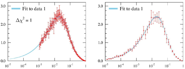
To compare the different reweighting methods we invoke a simple example by constructing two sets of pseudodata for a function $g(x)=a_{0}x^{a_{1}}(1-x)^{a_{2}}e^{xa_{3}}(1+xe^{a_{4}})^{a_{5}},$ shown in Figure 1. We use the first one to construct a set of “Hessian PDFs” as outlined in Section 2 (using the same functional form for $g(x)$) with a chosen tolerance $\Delta\chi^{2}$. Then we take the second data set, work out the predictions of the reweighting methods and compare those to a direct fit including both of these data sets.

Figure 1: Left-hand panel: Pseudodata (data set 1) used to construct the baseline fit. Right-hand panel: Pseudodata (data set 2) used in reweighting.

Figure 2: Left-hand panel: Results of reweighting normalized to to the direct re-fit in the case $\Delta\chi^{2}=1$. Middle panel: As the left-hand panel but for $\Delta\chi^{2}=5$. Right-hand panel: As the middle panel but rescaling by $\Delta\chi^{2}=5$ when computing the Bayesian weights.

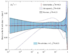
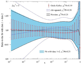
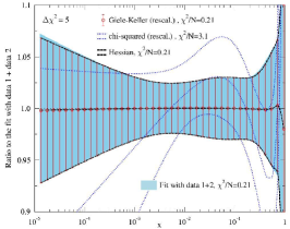
The results of this exercise are shown in Figure 2. We observe that in the case $\Delta\chi^{2}=1$ the Hessian and Giele-Keller reweighting are in perfect agreement with the direct fit (left-hand panel). If we increase the tolerance to $\Delta\chi^{2}=5$, the Hessian procedure still accords with the direct fit but the Giele-Keller method appears to fail (middle panel). However, the agreement can be easily restored by rescaling the values of $\chi^{2}_{k}$ in Eq. (14) as $\chi^{2}_{k}\rightarrow\chi^{2}_{k}/\Delta\chi^{2}$ (left-hand panel). In all cases the Bayesian weights which have been shown to work for the NNPDF-style fits (the chi-squared weights) yield clearly different results.

5 CTEQ6.6 and inclusive jets at the LHC

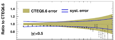
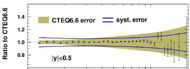
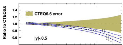
Having now understood how to correctly reweight Hessian PDFs, we illustrate what would be the effect of LHC inclusive jet data on the CTEQ6.6 PDFs [11] (for which which $\Delta\chi^{2}=100$). Specifically, we focus on the $7\,{\rm TeV}$ jet measurements by the CMS collaboration [12] and use the FASTNLO interface [13, 14, 15] for the computations. Before the reweighting CTEQ6.6 tends to somewhat overpredict the experimental cross sections as shown in Figure 3 (left-hand panel) which, however, largely disappears after applying the correlated systematic shifts (right-hand panel). Initially, $\chi^{2}/N\approx 2.1$ (for $N=133$ data points).

Figure 3: Left-hand panel: The CMS jet data (only the midrapidity bin) normalized by the predictions of CTEQ6.6. Right-hand panel: As the left-hand panel but after applying the systematic shifts.

Figure 4: The new gluon PDFs normalized to CTEQ6.6.

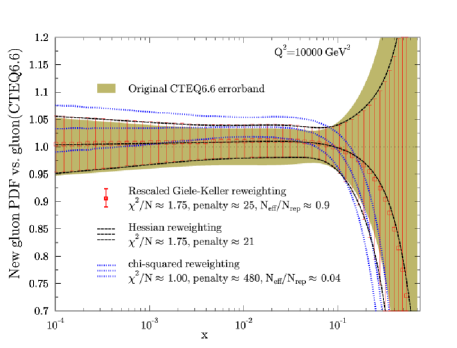
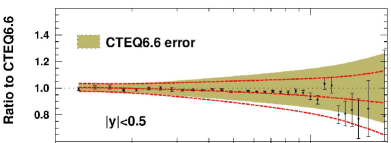
The gluon distributions after applying the reweighting procedures are presented in Figure 4 revealing a decrease in the large-$x$ gluon PDF. As expected, the Hessian and (rescaled) Giele-Keller reweighting agree and only a modest penalty of $\sim~{}20$ units is induced. The new global $\chi^{2}$ has changed by $21-(2.1-1.75)\times 133\approx-30$ units. The result of Bayesian reweighting with chi-squared weights is shown for comparison and a similar but much too pronounced effect is observed. In fact, instead of decreasing, the new global $\chi^{2}$ has increased by $480-(2.1-1.0)\times 133\approx 330$ units. This is also reflected in the new cross-section predictions shown in Figure 5: While the Hessian reweighting (left-hand panel) predicts only a modest decrease in the cross sections (moderating the overshooting observed in Figure 5), the Bayesian reweighting with chi-squared weights (right-hand panel) would lead us to believe in much larger effect.

Figure 5: Left-hand panel: The jet cross sections after the Hessian reweighting (red lines) normalized by the central CTEQ6.6 predictions. The systematic shifts corresponding to the reweighted PDFs have been applied to the data. Right-hand panel: As the left-hand panel but using the Bayesian reweighting with chi-squared weights.

6 Summary

We have discussed how to estimate the effects that a new set of data would have on a global Hessian PDF fit with fixed tolerance $\Delta\chi^{2}$. By considering a simple example, we find that there are two alternative techniques that give essentially the same answer and are equivalent to a direct refit: the Hessian reweighting and a Bayesian technique with rescaled Giele-Keller weights. As a practical example, we employed these methods in the case of inclusive jet production at the LHC.

References

- [1] A. Sapronov, PoS EPS -HEP2013 (2014) 455.
- [2] S. Chatrchyan et al. [CMS Collaboration], arXiv:1312.6283 [hep-ex].
- [3] CMS Collaboration [CMS Collaboration], constant from the inclusive jet cross section at 7 TeV,” CMS-PAS-SMP-12-028.
- [4] R. D. Ball et al. [NNPDF Collaboration], Nucl. Phys. B 849 (2011) 112 [Erratum-ibid. B 854 (2012) 926] [Erratum-ibid. B 855 (2012) 927] [arXiv:1012.0836 [hep-ph]].
- [5] R. D. Ball, V. Bertone, F. Cerutti, L. Del Debbio, S. Forte, A. Guffanti, N. P. Hartland and J. I. Latorre et al., Nucl. Phys. B 855 (2012) 608 [arXiv:1108.1758 [hep-ph]].
- [6] G. Watt, R. S. Thorne, JHEP 1208 (2012) 052 [arXiv:1205.4024 [hep-ph]].
- [7] H. Paukkunen and C. A. Salgado, Phys. Rev. Lett. 110 (2013) 21, 212301 [arXiv:1302.2001 [hep-ph]].
- [8] H. Paukkunen and P. Zurita, arXiv:1402.6623 [hep-ph].
- [9] J. Pumplin, D. Stump, R. Brock, D. Casey, J. Huston, J. Kalk, H. L. Lai, W. K. Tung, Phys. Rev. D 65 (2001) 014013 [hep-ph/0101032].
- [10] W. T. Giele and S. Keller, Phys. Rev. D 58 (1998) 094023 [hep-ph/9803393].
- [11] P. M. Nadolsky, H. -L. Lai, Q. -H. Cao, J. Huston, J. Pumplin, D. Stump, W. -K. Tung and C. -P. Yuan, Phys. Rev. D 78 (2008) 013004 [arXiv:0802.0007 [hep-ph]].
- [12] S. Chatrchyan et al. [CMS Collaboration], Phys. Rev. D 87 (2013) 112002 [arXiv:1212.6660 [hep-ex]].
- [13] T. Kluge, K. Rabbertz and M. Wobisch, hep-ph/0609285.
- [14] D. Britzger et al. [fastNLO Collaboration], arXiv:1208.3641 [hep-ph].
- [15] M. Wobisch et al. [fastNLO Collaboration], arXiv:1109.1310 [hep-ph].