Tackling Radio Polarization of Energetic Pulsars

Abstract

The traditional, geometrical rotating vector model (RVM) has proved particularly poor at capturing the polarization sweeps of the young energetic and millisecond pulsars detected by Fermi. We augment this model by including finite altitude effects using a swept back vacuum dipole geometry. By further including the effects of orthogonal mode jumps, multiple emission altitudes, open zone growth via y-point lowering, and interstellar scattering, we show that a wide range of departures from RVM can be modeled well while retaining a geometrical picture. We illustrate these effects by fitting six Fermi-detected pulsars (J0023$+$0923, J1024$-$0719, J1744$-$1134, J1057$-$5226, J1420$-$6048, and J2124$-$3358) and we describe how such modeling can improve our understanding of their emission geometry.

1. Introduction

For pulsars emitting in the radio, the conventional assumption is that the electric vector position angle follows the projection onto the plane of the sky from the magnetic field line at the emission point. Polarization position angle curves (position angle versus pulsar phase), which we see as the pulsar sweeps past our field of view, are very closely related to the orientation of the magnetic field lines. Analysis of radio polarization is a powerful tool for understanding the geometry of pulsars. For example, polarization contains information about the phase of closest approach of the surface dipole axis. Additionally, polarization has traditionally been used to place strong constraints on the impact angle, the angle between the magnetic pole of the pulsar, and the viewing direction. Modeling polarization should also give estimates for the geometric parameters $\alpha$, the angle of magnetic axes, and $\zeta$, the viewing angle.

Naively, such projections should result in smooth polarization curves versus the pulsar period phase, particularly when adopting a point dipole model. We argue that zero altitude models are not appropriate for certain pulsars. In stark contrast, a relatively recent paper Yan et al. (2011) exhibits the multitude of shapes that occur in millisecond pulsar polarization. More subtly, both polarization angle sweeps originating from zero altitude and polarization angle sweeps originating from a single, finite altitude can differ significantly in shape, although both appear smooth. Emission from finite altitude is a consideration for both millisecond pulsars and young pulsars. Karastergiou & Johnston (2007) give the emission altitude of young pulsars as $950$–$1000$ km. This emission altitude is then $0.02\times 1000/P_{\rm{ms}}$ $R_{\rm{LC}}$ in terms of the light cylinder radius. The light cylinder radius, $R_{\rm{LC}}$, is the distance from the center of the neutron star at which co-rotating particles would be traveling at the speed of light. Since $P_{\rm{ms}}<100$ ms for young pulsars, their emission altitude would be $>0.2R_{\rm{LC}}$, a significant fraction of the light cylinder. The neutron star radius in terms of light cylinder is $0.02\times 10/P_{\rm{ms}}$ $R_{\rm{LC}}$ for a neutron star radius of $10$ km. For millisecond pulsars with $P_{\rm{ms}}<5$ ms, emission must come from $>0.04R_{\rm{LC}}$, which is also a significant fraction of the light cylinder.

Precise modeling of millisecond pulsar and young pulsar radio polarization is of particular interest now because of the growth of $\gamma$-ray data from the Fermi Gamma-Ray Space Telescope. These energetic pulsars make up the $\gamma$-ray pulsar population. Thus, the understanding of $\gamma$-ray models can potentially benefit from radio polarization modeling because of the constraints on geometry that polarization often provides. All pulsars considered in this paper are Fermi-detected pulsars.

In essence, the present paper is an extension of the Karastergiou (2009) paper in which the author shows one can produce theoretical polarization curves similar to those observed using orthogonal mode jumps and interstellar scattering. Here, we also allow for emission from finite altitude (numerically calculated). Although analytically calculated modifications exist for small altitude emission, such calculations contain estimates that break down at altitudes $\sim 0.1R_{\rm{LC}}$. Our model also allows for multiple altitudes of emission. Differences in altitude can explain non-$90^{\circ}$ position angle jumps seen particularly in millisecond pulsar polarization data. Another major difference between Karastergiou (2009) and the present paper is that we seek to quantitatively fit the model to the data resulting in parameters with error bars and $\chi^{2}$ estimates. In contrast, Karastergiou (2009) was satisfied with producing polarization sweeps that appeared qualitatively similar to the data. Further, using the F-test, we compare the $\chi^{2}$ of the simplistic point dipole model and our more complex model to statistically quantify whether the modifications are significant. This paper is a methods paper that chooses pulsars that can clearly illustrate the strengths of this model; we do not tackle a large sample.

In Section 2 of this paper, we discuss the rotating vector model (RVM) and how the discrepancies between data and the model demand a reevaluation of RVM. In Section 3, we describe the constituents of the model in detail. In Section 4, we describe the nuances of fitting the model. Section 4.1 focuses on a parameter $\rho_{\rm{ypt}}$ which we define and use heavily in this paper and which is a measure of the extent of the effective open zone required by phase of emission. We apply the model to data in Section 5. Table 1 gives property parameters to the pulsars analysed.

2. Rotating Vector Model and Beyond

We will start by discussing the analytic models used for radio position angle polarization and their shortcomings and then transition into the numerical model used for this paper. The model predominately used for radio position angle polarization is the RVM which was formulated by Radhakrishnan & Cooke (1969). The RVM is simple and states that pulsars are point dipoles with emission from the surface of the neutron star. The analytic RVM formula for polarization angles ($\psi$) is

$$\psi=\arctan\left[\frac{-\sin(\alpha)\sin(\phi+\Delta\phi)}{\sin(\zeta)\cos(\alpha)-\cos(\zeta)\sin(\alpha)\cos(\phi+\Delta\phi)}\right]+\Delta\psi,$$ (1)

where the inclination angle between the rotation axis and magnetic axis is $\alpha$, the viewing angle is $\zeta$, and the pulse phase is $\phi$. Measures of horizontal and vertical offset are contained in $\Delta\psi$ and $\Delta\phi$. These are the absolute phase and position angle on the sky of the magnetic axis.

Table 1Property Parameters of the Pulsars

Name	Period	$R_{\rm{LC}}/R_{\rm{NS}}$	$f$	DM
	(ms)		(GHz)	(cm-3 pc)
J0023$+$0923	3.05	12.5	1.649	14.326
J1024$-$0719	5.162	20.0	1.369	6.49
J1057$-$5226	197.11	1000	1.5	30.1
J1744$-$1134	4.075	16.7	1.369	3.14
J1420$-$6048	68	250	1.5 and 3	360
J2124$-$3358	4.931	20.0	1.369	4.60

Despite its simplicity, the RVM has been applied to numerous pulsars with great success (i.e., Lyne & Manchester, 1988; Phillips, 1990; Everett & Weisberg, 2001). These pulsars are generally old, spun-down pulsars with long periods and low altitudes of emission. Blaskiewicz et al. (1991) (the Blaskiewicz, Cordes, & Wassermann, or BCW model) modified the RVM to include finite altitude and found that the point of fastest change in the polarization position angle sweep will shift back in phase due to sweep-back effects on the magnetic field lines, while the intensity profile shifts forward in phase due to co-rotation of the particles in the pulsar magnetosphere. Therefore, by fitting the position angle data to the RVM and measuring this shift, one can estimate altitude.

The BCW formula with altitude ($r$) dependence measured in $R_{\rm{LC}}$ is given by

$$\psi=\arctan\left[\frac{-\sin(\alpha)\sin(\phi-2r)}{\sin(\zeta)\cos(\alpha)-\cos(\zeta)\sin(\alpha)\cos(\phi-2r)}\right]+\Delta\psi$$ (2)

(Dyks, 2008).

Figure 1.— Plot of model pulsar intensity and polarization sweep showing the effects of single and multiple altitudes with a small scattering constant. The model parameters are $\alpha=145^{\circ}$, $\zeta=140^{\circ}$, $P=5$ ms, and $\tau=0.03$ ms. The black points are polarization position angles for a model with $R_{1}=0.1R_{\rm{LC}}$ for polarization associated with intensity component $C_{1}$ and $R_{2}=0.1R_{\rm{LC}}$ plus an orthogonal mode jump for polarization associated with intensity component $C_{2}$. The red points are polarization position angles for a model with $R_{1}=0.1R_{\rm{LC}}$ for polarization associated with intensity component $C_{1}$ and $R_{2}=0.15R_{\rm{LC}}$ plus an orthogonal mode jump for polarization associated with intensity component $C_{2}$. Each model polarization sweep for a given component is weighted using the Gaussian intensity profile. Subtle changes in altitude can create drastic changes in the direction of the bridging polarization in the phase of orthogonal mode jump. The two Gaussian components of model intensity are equal in amplitude but interstellar scattering effects make the first Gaussian component in phase ($C_{1}$) slightly lower in amplitude compared with the second Gaussian component in phase ($C_{2}$). A phase of zero is the point of closest encounter to the magnetic axis in the model.

Figure 2.— Panels (A) and (B) show pulsar magnetic field lines at various viewing angles for a pulsar with $\alpha=45^{\circ}$. The magenta lines are the last closed field lines of a vacuum dipole and the solid blue lines represents the light cylinder ($1R_{\rm{LC}}$). Formally, for the vacuum dipole model, the y-point radius ($\rho_{\rm{ypt}}$), the cylindrical radius from the spin axis at which the closed and open field lines are adjacent, is $\rho_{\rm{ypt}}=1R_{\rm{LC}}$. In reality, due to finite mass and current effects, $\rho_{\rm{ypt}}<1R_{\rm{LC}}$. Also plotted is the last closed field lines for $\rho_{\rm{ypt}}=0.7R_{\rm{LC}}$ and $\rho_{\rm{ypt}}=0.4R_{\rm{LC}}$. The inset plot of panel (B) shows a close-up of the y-point area and illustrates why this point is called the y-point. Panel (C) shows a typical model polarization sweep with $\alpha=145^{\circ}$, $\zeta=140^{\circ}$, and $R=0.1R_{\rm{LC}}$. Open circles mark the expected emission phase for the model. Decreasing $\rho_{\rm{ypt}}$ increases the phase of emission. A phase of zero is the point of closest encounter to the magnetic axis in the model.

The formula is approximate and breaks down as altitude increases. The breakdown occurs between $\sim 0.05R_{\rm{LC}}$ and $\sim 0.12R_{\rm{LC}}$ at best, below or near altitudes expected for energetic young and millisecond pulsars. One can apply correction formulae to boost the break-down altitude to $\sim 0.3R_{\rm{LC}}$, but even these formulae are sensitive to $\alpha$ and $\zeta$ and depend on an assumed radio intensity model (Craig & Romani, 2012). In essence, neither the RVM nor the BCW captures the morphological changes in the radio polarization position angle sweep at high altitudes which are needed to model high-energy, $\gamma$-ray emitting pulsars.

Further, the RVM produces smooth S-shaped position angle sweeps versus phase that resemble data from older, low-energy pulsars. Polarization position angle data from millisecond pulsars, on the other hand, are riddled with jumps, cusps, and sharp turns (i.e., Yan et al., 2011; Everett & Weisberg, 2001) which are absent in the RVM (the strongest evidence that the RVM lacks essential physical features needed to understand emission from these pulsars). By combining four physically motivated, data-driven ingredients (numerically calculated finite altitude, multiple altitudes, orthogonal mode jumps, and interstellar scattering), we hope to explain some of the features seen in the radio data of Fermi pulsars for which the RVM alone fails.

In the model presented in this paper, and in contrast to the RVM and the BCW, finite altitude polarization is calculated using numerical computation, which avoids the approximations needed in the BCW. The retarded dipole presented in Kaburaki (1980) and used in Watters & Romani (2011) is used in this modeling. Particles follow magnetic field lines to a given altitude of emission (as measured radially from the center of the neutron star) and, similar to the RVM, radiate tangent to the field line. Co-rotation and time-of-flight effects are then applied when emission from the lab frame is projected onto the plane of the sky (that is, $\psi=\psi_{v}+(|\boldsymbol{\Omega}|/c)\boldsymbol{r}\cdot\hat{k}$ where $\psi$ is the pulsar phase, $\psi_{v}$ is the co-rotational velocity in the $\hat{\psi}$ direction, $\boldsymbol{r}$ is the origin of the emitted photon, and $\hat{k}$ is the direction of the photon motion in the co-rotation frame). The numerical model is particularly valid at lower altitudes of emission and we will often favor fits to the model with low altitude results. High altitude emission requires a force-free model. We ignore magnetospheric charge and current present in force-free models, implicitly assuming that such effects occur at higher altitudes than considered here.

The numerical model does not include the superposition of multiple emission heights which would result in caustics; the altitudes are defined by a single radial distance from the center of the neutron star. The numerical model does not include cross-drift of particles or higher-order multipoles.

3. adding physical ingredients

3.1. Multiple Altitudes

In order to include multiple altitudes, we invoke the patchy cone model (Lyne & Manchester, 1988; Karastergiou & Johnston, 2007), which holds that different components of the pulsar intensity profile come from different areas of the magnetosphere, and hence, different altitudes. The polarized intensity is modeled by a combination of Gaussian profiles. The Gaussian profiles are modeled after those used in Karastergiou (2009). Each Gaussian component or set of Gaussian components is assigned an altitude ($R_{1}$, $R_{2}$, etc.). We used as few altitudes as will result in a reasonable fit and multiple components often have a single altitude. The Stokes parameters are calculated from the model polarization position angles and these Gaussian components weigh the Stokes parameters $Q$ and $U$ from different altitudes to calculate a single polarization position angle per phase bin:

$$\begin{array}[]{l}Q_{\rm{tot}}(\phi)=\sum\limits_{n}g_{n}(\phi)\cos{(2\psi_{n}(\phi))},\\ \\ U_{\rm{tot}}(\phi)=\sum\limits_{n}g_{n}(\phi)\sin{(2\psi_{n}(\phi))},\\ \\ \psi(\phi)=\frac{1}{2}\arctan\left(\frac{U_{\rm{tot}}(\phi)}{Q_{\rm{tot}}(\phi)}\right)\end{array}$$ (3)

(Karastergiou, 2009). Here $g_{n}(\phi)$ is a Gaussian component and $\psi_{n}(\phi)$ is the model polarization associated with that component.

The allowable altitude range in the model is $R=R_{\rm{NS}}$ (the neutron star radius) to $R=.9R_{\rm{LC}}$. Admittedly, we do not attempt to quantify how high of an emission height is too far from the neutron star surface to apply a vacuum model for predictions of polarization position angles. In all likelihood, there will be a smooth deviation of the polarization predicted by the vacuum model from the actual polarization with increasing model altitude and with strong dependence on $\alpha$, $\zeta$, and the exact location of the emission origin within the magnetosphere. Recent and future studies combining vacuum and force-free models (Kalapotharakos et al., 2012) applied to polarization may hold the key to quantifying this breakdown.

The cone–core model is similar to the patchy cone model but more restrictive. Physically, a cone of emission beams from the pulsar cap, flaring out at higher altitudes (Radhakrishnan & Cooke, 1969). The central part of the intensity pulse profile originates from emission low in the magnetosphere near the neutron star surface and the wings of the intensity pulse profile originates from emission high in the magnetosphere. We do not force a cone–core model when fitting altitude but radio modeling of J0023$+$0923 and J1024$-$0719 favor high altitude–low altitude–high altitude emission (versus phase) based on polarization fitting as discussed in Sections 5.1 and  5.2.

The number of model altitudes used in each fit was motivated by the polarization data. For J0023$+$0923 and J1024$-$0719, we applied two altitude fits since our conjecture is that the “jump” seen in the polarization sweep is from a change in emission altitude (Sections 5.1 and  5.2). For J1057$-$5226 and J1744$-$1134 (Sections 5.3 and 5.4), we applied both one and two altitude fitting schemes. Although a single altitude fit would result in a simpler model, it is not unreasonable to assume that emission from opposite poles or at drastically different pulsar phases originates from different heights. Only one altitude was used in the fitting of the polarization position angle data of J1420$-$6048 because of the single smooth sweep in the data (Section 5.5). Polarization data from J2124$-$3358 (Section 5.6) was fit with more altitudes than reported here but such fits did not drastically change the $\chi_{\rm{min}}^{2}$, the $\chi^{2}$ map, nor the fit altitudes. For the sake of simplicity, we only report the three altitude fit results.

3.2. Interstellar Scattering

Interstellar scattering causes a delay of signal as it travels through the medium of space. The result is a delay of the peak, an exponential tail on the intensity profile, and a flattening of the position angle sweep as polarization information from earlier phases “leaks” into polarization in later phases (e.g., Li & Han, 2003). Scattering can be characterized by a scattering time constant and a scattering kernel:

$$g_{ts}(t-t^{\prime})=\left\{\begin{array}[]{lr}0,&t-t^{\prime}<0,\\ e^{-(t-t^{\prime})/\tau_{s}},&t-t^{\prime}>0\end{array}\right.$$ (4)

(Cronyn, 1970). Other response functions also exist, but this scattering kernel (a thin scattering screen halfway between the source and the observer) is incorporated in the model of this paper. Scattering time constants ($\tau_{s}$) as calculated using the Cordes & Lazio (2002) model are used in the computations but are negligible for all pulsars except for J1420$-$6048 in which scattering time was a free parameter (see Section 5.5 for details).

Adding scattering to position angle polarization is done by convolving the scattering kernel with $Q_{\rm{tot}}(\phi)$ and $U_{\rm{tot}}(\phi)$:

$$\begin{array}[]{l}Q_{\rm{tot}}^{\rm{scat}}(\phi)=\int Q_{\rm{tot}}(\phi(t^{\prime}))g(t-t^{\prime})dt^{\prime},\\ \\ U_{\rm{tot}}^{\rm{scat}}(\phi)=\int U_{\rm{tot}}(\phi(t^{\prime}))g(t-t^{\prime})dt^{\prime}.\end{array}$$ (5)

The resulting $Q_{\rm{tot}}^{\rm{scat}}(\phi)$ and $U_{\rm{tot}}^{\rm{scat}}(\phi)$ are plugged into Equation (3) (bottom line) to obtain polarization. Further, model linear intensity with interstellar scattering is calculated using $\sqrt{Q_{\rm{tot}}^{\rm{scat}}(\phi)^{2}+U_{\rm{tot}}^{\rm{scat}}(\phi)^{2}}$.

3.3. Orthogonal Mode Jumps in the Context of Multiple Altitudes and Interstellar Scattering

The model also includes orthogonal mode jumps in the polarization position angle sweep (Backer et al., 1976). To create orthogonal jumps, $90^{\circ}$ is added to the model polarization position angles ($\psi+90^{\circ}$); Q and U model values can be calculated and used in Equations (3) and (5) the same as unjumped polarization. We do not attempt to understand the origin of these jumps since our model does not contain the physics needed to do so but rather we use the jumps on the basis of empirical observation (e.g., Stinebring et al. 1984; Gould & Lyne 1998; Karastergiou et al. 2005). Note that components of polarized intensity at the same altitude but in different modes will cancel exactly where their individual absolute intensities are equal (Equation (3)). Polarized intensity going to zero at a given phase in the intensity profile indicates an orthogonal mode jump. Further, if the orthogonal mode jump occurs between components of different altitudes, the polarized intensity will not cancel exactly, although in most cases it will be near zero.

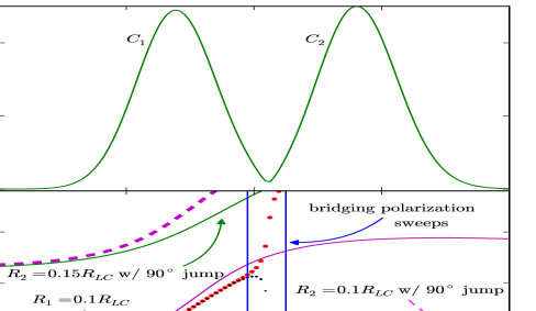
Additionally, without multiple altitudes, only $90^{\circ}$ jumps are allowed and the direction of the bridging polarization position angle sweep between the jump is in the opposite direction from the sweep without the jump. Mathematically, this is due to the forward scattering nature of the scattering kernel. Equation (5) is nonzero only for $t-t^{\prime}>0$ and convolution with such a function will mathematically cause polarization from earlier in phase to mix with polarization at any given phase. Similarly, this is why the second model Gaussian component in phase ($C_{2}$) is higher in intensity than the first ($C_{1}$) in Figure 1.

Figure 1 illustrates some properties of scattering and mode jumps that will be of particular interest in the analysis of fitting J0023$+$0923 and J2124$-$3358 polarization data. An orthogonal mode jump in the position angle sweep between components of the same altitude will result in a bridging sweep with the opposite curvature compared with the unjumped sweep. In the example figure, the magenta solid line has an upward curvature at the jump phase. The resulting curve with the addition of an orthogonal mode jump (black dots) curves downward at the jump phase. This opposite curvature should always occur due to forward scattering if the individual component altitudes are exactly the same. If the component altitudes are not the same, the bridging curvature between the orthogonal polarization position angles could be the same as or opposite the curvature of the original sweep direction depending on the polarization position angles (and Stokes parameters) being combined. This will be an important argument for orthogonal mode jumps between different altitude components in Sections 5.1 and 5.6.

In Figure 1 (along with all subsequent graphs with an $x$-axis of pulsar phase), the phase of zero is the point of closest encounter to the magnetic axis in the model.

4. Fitting Methodology

Simple Gaussian curves were used to model the pulsar intensity. A fixed set of Gaussian phases, widths, and amplitudes drawn by eye that mimic the linear intensity amplitude were used. Formally fitting the pulsar intensity would require simultaneously fitting the polarization position angle parameters and the Gaussian parameters. Such a fit would be computationally intensive and have minimal corrections to the model fits of the polarization.

For the fitting of the polarization position angles, we fit the horizontal and vertical offsets ($\Delta\phi$ and $\Delta\psi$) and altitudes ($R_{1}$, $R_{2}$, etc.) with $\alpha$ and $\zeta$ fixed in $1^{\circ}$ increments. We used a simulated annealing scheme to find the global minimum for a given $\alpha$ and $\zeta$  (Flannery et al., 1992). We then randomly sample the surrounding parameter space within $3\sigma$ of the lowest $\chi^{2}$ for every fixed $\alpha$–$\zeta$ pair to calculate fit error bars.

Phase cuts were applied to the polarization data points where total normalized intensity dropped below $10\%$ for a given pulse. Error bar cuts were also applied to data points where error bars exceeded $\pm 20^{\circ}$. Error bar cuts were chosen such that we had good confidence that data points are within half of the $180^{\circ}$ range that they can occupy (because of the possibility of orthogonal mode jumps). Phase cuts were chosen such that only data points with a reasonable signal-to-noise ratio were considered.

4.1. y-point Considerations

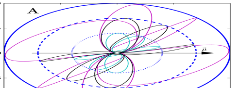
The light cylinder is defined as $R_{\rm{LC}}=cP/2\pi$ where $c$ is the speed of light and $P$ is the period of the pulsar. This cylindrical distance (measured from the neutron star rotation axes) is where particles in co-rotation with the neutron star would be traveling at the speed of light. At this point (or more physically, before this point), the field lines “break open.” These open field lines are where in the magnetosphere particles accelerate and the pulsar radiates. The point at which an open field line is adjacent to a closed field line is the y-point since the adjacent open and closed field lines form a Y in the field (see Figure 2(B) inset for illustration of the y-point). Figure 2 (panels (A) and (B)) plots the field lines of a model pulsar with $\alpha=45^{\circ}$ ($\boldsymbol{\mu}$ is the magnetic axis and the spin axis is vertical). Panel (A) shows a top view of the light cylinder (solid blue lines) while panel (B) shows a side view of the light cylinder. The magenta field lines represent the last closed field lines of a vacuum dipole model with the y-point occurring just beyond the light cylinder.

Studies with force-free simulations (Spitkovsky, 2006) valid at heights near the light cylinder indicate the y-point typically occurs further in than the light cylinder due to particle mass and charge current. The location of the y-point controls the size of the cap of emission from which the open field lines and emission originate. Smaller $\rho_{\rm{ypt}}$, the cylindrical distance of the y-point from the neutron star, results in a larger cap, a wider range of viewing angles over which emission can be seen, and a wider phase over which emission is produced. Often, the emission phase in data is too large to be accommodated by the open zone of the formal vacuum dipole even with finite altitude; this is evidence that the field lines break open further in from the light cylinder. The cyan and black field lines in Figure 2 illustrate the location and form of the last closed field lines with the y-point distance equal to $\rho_{\rm{ypt}}=0.4R_{\rm{LC}}$ or $\rho_{\rm{ypt}}=0.7R_{\rm{LC}}$ respectively.

Panel (C) of Figure 2 shows the effect of a shifted y-point on the range of emission allowed from open field lines. Panel (C) is a plot of a typical model polarization position angle sweep with $\alpha=145^{\circ}$, $\zeta=140$, and $R=0.1R_{\rm{LC}}$. The open circles mark the region in phase where emission is allowed for various $\rho_{\rm{ypt}}$. As $\rho_{\rm{ypt}}$ decreases, the allowed range of emission increases.

In the modeling for this paper, emission is treated as coming from all field lines not just those defined as open by the formal cap using the light cylinder distance. Polarization data are fit without constraints from the emission phase. We then report the $\rho_{\rm{ypt}}$ needed for the entire phase of emission seen in the intensity data to be covered by model data in the same phase.

5. Application (and illustration) with Individual Pulsars

5.1. J0023$+$0923: Nonorthogonal Jumps with Multiple Altitudes

Table 2Fit Parameters for J0023$+$0923

	DOF	(Unreduced) $\chi^{2}_{\rm{min}}$	$\alpha$ (∘)	$\zeta$ (∘)	$R_{1}$ ($R_{LC}$)	$R_{2}$ ($R_{LC}$)	$\Delta R$ ($R_{LC}$)
RVM	131-4	$1053$	$8^{+25(+56)}_{-6(-7)}$	$13^{+38(+71)}_{-10(-11)}$	$\cdots$	$\cdots$	$\cdots$
Region A 2 Alt	131-6	$313$	$57^{+15(+53)}_{-14(-30)}$	$105^{+14(+36)}_{-16(-47)}$	$0.67^{+0.23(+0.23)}_{-0.24(-0.43)}$	$0.28^{+0.24(+0.33)}_{-0.14(-0.20)}$	$0.39^{+0.23(+0.35)}_{-0.11(-0.23)}$
Region B 2 Alt	131-6	$324$	$59^{+8(+28)}_{-10(-58)}$	$49^{+2(+7)}_{-5(-48)}$	$0.53^{+0.07(0.17)}_{-0.07(-0.22)}$	$0.90^{+0.00(+0.00)}_{-0.06(-0.27)}$	$-0.37^{+0.08(+0.17)}_{-0.06(-0.22)}$

Figure 3.— In the upper panel, blue points are total radio intensity data at 1.646 GHz, red points are linear polarization intensity data and green points are circular polarization intensity data for J0023$+$0923. The solid magenta line in the upper panel is the model linear intensity used in fitting. In the bottom panel, blue error bars are polarization position angles used in the fit and yellow error bars are polarization position angles excluded by error bar cuts (but not excluded by phase cuts). The model polarization comes from a fit with (unreduced) $\chi^{2}=332$ and parameters $\alpha=59^{\circ}$ and $\zeta=119^{\circ}$. The green solid line is the polarization for a model with $R_{1}=0.77R_{\rm{LC}}$ and the black solid line is the polarization for a model with $R_{2}=0.38R_{\rm{LC}}$. The red solid line is the model polarization of the two altitudes weighted by the model intensity. Empty circles mark the limiting phase of emission from open field lines with $\rho_{\rm{ypt}}=1R_{\rm{LC}}$. A phase of zero is the point of closest encounter to the magnetic axis in the model.

Figure 4.— Map of (unreduced) $\chi^{2}$ for J0023$+$0923 in the $\alpha$–$\zeta$ plane. Cyan contours mark $3\sigma$ from $\chi^{2}_{\rm{min}}$ for fits with $\rho_{\rm{ypt}}=1R_{\rm{LC}}$. This contour contains the lowest values of $\chi^{2}$. The two regions of statistically acceptable fits have drastically different fit parameters.

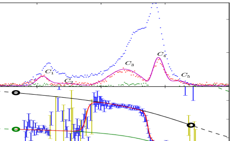
J0023$+$0923 is a Fermi millisecond pulsar with $P=3.05$ ms. Figure 3 shows the radio pulse profile and the polarization position angles at 1.646 GHz. The polarization sweep cannot be explained well using the RVM because of sharp curvature between intensity components $C_{2}$ and $C_{3}$ and between components $C_{3}$ and $C_{4}$. The RVM with an orthogonal mode jump between these components produces more reasonable fits as reported in Table 2. This fit is unsatisfying because the jump is closer to $\sim 60^{\circ}$ rather than $90^{\circ}$. Fitting with an orthogonal mode jump plus two altitudes (one altitude, $R_{1}$, assigned to $C_{1}$, $C_{2}$, $C_{4}$, and $C_{5}$ and a second altitude, $R_{2}$, assigned to $C_{3}$) gives a fit with significantly smaller $\chi^{2}_{\rm{min}}$ (unreduced $\chi^{2}_{\rm{min}}=313$ versus unreduced $\chi^{2}_{\rm{min}}=1053$). By including two physically motivated parameters (the two altitudes), the $\chi^{2}_{\rm{min}}$ is decreased by a factor of three. The $F$-test between the RVM and the two-altitude model gives $F=149.12$, $\rm{DOF}_{1}=2$, and $\rm{DOF}_{2}=125$. The probability of exceeding this $F$ is $\rm{Prob}\sim 0$. This pulsar is an excellent example of how modeling with multiple altitudes can greatly improve $\chi^{2}_{\rm{min}}$ compared to the RVM. It is an example of how multiple altitudes can easily explain a non-$90^{\circ}$ orthogonal mode jumps since components of emission with different altitudes allow for these non-$90^{\circ}$ mode jumps. Figure 3 shows the polarization position angle and intensity data overlaid with the best fit two altitudes plus the orthogonal mode jump model.

Further confirmation that this mode jump is between components from different altitudes in the magnetosphere comes from the curvature direction of the polarization position angle sweep between adjacent modes. The polarization sweep direction between components $C_{3}$ and $C_{4}$ is in the same direction as both the individual unweighted model curves (solid black and red lines). Such a direction of curvature is impossible for a mode jump between equal altitudes as discussed in Section 3.3. Also, such a direction of curvature is impossible in the RVM model which partially accounts for the poor fit.

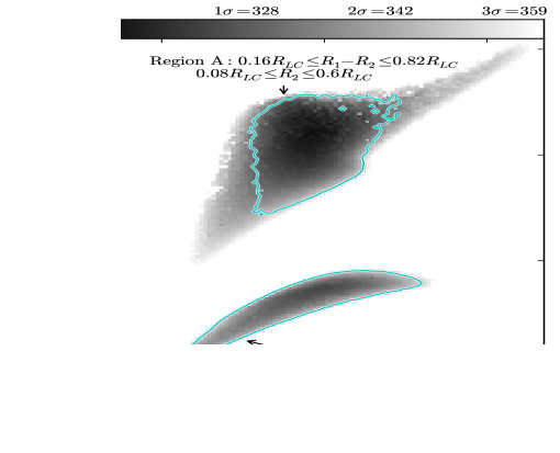
Satisfactory fits exist for both $\rho_{\rm{ypt}}=1R_{\rm{LC}}$ and $\rho_{\rm{ypt}}<R_{\rm{LC}}$. Figure 4 is the (unreduced) $\chi^{2}$ map in the $\alpha$–$\zeta$ plane and the thin cyan contour represents the allowable area up to $3\sigma$ from $\chi^{2}_{\rm{min}}$ in which the emission comes only from the formal open field line region of the magnetic pole as defined by $\rho_{\rm{ypt}}=1R_{\rm{LC}}$. The minimum $\chi^{2}$ region is well within the $\rho_{\rm{ypt}}=1R_{\rm{LC}}$ region as seen from Figure 4. Also Figure 3 shows a polarization position angle model that emits over the entire phase of emission seen in the data where the circles on the plot mark the phase defining the formal open zone for the two altitudes of emission used in the model.

In the $\alpha$–$\zeta$ plane, two islands of acceptable regions of $\chi^{2}<3\sigma$ arise as seen in Figure 4. Parameters and errors for each of these sections are reported separately in Table 2. The distinguishing parameter between these two regions is $R_{2}$. For the region between $\zeta=1^{\circ}$ and $\zeta=56^{\circ}$, $R_{2}=0.63$–$0.90R_{\rm{LC}}$. For the region between $\zeta=58^{\circ}$ and $\zeta=141^{\circ}$, $R_{2}=R_{\rm{ns}}=0.08$–$0.61R_{\rm{LC}}$. The region between $\zeta=58^{\circ}$ and $\zeta=141^{\circ}$ is more plausible for our model because it favors lower altitudes. Additionally, $\Delta R=R_{1}-R_{2}$ for this region is positive and favors the cone–core model discussed previously (see Table 2 for values).

5.2. J1024$-$0719: Kinks with Multiple Altitudes

Table 3Fit Parameters for J1024$-$0719

		(Unreduced)
	DOF	$\chi^{2}_{\rm{min}}$	$\alpha$ (∘)	$\zeta$ (∘)	$R_{1}$ ($R_{\rm{LC}}$)	$R_{2}$ ($R_{\rm{LC}}$)	$\Delta R$ ($R_{\rm{LC}}$)	$\Delta\rho$ ($R_{\rm{LC}}$)	$\rho_{\rm{ypt}}$ ($R_{\rm{LC}}$)
RVM	397-4	$8963$	$98^{+1(+3)}_{-3(-4)}$	$87^{+1(+2)}_{-2(-2)}$	$\cdots$	$\cdots$	$\cdots$	$\cdots$	$\cdots$
Region A 2 Alt	397-6	$3409$	$112^{+1(+2)}_{-1(-3)}$	$63^{+2(+5)}_{-3(-6)}$	$0.90^{+0.00(+0.00)}_{-0.02(-0.05)}$	$0.82^{+0.00(+0.01)}_{-0.02(-0.05)}$	$0.08^{+0.01(+0.01)}_{-0.00(-0.01)}$	$0.11^{+0.00(+0.01)}_{-0.01(-0.01)}$	$1.00^{+0.00(+0.00)}_{-0.02(-0.04)}$
Region B 2 Alt	397-6	$3447$	$113^{+1(+4)}_{-1(-4)}$	$108^{+1(+4)}_{-1(-4)}$	$0.22^{+0.01(+0.04)}_{-0.03(-0.05)}$	$0.05^{+0.00(+0.01)}_{-0.00(-0.00)}$	$0.17^{+0.01(+0.04)}_{-0.03(-0.05)}$	$0.04^{+0.01(+0.08)}_{-0.01(-0.03)}$	$0.24^{+0.00(+0.07)}_{-0.02(-0.04)}$

Figure 5.— In the upper panel, blue points are total radio intensity data for 1.369 GHz, red points are linear polarization intensity data, and green points are circular polarization intensity data for J1024$-$0719. The solid magenta line in the upper panel is the model linear intensity used in fitting. In the bottom panel, blue error bars are polarization position angles used in the fit and yellow error bars are polarization position angles excluded by error bar cuts (but not excluded by phase cuts). The model polarization comes from a fit with (unreduced) $\chi^{2}=3448$ and parameters $\alpha=113^{\circ}$ and $\zeta=108^{\circ}$. The green solid line is the polarization for a model with $R_{1}=0.22R_{\rm{LC}}$ and the black solid line is the polarization for a model with $R_{2}=0.05R_{\rm{LC}}$. The red solid line is the model polarization of the two altitudes weighted by the model intensity. Empty circles mark the limiting phase of emission from open field lines with $\rho_{\rm{ypt}}=1R_{\rm{LC}}$. Solid lines mark the allowed emission phase for an effective open zone with $\rho_{\rm{ypt}}=0.24R_{\rm{LC}}$ which is required for the model phase to cover the entire emission phase in the data. A phase of zero is the point of closest encounter to the magnetic axis in the model.

Figure 6.— Map of (unreduced) $\chi^{2}$ for J1024$-$0719 in the $\alpha$–$\zeta$ plane for Regions A and B. The regions vary drastically from one another in parameters although they are comparable in $\chi^{2}$. Both are very restrictive in their respective parameters.

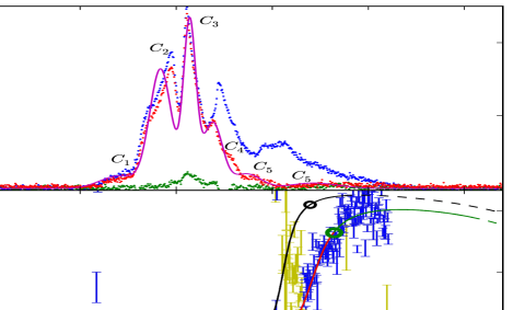
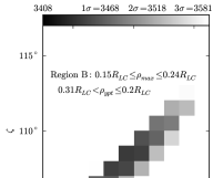
J1024$-$0719 is another millisecond Fermi-detected pulsar ($P=5.162$ ms). This pulsar fits reasonably well to the RVM (1.369 GHz data shown in Figure 5) although certain features in the polarization data are highly statistically significant and unexplained by the RVM. Most notably, a kink in the polarization occurs in the transition from intensity component $C_{2}$ to $C_{3}$ and from $C_{4}$ to $C_{5}$ (as labeled on Figure 5). Similar to J0023$+$0923, this jump can be modeled using multiple altitudes, modeling the kink as the shift in altitude between the emission components. The error bars on this model are fairly small for the fit parameters (Table 3) since a limited number of parameter combinations make a sweep with this particular polarization difference with two heights. Additionally, the data contains the polarization at the point of closest encounter to the magnetic axis (the fastest change in the sweep) which also greatly constrains the fitting parameters. Overall, this pulsar is another excellent example of how using multiple altitudes can explain features not found in the RVM.

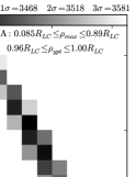
Similar to J0023$+$0923, two regions arise in the $\alpha$–$\zeta$ plane of the (unreduced) $\chi^{2}$ map (see Figure 6) that are statistically acceptable. For the two regions, the altitudes are significantly different and are reported separately in Table 3.

In Region A, the $\rho_{\rm{ypt}}$ needs to be $0.22R_{\rm{LC}}\leq\rho_{\rm{ypt}}\leq 0.34R_{\rm{LC}}$ in order to account for the full phase of the emission and remain within $3\sigma$ of $\chi^{2}_{\rm{min}}$. Figure 5 displays the model polarization sweep from this region. The green and black circles represent the limiting phase of emission defined by the formal cap with $\rho_{\rm{ypt}}=1R_{\rm{LC}}$. The solid lines mark the effective open zone emission for $\rho_{\rm{ypt}}=0.24R_{\rm{LC}}$. Both sets of circles are well within the limiting phase of emission seen in the data. For most of the models within $3\sigma$ of $\chi^{2}_{\rm{min}}$, the emission phase of the outer altitude ($R_{1}$ represented by the green line in Figure 5) controls the location of $\rho_{\rm{ypt}}$. For Region A, $R_{1}=0.14$–$0.26R_{\rm{LC}}$, $R_{2}=0.05$–$0.06R_{\rm{LC}}$. The outer emission altitude, $R_{1}$, is typically larger than the inner emission altitude, $R_{2}$, which is consistent with a cone–core model similar to the two fit altitude parameters for the polarization position data from J0023$+$0923 .

For Region B, the $\rho_{\rm{ypt}}$ is much higher than that in Region A but likewise so are $R_{1}$ and $R_{2}$. Approximately $\rho_{\rm{ypt}}=0.96$–$1.0R_{\rm{LC}}$, $R_{1}=0.85$–$0.9R_{\rm{LC}}$, $R_{2}=0.77$–$0.83R_{\rm{LC}}$. Although $\rho_{\rm{ypt}}$ is much larger in Region B than in Region A, the altitude of emission is also close to $R_{\rm{LC}}$ resulting in a $\Delta\rho=\rho_{\rm{ypt}}-\rho_{\rm{max}}$ (the difference between the y-point cylindrical distance needed to open up the field lines to the appropriate amount to accommodate the emission phase in the data and the maximum cylindrical distance of the emission within this phase) similar to that of Region A. Additionally, $\Delta\rho$ is relatively small (see Table 3). This is problematic because we expect emission this close to the light cylinder to resemble a force-free model and to be dictated by physics that we do not include in the vacuum model. To explain the phase of emission seen in the data using this model, one must either push the altitude up to extreme heights or accept $\rho_{\rm{ypt}}$ much smaller than $1R_{\rm{LC}}$.

J1024$-$0719 is modeled with two altitudes, one altitude component inside the other in terms of phase, making it a good candidate for the cone–core model. The parameter $\Delta R=R_{1}-R_{2}$ (where $R_{1}$ is the altitude associated with component $C_{1}$, $C_{5}$, and $C_{6}$ and $R_{2}$ is the altitude associated with $C_{2}$ and $C_{3}$) should be positive in the case of a cone–core model. Table 3 shows this value to be positive for both Regions A and B. Further, to $3\sigma$, these values are positive and radio modeling of J1024$-$0719 polarization is consistent with the cone–core model.

For the RVM (unreduced) $\chi^{2}_{\rm{min}}=8963$ and for the two-altitude model (unreduced) $\chi^{2}_{\rm{min}}=3408$. By including two physically motivated parameters, the $\chi^{2}_{\rm{min}}$ is decreased by a factor of three. The $F$-test between the RVM and the two-altitude model gives $F=318.66$, DOF${}_{1}=2$, and DOF${}_{2}=391$. The probability of exceeding this $F$ is Prob$\sim 0$. By these statistical measures, a two-altitude model is clearly better than the RVM.

5.3. J1057$-$5226: y-point and Finite Altitude

Table 4Fit Parameters for J1057$-$5226

		(Unreduced)
	DOF	$\chi^{2}_{\rm{min}}$	$\alpha$ (∘)	$\zeta$ (∘)	$R_{1}$ ($R_{\rm{LC}}$)	$R_{2}$ ($R_{\rm{LC}}$)	$\Delta\rho$ ($R_{\rm{LC}}$)	$\rho_{\rm{max}}$ ($R_{\rm{LC}}$)	$\rho_{\rm{ypt}}$ ($R_{\rm{LC}}$)
RVM	166-4	$325$	$77^{+0(+1)}_{-1(-1)}$	$70^{+0(+0)}_{-0(-0)}$	$\cdots$	$\cdots$	$\cdots$	$\cdots$	$\cdots$
1 Alt	166-5	$282$	$76^{+2(+2)}_{0(-1)}$	$64^{+5(+5)}_{-34(-35)}$	$0.19^{+0.43(+0.46)}_{-0.12(-0.13)}$	$\cdots$	$\cdots$	$\cdots$	$\cdots$
2 Alt	166-6	$281$	$69^{+14(+26)}_{-4(-9)}$	$64^{+5(+6)}_{-37(-39)}$	$0.12^{+0.72(+0.72)}_{-0.06(-0.12)}$	$0.31^{+0.59(+0.59)}_{-0.29(-0.31)}$	$0.15^{+0.32(+0.40)}_{-0.15(-0.15)}$	$0.31^{+0.36(+0.52)}_{-0.25(-0.28)}$	$0.46^{+0.54(+0.54)}_{-0.40(-0.40)}$

Figure 7.— In the upper panel, blue points are total radio intensity data for 1.5 GHz, red points are linear polarization intensity data, and green points are circular polarization intensity data for J1057$-$5226. The solid magenta line in the upper panel is the model linear intensity used in fitting. In the bottom panel, blue error bars are polarization position angles used in the fit and yellow error bars are polarization position angles excluded from the fit because of phase cuts (see text). The model polarization comes from a fit with (unreduced) $\chi^{2}=289$ and parameters $\alpha=77^{\circ}$ and $\zeta=30^{\circ}$. The green solid line is the polarization for a model with $R_{1}=0.58R_{\rm{LC}}$ and the black solid line is the polarization for a model with $R_{2}=0.63R_{\rm{LC}}$. The red solid line is the model polarization of the two altitudes. Empty circles mark the limiting phase of emission from open field lines with $\rho_{\rm{ypt}}=1R_{\rm{LC}}$. Solid lines mark allowed emission phase for an effective open zone with $\rho_{\rm{ypt}}=0.71R_{\rm{LC}}$ ($\Delta\rho=0.49R_{\rm{LC}}$) which is required for the model phase to cover the entire emission phase in the data. A phase of zero is the point of closest encounter to the magnetic axis in the model.

Figure 8.— Map of (unreduced) $\chi^{2}$ for J1057$-$5226 in the $\alpha$–$\zeta$ plane with $3\sigma$ contours for sets of $\rho_{\rm{max}}$ ranges, the single altitude model fit, and $\Delta\rho>0.2R_{\rm{LC}}$. The best fit for the RVM is also indicated on the map. The best fit using the RVM is quite different from the best fit using finite altitude and restrictions from the phase of emission seen in the data ($\Delta\rho>0.2R_{\rm{LC}}$).

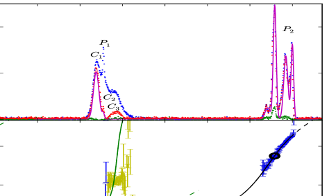
J1057$-$5226 is a relatively young pulsar ($P=197.11$ ms) that has had its radio polarization position angle sweep fit in the literature with the RVM (Weltevrede & Wright, 2009). Here we fit the latest polarization data for J1057$-$5226 at 1.369 GHz with the RVM plus our own finite altitude model. Polarization and intensity data for J1057$-$5226 is plotted in Figure 7. First note that we are unable to explain the polarization position angles associated with $C_{3}$ as labeled in Figure 7 with either the RVM or our current model. This portion of the polarization sweep had not appeared in the previous RVM fitting papers due to poor signal-to-noise. Although we will not attempt to explain this component here, we hope to explore modifications to our current model that will explain this component in future work.

Ignoring the polarization position angles associated with $C_{3}$ for the moment, unlike J0023$+$0923 and J1024$-$0719, J1057$-$5226 does not have any compelling features to indicate mode jumps or multiple altitudes. The $\chi^{2}_{\rm{min}}$ for the RVM even gives a reasonable fit for the number of degrees of freedom (DOF, Table 3). Even so, by fitting to a finite altitude and finite multiple altitudes, we can significantly decrease the $\chi^{2}_{\rm{min}}$ and open the parameter space. Further, Weltevrede & Wright (2009) were forced to conclude that emission comes from outside the formal open zone cap due to the large emission phase of J1057$-$5226. Here we seek a more physical model using a finite altitude and $\rho_{\rm{ypt}}<R_{\rm{LC}}$.

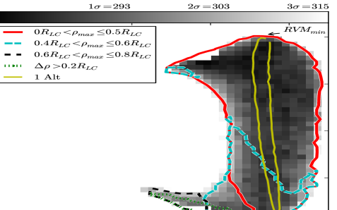
We can model the data with $\rho_{\rm{ypt}}=1R_{\rm{LC}}$ within $1\sigma$ of $\chi^{2}_{\rm{min}}$ but this requires pushing the model to the highest allowed altitudes. On the other hand, low altitudes are also permitted but require low $\rho_{\rm{ypt}}$ in order for the models to emit in the phase observed in the data. The true fit likely lies somewhere between the extremes. A strong correlation exists between $\alpha$, $\zeta$, $R_{1}$, and $R_{2}$ such that if one has an estimated range for $R_{1}$ or $R_{2}$, the acceptable $\alpha$–$\zeta$ models would be significantly decreased.

Red, cyan, and black contours on Figure 8 are $3\sigma$ contours from $\chi^{2}_{\rm{min}}$ of different ranges of $\rho_{\rm{max}}$, the maximum cylindrical distance of the emission within the emission phase for the model. These contours exemplify the correlation between altitude and $\alpha$–$\zeta$ pairs in a single parameter. Further, fits with smaller $\rho_{\rm{max}}$ are more physically likely but so is larger $\Delta\rho$ such as $\Delta\rho>0.2R_{\rm{LC}}$ ($3\sigma$ dashed green contours on Figure 8). As such, one might expect the most physically plausible fits to fall within the green and cyan contours.

The yellow contour is the $3\sigma$ contour from $\chi^{2}_{\rm{min}}$ of a single-altitude model. Going from one altitude to two altitudes does not greatly improve $\chi^{2}_{\rm{min}}$. Adding the additional parameter does allow for a wider variety of geometric configurations ($\alpha$ and $\zeta$) which could be of importance when comparing to multi-wavelength results.

For the RVM (unreduced) $\chi^{2}_{\rm{min}}=325$ and for the two-altitude model (unreduced) $\chi^{2}_{\rm{min}}=281$ (see Table 4). The $F$-test between the RVM and the two-altitude model gives $F=12.50$, DOF${}_{1}=2$, and DOF${}_{2}=160$. The probability of exceeding this $F$ is $P=8.78\times 10^{-6}$. Comparing the RVM to the single-altitude model ($\chi^{2}_{\rm{min}}=282$), the probability of exceeding $F=24.55$ is $\rm{Prob}=1.82\times 10^{-6}$. Comparing the single-altitude model to the two-altitude model, the probability of exceeding $F=0.57$ is $\rm{Prob}=4.52\times 10^{-1}$.

5.4. J1744$-$1134: Multiple Altitudes with Single Versus Double Pole

Table 5Fit Parameters for J1744$-$1134

		(Unreduced)
	DOF	$\chi^{2}_{\rm{min}}$	$\alpha$ (∘)	$\zeta$ (∘)	$R_{1}$ ($R_{\rm{LC}}$)	$R_{2}$ ($R_{\rm{LC}}$)	$\Delta\rho$ ($R_{\rm{LC}}$)	$\rho_{\rm{ypt}}$ ($R_{\rm{LC}}$)
RVM	209-4	$355$	$74^{+0(+1)}_{-2(-4)}$	$97^{+0(+1)}_{-2(-3)}$	$\cdots$	$\cdots$	$\cdots$	$\cdots$
2 Alt no jump	209-6	$311$	$76^{+2(+6)}_{-11(-15)}$	$60^{8(+84)}_{-18(-26)}$	$0.68^{+0.09(+0.18)}_{-0.12(-0.62)}$	$0.70^{+0.20(+0.20)}_{-0.03(-0.64)}$	$0.06^{+0.00(+0.33)}_{-0.04(-0.06)}$	$0.73^{+0.19(+0.27)}_{-0.03(-0.06)}$
2 Alt jump	209-6	$314$	$92^{+2(+4)}_{-53(-70)}$	$57^{+76(+79)}_{-8(-32)}$	$0.87^{+0.03(+0.03)}_{-0.76(-0.81)}$	$0.88^{+0.02(+0.02)}_{-0.24(-0.44)}$	$0.05^{+0.24(+0.27)}_{-0.05(-0.05)}$	$0.81^{+0.19(+0.19)}_{-0.11(-0.37)}$
1 Alt single pole	209-5	$310$	$66^{+5(+15)}_{-4(-7)}$	$85^{+3(+35)}_{-36(-39)}$	$0.65^{+0.07(+0.20)}_{-0.27(-0.54)}$	$\cdots$	$0.36^{+0.09(+0.12)}_{-0.35(-0.47)}$	$0.99^{+0.01(+0.01)}_{-0.50(-0.86)}$
2 Alt single pole	209-6	$309$	$66^{+11(+17)}_{-22(-36)}$	$85^{+24(+32)}_{-53(-60)}$	$0.65^{+0.14(+0.25)}_{-0.55(-0.59)}$	$0.59^{+0.31(+0.31)}_{-0.23(-0.52)}$	$0.37^{+0.19(+0.30)}_{-0.37(-0.37)}$	$1.00^{0.00(+0.00)}_{-0.56(-0.93)}$

Figure 9.— In the upper panels, blue points are total radio intensity data for 1.369 GHz, red points are linear polarization intensity data, and green points are circular polarization intensity data for J1744$-$1134. The solid magenta line in the upper panels is the model linear intensity used in fitting. In the bottom panels, blue error bars are polarization position angles used in the fit. For panel (A), the model polarization comes from a double magnetic pole model with (unreduced) $\chi^{2}=342$, $\alpha=82^{\circ}$, and $\zeta=39^{\circ}$. The green line is the polarization for a model with $R_{1}=0.78R_{\rm{LC}}$ and the black line is the polarization for a model with $R_{2}=0.72R_{\rm{LC}}$. The emission phase from the data for these model parameters requires $\rho_{\rm{ypt}}=0.96R_{\rm{LC}}$ as marked on the plot with the solid lines. For panel (B), the model polarization comes from a single magnetic pole model with (unreduced) $\chi^{2}=317$, $\alpha=66^{\circ}$, and $\zeta=85^{\circ}$. The green solid line is the polarization for a model with $R_{1}=0.65R_{\rm{LC}}$ and the black solid line is the polarization for a model with $R_{2}=0.59R_{\rm{LC}}$. The emission phase from the data is covered with $\rho_{\rm{ypt}}=1R_{\rm{LC}}$ for these model parameters. Empty circles mark the limiting phase of emission from open field lines with $\rho_{\rm{ypt}}=1R_{\rm{LC}}$. A phase of zero is the point of closest encounter to the magnetic axis in the model.

Figure 10.— Map of (unreduced) $\chi^{2}$ for J1744$-$1134 in the $\alpha$–$\zeta$ plane for a single magnetic pole model with $3\sigma$ contours for two $R_{1}$ ranges to show correlation between $\alpha$, $\zeta$, and altitude for $\Delta\rho\leq 0.25R_{\rm{LC}}$ (the more approximate models) and $\rho_{\rm{ypt}}=1R_{\rm{LC}}$ (the less approximate models), and for the single-altitude model which lies mostly in the physically inaccurate contour of $\Delta\rho\leq 0.25R_{\rm{LC}}$ and therefore argues for a two-altitude model.

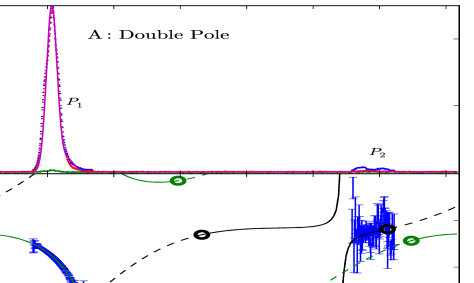
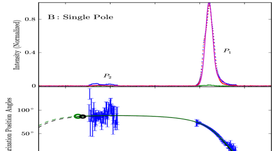
J1744$-$1134 is yet another millisecond pulsar detected in $\gamma$-rays by Fermi. Similar to J1057$-$5226, the polarization of J1744$-$1134 fits well to the RVM. But even with the consideration that the star surface is $\sim 0.06R_{\rm{LC}}$ based on period, the emission zone of a vacuum dipole model with emission from both poles is not large enough to accommodate the range of the emission in phase seen in the data. In the vast majority of fits, the cylindrical distance between the edge of the open zone required and the maximum cylindrical emission point ($\Delta\rho$) is smaller than $0.2R_{\rm{LC}}$. We considered a two-pole model with and without an orthogonal mode jump between the polarization position angles associated with $P_{1}$ and $P_{2}$ as labeled on Figure 9. Results for the fits are reported in Table 5.

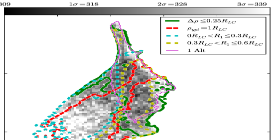
The peaks, $P_{1}$ and $P_{2}$, are separated by $\sim 103^{\circ}$–$134^{\circ}$; thus another possibility is that the emission is not from two magnetic poles but a single broad pulse. Interestingly, with this assumption, models exist within the $1\sigma$ multidimensional contour with $\rho_{\rm{ypt}}=1R_{\rm{LC}}$. Figure 10 shows the $\alpha$–$\zeta$ maps of (unreduced) $\chi^{2}$ for the single broad pulse model. The red contour shows the $3\sigma$ range with the assumption that $\rho_{\rm{ypt}}=1R_{\rm{LC}}$. Additionally, the green contour is the $3\sigma$ contour with a $\Delta\rho\leq 0.25R_{\rm{LC}}$ cut and the thin magenta line is the $3\sigma$ contour if $R_{1}=R_{2}$; these two contours strongly overlap which makes us slightly favor models where $R_{1}\neq R_{2}$. Quite a range of altitudes falls within the $3\sigma$ contours and there is a strong correlation between $R_{1}$ and $\alpha$ and $\zeta$. We also plotted two rough ranges of $R_{1}$ on the $\alpha$–$\zeta$ map to illustrate this correlation. Overall, the polarization position angles associated with $P_{2}$ are very noisy, which translates into noisy $\chi^{2}$ surfaces. To decrease this noise, we applied a $0\fdg 5$ Gaussian smoothing kernel to the map and contours. Additionally, Figure 9, panel (B) shows the polarization sweep derived from a single magnetic pole model with $\alpha=66^{\circ}$ and $\zeta=85^{\circ}$.

For single-pole and double-pole models, fit parameters and errors are reported in Table 5. Overall, adding a finite altitude, whether using a single-pole or two-pole model, significantly decreases the $\chi^{2}_{\rm{min}}$ which can be shown statistically using an $F$-test. The (unreduced) $\chi^{2}_{\rm{min}}=355$ for the RVM and $\rm{DOF}_{1}=2$, and $\rm{DOF}_{2}=203$ for the $F$-test. For the single magnetic pole emission (unreduced $\chi^{2}_{\rm{min}}=309$), the probability of exceeding the resulting $F$ is $P=7.63\times 10^{-7}$; for the two magnetic pole model without an orthogonal mode jump (unreduced $\chi^{2}_{\rm{min}}=311$), the probability of exceeding the resulting $F$ is $P=1.47\times 10^{-6}$; for the two magnetic pole model with an orthogonal mode jump (unreduced $\chi^{2}_{\rm{min}}=314$), the probability of exceeding the resulting $F$ is $P=3.89\times 10^{-6}$.

5.5. J1420$-$6048: Multiple Altitudes and Interstellar Scattering

Figure 11.— In the upper panel, blue points are total radio intensity data, red points are linear polarization intensity data, and green points are circular polarization intensity data for J1420$-$6048. The solid magenta line in the upper panel is the model linear intensity used in fitting. In the bottom panel, blue error bars are polarization position angles used in the fit. The model polarization comes from a fit with (unreduced) $\chi^{2}=435$ (joint fit with data from both 10 cm and 20 cm) and parameters $\alpha=120^{\circ}$, $\zeta=150^{\circ}$, and $R_{1}=0.53R_{\rm{LC}}$ weighted by the model intensity. Panel (A) shows the 10 cm intensity and polarization position angle data and the model with scattering time $\tau\sim 0$ ms. Panel (B) is the 20 cm intensity and polarization position angle data and the model with scattering time $\tau=1.3$ ms. The $\rho_{\rm{ypt}}<1R_{\rm{LC}}$ constraints lie beyond the phase plotted. A phase of zero is the point of closest encounter to the magnetic axis in the model.

Figure 12.— Contours of the joint (unreduced) $\chi^{2}$ set to $3\sigma$ in the $\alpha$–$\zeta$ plane for modeling of the polarization data in 10 cm and 20 cm of J1420$-$6048. Different colors represent fits to different $\tau$, scattering time. Increasing scattering time widens the acceptable fit parameters, decreases the acceptable $\alpha$ values, and decreases $\chi^{2}_{\rm{min}}$.

Figure 13.— Map of the joint (unreduced) $\chi^{2}$ for polarization data in 10 cm and 20 cm of J1420$-$6048 in the $\alpha$–$\zeta$ plane. The model has a scattering constant of $\tau=1.3$ ms. Contours of $3\sigma$ are for three ranges of $R$ to show the correlation between $\alpha$, $\zeta$, and altitude and for $\Delta\rho\leq 0.25R_{\rm{LC}}$ (the most physically inaccurate models) and $\rho_{\rm{ypt}}=1R_{\rm{LC}}$ (the most physically accurate models). Horizontal blue lines indicate the region favored by X-ray torus fitting (Section 5.5.1).

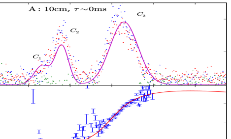
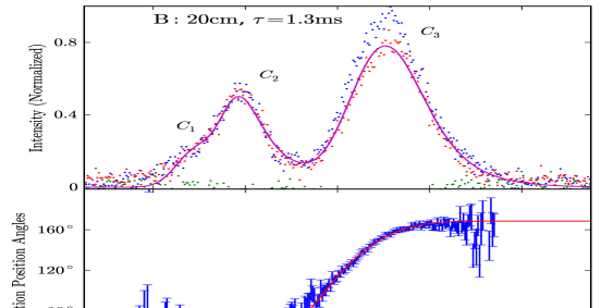
The millisecond pulsar ($P=68$ ms) J1420$-$6048 has been studied previously (Roberts et al. 2001; Weltevrede et al. 2010). The RVM fit in these papers estimated $\alpha>145^{\circ}$ and $\zeta-\alpha\sim 0\fdg 5$ (the angle convention used in these papers is different from that used in this paper and they must be converted. See Everett & Weisberg 2001 for an explanation and the conversion formula). This fit is consistent with our results of fitting with the RVM. Since the effects of interstellar scattering scales to the $-4$ power in frequency (Lang, 1971), comparing 10 cm data to 20 cm data reveals that the polarization and intensity profile of J1420$-$6048 have signs of scattering (Figure 11). In particular, note the widening of the intensity profile and the flattening of the polarization sweep at the trailing edge of the intensity components for the 20 cm data compared to the 10 cm data. The scattering time constant calculated using the Cordes & Lazio (2002) model is $\tau=6.5\times 10^{-2}$ ms. The ratio of $\tau$ to period (and also the value of dispersion measure or DM) is far larger than that for any of the other pulsars considered in this paper yet this value is still smaller than what would cause the scattering seen by comparing the 10 cm and 20 cm data. Because of this discrepancy, $\tau$ is a fit parameter in analyzing polarization data of J1420$-$6048.

When fitting the 10 cm data ($\tau\sim 0$), the best fit non-scattered model is $\alpha=100^{+34(+79)\circ}_{-63(-97)}$, $\zeta=39^{+116(+140)\circ}_{-25(-38)}$, and $R=0.64^{+0.26(+0.26)}_{-0.64(-0.64)}R_{\rm{LC}}$ where errors without (with) parentheses are $1\sigma$ ($3\sigma$) errors. The error bars on these values are large due to the low signal-to-noise in the polarization position angles and the exact parameter values at $\chi^{2}_{\rm{min}}$ are less valuable than the full range defined by these error bars. When fitting the 20 cm polarization data, with a small scattering time ($\tau=0.1$ ms), the best fit non-scattered model is $\alpha=175^{+2(+3)\circ}_{-6(-18)}$, $\zeta=177^{+1(+1)\circ}_{-4(-14)}$, and $R=.37^{+0.10(+0.50)}_{-0.33(-0.37)}R_{\rm{LC}}$ which is drastically different than the results for the 10 cm data. In fact the $3\sigma$ multi-dimensional contours as measured from the individual $\chi^{2}_{\rm{min}}$ do not overlap.

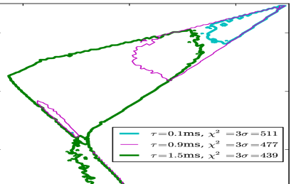
Physically, we expect that two different frequencies should come from different altitudes but we are making the assumption that they are closely spaced and any systematic error from this assumption is overpowered by the statistic error. A combined $\chi^{2}$ from the two sets of data (10 cm and 20 cm) at low scattering constants results in a minimum region similar to the minimum of fitting 20 cm alone (see Figure 12, cyan contours $\tau=0.1$ ms). A combined $\chi^{2}$ from the two sets of data at an intermediate scattering constant results in two distinct minimum regions (see Figure 12, magenta contours $\tau=0.9$ ms). A combined $\chi^{2}$ from the two sets of data at high scattering constants results in a single minimum region (see Figure 12, green contours $\tau=1.5$ ms). In the combined $\chi^{2}$, we assume that the altitudes are the same. Fitting the data with different scattering constants gives drastically different results. The larger the scattering constant, the better the $\chi^{2}_{\rm{min}}$. We can place a practical limit on the scattering because a large scattering constant results in a distorted intensity profile which is not seen in the data. Therefore, we did not fit with a scattering constant larger than $\tau=1.5$ ms since scattering constants much larger than this distort the intensity profile. In Figure 12, as the scattering constant increases, the two islands of best fit $\chi^{2}$ seen at the lowest scattering constant merge into a single $\chi^{2}$ surface. Because of the drastic decrease in $\chi^{2}_{\rm{min}}$ from increasing the scattering constant and the merging of the $\chi^{2}_{\rm{min}}$, the true scattering constant is $\tau\sim 1.1$–$1.5$ ms. Additionally, we report $\alpha$, $\zeta$, and $R$ in Table 6 for select values of $\tau$.

Further, the error bars on the DM are larger than the shift that we expect from including scattering when comparing the two different wavelengths. The DM reported in Weltevrede et al. (2010) is $360^{+2}_{-2}$ cm^-3 pc and the correction to the DM from our fitting of scattering time constants with error bars are reported in Table 6. The $\Delta\rm{DM}$ values are all with in the 2 cm^-3 pc error bars of the original DM up to $3\sigma$ from $\chi^{2}_{\rm{min}}$.

As $\tau$ increases, the best fit values of $\alpha$ and $\zeta$ shift and the $3\sigma$ range for these values increases drastically. Also, the $\chi^{2}_{\rm{min}}$ values decrease statistically significantly from $\tau=0.1$ ms to $\tau=1.5$ ms. For $\tau=1.5$ ms, $3\sigma=439$ from $\chi^{2}_{\rm{min}}$. The $\chi^{2}_{\rm{min}}$ for $\tau=0.1$ ms is not within this $3\sigma$ of the $\tau=1.5$ ms fit.

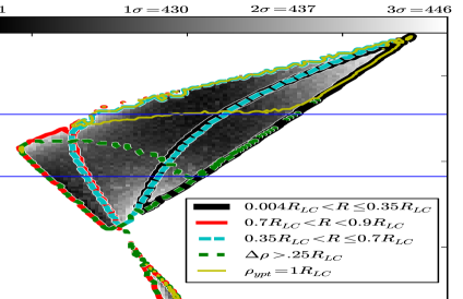
Figure 13 is the (unreduced) $\chi^{2}$ map for $\tau=1.3$ ms. The black, cyan, and red contours are for $3\sigma$ contours at various altitude ranges, illustrating that although the allowed range of altitudes is large for this pulsar, knowledge of $\alpha$ and $\zeta$ could greatly decrease this range because of the correlation between $R$ and $\alpha$–$\zeta$ pairs. A large number of fits could be additionally excluded if cuts of $\Delta\rho$ are applied. The green dashed contour corresponds to $\Delta\rho<0.25R_{\rm{LC}}$. If only fits up to $3\sigma$ with $\rho_{\rm{ypt}}=1R_{\rm{LC}}$ are considered, only fits within the yellow contour on Figure 13 would be allowed.

Table 6Fit Parameters for J1420$-$6048

	$\tau$	(Unreduced)
DOF	(ms)	$\chi^{2}_{\rm{min}}$	$\alpha$ (∘)	$\zeta$ (∘)	$R$ ($R_{\rm{LC}}$)
356-5	.1	$480$	$175^{+3(+4)}_{-15(-77)}$	$177^{+1(+2)}_{-13(-86)}$	$0.37^{+0.10(+0.52)}_{-0.31(-0.37)}$
356-5	.9	$448$	$166^{+13(+13)}_{-76(-81)}$	$169^{+10(+10)}_{-104(-119)}$	$0.26^{+0.64(+0.64)}_{-0.26(-0.26)}$
356-5	1.3	$421$	$126^{+22(+51)}_{-46(-50)}$	$153^{+9(+25)}_{-113(-115)}$	$0.52^{0.38(+0.38)}_{-0.52(-0.52)}$
356-5	1.5	$415$	$105^{+27(+42)}_{-28(-31)}$	$140^{+14(+22)}_{-102(-106)}$	$0.58^{+0.32(+0.32)}_{-0.44(-0.58)}$

5.5.1 X-Ray Torus of J1420$-$6048

Figure 14.— X-ray PWN of PSR J1420$-$6048. Upper left shows the PWN structure, while the figure of merit (FoM) panel show contours of the fit in the $\zeta$–$\beta$ plane. The other panels show the dependence of the torus shape and brightness on these parameters (see Section 5.5.1).

Young pulsars appear to produce relativistic plasma confined to the spin equator. When this wind shocks the $e^{+}/e^{-}$ pitch angle scatter and synchrotron radiate, producing an equatorial torus. Since the bulk flow in the region is mildly relativistic, with expected bulk velocity $\beta\sim 0.3$–$0.7$, this torus can be Doppler brightened on the side emerging from the plane of the sky. In several cases, there seems to be a secondary shock along the polar axis producing polar “jets” in the pulsar wind nebula (PWN), with the jet on the opposite side of the Doppler-enhanced torus rim, being Doppler boosted. The Crab and Vela pulsars provide classic examples of this relativistic torus–jet geometry.

Ng & Romani (2004) and Ng & Romani (2008) showed how fits to Chandra X-ray images of such tori can provide useful constraints on the pulsar spin orientation. For PSR J1420$-$6048, we obtained a 90 ks Chandra ACIS observation (ObSID 12545). We combined this exposure with a 10 ks archival observation (ObsID 2794), removing the spacecraft dither and reprocessing the data giving sub-pixel (EDSER) event positioning, to obtain the best possible image of the compact PWN surrounding this energetic pulsar. Figure  14 (upper left) shows a lightly smoothed 0.7–7 keV Chandara image of the combined exposure, with a logarithmic stretch. The pulsar point source is in the red circle. Unfortunately, this pulsar does not show a striking torus structure, so unlike several other young pulsars, we cannot obtain a high-quality, model-independent measurement of its spin geometry. Still, the diffuse counts do show a semi-circular arc of flux, trailing off to the NE. If we interpret this as an equatorial torus, we can apply the methods of Ng & Romani (2008) to constrain the spin orientation. A few parameters are well measured: the position angle of the symmetry axis ($\Psi=40^{\circ}\pm 3^{\circ}$, measured N through E) and the radius of the “torus” ($7^{\prime\prime}\pm 1\farcs 5$) are reasonably constrained. In unsmoothed images there is some evidence for a polar component on a $1^{\prime\prime}$–$2^{\prime\prime}$ scale, but this is not well measured. The parameter of greatest interest to the present study is the inclination $\zeta$ of the pulsar spin to the Earth line-of-sight. To minimize sensitivity to point source flux and possible jet structure we fit outside of the $5^{\prime\prime}$ radius red circle dominated by the central point source. The main constraint comes from the shape and brightness ratio between the front and back sides of the torus. The second panel of Figure  14 shows that this introduces substantial co-variance between $\zeta$ and the bulk $\beta$ of the post-shock flow. The best fits are near typical $\beta\sim 0.5$, with $\zeta\approx 125^{\circ}$. This is in considerable tension with the larger $\zeta$ preferred by the polarization position angle fits to models with small scattering times; we only reach $\zeta\approx 155^{\circ}$ with a rather aphysical $\beta\sim 0.9$. This co-variance is visible along the bottom row of torus (+PSF+jet) models, which show that as $\zeta$ increases from $130^{\circ}$ to $150^{\circ}$, the post-shock Lorentz factor must grow to maintain a reasonable intensity ratio between the “front” and “back” sides of the torus. The last panel on the top row shows how with $\zeta=150^{\circ}$, $\beta=0.5$, the torus is too face-on and uniform for a good fit to the data. Thus the X-ray PWN structure agrees with the $\gamma$-ray pulse shape, where the observed peak separation $\Delta=0.31$ implies $\zeta\approx 110^{\circ}$–$140^{\circ}$, with the largest $\zeta$ only available in the two-pole caustic picture (Romani & Watters, 2010), which tends to produce too much unpulsed emission.

Polarization position angle fits with scattering constant $\tau=1.3$ ms as discussed in Section 5.5 favor $\zeta$ between $120^{\circ}$ and $150^{\circ}$ as can be seen from the color map of Figure 13. The measurement of $\zeta$ from the X-ray torus fit indicates $\zeta$ between $113^{\circ}$ and $142^{\circ}$ (from the contours of $2\sigma$). The horizontal blue lines on Figure 13 mark the region of $2\sigma$ set by the X-ray torus fitting. By assuming a scattering constant, we not only reconcile the fits of 10 cm and 20 cm data but also find consistency between radio polarization position angle fits and X-ray torus fits.

5.6. J2124$-$3358: A Complex Example

Table 7Fit Parameters for J2124$-$3358

	DOF	(Unreduced) $\chi^{2}_{\rm{min}}$	$\alpha$ (∘)	$\zeta$ (∘)	$R_{1}$ ($R_{\rm{LC}}$)	$R_{2}$ ($R_{\rm{LC}}$)	$R_{3}$ ($R_{\rm{LC}}$)
RVM	536-4	$2331$	$2^{+3(+7)}_{-0(-0)}$	$5^{+8(+19)}_{-0(-0)}$	$\cdots$	$\cdots$	$\cdots$
3 Alt	536-7	$773$	$2^{+7(+12)}_{-1(-1)}$	$2^{+7(+12)}_{-1(-1)}$	$0.05^{+0.01(+0.03)}_{-0.00(-0.00)}$	$0.40^{+0.01(+0.02)}_{-0.01(-0.03)}$	$0.55^{+0.02(+0.04)}_{-0.01(-0.03)}$

Figure 15.— In the upper panel, blue points are total radio intensity data for 1.369 GHz, red points are linear polarization intensity data, and green points are circular polarization intensity data for J2124$-$3358. The solid magenta line in the upper panel is the model linear intensity used in fitting. In the bottom panel, blue error bars are polarization position angles used in the fit and yellow error bars are polarization position angles excluded by error bar cuts. The model polarization comes from a fit with (unreduced) $\chi^{2}=773$ and parameters $\alpha=2^{\circ}$ and $\zeta=2^{\circ}$. The green solid line is the polarization for a model with $R_{1}=0.05R_{\rm{LC}}$ (associated with intensity components $C_{1}$ and $C_{2}$), the black solid line is the polarization for a model with $R_{2}=0.40R_{\rm{LC}}$ (associated with intensity components $C_{3}$, $C_{4}$, and $C_{5}$), and the cyan solid line is the polarization for a model with $R_{2}=0.55R_{\rm{LC}}$ (associated with intensity components $C_{6}$, $C_{7}$, and $C_{8}$). We assumed that the polarization associated with components $C_{1}$, $C_{2}$, and $C_{6}$ are orthogonal to the polarization associated with components $C_{3}$, $C_{4}$, $C_{5}$, $C_{7}$, and $C_{8}$. The red solid line is the model polarization of the three altitudes weighted by the model intensity. There are clearly features in the data that are not captured by the model but the overall structure of the polarization is captured. A phase of zero is the point of closest encounter to the magnetic axis in the model.

Figure 16.— Map of (unreduced) $\chi^{2}$ for J2124$-$3358 in the $\alpha$–$\zeta$ plane. All of the fitted models within $3\sigma$ from $\chi^{2}_{\rm{min}}$ have a phase of emission that is within the phase of emission predicted by the models and thus $\rho_{\rm{ypt}}=1R_{\rm{LC}}$ is acceptable.

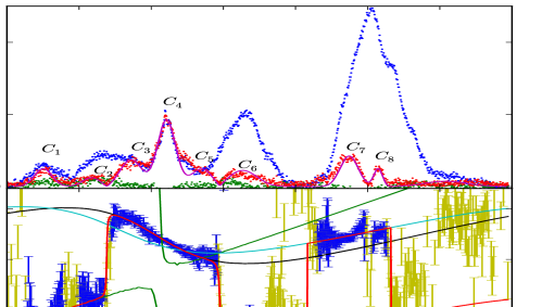
J2124$-$3358 is yet another millisecond pulsar ($P=4.931$ ms). Plotted in Figure 15 is the polarization and intensity profile for this pulsar at 1.369 GHz. The pulsar J2124$-$3358 has emission at practically all phases of the period. The polarization position angles are complicated but can be greatly simplified by assuming orthogonal mode jumps at the appropriate components. We assumed that the polarization associated with components $C_{1}$, $C_{2}$, and $C_{6}$ are orthogonal to the polarization associated with components $C_{3}$, $C_{4}$, $C_{5}$, $C_{7}$, and $C_{8}$ as labeled in Figure 15. With these orthogonal mode jumps, the polarization forms a close-to-continuous sweep and the RVM can be reasonably fit to the data. Table 7 reports the best fit values and (unreduced) $\chi^{2}_{\rm{min}}$ for this fit.

With the assumption of multiple altitudes and mode jumps, the polarization was also fit. More than three altitudes did not significantly improve the fit. Also plotted in Figure 15 (top panel) is the best fit polarization model with multiple altitudes. The polarization associated with components $C_{1}$ and $C_{2}$ is assigned one altitude ($R_{1}$); the polarization associated with components $C_{3}$, $C_{4}$, and $C_{5}$ is assigned the second altitude ($R_{2}$); and the polarization associated with components $C_{6}$, $C_{7}$, and $C_{8}$ is assigned the third altitude ($R_{3}$). The fit is far from perfect and does not capture the many bumps and wiggles in the polarization data. The model does capture the overall curvature of the polarization and significantly decreases the $\chi^{2}$ (Table 7) although the $\alpha$ and $\zeta$ values do not change drastically between the two fits. For the RVM (unreduced) $\chi^{2}_{\rm{min}}=2331$ and for the three-altitude model (unreduced) $\chi^{2}_{\rm{min}}=773$. The $F$-test between RVM and the two-altitude model gives $F=355.4$, $\rm{DOF}_{1}=3$, and $\rm{DOF}_{2}=529$. The probability of exceeding this $F$ is $\rm{Prob}\sim 0$, indicating the addition of altitude to the model is highly statistically significant.

The curvature direction of the bridging polarization sweep between orthogonal mode jumps is important here similar to the polarization of J0023$+$0923 in Section 5.1. As discussed in Section 3.3, for a single-altitude polarization sweep with an orthogonal mode jump, the bridging section of polarization between the two modes will have the opposite curvature of that of the original sweep due to forward scattering. In J2124$-$3358 between the polarization components associated with the intensity components $C_{5}$ and $C_{6}$, the bridging sweep direction has a negative curvature and the original sweep direction is also negative. This indicates that the polarization of these two components are not exactly $90^{\circ}$, which is consistent with a multi-altitude model that has non-$90^{\circ}$ orthogonal jumps between altitudes.

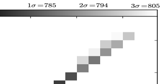
The values for $R_{1}$, $R_{2}$, and $R_{3}$ are quite restrictive and the statistical error bars on these values are quite small. These values are small because very few altitude combinations capture the subtle difference between polarization associated with the various components; for instance, note the rather large offset between the black and cyan solid lines in Figure 15 which represent model polarization from $R_{1}$ and $R_{2}$. Only very particular sets of altitude will result in polarization with this amount of vertical shift. Also, $\rho_{\rm{ypt}}=1R_{\rm{LC}}$ for all fits within the $3\sigma$ bound of $\chi^{2}_{\rm{min}}$ due to the small geometrical angles ($\alpha$ and $\zeta$, see Figure 16).

6. Conclusion

In this paper, we attempted to push the limit of what we can learn from geometrical-based models applied to radio polarization. We have shown that this model can explain polarization for which the RVM fails (partially or fully) and can significantly alter fit parameters ($\alpha$ and $\zeta$) obtained from the RVM. We have shown that a handful of physical effects can alter our understanding of the geometry of millisecond and young pulsar radio emission. Additionally, we provided statistical comparisons to simpler models to quantify the significance of adding these physical phenomena to the model.

Both J0023$+$0923 and J1024$-$0719 clearly illustrate how multi-altitudes can capture the non-$90^{\circ}$ jumps seen in the position angle sweeps of the millisecond pulsar population. J1057$-$5226 and J1744$-$1134 illustrate the need for finite altitude and $\rho_{\rm{ypt}}<R_{\rm{LC}}$ to fully explain the large phase range of the emission seen in the data. J1420$-$6048 illustrates how scattering affects can rectify discrepancies seen between multi-wavelength data. Finally, J2124$-$3358 is a typical worst-case radio polarization from a millisecond pulsar. Despite its clear non-RVM characteristics, we were able to capture the overall structure of the polarization position angles sweep with finite and multiple altitudes and orthogonal mode jumps.

The RVM is not accurate for the radio polarization sweeps of these energetic pulsars. First, this emission originated from a significant fraction of the light cylinder which necessitates numerical calculation of this radio polarization. Additionally, non-$90^{\circ}$ jumps cannot be explained by simple orthogonal mode jumps and some polarization is scattered by the interstellar medium. Polarization of millisecond pulsars is notoriously hard to model and very few studies have attempted to tackle these objects. That we can explain some of the polarization of these pulsars is a significant step in the correct direction. This is a methods paper; with various example polarization data from a number of pulsars, we have shown that this method of using physically motivated, geometrically based phenomena can explain the inconsistencies of simpler models.

References

- Backer et al. (1976) Backer, D., Rankin, J. M., & Campbell, D. 1976, Nature, 263, 202
- Blaskiewicz et al. (1991) Blaskiewicz, M., Cordes, J., & Wasserman, I. 1991, The Astrophysical Journal, 370, 643
- Cordes & Lazio (2002) Cordes, J. M., & Lazio, T. J. W. 2002, arXiv preprint astro-ph/0207156
- Craig & Romani (2012) Craig, H., & Romani, R. W. 2012, The Astrophysical Journal, 755, 137
- Cronyn (1970) Cronyn, W. M. 1970, The Astrophysical Journal, 161, 755
- Dyks (2008) Dyks, J. 2008, Monthly Notices of the Royal Astronomical Society, 391, 859
- Everett & Weisberg (2001) Everett, J., & Weisberg, J. 2001, The Astrophysical Journal, 553, 341
- Flannery et al. (1992) Flannery, B. P., Press, W. H., Teukolsky, S. A., & Vetterling, W. 1992, Press Syndicate of the University of Cambridge, New York
- Gould & Lyne (1998) Gould, D., & Lyne, A. 1998, Monthly Notices of the Royal Astronomical Society, 301, 235
- Kaburaki (1980) Kaburaki, O. 1980, Astrophysics and Space Science, 67, 3
- Kalapotharakos et al. (2012) Kalapotharakos, C., Harding, A. K., Kazanas, D., & Contopoulos, I. 2012, The Astrophysical Journal Letters, 754, L1
- Karastergiou (2009) Karastergiou, A. 2009, Monthly Notices of the Royal Astronomical Society: Letters, 392, L60
- Karastergiou & Johnston (2007) Karastergiou, A., & Johnston, S. 2007, Monthly Notices of the Royal Astronomical Society, 380, 1678
- Karastergiou et al. (2005) Karastergiou, A., Johnston, S., & Manchester, R. 2005, Monthly Notices of the Royal Astronomical Society, 359, 481
- Lang (1971) Lang, K. 1971, Astrophysical Letters, 7, 175
- Li & Han (2003) Li, X., & Han, J. 2003, arXiv preprint astro-ph/0308095
- Lyne & Manchester (1988) Lyne, A., & Manchester, R. 1988, Monthly Notices of the Royal Astronomical Society, 234, 477
- Ng & Romani (2004) Ng, C.-Y., & Romani, R. W. 2004, The Astrophysical Journal, 601, 479
- Ng & Romani (2008) —. 2008, The Astrophysical Journal, 673, 411
- Phillips (1990) Phillips, J. 1990, The Astrophysical Journal, 361, L57
- Radhakrishnan & Cooke (1969) Radhakrishnan, V., & Cooke, D. 1969, Astrophysical Letters, 3, 225
- Roberts et al. (2001) Roberts, M. S., Romani, R. W., & Johnston, S. 2001, The Astrophysical Journal Letters, 561, L187
- Romani & Watters (2010) Romani, R. W., & Watters, K. P. 2010, The Astrophysical Journal, 714, 810
- Spitkovsky (2006) Spitkovsky, A. 2006, The Astrophysical Journal Letters, 648, L51
- Stinebring et al. (1984) Stinebring, D., Cordes, J., Rankin, J., Weisberg, J., & Boriakoff, V. 1984, The Astrophysical Journal Supplement Series, 55, 247
- Watters & Romani (2011) Watters, K. P., & Romani, R. W. 2011, Astrophys.J., 727, 123
- Weltevrede & Wright (2009) Weltevrede, P., & Wright, G. 2009, Monthly Notices of the Royal Astronomical Society, 395, 2117
- Weltevrede et al. (2010) Weltevrede, P., Abdo, A. A., Ackermann, M., et al. 2010, The Astrophysical Journal, 708, 1426
- Yan et al. (2011) Yan, W., Manchester, R., van Straten, W., et al. 2011, Monthly Notices of the Royal Astronomical Society, 414, 2087