New ways to search for right-handed current in $B\to\rho\ell\bar{\nu}$ decay

Abstract

An interesting possibility to ease the tension between various determinations of $|V_{ub}|$ is to allow a small right-handed contribution to the standard model weak current. The present bounds on such a contribution are fairly weak. We propose new ways to search for such a beyond standard model contribution in semileptonic $B\to\rho\ell\bar{\nu}$ decay. Generalized asymmetries in one, two, or three angular variables are introduced as discriminators, which do not require an unbinned analysis of the fully differential distribution, and a detailed study of the corresponding theoretical uncertainties is performed. A discussion on how binned measurements can access all the angular information follows, which may be useful in both $B\to\rho\ell\bar{\nu}$ and $B\to K^{*}\ell^{+}\ell^{-}$, and possibly essential in the former decay due to backgrounds. The achievable sensitivity from the available ${\displaystyle B}\!{\scriptstyle A}{\displaystyle B}\!{\scriptstyle AR}$ and Belle data sets is explored, as well as from the anticipated $50\,{\rm ab}^{-1}$ Belle II data.

I Introduction

There is a long standing persistent tension between measurements of $|V_{ub}|$ from $B$ decays in leptonic, inclusive semileptonic, and exclusive semileptonic decay channels. In semileptonic decays, the difference between the inclusive determination and that based on $B\to\pi\,\ell\bar{\nu}$ is almost 3$\sigma$. It is possible that the resolution of this is related to not sufficiently understood theoretical or experimental issues, and future theory progress combined with the anticipated much larger Belle II data sets will yield better consistency. A precise determination of $|V_{ub}|$ is crucial for improving tests of the standard model (SM) and the sensitivity to new physics in $B^{0}-\,\overline{\!B}{}{}^{0}$ mixing Charles:2013aka .

Another possibility, which received renewed attention recently Crivellin:2009sd ; Buras:2010pz , is that this tension can be eased by allowing for a right-handed admixture to the SM weak current. Such a contribution could arise from not yet discovered TeV-scale new physics. In general, from a low energy effective theory point of view, the SM can be extended by several new operators relevant for semileptonic decays, suppressed by ${\cal O}(v^{2}/\Lambda^{2})$ Feger:2010qc ; Faller:2011nj , where $\Lambda$ is a high scale related to new physics. For simplicity, we consider the effective Lagrangian with only one new parameter,

$$\mathcal{L}_{\text{eff}}=-\frac{4G_{F}}{\sqrt{2}}V_{ub}^{L}\big{(}\bar{u}\gamma_{\mu}P_{L}b+\epsilon_{R}\,\bar{u}\gamma_{\mu}P_{R}b\big{)}(\bar{\nu}\gamma^{\mu}P_{L}\ell)+\text{h.c.},$$ (1)

where $P_{L,R}=(1\mp\gamma_{5})/2$. The SM is recovered as $\epsilon_{R}\to 0$. Since we consider observables with leading, linear, dependence on Re $(\epsilon_{R})$, we assume it to be real in this paper, unless indicated otherwise. This happens to be the expectation in models with flavor structures close to minimal flavor violation. We do not consider $b\to c\ell\nu$ decay in this paper, as the tension between the determinations of $|V_{cb}|$ is less severe, and the connection between $b\to u$ and $b\to c$ transitions is model dependent (see, however, Ref. Crivellin:2014zpa ). To distinguish from determinations of $|V_{ub}|$ assuming the SM, we refer to analyses which allow for $\epsilon_{R}\neq 0$ as measurements of $|V_{ub}^{L}|$.

Decay	$\left|V_{ub}\right|\times 10^{3}$	$\epsilon_{R}$ dependence
$B\to\pi\,\ell\bar{\nu}$	$3.23\pm 0.30$	$1+\epsilon_{R}$
$B\to X_{u}\ell\bar{\nu}$	$4.39\pm 0.21$	$\sqrt{1+\epsilon_{R}^{2}}$
$B\to\tau\,\bar{\nu}_{\tau}$	$4.32\pm 0.42$	$1-\epsilon_{R}$
Decay	${\cal B}\times 10^{4}$
$B\to\rho\,\ell\bar{\nu}$	$1.97\pm 0.16$ ($q^{2}<12$ GeV2)
$B\to\omega\,\ell\bar{\nu}$	$0.61\pm 0.11$ ($q^{2}<12$ GeV2)

Table 1: The $|V_{ub}|$ measurements Amhis:2012bh used in the fit shown in Fig. 1 and their dependence on $\epsilon_{R}$. The branching fractions are taken from Ref. Sibidanov:2013rkk

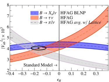
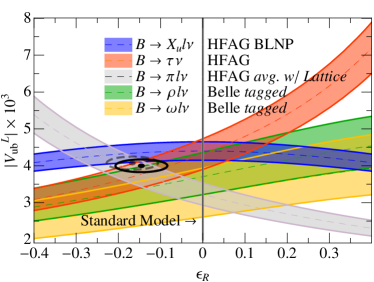
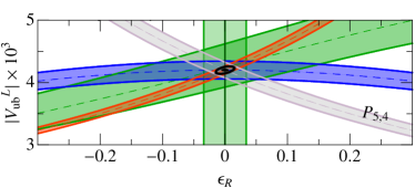
The current measurements of $|V_{ub}|$ are summarized in Table 1, and their dependence on $\epsilon_{R}$ is indicated in the three cases in which it is simple. The $\rho$ and $\omega$ measurements are from Ref. Sibidanov:2013rkk using the theoretical predictions of Ref. Ball:2004rg , and the two isospin-related $\rho$ modes were averaged assuming a 35% correlation of the systematic uncertainties Sibidanov:2013rkk . While we do not study the $\omega$ final state, it could provide complementary information in the future if lattice QCD calculations of the form factors become available. For $B\to X_{u}\ell\bar{\nu}$ the BLNP result was used. The result of the $\chi^{2}$ fit for $|V_{ub}^{L}|-\epsilon_{R}$ without and with $B\to\rho\,\ell\bar{\nu}$ are shown in Fig. 1.

Figure 1: The allowed $|V_{ub}^{L}|-\epsilon_{R}$ regions. The black ellipse in the left (right) plot shows the result of a $\chi^{2}$ fit using the first three (four, excluding $\omega$) measurements in Table 1. The fainter ellipse in the right plot is the same as that in the left plot.

The goal of this this paper is to devise observables sensitive to new physics contributions in $\epsilon_{R}$, without requiring the measurement of the fully differential decay distribution. It is well-known from the literature on both semileptonic and rare decays that a full description of the four-body final state in $B\to\rho\ell\bar{\nu}$ depends on the dilepton invariant mass, $q^{2}$, and three angles. While we assume that the neutrino four-momentum is reconstructed, past studies of $B\to D^{*}$ Aubert:2007rs ; Dungel:2010uk and $D\to\rho$ CLEO:2011ab semileptonic decays show that for $B\to\rho\ell\bar{\nu}$, which has a much smaller rate, the full angular analysis will be challenging and may be many years in the future. Thus, it is interesting to explore how the best sensitivity to $\epsilon_{R}$ may be obtained using current and near future data sets.

Fit	$|V_{ub}^{L}|\times 10^{4}$	$\epsilon_{R}$	$\chi^{2}$ / ndf	Prob.
3 modes	$4.07\pm 0.18$	$-0.17\pm 0.06$	2.5 /1	0.11
4 modes	$4.00\pm 0.17$	$-0.15\pm 0.06$	4.5 /2	0.11

Table 2: The results of the $\chi^{2}$ fits to the first 3 and all modes but $\omega$ in Table 1. The correlation between $|V_{ub}^{L}|$ and $\epsilon_{R}$ in the two fits are 0.01 and 0.01.

In Section II we discuss the decay rate distributions. Besides investigating the well known forward-backward asymmetry, we propose a generalized two-dimensional asymmetry as a new observable that would be interesting to measure. Additionally we explore the possibility to extract the full information on the differential rate by considering asymmetries in all three angles simultaneously. In Section III we discuss the theoretical uncertainties in existing form factor calculations. Using results from a light-cone sum rule calculation Ball:2004rg , we estimate the correlations among the uncertainties. Then we perform a simultaneous fit to a (simplified) series expansion parametrization of the form factors. In Section IV we discuss the best theoretical predictions to extract information on right-handed currents. We investigate the discriminating contour for the two dimensional asymmetry. We estimate the sensitivity both with the current $B$-factory data, as well as with the anticipated Belle II dataset to compare the various observables. We use this information in Section V to explore the impact of the sensitivity to right-handed currents by performing global fits simultaneously to $|V_{ub}^{L}|$ and $\epsilon_{R}$ assuming different scenarios for both the current $B$-factory as well as expected Belle II dataset. Section VI contains our conclusions.

II Possible observables

Starting from the Lagrangian in Eq. (1), the $B\to\rho\ell\bar{\nu}$ decay is described by replacing in the matrix element the vector ($V$) and the three axial-vector ($A_{0,1,2}$) form factors via

$$V\to(1+\epsilon_{R})\,V\,,\qquad A_{i}\to(1-\epsilon_{R})\,A_{i}\,.$$ (2)

(If ${\rm Im}\,\epsilon_{R}=0$ then this can be done in the decay rate, too.) Recently, the similar $B\to K^{*}\ell^{+}\ell^{-}$ decay has received a lot of attention, in which case the decay distributions are in exact analogy with $B\to\rho\ell\bar{\nu}$ (assuming that the neutrino is reconstructed). It has been advocated Matias:2012xw to use the form factor relations proposed in the heavy quark limit Charles:1998dr ; Burdman:1998mk to construct observables, which are ratios of terms in the fully differential decay distribution, to optimize sensitivity to new physics. However, the size of perturbative and nonperturbative corrections to these relations are subject to discussions Bauer:2002aj ; Beneke:2002ph ; Jager:2012uw . Thus, other recent papers Hambrock:2013zya also have to resort to some extent to QCD sum rule calculations to estimate the corrections to the form factor relations, which we discuss in Sec. III.

II.1 The general parameterization

The fully differential decay rate for the four-body decay $B\to\rho(\to\pi\pi)\ell^{-}\bar{\nu}_{\ell}$ can be written in terms of four variables. These are conventionally chosen as the momentum transfer to the dilepton system, $q^{2}$, and three angles describing the relative orientation of the final state particles. As usual, we choose $\theta_{V}$ as the angle of the $\pi^{+}$ in the $\rho$ restframe with respect to the $\rho$ direction in the $B$ restframe. Similarly, $\theta_{\ell}$ is the angle of the $\ell^{-}$ in the dilepton restframe with respect to the direction of the virtual $W^{-}$ in the $B$ restframe. Finally $\chi$ is the angle between the decay planes of the hadronic and leptonic systems in the $B$ restframe. This convention coincides with the usual definition in the similar flavor-changing neutral-current decay $B\to K^{*}(\to K\pi)\ell^{+}\ell^{-}$ Jager:2012uw ; Descotes-Genon:2013vna . The fully differential rate is

$$\frac{\text{d}\Gamma}{\text{d}q^{2}\,\text{d}\cos\theta_{V}\,\text{d}\cos\theta_{\ell}\,\text{d}\chi}=\frac{G_{F}^{2}|V_{ub}^{L}|^{2}m_{B}^{3}}{2\pi^{4}}$$

$$\times\bigg{\{}J_{1s}\sin^{2}\theta_{V}+J_{1c}\cos^{2}\theta_{V}$$

$$+(J_{2s}\sin^{2}\theta_{V}+J_{2c}\cos^{2}\theta_{V})\cos 2\theta_{\ell}$$

$$+J_{3}\sin^{2}\theta_{V}\sin^{2}\theta_{\ell}\,\cos 2\chi$$

$$+J_{4}\sin 2\theta_{V}\sin 2\theta_{\ell}\,\cos\chi+J_{5}\sin 2\theta_{V}\sin\theta_{\ell}\,\cos\chi$$

$$+(J_{6s}\sin^{2}\theta_{V}+J_{6c}\cos^{2}\theta_{V})\cos\theta_{\ell}$$

$$+J_{7}\sin 2\theta_{V}\sin\theta_{\ell}\,\sin\chi+J_{8}\sin 2\theta_{V}\sin 2\theta_{\ell}\,\sin\chi$$

$$+J_{9}\sin^{2}\theta_{V}\sin^{2}\theta_{\ell}\,\sin 2\chi\bigg{\}}\,.$$ (3)

Our convention for the ranges of the angular variables are $\chi\in[0,2\pi]$, $\theta_{\ell}\in[0,\pi]$, $\theta_{V}\in[0,\pi]$. Switching $\chi\to\chi-\pi$, so that $\chi\in[-\pi,\pi]$, customary in $B\rightarrow K^{*}\ell^{+}\ell^{-}$, amounts to a sign flip in the terms

$$\{J_{4},\,J_{5},\,J_{7},\,J_{8}\}\to\{-J_{4},\,-J_{5},\,-J_{7},\,-J_{8}\}\,.$$ (4)

The dependence on $q^{2}$, as well as that on all form factors and on the NP parameter $\epsilon_{R}$, is contained in the 12 dimensionless $J_{i}(q^{2},\epsilon_{R})$ functions. For the Lagrangian in Eq. (1), some simplifications occur

$$J_{1s}=3J_{2s}\,,\qquad J_{1c}=-J_{2c}\,,\qquad J_{7}=0\,,$$ (5)

and additionally $J_{6c}=0$ for massless leptons. While the functions $J_{7,8,9}$ are proportional to $\text{Im}\,\epsilon_{R}$, the other $J_{i}$ functions start with $(\text{Im}\,\epsilon_{R})^{2}$ and $\text{Re}\,\epsilon_{R}$, and so they are mainly sensitive to $\text{Re}\,\epsilon_{R}$. Partially integrated rates can be found in Appendix A.

An important difference between $B\to\rho\ell\bar{\nu}$ and $B\to K^{*}\ell^{+}\ell^{-}$ is that in the former case the leptonic current is constrained to be left-handed, and in the latter case several operators contribute already in the SM, thus it is more compelling to study all possible NP contributions. (Right-handed $\ell\bar{\nu}$ couplings are severely constrained, e.g., by Michel parameter analyses.) The rate corresponding to switching from left-handed to right-handed leptonic current is obtained by the replacement $\theta_{\ell}\to\theta_{\ell}-\pi$, resulting in a sign flip of the terms

$$\{J_{5},\,J_{6s},\,J_{6c},\,J_{7}\}\to\{-J_{5},\,-J_{6s},\,-J_{6c},\,-J_{7}\}\,.$$ (6)

(As well as multiplication by the square of the right-handed coupling; neglecting lepton masses, there is no interference between the two lepton couplings.) This difference can only be seen in an angular analysis, as it does not contribute after integration over the angles. The $q^{2}$ spectrum depends on $2J_{1s}+J_{1c}-(2J_{2s}+J_{2c})/3$ and hence is insensitive to the chirality of the lepton current.

In $B\to K^{*}\ell^{+}\ell^{-}$ decay, a set of “clean observables” were proposed Matias:2012xw , which can be calculated model independently in the SM, if the so-called “non-factorizable” contributions dominate the form factors Bauer:2002aj . These observables are ratios of the $J_{i}$ functions, constructed so that these non-factorizable contributions cancel at each value of $q^{2}$, while there are corrections from power suppressed effects as well as calculable “factorizable” contributions. The cancellation of the non-factorizable contributions arises because in the heavy $b$-quark limit, the number of independent nonperturbative parameters is reduced due to the symmetries of SCET Bauer:2000ew ; Bauer:2001yt . However, even in this case, symmetry breaking corrections may be a significant limitation in practice Jager:2012uw . In the following we explore the possibilities of constructing observables sensitive to a right-handed current.

A fully differential analysis in four-dimensions, as required for the determination of the $J_{i}$ in bins of $q^{2}$ for the calculation of the “clean observables” is experimentally challenging: an unbinned fit to the four-dimensional decay rates requires parametrizing the background components and their correlations adequately and when faced with this problem experimentalists often choose alternative approaches, e.g., projections are analyzed (see Refs. Aubert:2007rs ; Dungel:2010uk ) or event probabilities are assigned (see, e.g., Ref. CLEO:2011ab ). Both methods are complicated, and as we are interested in the search for right-handed currents, corresponding to constraining a single unknown parameter, we explore simpler variables, which amount to counting experiments in different regions of phase space.

II.2 One- and generalized two-dimensional asymmetries

It is well known that the forward-backward asymmetry is sensitive to the chiral structure of currents contributing to a decay,

$$A_{\rm FB}=\frac{\int_{-1}^{0}\text{d}\cos\theta_{\ell}(\text{d}\Gamma/\text{d}\cos\theta_{\ell})-\int_{0}^{1}\text{d}\cos\theta_{\ell}(\text{d}\Gamma/\text{d}\cos\theta_{\ell})}{\int_{-1}^{1}\text{d}\cos\theta_{\ell}\,(\text{d}\Gamma/\text{d}\cos\theta_{\ell})}\,.$$ (7)

We study the sensitivity of this variable to $\epsilon_{R}$ in Sec. IV, after discussing the form factor inputs used. The one-dimensional distributions in $\chi$ and $\theta_{V}$ are symmetric, and hence it is not possible to construct asymmetry-type observables with good sensitivity to $\epsilon_{R}$ from these one-dimensional distributions.

Next, we integrate over one of the three angles, which reduces the number of contributing $J_{i}$. We achieve the best sensitivity by integrating over the angle $\chi$, which leaves us with

$$\frac{\text{d}\Gamma}{\text{d}q^{2}\,\text{d}\cos\theta_{V}\,\text{d}\cos\theta_{\ell}}=\frac{G_{F}^{2}\,|V_{ub}^{L}|^{2}\,m_{B}^{3}}{\pi^{3}}\,\bigg{\{}J_{1s}\sin^{2}\theta_{V}$$

$$+J_{1c}\cos^{2}\theta_{V}+(J_{2s}\sin^{2}\theta_{V}+J_{2c}\cos^{2}\theta_{V})\cos 2\theta_{\ell}$$

$$+(J_{6s}\sin^{2}\theta_{V}+J_{6c}\cos^{2}\theta_{V})\cos\theta_{\ell}\bigg{\}}\,$$ (8)

and $J_{6c}=0$ for massless leptons. This limits the possible observables substantially, and none of the “clean observables” sensitive to $\epsilon_{R}$ are accessible from measurement of this triple differential rate only.

To optimize the sensitivity from this class of measurements, we introduce new observables,

$$S=\frac{A-B}{A+B}\,,$$ (9)

where $A$ and $B$ are the decay rates in two regions in the $\{\cos\theta_{\ell},\,\cos\theta_{V}\}$ parameter space, chosen such that $S\simeq 0$ in the SM. This is a generalization of the forward-backward asymmetry, which may have increased sensitivity to $\epsilon_{R}$. To improve the statistical precision, we integrate over a suitably chosen interval of $q^{2}$. Given the available constraints on the form factors, we integrate over $0\leq q^{2}\leq 12\,\text{GeV}^{2}$ to balance between experimental and theoretical uncertainties.

$J_{i}$	$\eta_{i}^{\chi}$	$\eta_{i}^{\theta_{\ell}}$	$\eta_{i}^{\theta_{V}}$	normalization $N_{i}$
$J_{1s}$	$\{+\}$	$\{+,a,a,+\}$	$\{-,c,c,-\}$	$2\pi(1)2$
$J_{1c}$	$\{+\}$	$\{+,a,a,+\}$	$\{+,d,d,+\}$	$2\pi(1)(2/5)$
$J_{2s}$	$\{+\}$	$\{-,b,b,-\}$	$\{-,c,c,-\}$	$2\pi(-2/3)2$
$J_{2c}$	$\{+\}$	$\{-,b,b,-\}$	$\{+,d,d,+\}$	$2\pi(-2/3)(2/5)$
$J_{3}$	$\{+,-,-,+,+,-,-,+\}$	$\{+\}$	$\{+\}$	$4(4/3)^{2}$
$J_{4}$	$\{+,+,-,-,-,-,+,+\}$	$\{+,+,-,-\}$	$\{+,+,-,-\}$	$4(4/3)^{2}$
$J_{5}$	$\{+,+,-,-,-,-,+,+\}$	$\{+\}$	$\{+,+,-,-\}$	$4(\pi/2)(4/3)$
$J_{6s}$	$\{+\}$	$\{+,+,-,-\}$	$\{-,c,c,-\}$	$2\pi(1)2$
$J_{6c}$	$\{+\}$	$\{+,+,-,-\}$	$\{+,d,d,+\}$	$2\pi(1)(2/5)$
$J_{7}$	$\{+,+,+,+,-,-,-,-\}$	$\{+\}$	$\{+,+,-,-\}$	$4(\pi/2)(4/3)$
$J_{8}$	$\{+,+,+,+,-,-,-,-\}$	$\{+,+,-,-\}$	$\{+,+,-,-\}$	$4(4/3)^{2}$
$J_{9}$	$\{+,+,-,-,+,+,-,-\}$	$\{+\}$	$\{+\}$	$4(4/3)^{2}$

Table 3: Definition of the asymmetries in the three angles in bin-size of $\pi/4$, see Eq- (10). The $\pm$ signs denote $\pm 1$, and $\{+\}$ denotes $+1$ in all entries in a given column. Simple choices are $a=1-1/\sqrt{2}$, $b=a\sqrt{2}$, $c=2\sqrt{2}-1$, and $d=1-4\sqrt{2}/5$.

It is important to estimate a reliable theoretical uncertainty for the asymmetry $S$. A priori, one may think that the hadronic uncertainties in the numerator and the denominator cancel in the ratio to a large extent. As it is shown below, we cannot simply assume such a cancellation of nonperturbative uncertainties in the ratios of the binned rates, as the considered $q^{2}$ region is sizable. We develop a model for the uncertainties and correlations among the binned rates, using available calculations of the form factors. The optimal separation which discriminates between the two regions, $A$ and $B$, depends on this choice of the $q^{2}$ range. Thus it is crucial to test the sensitivity of the result to nonperturbative uncertainties.

II.3 Binned measurements of the $J_{i}$ coefficients

The previous approaches have the limitations of not allowing to chose the numerator and denominator arbitrarily in terms of the $J_{i}$ functions. The extraction of the full set of these coefficients is experimentally challenging, and we propose a method that may allow for a better extraction of these coefficients. (The determination of a subset of the $J_{i}$ coefficients from binned rates was explored in Ref. DeCian .) We then investigate the sensitivity of arbitrary ratios of the $J_{i}$.

The form of the differential rate in Eq. (II.1) enables us to separate each coefficient function $J_{i}$ from binning the three angles in fairly large, $\pi/2$ size, bins. Since some bin-boundaries need to be at half-integer multiples of $\pi/2$, we use a notation where $\chi$ and $\theta_{V,\ell}$ are split into 8 and 4 equal bins of size $\pi/4$, respectively. We can then write

$$J_{i}=\frac{1}{N_{i}}\,\sum_{j=1}^{8}\,\sum_{k,l=1}^{4}\eta_{i,j}^{\chi}\,\eta_{i,k}^{\theta_{\ell}}\,\eta_{i,l}^{\theta_{V}}\Big{[}\chi^{(j)}\otimes\theta_{\ell}^{(j)}\otimes\theta_{V}^{(k)}\Big{]}\,,$$ (10)

where the $\eta^{\alpha}_{i,n}$ are weight factors listed in Table 3, and the term in square brackets denotes the partial rate in the bin labeled by $jkl$. Thus, one can obtain the coefficient functions $J_{i}$ at each value of $q^{2}$, or in bins of $q^{2}$, $\bar{J}_{i}=\int_{\Delta q^{2}}\text{d}q^{2}J_{i}$. Taking ratios of $J_{i}$-s to cancel some experimental and theoretical uncertainties, as well as the dependence on $|V_{ub}|$, leads to observables closely related to the $P_{i}$ “clean observables” in the literature.

Here a somewhat different way of extracting all the $J_{i}$ is proposed. For $B\to K^{*}\ell^{+}\ell^{-}$ the angular folding technique was used Aaij:2013iag to extract these observables either via a counting method or via a full unbinned fit. An unbinned analysis is more difficult for $B\to\rho\ell\bar{\nu}$ due to the sizable $B\to X_{u}\ell\bar{\nu}$ background. This background cannot be assumed to be completely uncorrelated in the three-angle differential distribution, which complicates the parametrization of the background considerably. Extracting all $J_{i}$-s from a binned asymmetry enables one to perform cross-checks with the angular folding technique for all observables DeCian , also in the case of $B\to K^{*}\ell^{+}\ell^{-}$.

In analogy with Ref. Descotes-Genon:2013vna , we define

$$\langle P_{1}\rangle_{\text{bin}} =\frac{1}{2}\frac{\int_{\Delta q^{2}}\text{d}q^{2}J_{3}}{\int_{\Delta q^{2}}\text{d}q^{2}J_{2s}}\,,$$ (11)

$$\langle P_{4}^{\prime}\rangle_{\text{bin}} =\frac{\int_{\Delta q^{2}}\text{d}q^{2}J_{4}}{\sqrt{-\int_{\Delta q^{2}}\text{d}q^{2}J_{2s}\,\,\int_{\Delta q^{2}}\text{d}q^{2}J_{2c}}}\,,$$ (12)

$$\langle P_{5}^{\prime}\rangle_{\text{bin}} =\frac{1}{2}\frac{\int_{\Delta q^{2}}\text{d}q^{2}J_{5}}{\sqrt{-\int_{\Delta q^{2}}\text{d}q^{2}J_{2s}\,\,\int_{\Delta q^{2}}\text{d}q^{2}J_{2c}}}\,,$$ (13)

which are the most sensitive to a possible right-handed current (in terms of theoretical uncertainties), while the other “clean observables” either vanish or are less sensitive to a right-handed current. Furthermore, we find that we get best sensitivity for simple ratios, defined as

$$\langle P_{i,j}\rangle_{\text{bin}}=\frac{\int_{\Delta q^{2}}\text{d}q^{2}J_{i}}{\int_{\Delta q^{2}}\text{d}q^{2}J_{j}}\,.$$ (14)

In particular, some coefficients which depend on all three angles have good sensitivities, $\langle P_{3,4}\rangle$, $\langle P_{3,5}\rangle$, and $\langle P_{5,4}\rangle$.

We can now constrain ${\rm Im}\,\epsilon_{R}$ as well. The above defined $\langle P_{i}\rangle$ observables only have quadratic dependence on $\text{Im}\,\epsilon_{R}$, and for $\langle P_{1}\rangle$, $\langle P_{4}^{\prime}\rangle$, $\langle P_{3,4}\rangle$ these contributions from the imaginary part start at order $\text{Re}\,\epsilon_{R}$, and hence are strongly suppressed. However, from the linear dependence in $J_{7,8,9}$ we can construct sensitive observables to ${\rm Im}\,\epsilon_{R}$, with a quadratic dependence on the real part, namely $\langle P_{8,5}\rangle$ and $\langle P_{9,5}\rangle$. Furthermore it is interesting to look at $\langle P_{8,3}\rangle$, which starts with a linear dependence on the real part, but has a very large slope with respect to $\epsilon_{R}$, while at the same time a very small theoretical uncertainty.

The next section discusses the light-cone sum rule calculation, the correlations among the form factors. Then we derive the optimal two-dimensional asymmetry, $S$, and subsequently return to the sensitivities in $\epsilon_{R}$ obtainable through all observables discussed.

III Form Factor calculation and fit

III.1 The series expansion (SE) and the simplified series expansion (SSE)

It has long been known that unitarity and analyticity impose strong constraints on heavy meson decay form factors Grinstein:1992hq ; Boyd:1994tt ; Arnesen:2005ez ; Becher:2005bg ; Bourrely:2008za . We use a series expansion, also known as the $z$ expansion, to describe the form factor shape over the full range of the dilepton invariant mass. Using this expansion for a vector meson in the final state, instead of a pseudoscalar, requires additional assumptions Bharucha:2010im , and we investigate the corresponding uncertainties. In this paper we expand the form factors directly, instead of the helicity amplitudes.

The series expansion uses unitarity to constrain the shape of the form factors, and implies a simple and well-motivated analytic parametrization over the full range of $q^{2}$. The form factors are written as

$$V(q^{2}) =\frac{1}{B_{V}(q^{2})\,\Phi_{V}(q^{2})}\,\sum_{k=0}^{K}\alpha^{V}_{k}\,z(q^{2},\,q^{2}_{0})^{k}\,,$$

$$A_{i}(q^{2}) =\frac{1}{B_{A_{i}}(q^{2})\,\Phi_{A_{i}}(q^{2})}\,\sum_{k=0}^{K}\alpha^{A_{i}}_{k}\,z(q^{2},\,q^{2}_{0})^{k}\,,$$ (15)

where unitarity constrains the shapes of the form factors by predicting $\Phi_{F}(q^{2})$, $F=\{V,\,A_{i}\}$, and also bounds the coefficients of the expansion in powers of the small parameter, $z(q^{2},q^{2}_{0})$, schematically as $\sum_{k=0}^{\infty}\big{(}\alpha_{k}^{F}\big{)}^{2}<1$. (For $q^{2}$ relevant for semileptonic $B$ decay, $|z(q^{2},q^{2}_{0})|<1$.) In Eq. (III.1) the variable

$$z(q^{2},q^{2}_{0})=\frac{\sqrt{q^{2}_{+}-q^{2}}-\sqrt{q^{2}_{+}-q^{2}_{0}}}{\sqrt{q^{2}_{+}-q^{2}}+\sqrt{q^{2}_{+}-q^{2}_{0}}}\,,$$ (16)

maps the real $q^{2}$ axis onto the unit circle, $q_{0}^{2}$ is a free parameter, and $q^{2}_{\pm}\equiv(m_{B}\pm m_{\rho})^{2}$. The range $-\infty<q^{2}<q^{2}_{+}$ is mapped onto the $-1<z(q^{2}<q^{2}_{+},\,q^{2}_{0})<1$ line segment on the real axis inside the unit disk, while the branch cut region corresponding to $B\rho$ pair creation, $q^{2}>q_{+}^{2}$, maps onto the unit circle, $|z(q^{2}>q^{2}_{+},\,q^{2}_{0})|=1$. The $q_{0}^{2}$ parameter of this transformation is usually chosen as

$$q^{2}_{0}=(m_{B}+m_{\rho})\,(\sqrt{m_{B}}-\sqrt{m_{\rho}})^{2},$$ (17)

so that for the physical $q^{2}$ range of $B\to\rho\ell\bar{\nu}$ decay, $0\leq q^{2}\leq q^{2}_{-}$, the expansion parameter is minimal, $|z(q^{2},q^{2}_{0})|<\big{(}1-\sqrt[4]{1-q_{-}^{2}/q_{+}^{2}}\big{)}\big{/}\big{(}1+\sqrt[4]{1-q_{-}^{2}/q_{+}^{2}}\big{)}\approx 0.1$. The so-called Blaschke factors in Eq. (III.1) for each form factor are

$$B_{F}(q^{2})\equiv\prod_{R_{F}}z(q^{2},\,m_{R_{F}}^{2})\,,$$ (18)

where $R_{F}$ are the sub-threshold resonances ($q_{-}^{2}<m_{R_{F}}^{2}<q_{+}^{2}$) with the quantum numbers appropriate for each form factor. By construction, $B_{F}(m_{R_{F}}^{2})=0$ and $|B_{F}(q^{2})|=1$ for $q^{2}>q_{+}^{2}$. The main shape information is given by the functions Bharucha:2010im

$$\Phi_{F}(q^{2}) =\sqrt{\frac{1}{32\pi\chi_{F}(n)}}\,\frac{q^{2}-q^{2}_{+}}{(q^{2}_{+}-q^{2}_{0})^{1/4}}\left[\frac{z(q^{2},0)}{-q^{2}}\right]^{(n+3)/2}$$

$$\quad\times\left[\frac{z(q^{2},q^{2}_{0})}{q^{2}_{0}-q^{2}}\right]^{-1/2}\left[\frac{z(q^{2},q^{2}_{-})}{q^{2}_{-}-q^{2}}\right]^{-3/4}.$$ (19)

The only form factor dependent quantity is $\chi_{F}(n)$, which is related to the polarization tensor $\Pi_{\mu\nu}(q^{2})$ at $q^{2}=0$, and $n$ is the number of derivatives (subtractions) necessary to render the dispersion relation finite. This function is calculable in an operator product expansion. Since it is an overall constant which does not affect the shapes of the form factors (and we do not use a constraint on $\sum\alpha_{i}^{2}$), we can absorb this quantity into the fit parameters $\alpha_{i}$. In contrast, the number of required subtractions $n$ influences the shape information. For the longitudinal part, involving $A_{0}$, one subtraction is necessary, while for the transverse part of the vector and axialvector current, involving the form factors $A_{1}$, $A_{2}$, and $V$, two subtractions are needed Bharucha:2010im .

While constraining the shapes of the form factors, several uncertainties need to be considered. Using analyticity requires the form factor to be free of poles and branch cuts in the region $q^{2}_{-}<q^{2}<q^{2}_{+}$, which is not true in reality. In the analysis of each form factor, $F$, resonances $R_{F}$ with appropriate quantum numbers appear as sub-threshold singularities. Their effects can be eliminated by dividing with the Blaschke factors in Eq. (18). However, some of the resonance are fairly broad, and their masses, $m_{R_{F}}$, have uncertainties. We checked that the final result is not too sensitive to variations of the resonance masses by $\pm 100$ MeV.

Besides resonances, there are also branch cuts in the range $q^{2}_{-}<q^{2}<q_{+}^{2}$, corresponding to multi-body states, such as $B+n\pi$ below the $B+\rho$ threshold. This does not occur for $B\to\pi\ell\bar{\nu}$, and they cannot be eliminated as easily as the poles. Using a model for the branch cuts Caprini:1995wq , we estimate in Appendix B how the unitarity bound changes numerically. We find that the expansion parameters, $\alpha_{i}^{F}$, which would distort the shapes of the form factors, change at most at a few percent. As these coefficients multiply small numbers, $|z(q^{2},q_{0}^{2})|\lesssim 0.1$, we find that neglecting branch cuts does not change the form factor shape significantly, as it probably mainly affects the saturation of higher order terms in the expansion.

Another potential complication is due to the $\rho$ meson’s substantial width, which allows nonresonant $B\to\pi\pi\ell\bar{\nu}$ decay to contribute to the $B\to\rho\ell\bar{\nu}$ signal. This can be handled using standard experimental techniques, and a measurement of $B\to\pi^{0}\pi^{0}\ell\bar{\nu}$ can be used to constrain this background, as $\rho^{0}\to\pi^{0}\pi^{0}$ is forbidden. Narrower cuts on the $\rho$ mass window can also reduce this uncertainty, especially using larger data sets in the future.

Throughout this paper we refer to the approach described so far as the series expansion (SE). We do not recalculate the bound on the expansion coefficients, which shows that the expansion to linear order is a good approximation Bharucha:2010im . However, we perform the fit both to linear and to quadratic order and investigate from this the convergence behavior of the SE. As a cross-check of possible shape information bias with respect to the input data, we also use the proposed simplified series expansion (SSE) Bourrely:2008za ; Bharucha:2010im , which further tests uncertainties related to the form factor shape. It is obtained via the replacements

$$\Phi(q^{2}) \to 1\,,$$

$$B(q^{2}) \to P(q^{2})=\frac{1}{1-q^{2}/m_{R}^{2}}\,.$$ (20)

Since using the helicity basis for the form factors is theoretically favored Bharucha:2010im ; Jager:2012uw , we compare our SE and SSE parametrizations in the form factor basis and fitting the helicity basis with Ref. Bharucha:2010im . We find consistent results with all parametrizations. Since all studied approaches are very compatible, we limit ourselves to show results using the linear series expansion parametrization.

III.2 Correlation assumptions for the form factors

Ideally, any determination of the form factors should also provide their correlations, in addition to the central values and uncertainties, as it is crucial for predicting uncertainties of observables dependent on several form factors. Unfortunately this is currently not available from either lattice QCD or model calculations. We estimate these correlations in the light-cone QCD sum rule (LCSR) results Ball:2004rg ; Hambrock:2013zya . We distinguish two different kinds of correlations, (i) correlations among the different form factors at the same value of $q^{2}$; and (ii) correlations between different values of $q^{2}$, for the same form factors. In general larger correlation between the form factors will result in larger correlations of the fit parameters, and hence more precise predictions, while larger correlations for different values of $q^{2}$ lead to less precise predictions.

In Ref. Ball:2004rg , the uncertainties at $q^{2}=0$ are grouped into four sources, presumed uncorrelated: $\Delta_{7P}$, $\Delta_{m_{b}}$, $\Delta_{L}$, and $\Delta_{T}$. The values evaluated for $q^{2}=0$ are listed in Table 4, and are used in the following as an estimate of the uncertainties over a larger range of $q^{2}$. We investigate the individual contributions to these uncertainties and estimate the correlation among the form factors.

1. The leading contributions for $\Delta_{7P}$ are from the uncertainties in the distribution amplitude of the $B$ meson and their expansion in Gegenbauer moments. The source of these two uncertainties is assumed fully correlated among all $A_{i}$ and $V$ in the following. Wen can assess the contribution from these sources to $\Delta_{7P}$ from Fig. 4 in Ref. Ball:2004rg . This helps to estimate the amount of correlation stemming from this source.

2. External inputs, e.g., the values of $m_{b}$ and of the condensates are fully correlated among the form factors. Ref. Hambrock:2013zya argued that the duality parameter and Borel parameter should also be treated as strongly correlated.

3. The uncertainties due to the vector and tensor decay constants of the $\rho$ are also correlated among all form factors. They enter the same correlation function, see Eqs. (32)–(37) in Ref. Ball:2004rg .

Form factor, $F$	$F(q^{2}=0)$	$\Delta_{7P}$	$\Delta_{m_{b}}$	$\Delta_{L}$	$\Delta_{T}$
$V(0)$	0.323	0.025	0.007	0.005	0.013
$A_{0}(0)$	0.303	0.026	0.004	0.009	0.006
$A_{1}(0)$	0.242	0.020	0.007	0.004	0.010
$A_{2}(0)$	0.221	0.018	0.008	0.002	0.011

Table 4: The uncertainties from $\Delta_{7P}$, $\Delta_{m_{b}}$, $\Delta_{L}$, and $\Delta_{T}$ from Ref. Ball:2004rg .

From these considerations, we can assess the correlated uncertainties in each contribution. In the following a model is tested to predict the correlations between the form factors. For this model, according to the list above, the correlations between the $A_{i}$, and between the $A_{i}$ and $V$ are assumed to be $\big{\{}\rho_{7P}^{A_{i}},\,\rho_{m_{b}}^{A_{i}},\,\rho_{L}^{A_{i}},\,\rho_{T}^{A_{i}}\big{\}}=\{0.6,\,1.0,\,1.0,\,1.0\}$ and $\big{\{}\rho_{7P}^{V,A_{i}},\,\rho_{m_{b}}^{V,A_{i}},\,\rho_{L}^{V,A_{i}},\,\rho_{T}^{V,A_{i}}\big{\}}=\{0.6,1.0,\,1.0,\,1.0\,\}$. A full calculation of the form factors and the complete determination of the correlations is beyond the scope of this paper. Hence our estimate relies on the results given in that paper, and on our assumptions listed above. A new determination of these input values in a separate analysis would be useful.

The total covariance can in turn be written as

$$C=C_{7P}+C_{m_{b}}+C_{L}+C_{T}\,,$$ (21)

where $C_{j}$ is a $4\times 4$ matrix of the form

$${\small\!\left(\!\begin{array}[]{cccc}\big{(}\Delta_{j}^{V}\big{)}^{2}&\rho_{j}^{V,A_{i}}\Delta_{j}^{V}\Delta_{j}^{A_{0}}&\rho_{j}^{V,A_{i}}\Delta_{j}^{V}\Delta_{j}^{A_{1}}&\rho_{j}^{V,A_{i}}\Delta_{j}^{V}\Delta_{j}^{A_{2}}\\[4.0pt] \rho_{j}^{V,A_{i}}\Delta_{j}^{V}\Delta_{j}^{A_{0}}&\big{(}\Delta_{j}^{A_{0}}\big{)}^{2}&\rho_{j}^{A_{i}}\Delta_{j}^{A_{0}}\Delta_{j}^{A_{1}}&\rho_{j}^{A_{i}}\Delta_{j}^{A_{0}}\Delta_{j}^{A_{2}}\\[4.0pt] \rho_{j}^{V,A_{i}}\Delta_{j}^{V}\Delta_{j}^{A_{1}}&\rho_{j}^{A_{i}}\Delta_{j}^{A_{0}}\Delta_{j}^{A_{1}}&\big{(}\Delta_{j}^{A_{1}}\big{)}^{2}&\rho_{j}^{A_{i}}\Delta_{j}^{A_{1}}\Delta_{j}^{A_{2}}\\[4.0pt] \rho_{j}^{V,A_{i}}\Delta_{j}^{V}\Delta_{j}^{A_{2}}&\rho_{j}^{A_{i}}\Delta_{j}^{A_{0}}\Delta_{j}^{A_{2}}&\rho_{j}^{A_{i}}\Delta_{j}^{A_{1}}\Delta_{j}^{A_{2}}&\big{(}\Delta_{j}^{A_{2}}\big{)}^{2}\end{array}\!\right)\!.}$$ (22)

This results in the correlation matrix for $\{V,A_{0},A_{1},A_{2}\}$ given by

$$C=\left(\begin{array}[]{cccc}1.&0.65&0.71&0.72\\ 0.65&1.&0.64&0.62\\ 0.71&0.64&1.&0.72\\ 0.72&0.62&0.72&1.\end{array}\right),$$ (23)

This estimate is derived at $q^{2}=0$, and we use it for $q^{2}>0$ as well. Because of the constraints on the shapes of the form factors, no large change is expected far from maximal $q^{2}$.

The form factors at different values of $q^{2}$ are obtained from the same sum rule, however, the various contributions are weighted differently by $q^{2}$; see Eqs. (32)–(37) in Ref. Ball:2004rg . For values of $q^{2}$ farther from one another, the correlation should decrease. We implemented the leading order formulae Ball:2004rg , which are consistent with the full results for the shapes of the form factors, and the magnitude is also consistent within the uncertainty of the full result. We found that the correlation for different values of $q^{2}$ only mildly depends on the separation, which we use below. Thus, uncertainties of a given form factor, $A_{i}$ or $V$, for different $q^{2}$ are estimated to be 80% correlated, which is a bit more conservative then the 75% correlation used in Ref. Bharucha:2010im (with a binning of $3\text{ GeV}^{2}$, whereas we use $1\text{ GeV}^{2}$ in our analysis).

Figure 2: Simultaneous fits to the sum rule prediction of Ref. Ball:2004rg using the linear full series expansion for the form factors: $V(q^{2})$ (top left), $A_{0}(q^{2})$ (top right), $A_{1}(q^{2})$ (bottom left), $A_{2}(q^{2})$ (bottom right). The solid black lines show the fitted form factor, the gray data points show the fitted sum rule points, and the red dashed line shows the determined uncertainty.

III.3 The $\chi^{2}$ fit for the SE and SSE parameters

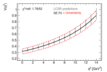
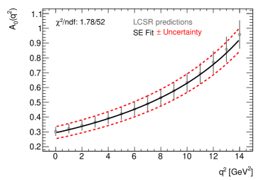
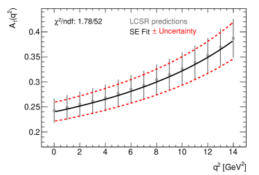
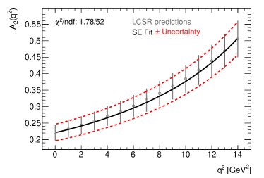
A simultaneous $\chi^{2}$ fit to all sum rule points of Ref. Ball:2004rg assuming the correlations discussed in the previous section is performed. The form factors are parametrized both in the full or in the simplified series expansion, to either linear or quadratic order in $z$, for both the form factor and the helicity amplitude basis. All of them show consistent results, and thus we restrict ourselves to the SE at linear order. In Bharucha:2010im a similar analysis with a less elaborate correlation treatment was performed. We find reasonable agreement with their form factor fit results, but due to the different correlation structure the uncertainties on physical observables differs from this work. The result of the fit to the linear SE is shown in Fig. 2. The central values and uncertainties of the fit were verified using ensembles of pseudo-experiments. (Varying the input assumptions leaves the central values and uncertainties mostly stable, while the resulting correlation matrix is slightly changed as one would expect.) The fitted values for the full series expansion to linear order are listed in Table 5. The corresponding fit parameter correlations are listed in Table 6.

$F$	$a_{0}^{F}$	$a_{1}^{F}$
$A_{0}$	$-0.351\pm 0.032$	$1.250\pm 0.147$
$A_{1}$	$-0.111\pm 0.010$	$-0.208\pm 0.042$
$A_{2}$	$-0.138\pm 0.014$	$0.170\pm 0.049$
$V$	$-0.366\pm 0.034$	$1.148\pm 0.145$

Table 5: Fit result for linear order SE.

	$a_{0}^{V}$	$a_{1}^{V}$	$a_{0}^{A_{0}}$	$a_{1}^{A_{0}}$	$a_{0}^{A_{1}}$	$a_{1}^{A_{1}}$	$a_{0}^{A_{2}}$	$a_{1}^{A_{2}}$
$a_{0}^{A_{0}}$	1.00	-0.86	0.77	0.35	0.74	-0.26	0.78	-0.57
$a_{1}^{A_{0}}$	-0.86	1.00	-0.60	-0.27	-0.58	0.20	-0.61	0.44
$a_{0}^{A_{1}}$	0.77	-0.60	1.00	0.31	0.86	-0.31	0.85	-0.62
$a_{1}^{A_{1}}$	0.35	-0.27	0.31	1.00	0.39	-0.14	0.39	-0.28
$a_{0}^{A_{2}}$	0.74	-0.58	0.86	0.39	1.00	-0.49	0.86	-0.63
$a_{1}^{A_{2}}$	-0.26	0.20	-0.31	-0.14	-0.49	1.00	-0.31	0.22
$a_{0}^{V}$	0.78	-0.61	0.85	0.39	0.86	-0.31	1.00	-0.82
$a_{1}^{V}$	-0.57	0.44	-0.62	-0.28	-0.63	0.22	-0.82	1.00

Table 6: Correlations for linear order SE.

The LCSR result is valid only for small $q^{2}$. However, the $q^{2}$ distribution changes by less than 1% when fitted in the region $q^{2}<7\,\text{GeV}^{2}$ or $q^{2}<14\,\text{GeV}^{2}$ Ball:2004rg . Since the measurements in Ref. Sibidanov:2013rkk are in 4 GeV bins, we restrict ourselves to fitting the data in the range $q^{2}<12\,\text{GeV}^{2}$ to optimize statistical sensitivity while maintaining theoretical validity.

Our fitting procedure can perform a fit to several data sets. In the future, a combined fit to LCSR data, most reliable at low $q^{2}$, and lattice QCD data, most reliable at high $q^{2}$, is desirable. That would constrain the shape of the spectrum in an optimal way, and it would also test the compatibility of the two approaches. Since no reliable and precise lattice QCD calculation of $B\to\rho$ form factors is available, this is left for future work. The framework developed in this work is capable to incorporating such future inputs, which will also allow the whole experimental data set to be used without any restriction on $q^{2}$. Our fitting program is not restricted to $B\rightarrow\rho$ form factors, but can easily be adopted for other processes using the parametrizations discussed.

Figure 3: The differential decay rate as a function of the helicity angles $\cos\theta_{\ell}$ (left), $\cos\theta_{V}$ (middle), and $\chi$ (right), for $\epsilon_{R}=0$ (SM, middle line) and $\epsilon_{R}=\pm 0.15$. The dashed curves show the full series expansion to linear order. The shaded areas correspond to the estimated theoretical uncertainty from the fit to the sum rule prediction, taking into account the full correlation of the expansion coefficients.

IV Predictions of the observables

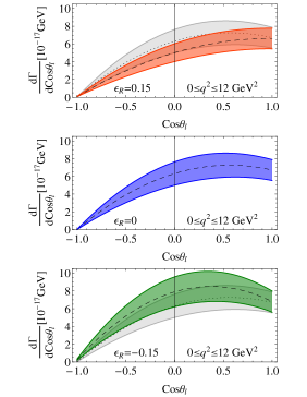
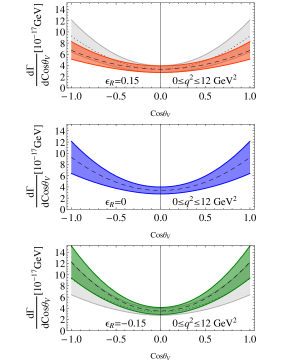
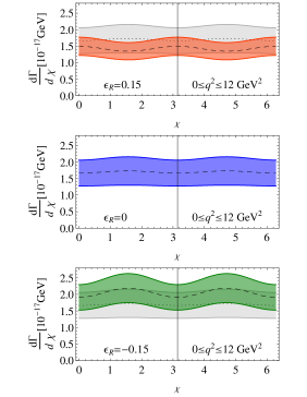
In the following the theoretical predictions using the form factor input and uncertainties from the last section are discussed. The one-dimensional angular distributions including the theoretical uncertainties are displayed in Fig. 3 with $|V_{ub}|=4.2\times 10^{-3}$. The large theoretical uncertainties due to the $B\to\rho$ form factor show the necessity of constructing non-trivial observables to gain sensitivity for right-handed contributions.

The achievable sensitivity of the observables is estimated for 1 ab^-1 and 50 ab^-1 of integrated luminosity, corresponding to the available ${\displaystyle B}\!{\scriptstyle A}{\displaystyle B}\!{\scriptstyle AR}$ and Belle data sets and the anticipated Belle II data. The experimental sensitivities were estimated using the uncertainties of Ref. Sibidanov:2013rkk , assuming that systematic uncertainties in disjoint regions of phase space (e.g. between different bins of $J_{i}$) are fully correlated. For 50 ab^-1 an improvement of the systematic uncertainties of a factor of $3$ is assumed, motivated by the improvements for $B\to X_{u}\ell\bar{\nu}$ from Ref. Aushev:2010bq which face similar experimental challenges. The statistical uncertainties were scaled to correspond to 1 ab^-1 or 50 ab^-1 integrated luminosity. The expected sensitivity for $\epsilon_{R}$ for each observable is characterized as a 68% confidence interval by using the Neyman construction assuming normal distributed uncertainties. In practice, every experiment will have to derive these curves from an ensemble of pseudo-experiments or asymptotic formulae with the specific values of $\epsilon_{R}$ and proper experimental uncertainties incorporated. The sensitivity to a possible right-handed admixture is assessed by the interception of the uncertainty bands with the predicted SM value. Experimental and theoretical uncertainties are assumed to be independent, and addition in quadrature is used to combine them.

IV.1 Forward-backward asymmetry and the two-dimensional asymmetry, $S$

Figure 4: Predictions for the forward-backward asymmetry (left) and $S$ (right), including theoretical uncertainties (blue band), and theory and experimental uncertainties combined in quadrature for 50 ab^-1 (orange) and 1 ab^-1 (green).

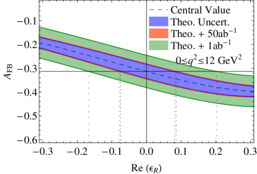
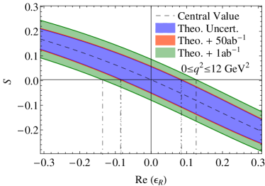
Determining $A_{\rm FB}$ requires the measurements of the decay angle $\theta_{\ell}$ and the predictions including uncertainty estimates are shown in the left panel of Fig. 4. The central value is indicated by dotted lines and the blue band shows the theory uncertainty, as derived in the previous section. The red and green band show the total uncertainties for $1\,{\rm ab}^{-1}$ and $50\,{\rm ab}^{-1}$ of integrated luminosity, and the dashed vertical lines show the expected sensitivities assuming the SM. The theoretical and experimental uncertainties for $1\,{\rm ab}^{-1}$ integrated luminosity are expected to be of similar size. For $50\,{\rm ab}^{-1}$ integrated luminosity the dominant uncertainty will come from the $B\to\rho$ form factor. The sensitivity to New Physics is derived from the slope as a function of $\epsilon_{R}$. For $A_{\rm FB}$ there is only a modest dependence, that reduces significantly for positive admixture, reducing the sensitivity considerably.

The generalized two-dimensional asymmetry, $S$, requires the measurements of the decay angles $\theta_{V,\ell}$. An optimal contour in terms of sensitivity to right-handed admixtures in these angles is devised as follows: The differential decay rate can be rewritten as

$$\frac{\text{d}\Gamma}{\text{d}q^{2}\,\text{d}\cos\theta_{V}\,\text{d}\cos\theta_{\ell}}= \Big{[}f_{\text{SM}}^{(0)}(q^{2},\cos\theta_{\ell})+\epsilon_{R}f_{\text{NP}_{1}}^{(0)}(q^{2},\cos\theta_{\ell})$$

$$+\epsilon_{R}^{2}f_{\text{NP}_{2}}^{(0)}(q^{2},\cos\theta_{\ell})\Big{]}$$

$$+ \Big{[}f_{\text{SM}}^{(1)}(q^{2},\cos\theta_{\ell})+\epsilon_{R}f_{\text{NP}_{1}}^{(1)}(q^{2},\cos\theta_{\ell})$$

$$+ \epsilon_{R}^{2}f_{\text{NP}_{2}}^{(1)}(q^{2},\cos\theta_{\ell})\Big{]}\cos^{2}\theta_{V}\,,$$ (24)

where the functions $f^{(n)}_{i}$ are second order polynomials in $\cos\theta_{\ell}$ and depend on $q^{2}$ explicitly, as well as indirectly through the form factors

$$f^{(0)} =J_{1s}+J_{2s}+J_{6s}\cos\theta_{\ell}-2J_{2s}\cos^{2}\theta_{\ell}\,,$$

$$f^{(1)} =J_{1c}+J_{2c}-J_{1s}-J_{2s}+(J_{6c}-J_{6s})\cos\theta_{\ell}$$

$$\phantom{=}+2(J_{2s}-J_{2c})\cos^{2}\theta_{\ell}\,.$$ (25)

Treating $\epsilon_{R}$ as a small parameter, Eq. (9) becomes

$$A =A_{\text{SM}}+\epsilon_{R}\,A_{\text{NP}_{1}}+\epsilon_{R}^{2}\,A_{\text{NP}_{2}}\,,$$

$$B =B_{\text{SM}}+\epsilon_{R}\,B_{\text{NP}_{1}}+\epsilon_{R}^{2}\,B_{\text{NP}_{2}}\,,$$ (26)

$$S =\frac{A_{\text{SM}}-B_{\text{SM}}}{A_{\text{SM}}+B_{\text{SM}}}+2\epsilon_{R}\,\frac{A_{\text{NP}_{1}}B_{\text{SM}}-A_{\text{SM}}B_{\text{NP}_{1}}}{(A_{\text{SM}}+B_{\text{SM}})^{2}}+\ldots\,.$$

In the following we require $S_{\text{SM}}\approx 0$ what approximately divides the phase-space equally in the two regions of the asymmetry. The sensitivity to $\epsilon_{R}$ is optimized by demanding a maximal slope,

$$\frac{\text{d}S}{\text{d}\epsilon_{R}}=2\,\frac{A_{\text{NP}_{1}}B_{\text{SM}}-A_{\text{SM}}B_{\text{NP}_{1}}}{(A_{\text{SM}}+B_{\text{SM}})^{2}}+{\cal O}(\epsilon_{R})\,.$$ (27)

This implies that

$$A_{\text{SM}} \approx B_{\text{SM}}\,,$$

$$A_{\text{NP}_{1}} \gg B_{\text{NP}_{1}}\quad\text{or}\quad A_{\text{NP}_{1}}\ll B_{\text{NP}_{1}}\,.$$ (28)

In addition, the SM left-handed and the NP right-handed couplings are odd and even in $\cos\theta_{\ell}$, and both are symmetric in $\cos\theta_{V}$. The dividing curves are derived as follows. The SM and NP differential distribution are separated along a curve of constant ratio, causing a deviation in ration in the presence of non negligible right-handed admixture. The symmetry in $\cos\theta_{V}$ forces one region to be within $\pm\cos\theta_{V}(\cos\theta_{\ell})$ with $\cos\theta_{V}(\cos\theta_{\ell}^{\text{min}})=0$. The first relation $\text{d}\Gamma_{\text{SM}}=\kappa\,\text{d}\Gamma_{\text{NP}}^{(1)}$ using (24) is written as

$$\int_{\Delta q^{2}}\text{d}q^{2}\big{[}f_{\text{SM}}^{(0)}+f_{\text{SM}}^{(1)}\cos^{2}\theta_{V}\big{]}$$

$$=\int_{\Delta q^{2}}\text{d}q^{2}\kappa\big{[}f_{\text{NP}_{1}}^{(0)}+f_{\text{NP}_{1}}^{(1)}\cos^{2}\theta_{V}\big{]}\,,$$ (29)

where arguments for $(q^{2},\cos\theta_{\ell})$ were suppressed for the $f$ functions for brevity. This implies

$$\cos^{2}\theta_{V}(\cos\theta_{\ell})=\frac{\int_{\Delta q^{2}}\big{[}\kappa f_{\text{NP}_{1}}^{(0)}-f_{\text{SM}}^{(0)}\big{]}\text{d}q^{2}}{\int_{\Delta q^{2}}\big{[}-\kappa f_{\text{NP}_{1}}^{(1)}+f_{\text{SM}}^{(1)}\big{]}\text{d}q^{2}}\,.$$ (30)

From this immediately follows

$$\cos\theta_{V}^{\text{min,max}}(\cos\theta_{\ell})=\pm\sqrt{\frac{\int_{\Delta q^{2}}\big{[}\kappa f_{\text{NP}_{1}}^{(0)}-f_{\text{SM}}^{(0)}\big{]}\text{d}q^{2}}{\int_{\Delta q^{2}}\big{[}-\kappa f_{\text{NP}_{1}}^{(1)}+f_{\text{SM}}^{(1)}\big{]}\text{d}q^{2}}}\,.$$ (31)

The minimal value for $\cos\theta_{\ell}^{\text{min}}$ can be numerically obtained via

$$\int_{\Delta q^{2}}\text{d}q^{2}\big{[}\kappa f_{\text{NP}_{1}}^{(0)}(q^{2},\cos\theta_{\ell}^{\text{min}})\big{]} =\int_{\Delta q^{2}}\text{d}q^{2}\big{[}f_{\text{SM}}^{(0)}(q^{2},\cos\theta_{\ell}^{\text{min}})\big{]}\,.$$ (32)

Note that the $f_{i}$ functions may be negative and thus the minimum value cannot be imposed by having the integrand zero. Thus $\cos\theta_{\ell}^{\text{min}}$ will depend on the interval $\Delta q^{2}$ and one numerically has $\cos\theta_{\ell}^{\text{min}}=-0.611$. Independent of the actual form factor shape, for $\cos\theta_{V}=1$ one has

$$\kappa f_{\text{NP}_{1}}^{(0)}-f_{\text{SM}}^{(0)}=-\kappa f_{\text{NP}_{1}}^{(1)}+f_{\text{SM}}^{(1)}\,,$$ (33)

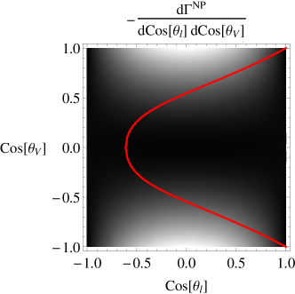
so that $\cos\theta_{\ell}^{\text{max}}=1$ and $\kappa$ is determined by requiring $S_{\text{SM}}\approx 0$. The resulting curve most sensitive for $\epsilon_{R}$ that separates regions $A$ and $B$ can be numerically approximated by

$$\cos\theta_{V}=\pm\sqrt{\frac{0.8472\cos^{2}\theta_{\ell}+1.9038\cos\theta_{\ell}+0.8472}{-1.1484\cos^{2}\theta_{\ell}+1.9038\cos\theta_{\ell}+2.8429}}\,.$$ (34)

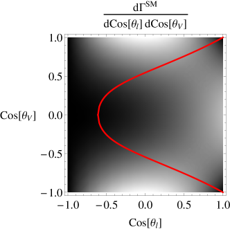
This choice depends on nonperturbative input quantities. However, it turns out that in the heavy quark limit the minimum value $\cos\theta_{\ell}^{\text{min}}$ is given form-factor independently and agrees well with the one derived from the full form factors, while the shape $\cos\theta_{V}$ ($\cos\theta_{\ell}$) is distorted mildly using the heavy quark limit form factors. This curve is displayed together with the SM and NP density distributions in Fig. 5.

The Neyman belt of $S$ and sensitivities are shown in Fig. 4: integrating over a range of $q^{2}$ introduces additional uncertainties, that do not cancel entirely in the ratio, resulting in larger theoretical uncertainties than for $A_{\rm FB}$. The overall sensitivity on NP for $1\,{\rm ab}^{-1}$ of integrated luminosity, however, is better due to the increased dependence on $\epsilon_{R}$, and for $50\,{\rm ab}^{-1}$ of data the sensitivity is comparable.

Figure 5: The optimized contour (red curve) separating the SM (left) and NP linear in $\epsilon_{R}$ (right) contributions.

IV.2 Simple generalized ratios

Figure 6: The most sensitive angular observables to ${\rm Re}\,\epsilon_{R}$ (top row) and to ${\rm Im}\,\epsilon_{R}$ (lower row), assuming $\epsilon_{R}$ to be purely real or imaginary, respectively. The blue bands show the theoretical uncertainties, while the orange [dark-green] bands show theory and experimental uncertainties combined in quadrature, for 50 ab^-1 [1 ab^-1] of $B$-factory data. The observables, $\langle P_{1}\rangle$ (top left), $\langle P_{5}^{\prime}\rangle$ (top center), $\langle P_{5,4}\rangle$ (top right), $\langle P_{8,5}\rangle$ (lower left), $\langle P_{9,5}\rangle$ (lower center), $\langle P_{8,3}\rangle$ (lower right), are defined in Eqs. (11)–(14).

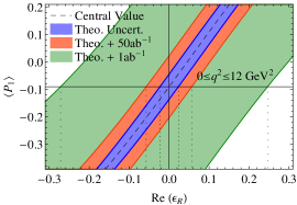
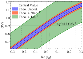
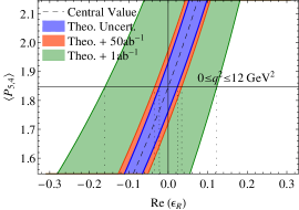
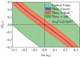
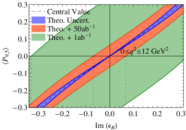
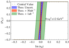
In the context of “clean observables” a set of simple generalized observables, $P_{i}$, in Eq. (11-14), from which one expects the best theoretical sensitivity are derived. The most sensitive observables in the context of real right-handed currents, are $\langle P_{1}\rangle$, $\langle P_{5}^{\prime}\rangle$ and $\langle P_{5,4}\rangle$. The most sensitive observables for imaginary right-handed contributions are $\langle P_{8,5}\rangle$, $\langle P_{9,5}\rangle$ and $\langle P_{8,3}\rangle$. The corresponding predictions and sensitivities are shown in Fig. 6. The statistical correlations between the numerator and denominator in the observables was estimated using Monte Carlo methods, neglecting any influence from background. The three-dimensional observables reduce the theoretical uncertainties with respect to the one-dimensional or two-dimensional asymmetries. Their experimental uncertainties, however, are larger due to the great number of free parameters that need to be determined from the same data. The most precise observable for $1\,{\rm ab}^{-1}$ of integrated luminosity are $\langle P_{5,4}\rangle$ and $\langle P_{8,3}\rangle$, for real and imaginary $\epsilon_{R}$, respectively.

IV.3 Testing NP contributions vs. form factor uncertainties

The predicted value of the observables depends on the assumed form factor shape and integrated $q^{2}$ range. As this is a nonperturbative calculation with possible unknown systematic uncertainties, in case experimentally a significant deviation is observed, it is necessary to verify if NP is the source of a possible deviation (see the recent discussion related to $B\to K^{*}$ transitions Jager:2012uw ).

An obvious consistency check is to measure several of the presented observables. In addition one should perform a $q^{2}$ binned analysis of these, for instance reconstruct them in a high $q^{2}$ and a low $q^{2}$ range. If a measured deviation is related to not properly considered theoretical or also experimental uncertainties, it will produce an inconsistent pattern, since one expects all regions in $q^{2}$ to show a consistent deviation form the SM due to a right-handed admixture.

In addition two of the “clean observables”, $\langle P_{4}\rangle$ and $\langle P_{5}\rangle$, are nearly independent of a right-handed current,

$$\langle P_{4}\rangle_{\text{bin}} =\frac{\sqrt{2}\int_{\Delta q^{2}}\text{d}q^{2}J_{4}}{\sqrt{-\int_{\Delta q^{2}}\text{d}q^{2}J_{2c}\,\,\int_{\Delta q^{2}}\text{d}q^{2}(2J_{2s}-J_{3})}}\,,$$

$$\approx 0.94\pm 0.01_{\text{Theory}}\,,$$ (35)

$$\langle P_{5}\rangle_{\text{bin}} =\frac{\int_{\Delta q^{2}}\text{d}q^{2}J_{5}}{\sqrt{-\int_{\Delta q^{2}}\text{d}q^{2}2J_{2c}\,\,\int_{\Delta q^{2}}\text{d}q^{2}(2J_{2s}+J_{3})}}$$

$$\approx 0.95\pm 0.01_{\text{Theory}}\,.$$ (36)

Thus a global hypothesis test incorporating all observables, taking into account the proper experimental and theoretical correlations, would be desirable and be the most powerful test of the data for the presence of right-handed currents.

Note that $\langle P_{4}\rangle$ is also insensitive to ${\rm Im}\,\epsilon_{R}$, while there is a quadratic effect in $\langle P_{5}\rangle$. This happens to be a coincidence in cancellation of the NP parameters in the point-by-point ratio, which is broken by the finite binning. However, numerically this breaking amounts to a very small, unobservable effect. In case these $P_{i}$ can be measured using for instance the asymmetries in Table. 3, one can use this prediction to test for other effects.

V Global fit for $|V_{ub}^{L}|$ and $\epsilon_{R}$

The estimated sensitivities on $\epsilon_{R}$ in the previous section can be used to add an orthogonal constraint to the global fit performed in Section I. The gain in overall sensitivity on $|V_{ub}^{L}|$ and $\epsilon_{R}$ is estimated by extrapolating the experimental uncertainties to $1\,{\rm ab}^{-1}$ and $50\,{\rm ab}^{-1}$. For the branching fraction input other than $B\to\rho\ell\bar{\nu}$ and $B\to\pi\ell\bar{\nu}$ the projections from Ref. Aushev:2010bq are used. For $B\to\pi\,\ell\bar{\nu}$ a more optimistic uncertainty of $3\%$ is used due to estimated progress in the lattice QCD form factor determinations USlqcd . For the $B\to\rho\ell\bar{\nu}$ branching fraction the uncertainties discussed in Section IV are used and are listed in Table 7. The irreducible uncertainty of the $B\to\rho\,\ell\bar{\nu}$ form factors is quoted to be 7% in Ref. Ball:2004rg . In the following no such scenarios are explored, due to the complication related to how a reduction of uncertainty would affect the overall correlations between the different form factors.

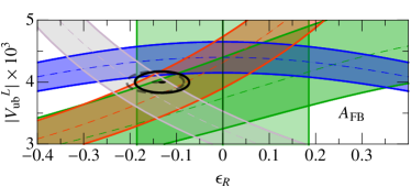
Fig. 7 shows the results for the simultaneous fit for $|V_{ub}^{L}|$ and $\epsilon_{R}$ for integrated luminosities of $1\,{\rm ab}^{-1}$ and $50\,{\rm ab}^{-1}$. The fits incorporate the expected constraints from either $A_{\text{\rm FB}}$, $S$, or $P_{5,4}^{\prime}$ in the absence of right-handed currents. For the $1\,{\rm ab}^{-1}$ scenario, the current experimental central values are used for $|V_{ub}|$, whereas for $50\,{\rm ab}^{-1}$ the SM is assumed, with identical $|V_{ub}|$ from all channels. For $1\,{\rm ab}^{-1}$ $B$-factory data, $S$ results in the largest gain in sensitivity for right-handed currents among the studied observables. Table 8 lists the reduction of the uncertainty of $|V_{ub}^{L}|$ and $\epsilon_{R}$ with respect to a fit without any additional orthogonal bound. Although the theoretical uncertainties on $S$ are more sizable than on $P_{5,4}^{\prime}$, the experimental simplicity of the two-dimensional asymmetry results in the best overall expected sensitivity. The reduction in experimental uncertainties for $50\,{\rm ab}^{-1}$ statistics changes this picture: here the theoretical uncertainties on the $B\to\rho$ form factors dominate the overall uncertainty of all observables and $P_{5,4}^{\prime}$ results in the best expected sensitivity.

Figure 7: The $\chi^{2}$ fits for $|V_{ub}^{L}|$ and $\epsilon_{R}$ assuming $1\,{\rm ab}^{-1}$ (left) and $50\,{\rm ab}^{-1}$ (right) of $B$-factory data. The green bands show the $B\to\rho\ell\bar{\nu}$ information, c.f., Fig. 1. The observable used for the expected orthogonal bound on $\epsilon_{R}$, assuming the SM, is shown in each Figure. The used uncertainties for $50\,{\rm ab}^{-1}$ are quoted in Tables 7. Table 8 lists the improvement in uncertainty by including the orthogonal constraint from the discussed observable on $\epsilon_{R}$ with respect to the uncertainty of fitting the experimental information available by $B\to X_{u}\ell\bar{\nu}$, $B\to\tau\bar{\nu}$, $B\to\pi\ell\bar{\nu}$, and $B\to\rho\ell\bar{\nu}$ only.

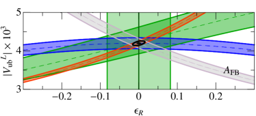
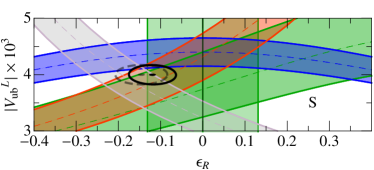
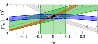
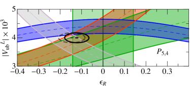
Decay	Expected error on $|V_{ub}|$
$B\to\pi\,\ell\bar{\nu}$	3%
$B\to X_{u}\ell\bar{\nu}$	3%
$B\to\tau\,\bar{\nu}_{\tau}$	1.5%
Decay	Expected error on $\mathcal{B}$
$B\to\rho\,\ell\bar{\nu}$	3%

Table 7: The assumed uncertainties on $|V_{ub}|$ and $\mathcal{B}(B\to\rho\ell\bar{\nu}$ for $50\,{\rm ab}^{-1}$ of integrated luminosity are listed.

Fit	$\delta\left(\left|V_{ub}^{L}\right|\right)$ [%]	$\delta\left(\epsilon_{R}\right)$ [%]
4 modes + $A_{\text{FB}}$ (1 ab-1)	$-0.3$	$-5$
4 modes + $S$ (1 ab-1)	$-0.5$	$-9$
4 modes + $P_{5,4}$ (1 ab-1)	$-0.5$	$-8$
4 modes + $A_{\text{FB}}$ (50 ab-1)	$-0.4$	$-2$
4 modes + $S$ (50 ab-1)	$-0.5$	$-2$
4 modes + $P_{5,4}$ (50 ab-1)	$-3$	$-10$

Table 8: The expected relative reduction in the uncertainty of $\left|V_{ub}^{L}\right|$ and $\epsilon_{R}$ for the $\chi^{2}$ fits in Figs. 7. The improvements are quoted with respect to the expected uncertainties on the 4-mode analysis for 1 ab^-1 and 50 ab^-1, which are $\Delta\left(\left|V_{ub}^{L}\right|\times 10^{3},\Delta\epsilon_{R}\right)=\left(0.18,0.061\right)$ and $\left(0.06,0.016\right)$, respectively.

VI Summary and Conclusions

In this paper, the full decay distribution in semileptonic $B\to\rho[\rightarrow\pi\pi]\ell\bar{\nu}$ decay was analyzed to explore the consequences of a possible right-handed semileptonic current from physics beyond the Standard Model. A number of observables was explored, some new and some defined in the literature, and a detailed investigation of the impact of the theoretical uncertainties on the sensitivity was performed.

The theoretical uncertainties and correlations are crucial ingredients of predicting the uncertainties of the observables reliably. Such correlation information is not readily available in existing $B\to\rho$ or other form factor calculations. A model of these correlations is discussed for the $B\to\rho$ form factor, incorporating correlations among different form factors and different $q^{2}$ points of the form factors

A detailed analysis on the $B\to\rho$ form factor was performed. The use of unitarity constraints to predict the form factor shape up to a small expansion was revisited and verified In the context of a vector meson final state. This technique is known in the literature as $z$-parametrization, and has the advantage to be valid over the entire $q^{2}$ range of the form factor. In order to combine all this information, a fit routine was developed, which is capable of fitting several correlated or uncorrelated sources of form factor values, i.e., LCSR and lattice QCD, taking into account the correlations among the form factors and among different points of $q^{2}$. The fit results have been cross-checked with several parametrizations and validated by fits of pseudo-input.

With the theoretical prediction for the fully differential spectrum including correlations at hand, the sensitivity to a right-handed current was investigated, which has been proposed as a possibility to ease a current tensions in the determinations of $|V_{ub}|$. To set a bound on this beyond Standard Model contribution, two approaches are possible: (i) a full four-dimensional fit for the $J_{i}$ coefficients or counting experiments that involve determining the partial branching fraction in several regions of phase space and combining this information appropriately to project out either the $J_{i}$ coefficients, or (ii) to construct asymmetries sensitive to NP contributions. The latter offer an obvious alternative, since with the currently available $B$-factory data, a full four-dimensional fit appears to be a very challenging endeavor.

The discussed observables exhibit very different theoretical and experimental uncertainties: besides the usual forward-backward asymmetry, a two-dimensional generalized asymmetry is proposed by integrating out one of the decay angles form the fully differential decay rate. These two are experimentally the simplest observables. A set of generalized three-dimensional observables is discussed. These are experimentally more challenging, and the eventual observables involve ratios of statistically and systematically correlated observables.

A ranking in terms of sensitivity reveals that the balance of experimental and theoretical uncertainties is important: for the available $B$-factory statistics of about $1\,{\rm ab}^{-1}$, the two dimensional asymmetry $S$ with its simple experimental definition seems to be the most sensitive to the presence of right-handed currents. For the anticipated $50\,{\rm ab}^{-1}$ Belle II statistics, the more complicated three-dimensional observables result in the best expected sensitivity due to the reduction of experimental uncertainties. A direct determination of $\epsilon_{R}$ allows to introduce an orthogonal constraint into the indirect determination involving $\left|V_{ub}\right|$ measurements from various decays with different $\epsilon_{R}$ dependencies. Including the most sensitive direct $\epsilon_{R}$ constraint for $1\,{\rm ab}^{-1}$ or $50\,{\rm ab}^{-1}$, reduces the uncertainty of $\epsilon_{R}$ by about 10% in such a global analysis. This implies that even with the current $B$-factory datasets a useful statement about $\epsilon_{R}$ from $B\to\rho\ell\nu$ can be obtained.

In case a deviation from the SM is observed, a global hypothesis test incorporating all observables is desirable: the presence of a right-handed admixture should result in a consistent change. A non-consistency could imply problems with the predictions of the $B\to\rho$ form factors. To assert the correctness of the form factor predictions, an analysis in bins of $q^{2}$ (e.g., a low and high $q^{2}$ region) should be performed to see if the deviation is consistent and independent of the $q^{2}$ region. Ultimately a fully differential analysis by a four dimensional fit would be desirable to analyze the full anatomy of this decay mode. In the context of such an analysis, the nonperturbative uncertainties would be greatly reduced.

Future high statistics $B\to\rho\ell\bar{\nu}$ measurements will not only allow the extraction of the $J_{i}$ coefficients in this semileptonic decay and more sensitive searches for right-handed current, it can also be used to test the form factor relations, which are important for the interpretation of the identically defined observables in $B\to K^{*}\ell^{+}\ell^{-}$. If precise and reliable lattice QCD calculations of $B\to\rho$ and $B\to K^{*}$ form factors become available, the quoted theoretical uncertainties can be greatly reduced. Such additional inputs can be readily incorporated into our fit for the form factors and the combined analysis with the available experimental data. Furthermore, precise form factor input at high $q^{2}$ would allow to access the whole kinematic region, increasing the statistical power of the experimental data and hence improving the sensitivity to new physics in $B\to\rho\ell\bar{\nu}$.

Appendix A Partially Integrated Angular Rates

The differential rates integrated over one angle are then given by

$$\frac{\text{d}\Gamma}{\text{d}\cos\theta_{V}\,\text{d}\cos\theta_{\ell}} =\frac{G_{F}^{2}|V_{ub}^{L}|^{2}m_{B}^{3}}{\pi^{3}}\bigg{\{}\bar{J}_{1s}\sin^{2}\theta_{V}+\bar{J}_{1c}\cos^{2}\theta_{V}+(\bar{J}_{2s}\sin^{2}\theta_{V}+\bar{J}_{2c}\cos^{2}\theta_{V})\cos 2\theta_{\ell}$$

$$+(\bar{J}_{6s}\sin^{2}\theta_{V}+\bar{J}_{6c}\cos^{2}\theta_{V})\cos\theta_{\ell}\bigg{\}}\,,$$ (37)

$$\frac{\text{d}\Gamma}{\text{d}\cos\theta_{V}\,\text{d}\chi} =\frac{G_{F}^{2}|V_{ub}^{L}|^{2}m_{B}^{3}}{\pi^{4}}\bigg{\{}(\bar{J}_{1s}\sin^{2}\theta_{V}+\bar{J}_{1c}\cos^{2}\theta_{V})-\frac{1}{3}(\bar{J}_{2s}\sin^{2}\theta_{V}+\bar{J}_{2c}\cos^{2}\theta_{V})$$

$$+\frac{2}{3}\bar{J}_{3}\sin^{2}\theta_{V}\,\cos 2\chi+\frac{\pi}{4}\bar{J}_{5}\sin 2\theta_{V}\,\cos\chi+\frac{\pi}{4}\bar{J}_{7}\sin 2\theta_{V}\,\sin\chi+\frac{2}{3}\bar{J}_{9}\sin^{2}\theta_{V}\,\sin 2\chi\bigg{\}}\,,$$ (38)

$$\frac{\text{d}\Gamma}{\text{d}\cos\theta_{\ell}\,\text{d}\chi} =\frac{G_{F}^{2}|V_{ub}^{L}|^{2}m_{B}^{3}}{3\pi^{4}}\times\bigg{\{}2\bar{J}_{1s}+\bar{J}_{1c}+(2\bar{J}_{2s}+\bar{J}_{2c})\cos 2\theta_{\ell}+2\bar{J}_{3}\sin^{2}\theta_{\ell}\,\cos 2\chi$$

$$+(2\bar{J}_{6s}+\bar{J}_{6c})\cos\theta_{\ell}+2\bar{J}_{9}\sin^{2}\theta_{\ell}\,\sin 2\chi\bigg{\}}\,.$$ (39)

Integrating over two angles, the rates become

$$\frac{\text{d}\Gamma}{\text{d}\cos\theta_{\ell}} =\frac{2G_{F}^{2}|V_{ub}^{L}|^{2}m_{B}^{3}}{3\pi^{3}}\bigg{\{}2\bar{J}_{1s}+\bar{J}_{1c}(+2\bar{J}_{2s}+\bar{J}_{2c})\cos 2\theta_{\ell}+(2\bar{J}_{6s}+\bar{J}_{6c})\cos\theta_{l}\bigg{\}}\,,$$ (40)

$$\frac{\text{d}\Gamma}{\text{d}\cos\theta_{V}\,} =\frac{2G_{F}^{2}|V_{ub}^{L}|^{2}m_{B}^{3}}{\pi^{3}}\bigg{\{}\bar{J}_{1s}\sin^{2}\theta_{V}+\bar{J}_{1c}\cos^{2}\theta_{V}-\frac{1}{3}(\bar{J}_{2s}\sin^{2}\theta_{V}+\bar{J}_{2c}\cos^{2}\theta_{V})\bigg{\}}\,,$$ (41)

$$\frac{\text{d}\Gamma}{\text{d}\chi} =\frac{G_{F}^{2}|V_{ub}^{L}|^{2}m_{B}^{3}}{2\pi^{4}}\bigg{\{}\frac{8}{3}\bar{J}_{1s}+\frac{4}{3}\bar{J}_{1c}-\frac{8}{9}\bar{J}_{2s}+\frac{4}{9}\bar{J}_{2c}+\frac{16}{9}\bar{J}_{3}\,\cos 2\chi+\frac{16}{9}\bar{J}_{9}\,\sin 2\chi\bigg{\}}\,.$$ (42)

Appendix B Branch Cut Uncertainty

Using $t\equiv q^{2}$, the bound on the expansion coefficients of the form factors $A_{l}^{X}$ can be written as Bharucha:2010im

$$\frac{1}{2\pi}\int_{0}^{2\pi}\text{d}\phi\left|\Phi A_{l}^{X}\right|^{2}(e^{-i\phi})\leq 1\,,$$ (43)

where $A_{l}^{X}$ are projections onto the longitudinal $(l)$ and transverse $(t)$ components, $|A_{l}^{X}(t)|^{2}=P_{l}^{\mu\nu}\langle\rho|j_{\mu}^{X}|B\rangle\langle B|j_{\nu}^{X}|\rho\rangle\,.$ For our model we need to redefine the kinematical factor with poles in the branch cut region into the matrix element $|A_{l}^{X}(t)|^{2}\to\frac{(t_{-}-t)(t_{+}-t)}{3t}|\widetilde{A}_{l}^{X}(t)|^{2}$. Hence the $\Phi$ function is now given by $\Phi_{\text{new}}(t)=\sqrt{3\frac{-t}{z(t,0)}\frac{t_{-}-t}{z(t,t_{-})}(t-t_{+})}\Phi_{F}(t)$. Analyticity is restored by subtracting the branch cut

$$g(z) \equiv\Phi(z)\bar{A}_{l}^{X}(z)=\Phi_{\text{new}}(z)\widetilde{A}_{l}^{X}(z)$$

$$\quad-\frac{1}{\pi}\int_{-1}^{z_{\text{cut}}}\text{d}x\,\frac{\Phi_{\text{new}}(x)\,\text{Im}F(x)}{x-z}\,.$$ (44)

The true analytic form factor is $\bar{A}_{l}^{X}(z)$, for which we can derive the bound using $g(z)$. Here $z_{\text{cut}}\equiv z(t_{\text{cut}},t_{0})$ is the position of the lowest sub-threshold branch cut. We integrate only from $z\equiv z(t_{+},t_{0})=-1$, because everything above the two-particle threshold is being taken care of already. The function $\text{Im}\,F(x)$ is connected to the branch cut, and no analytic expression of this exists. However we may model it with an ansatz, since its origin is related to matrix elements of the form $\text{Im}\,\,\langle 0|j^{X}|Bh\rangle$, where $h$ is a (combination) of allowed light hadrons in the final state. This is an intermediate state of the transition $B\to\rho$. The model function should fulfill the conditions (i) vanish as $t\to\infty$ (or get constant for a finite $t$ interval), (ii) start with zero at the threshold point, and (iii) it should be a contiguous function. We will model this function inspired by the optical theorem and saturation of the lowest states due to phase-space and multiplicity suppression. The first factor is related to the “production coupling” of the state, and the second is related to the kinematics of the branch cut.

We try a model function inspired by $e^{+}e^{-}\to\mu^{+}\mu^{-}$ scattering, which gives larger contributions than, e.g., a model used in Caprini:1995wq

$$\text{Im}F(t)=C\sqrt{t_{+}}\sqrt{1-\frac{t_{\text{cut}}}{t}}\left(1+\frac{t_{\text{cut}}}{2t}\right),\,\quad t_{\text{cut}}\leq t\leq t_{+}\,,$$ (45)

where $C$ is in general a dimensionless quantity. The saturation of the lowest state has been assumed in a dispersion relation as $\text{Im}\,\,\langle 0|j^{X}|Bh\rangle$ to estimate $C$ Caprini:1995wq . Integrating over the phase-space region in question, the authors have found a slow varying number of order one. Another possibility is to assume the on-shell production of the leading branch-cut state out of the vacuum. We use a generic meson coupling constant model in the narrow width approximation. We normalize the production current to the threshold mass of the system over the width, similarly to an intermediate on-shell state. Each additional particle has a phase-space suppression factor of $1/(4\pi)^{2}$. We neglect further suppression by spin and isospin quantum numbers, i.e., Clebsch-Gordan coefficients. We estimate the coupling constant by the relation

$$C \approx\frac{g_{Bn\pi}^{2}(m_{B}+n\,m_{\pi})}{\Gamma_{B\pi\pi}(16\pi^{2})^{n-1}}\,c\,\overset{\overset{\text{narrow}}{\text{\tiny width}}}{\underset{n=2}{\longrightarrow}}\,\frac{3}{\pi}\frac{1+\frac{2m_{\pi}}{m_{B}}}{(1-\frac{4m_{\pi}^{2}}{m_{B}^{2}})^{\frac{3}{2}}}\,c$$ (46)

with a dimensionless constant $c\sim{\cal O}(1)$. The coupling gets smaller for a higher multiplicity state, as expected, and we focus on the leading contribution $n=2$.

In some cases, there may be additional suppressions, e.g., for isospin violating transitions or OZI-suppressed decays, leading to a smaller coupling $C$. This could happen in $B_{c}$ decays, however it is not present in $B\to\rho$.

This most important contribution will be from $B+2\pi$, with $n=2$, which is neither isospin, nor spin nor OZI suppressed. Numerically we have

$$t_{+}\approx 36.65\,\text{GeV}^{2}\quad t_{\text{cut}}\approx 30.79\,\text{GeV}^{2}\quad z_{\text{cut}}\approx-0.344\,.$$

For comparison the physical form factor values are $z(0,t_{0})\approx 0.10\,,\,z(t_{-},t_{0})\approx-0.10\,.$ In summary we estimate in our approach $C\approx 1.01c$, hence an order one number as as in Caprini:1995wq . Subsequently we will assume a (hopefully) conservative estimate of $C\approx 10$.

For the estimate of this branch cut influence, we use the Minkowski inequality, which states for (Lebesgue) integrable functions $||f+g||_{p}\leq||f||_{p}+||+g||_{p}$ for any norm $p>1$, which is defined as $||f||_{p}=\left(\int\text{d}\mu|f|^{p}\right)^{\frac{1}{p}}\,.$ Thus for $p=2$ in our case we can write the inequality (43) as

$$\sqrt{\int_{0}^{2\pi}\text{d}\phi\left|\Phi\widetilde{A}_{l}^{X}\right|^{2}(e^{-i\phi})}\leq\sqrt{\int_{0}^{2\pi}\text{d}\phi\left|g(e^{-i\phi})\right|^{2}}$$

$$\phantom{\leq\,}\,+\sqrt{\int_{0}^{2\pi}\text{d}\phi\left|\frac{1}{\pi}\int_{-1}^{z_{\text{cut}}}\text{d}x\,\,\frac{\Phi(x)\,\text{Im}F(x)}{x-e^{-i\phi}}\right|^{2}}$$

$$\leq\sqrt{2\pi}(1+I_{\text{cut}})\,.$$ (47)

We have used the fact, that the integral of the analytic function $g(z)$ fulfills the bound, while the left-hand side is the “true” relation. Hence we can estimate the deviation from the bound through this additional cut removal function by the model and numerical integration. For the numerical evaluation we take two subtractions $n=2$, as the contributing form factors require these numbers of subtractions. Furthermore we need to use a numerical value for $\chi(n=2)$. Since this has not been calculated by us, we take the value for the transverse form factor part with two subtractions from Bharucha:2010im with $\chi(2)=0.0116/m_{b}^{2}$. For this being a rough estimate of the branch cut uncertainty, this value will be sufficient.

In fact we derived an indirect correction to the bound, which constrains the expansion parameters of the residual $q^{2}$ dependence. Our calculated form factor dependence thus fulfills the corrected bound

$$\frac{1}{2\pi}\int_{0}^{2\pi}\text{d}\phi\left|\Phi A_{l}^{X}\right|^{2}(e^{-i\phi}) =\frac{1}{B_{FF}\,\Phi_{FF}}\,\sum_{k=0}^{K}\alpha^{FF}_{k}\,z(q^{2},\,q^{2}_{0})^{k}$$

$$\leq(1+I_{\text{cut}})^{2}\,,$$ (48)

which has a correction term of the form $2I_{\text{cut}}+I_{\text{cut}}^{2}$. If these additional terms are sufficiently small, the bound on the residual dependence is not changed dramatically and from this we conclude the shape is not changed by these branch cut singularities. Note especially that the leading contribution to $\alpha_{0}$ is only a constant shift, and no shape distortion. A modification of the first shape influencing expansion coefficient would be multiplied by a number $|z|\lesssim 0.1$. Numerically this amounts to

$$I_{\text{cut}} =\sqrt{\frac{1}{2\pi}\int_{0}^{2\pi}\text{d}\phi\left|\frac{1}{\pi}\int_{-1}^{z_{\text{cut}}}\text{d}x\,\,\frac{\Phi(x)\,\text{Im}F(x)}{x-e^{-i\phi}}\right|^{2}}I_{\text{cut}}\approx 0.11\,.$$ (49)

This now has to be compared with the bound

$$\frac{1}{2\pi}\int_{0}^{2\pi}\text{d}\phi\left|\Phi A_{l}^{X}\right|^{2}(e^{-i\phi})\leq(1+I_{\text{cut}})^{2}\,,$$ (50)

At first sight, this seems to indicate an order ${\cal O}(10\%)$ correction to the form factor bound itself. However, that will affect the bound on all expansion coefficients, and does not mean a 10% contribution to the leading coefficient squared of all of the form factors. For the expansion parameter fulfills $-0.1\lesssim z\lesssim 0.1$, and so the larger allowance of higher order coefficient contributions will not change the slope dramatically. Furthermore it has to be compared with the ${\cal O}(10\%)$ uncertainty of each form factor data point, which is of the same order of magnitude. Furthermore this bound constraints a linear combination of all transverse form factors, which can formally easy be derived in the helicity eigenbasis. So in total even with this correction only a mild influence on the individual form factor shape is expected.

In Ref. Caprini:1995wq a similar model, which gives smaller numbers in this case, was applied to the $B\to D^{*}\ell\bar{\nu}_{\ell}$ decay in a slightly different approach. The have found a $10^{-3}\cdot C$ influence on the shape parameters, which they dubbed to be very small. This is to be compared to our numbers, which are a bit higher as expected but still ok.

Thus we conclude the influence of branch cuts is at most at the few percent level on the form factor shape as well as the parametrization. Therefore regarding our precision, this effect can be safely neglected.

References

- (1) J. Charles, S. Descotes-Genon, Z. Ligeti, S. Monteil, M. Papucci and K. Trabelsi, Phys. Rev. D 89, 033016 (2014) [arXiv:1309.2293 [hep-ph]].
- (2) A. Crivellin, Phys. Rev. D 81, 031301 (2010) [arXiv:0907.2461 [hep-ph]].
- (3) A. J. Buras, K. Gemmler and G. Isidori, Nucl. Phys. B 843, 107 (2011) [arXiv:1007.1993 [hep-ph]].
- (4) R. Feger, T. Mannel, V. Klose, H. Lacker and T. Luck, Phys. Rev. D 82 (2010) 073002 [arXiv:1003.4022 [hep-ph]].
- (5) S. Faller, T. Mannel and S. Turczyk, Phys. Rev. D 84 (2011) 014022 [arXiv:1105.3679 [hep-ph]].
- (6) A. Crivellin and S. Pokorski, arXiv:1407.1320 [hep-ph].
- (7) Y. Amhis et al. [Heavy Flavor Averaging Group], arXiv:1207.1158 [hep-ex]; and updates at http://www.slac.stanford.edu/xorg/hfag/.
- (8) A. Sibidanov et al. [Belle Collaboration], Phys. Rev. D 88, 032005 (2013) [arXiv:1306.2781 [hep-ex]];
- (9) P. Ball and R. Zwicky, Phys. Rev. D 71, 014029 (2005) [hep-ph/0412079].
- (10) B. Aubert et al. [BaBar Collaboration], Phys. Rev. D 77, 032002 (2008) [arXiv:0705.4008 [hep-ex]].
- (11) W. Dungel et al. [Belle Collaboration], Phys. Rev. D 82, 112007 (2010) [arXiv:1010.5620 [hep-ex]].
- (12) S. Dobbs et al. [CLEO Collaboration], Phys. Rev. Lett. 110, no. 13, 131802 (2013) [arXiv:1112.2884 [hep-ex]].
- (13) J. Matias, F. Mescia, M. Ramon and J. Virto, JHEP 1204, 104 (2012) [arXiv:1202.4266 [hep-ph]].
- (14) J. Charles, A. Le Yaouanc, L. Oliver, O. Pene and J. C. Raynal, Phys. Rev. D 60, 014001 (1999) [hep-ph/9812358].
- (15) G. Burdman, Phys. Rev. D 57, 4254 (1998) [hep-ph/9710550].
- (16) C. W. Bauer, D. Pirjol and I. W. Stewart, Phys. Rev. D 67, 071502 (2003) [hep-ph/0211069].
- (17) M. Beneke, A. P. Chapovsky, M. Diehl and T. Feldmann, Nucl. Phys. B 643, 431 (2002) [hep-ph/0206152].
- (18) S. Jäger and J. Martin Camalich, JHEP 1305, 043 (2013) [arXiv:1212.2263 [hep-ph]].
- (19) C. Hambrock, G. Hiller, S. Schacht and R. Zwicky, arXiv:1308.4379 [hep-ph].
- (20) S. Descotes-Genon, T. Hurth, J. Matias and J. Virto, JHEP 1305 (2013) 137 [arXiv:1303.5794 [hep-ph]].
- (21) C. W. Bauer, S. Fleming and M. E. Luke, Phys. Rev. D 63, 014006 (2000) [hep-ph/0005275].
- (22) C. W. Bauer, D. Pirjol and I. W. Stewart, Phys. Rev. D 65, 054022 (2002) [hep-ph/0109045].
- (23) M. De Cian, CERN-THESIS-2013-145, http://cds.cern.ch/record/1605179.
- (24) R. Aaij et al. [LHCb Collaboration], JHEP 1308 (2013) 131 [arXiv:1304.6325, arXiv:1304.6325 [hep-ex]].
- (25) B. Grinstein and P. F. Mende, Phys. Lett. B 299, 127 (1993) [hep-ph/9211216].
- (26) C. G. Boyd, B. Grinstein and R. F. Lebed, Phys. Rev. Lett. 74, 4603 (1995) [hep-ph/9412324].
- (27) M. C. Arnesen, B. Grinstein, I. Z. Rothstein and I. W. Stewart, Phys. Rev. Lett. 95, 071802 (2005) [hep-ph/0504209].
- (28) T. Becher and R. J. Hill, Phys. Lett. B 633, 61 (2006) [hep-ph/0509090].
- (29) C. Bourrely, I. Caprini and L. Lellouch, Phys. Rev. D 79, 013008 (2009) [Erratum-ibid. D 82, 099902 (2010)] [arXiv:0807.2722 [hep-ph]].
- (30) A. Bharucha, T. Feldmann and M. Wick, JHEP 1009 (2010) 090 [arXiv:1004.3249 [hep-ph]].
- (31) I. Caprini and M. Neubert, Phys. Lett. B 380 (1996) 376 [hep-ph/9603414].
- (32) T. Aushev et al., arXiv:1002.5012 [hep-ex].
- (33) T. Blum et al., “Lattice QCD at the Intensity Frontier” http://www.usqcd.org/documents/13flavor.pdf.