Design and Implementation of Repetitive Control based Noncausal Zero-Phase Iterative Learning Control

K. Krishnamoorthy and Tsu-Chin Tsao,  This work was supported in part by the National Science Foundation under grants DMI 0327077 and CMMI 0751621. This paper was presented in parts at the ASME Mechanical Engineering Congress and Exposition, Anaheim, CA, Nov 2004 and IEEE Conference on Decision and Control, Atlantis, Bahamas, Dec 2004K. Krishnamoorthy was with the University of California at Los Angeles, CA 90095. He is now with the Air Force Research Laboratory/ Control Design and Analysis Branch, Wright-Patterson Air Force Base, OH 45433. Email: krishnak@ucla.eduT.-C. Tsao is with the Mechanical and Aerospace Engineering Department, University of California at Los Angeles, CA 90095. Email: ttsao@ucla.edu
Abstract

Discrete-time domain Iterative Learning Control (ILC) schemes inspired by Repetitive control algorithms are proposed and analyzed. The well known relation between a discrete-time plant (filter) and its Markov Toeplitz matrix representation has been exploited in previous ILC literature. However, this connection breaks down when the filters have noncausal components. In this paper we provide a formal representation and analysis that recover the connections between noncausal filters and Toeplitz matrices. This tool is then applied to translate the anti-causal zero-phase-error prototype repetitive control scheme to the design of a stable and fast converging ILC algorithm. The learning gain matrices are chosen such that the resulting state transition matrix has a Symmetric Banded Toeplitz (SBT) structure. It is shown that the well known sufficient condition for repetitive control closed loop stability based on a filter’s frequency domain Hsubscript𝐻H_{\infty} norm is also sufficient for ILC convergence and that the condition becomes necessary as the data length approaches infinity. Thus the ILC learning matrix design can be translated to repetitive control loop shaping filter design in the frequency domain.

Nomenclature

In this paper upper case symbols (e.g., G𝐺G) represent discrete transfer functions. Upper case bold symbols (e.g., 𝐆𝐆\mathbf{G}) represent corresponding matrices and lower case bold symbols (e.g, 𝐮𝐮\mathbf{u}) represent vectors in the “lifted” domain. Lower case symbols (e.g, b𝑏b) represent scalar values. Also 𝟎0\mathbf{0} and 𝐈𝐈\mathbf{I} stand for the zero and identity matrices respectively. In general 𝐌a,bsubscript𝐌𝑎𝑏\mathbf{M}_{a,b} stands for a matrix of dimensions a×b𝑎𝑏a\times b.

I Introduction

Iterative Learning Control is a common methodology used in reducing tracking errors trial-by-trial for systems that operate repetitively [1, 2, 3]. In such systems, the reference is usually unchanged from one iteration to the next. An expository view of common ILC schemes is provided in [4, 5]. General convergence conditions based on operator norm for different ILC schemes can be found in [6]. The relationship between learning filter design in the “lifted” domain and causal filter design in the frequency domain is detailed in [7, 8, 9, 10]. We wish to extend this relationship to noncausal filter design in the time axis. Higher order ILC schemes both in time and iteration axis are described in [11, 12, 13].The learning filter design in [13] is based on minimization of the tracking error norm. For monotonic convergence, high-order ILC schemes in iteration axis alone may not suffice [14, 15].

Causal ILC laws result in the transition matrix having a lower triangular Toeplitz structure. The Toeplitz matrix structure and it’s commutability is lost when we deal with noncausal filters. In this paper, a treatment for this difficulty is proposed and also used to facilitate the ILC design. This design is analogous to noncausal zero-phase error compensation and filtering used in repetitive control design[16]. Connections between repetitive control and ILC are well established in the literature [17, 18, 19, 20, 21, 22]. Zero-phase based ILC laws are known to result in good transient behavior and have nice robustness properties. But thus far they have been developed for infinite time signals that can only be applied to sufficiently long finite time signals [23]. Using noncausal operators in ILC design is in itself not a new idea [24, 25]. As reported in [25, 26], there is good reason to consider noncausal operators especially for non-minimum phase systems and also for minimum phase systems with high relative degree. In particular, zero-phase noncausal filters have been employed as learning gains for servo-positioning applications [27, 28, 29]. But most of the earlier ILC work on noncausal filters make use of infinite-time domain (continuous or discrete) theory and employ related frequency domain conditions to arrive at conditions for iteration convergence. It is usually (tacitly) assumed that the same conditions will hold when the learning controller is implemented using discrete finite-time signals. In this context, we point out some crucial observations made in [17]:

  1. 1)

    Stability condition for ILC based on steady state frequency response strictly applies only to infinite-time signals.

  2. 2)

    Conclusions based on frequency domain conditions apply only to parts of the trajectory for which steady state frequency response describes the input-output relation.

For causal filters, the exact relationship between ILC convergence (true stability condition) and the frequency domain (approximate stability condition) are brought out in the same paper. Similar arguments can be made for noncausal ILC as well and hence one cannot assume, in general, that the approximate stability condition is a sufficient condition for iteration error convergence. We therefore propose a special choice of the learning gain matrices that translates the ILC matrix design to repetitive control loop shaping design in the frequency domain. In particular, the noncausal learning gain matrices we choose result in a symmetric banded toeplitz (SBT) cycle-to-cycle transition matrix. This special structure enables us to use the frequency domain approximate stability condition as a sufficient condition for iteration convergence. Furthermore, we show that the approximate stability condition becomes both necessary and sufficient for iteration convergence when the data length approaches infinity. The scheme presented herein was successfully implemented on a dual stage fast tool servo system [30].
The rest of this paper is organized as follows: Section II introduces common ILC based on causal compensations such as P or PD type ILC. Section III reviews the so called prototype repetitive control and motivates an analogous ILC scheme. Section IV reviews the repetitive control algorithm modified for robustness and the central theme, the modified repetitive ILC algorithm. Section V provides a convergence analysis of the proposed algorithm with sufficient conditions established in the frequency domain. Section VI establishes conditions for monotonic convergence of the error for a special choice of learning gain matrix. Section VII gives a simple simulation example to bring out a key requirement for the said convergence. Section VIII details the experimental verification of the proposed scheme and a simulation which shows how the ILC scheme can improve over stable inversion based feedforward control.

II Problem Setup

Let us define the learning control, plant output and desired output by supervectors 𝐮k,𝐲ksubscript𝐮𝑘subscript𝐲𝑘\mathbf{u}_{k},\mathbf{y}_{k} and 𝐫𝐫\mathbf{r} respectively.

𝐮ksubscript𝐮𝑘\displaystyle\mathbf{u}_{k} =\displaystyle= [u(0)u(n1)]Tsuperscriptdelimited-[]𝑢0𝑢𝑛1𝑇\displaystyle[\begin{array}[]{ccc}u(0)&\ldots&u(n-1)\end{array}]^{T} (2)
𝐫𝐫\displaystyle\mathbf{r} =\displaystyle= [r(d)r(n+d1)]Tsuperscriptdelimited-[]𝑟𝑑𝑟𝑛𝑑1𝑇\displaystyle[\begin{array}[]{ccc}r(d)&\ldots&r(n+d-1)\end{array}]^{T} (4)
𝐲ksubscript𝐲𝑘\displaystyle\mathbf{y}_{k} =\displaystyle= [y(d)y(n+d1)]Tsuperscriptdelimited-[]𝑦𝑑𝑦𝑛𝑑1𝑇\displaystyle[\begin{array}[]{ccc}y(d)&\ldots&y(n+d-1)\end{array}]^{T} (6)

where n𝑛n is the length of each trial, k𝑘k is the iteration index and d𝑑d is the relative degree of the plant. The plant output can then be represented in the so called “lifted” domain (introduced in [31] as a mathematical framework to represent ILC systems) as

𝐲ksubscript𝐲𝑘\displaystyle\mathbf{y}_{k} =\displaystyle= 𝐆𝐮ksubscript𝐆𝐮𝑘\displaystyle\mathbf{G}\mathbf{u}_{k} (7)

Where 𝐆𝐆\mathbf{G} is a lower triangular matrix of Markov parameters of the Linear Time Invariant (LTI) plant given by

[hd000hd+1hd00hd+2hd+1hd0hn+d1hn+d2hn+d3hd]delimited-[]subscript𝑑000subscript𝑑1subscript𝑑00subscript𝑑2subscript𝑑1subscript𝑑0subscript𝑛𝑑1subscript𝑛𝑑2subscript𝑛𝑑3subscript𝑑\displaystyle\left[\begin{array}[]{ccccc}h_{d}&0&0&\ldots&0\\ h_{d+1}&h_{d}&0&\ldots&0\\ h_{d+2}&h_{d+1}&h_{d}&\ldots&0\\ \vdots&\vdots&\vdots&\ddots&\vdots\\ h_{n+d-1}&h_{n+d-2}&h_{n+d-3}&\ldots&h_{d}\\ \end{array}\right] (13)

We assume the initial condition is the same for each iteration and hence it does not appear in the error propagation. We shall ignore it hereafter as is commonly done in the literature. Now a generic ILC update law would be of the form

𝐮k+1=𝐓u𝐮k+𝐓e(𝐫𝐲k)subscript𝐮𝑘1subscript𝐓𝑢subscript𝐮𝑘subscript𝐓𝑒𝐫subscript𝐲𝑘\displaystyle\mathbf{u}_{k+1}=\mathbf{T}_{u}\mathbf{u}_{k}+\mathbf{T}_{e}(\mathbf{r}-\mathbf{y}_{k}) (14)

where 𝐓usubscript𝐓𝑢\mathbf{T}_{u} and 𝐓esubscript𝐓𝑒\mathbf{T}_{e} are square matrices. This leads to the propagation equation

𝐮k+1subscript𝐮𝑘1\displaystyle\mathbf{u}_{k+1} =\displaystyle= (𝐓u𝐓e𝐆)𝐮k+𝐓e𝐫subscript𝐓𝑢subscript𝐓𝑒𝐆subscript𝐮𝑘subscript𝐓𝑒𝐫\displaystyle(\mathbf{T}_{u}-\mathbf{T}_{e}\mathbf{G})\mathbf{u}_{k}+\mathbf{T}_{e}\mathbf{r}
𝐞k+1subscript𝐞𝑘1\displaystyle\mathbf{e}_{k+1} =\displaystyle= 𝐫𝐆(𝐓u𝐮k+𝐓e𝐞k)𝐫𝐆subscript𝐓𝑢subscript𝐮𝑘subscript𝐓𝑒subscript𝐞𝑘\displaystyle\mathbf{r}-\mathbf{G}(\mathbf{T}_{u}\mathbf{u}_{k}+\mathbf{T}_{e}\mathbf{e}_{k})
=\displaystyle= (𝐓u𝐆𝐓e)𝐞k+(𝐈𝐓u)𝐫subscript𝐓𝑢subscript𝐆𝐓𝑒subscript𝐞𝑘𝐈subscript𝐓𝑢𝐫\displaystyle(\mathbf{T}_{u}-\mathbf{G}\mathbf{T}_{e})\mathbf{e}_{k}+(\mathbf{I}-\mathbf{T}_{u})\mathbf{r}
if𝐆,𝐓ucommute𝑖𝑓𝐆subscript𝐓𝑢𝑐𝑜𝑚𝑚𝑢𝑡𝑒\displaystyle if\quad\mathbf{G},\mathbf{T}_{u}\quad commute

We note that two matrices commute if they are lower triangular Toeplitz or circulant [32]

II-A Arimoto P-type ILC Algorithm

First we define the tracking error as the vector

𝐞k=𝐫𝐲ksubscript𝐞𝑘𝐫subscript𝐲𝑘\displaystyle\mathbf{e}_{k}=\mathbf{r}-\mathbf{y}_{k} (16)

The Arimoto P-type learning law [1] is given by

uk+1(t)=uk(t)+αek(t)subscript𝑢𝑘1𝑡subscript𝑢𝑘𝑡𝛼subscript𝑒𝑘𝑡\displaystyle u_{k+1}(t)=u_{k}(t)+\alpha e_{k}(t) (17)

which we get by substituting 𝐓u=𝐈subscript𝐓𝑢𝐈\mathbf{T}_{u}=\mathbf{I} and 𝐓e=α𝐈subscript𝐓𝑒𝛼𝐈\mathbf{T}_{e}=\alpha\mathbf{I} in (14). The tracking error propagates according to

𝐞k+1subscript𝐞𝑘1\displaystyle\mathbf{e}_{k+1} =\displaystyle= 𝐫𝐲k+1𝐫subscript𝐲𝑘1\displaystyle\mathbf{r}-\mathbf{y}_{k+1} (18)
=\displaystyle= 𝐫𝐆𝐮k+1𝐫subscript𝐆𝐮𝑘1\displaystyle\mathbf{r}-\mathbf{G}\mathbf{u}_{k+1}
=\displaystyle= 𝐫𝐆ukα𝐆𝐞k𝐫𝐆subscript𝑢𝑘𝛼subscript𝐆𝐞𝑘\displaystyle\mathbf{r}-\mathbf{G}u_{k}-\alpha\mathbf{G}\mathbf{e}_{k}
=\displaystyle= (𝐈α𝐆)𝐞k𝐈𝛼𝐆subscript𝐞𝑘\displaystyle(\mathbf{I}-\alpha\mathbf{G})\mathbf{e}_{k}

A necessary and sufficient condition for iteration convergence is that the state transition matrix (𝐈α𝐆)𝐈𝛼𝐆(\mathbf{I}-\alpha\mathbf{G}) be stable. Since the state transition matrix is lower triangular this translates to |1αhd|<11𝛼subscript𝑑1|1-\alpha h_{d}|<1. If it is stable, we have the fixed point of the iteration given by

𝐞subscript𝐞\displaystyle\mathbf{e}_{\infty} =\displaystyle= 00\displaystyle 0
𝐮subscript𝐮\displaystyle\mathbf{u}_{\infty} =\displaystyle= 𝐮+α(𝐫𝐆𝐮)subscript𝐮𝛼𝐫subscript𝐆𝐮\displaystyle\mathbf{u}_{\infty}+\alpha(\mathbf{r}-\mathbf{G}\mathbf{u}_{\infty}) (19)
=\displaystyle= 𝐆1𝐫superscript𝐆1𝐫\displaystyle\mathbf{G}^{-1}\mathbf{r}

The convergence condition can be easily met by an appropriate choice of the learning gain α𝛼\alpha. Although this is a necessary and sufficient for iteration convergence, the convergence is not necessarily monotonic. To guarantee monotonicity [33] we require

|1αhd|+|α|1n1|hd+i|<11𝛼subscript𝑑𝛼superscriptsubscript1𝑛1subscript𝑑𝑖1\displaystyle|1-\alpha h_{d}|+|\alpha|\sum_{1}^{n-1}|h_{d+i}|<1 (20)

If the Markov parameter hdsubscript𝑑h_{d} is close to zero, the matrix 𝐆1superscript𝐆1\mathbf{G}^{-1} becomes numerically unstable (very large entries) leading to undesirable control input 𝐮subscript𝐮\mathbf{u}_{\infty}. This could lead to actuator saturation and hence may not be implementable in practise. We could instead have a PD-type learning law [13]

uk+1(t)=uk(t)+αek(t)+βek(t1)subscript𝑢𝑘1𝑡subscript𝑢𝑘𝑡𝛼subscript𝑒𝑘𝑡𝛽subscript𝑒𝑘𝑡1u_{k+1}(t)=u_{k}(t)+\alpha e_{k}(t)+\beta e_{k}(t-1)

which would result in a 2-band 𝐓esubscript𝐓𝑒\mathbf{T}_{e} matrix with zeros above the main diagonal. We can extend the update law to being noncausal in time which translates to 𝐓esubscript𝐓𝑒\mathbf{T}_{e} and possibly 𝐓usubscript𝐓𝑢\mathbf{T}_{u} matrices having non-zero elements above the main diagonal. For example, the so called zero-phase filter of order nq𝑛𝑞nq

Q(z,z1)𝑄𝑧superscript𝑧1\displaystyle Q(z,z^{-1}) =\displaystyle= q0+q1(z+z1)++qnq(znq+znq)subscript𝑞0subscript𝑞1𝑧superscript𝑧1subscript𝑞𝑛𝑞superscript𝑧𝑛𝑞superscript𝑧𝑛𝑞\displaystyle q_{0}+q_{1}(z+z^{-1})+\ldots+q_{nq}(z^{nq}+z^{-nq})
i=0nqqisuperscriptsubscript𝑖0𝑛𝑞subscript𝑞𝑖\displaystyle\sum_{i=0}^{nq}q_{i} =\displaystyle= 11\displaystyle 1 (21)

will result in a symmetric banded Toeplitz matrix. There exists a sufficient condition for iteration convergence in the frequency domain when using causal filters [8]. We would like to extend this result to the noncausal update law as well. It turns out that this transition is not straightforward and the reasons are elucidated later. If we were to restrict the noncausal filters to be of the form (II-A) the resulting state transition matrix has a favorable structure which enables us to derive sufficient conditions for iteration convergence.

III Prototype Repetitive Control

Repetitive control [34, 35] is a special type of controller that handles periodic signals based on the internal model principle [36]. The repetitive control scheme rejects disturbances appearing at a known fundamental frequency and its harmonics. Given the stable causal plant transfer function

G(z1)𝐺superscript𝑧1\displaystyle G(z^{-1}) =\displaystyle= zdG+(z1)G(z1)superscript𝑧𝑑superscript𝐺superscript𝑧1superscript𝐺superscript𝑧1\displaystyle z^{-d}G^{+}(z^{-1})G^{-}(z^{-1}) (22)

where d𝑑d is the relative degree of the plant and we have split the transfer function into invertible and non-invertible parts. The prototype repetitive controller [35] based on stable plant inversion is given by

Krep(z1)subscript𝐾𝑟𝑒𝑝superscript𝑧1\displaystyle K_{rep}(z^{-1}) =\displaystyle= αzN+dG(z)bG+(z1)(1zN)𝛼superscript𝑧𝑁𝑑superscript𝐺𝑧𝑏superscript𝐺superscript𝑧11superscript𝑧𝑁\displaystyle\alpha\frac{z^{-N+d}G^{-}(z)}{bG^{+}(z^{-1})(1-z^{-N})}
b𝑏\displaystyle b =\displaystyle= maxω|G(ejω)|2,ω[0,π]𝑚𝑎subscript𝑥𝜔superscriptsuperscript𝐺superscript𝑒𝑗𝜔2𝜔0𝜋\displaystyle max_{\omega}|G^{-}(e^{-j\omega})|^{2},\quad\omega\in[0,\pi]\ (23)

This can be written is feedback form as

u(t)=u(tN)+α[znuG(z)]bG+(z1)e(tN+d+nu)𝑢𝑡𝑢𝑡𝑁𝛼delimited-[]superscript𝑧𝑛𝑢superscript𝐺𝑧𝑏superscript𝐺superscript𝑧1𝑒𝑡𝑁𝑑𝑛𝑢\displaystyle u(t)=u(t-N)+\alpha\frac{\left[z^{-nu}G^{-}(z)\right]}{bG^{+}(z^{-1})}e(t-N+d+nu) (24)

where d𝑑d is the relative degree of the plant, nu𝑛𝑢nu denotes the number of unstable zeros and N𝑁N is the period. Introducing the variable u(t)=bG+(z1)u(t)superscript𝑢𝑡𝑏superscript𝐺superscript𝑧1𝑢𝑡u^{\prime}(t)=bG^{+}(z^{-1})u(t) we get

u(t)=u(tN)+α[znuG(z)]e(tN+d+nu)superscript𝑢𝑡superscript𝑢𝑡𝑁𝛼delimited-[]superscript𝑧𝑛𝑢superscript𝐺𝑧𝑒𝑡𝑁𝑑𝑛𝑢\displaystyle u^{\prime}(t)=u^{\prime}(t-N)+\alpha\left[z^{-nu}G^{-}(z)\right]e(t-N+d+nu) (25)

Note the abuse of notation in (24) and (25) where product of a transfer function and a scalar function of time is intended to convey convolution.

III-A Prototype Iterative Learning Control Algorithm

Analogous to (22) we have in the “lifted” domain

𝐆𝐆\displaystyle\mathbf{G} =\displaystyle= 𝐆+𝐆superscript𝐆superscript𝐆\displaystyle\mathbf{G}^{+}\mathbf{G}^{-} (26)

Note that the invertible part of the system G+(z1)superscript𝐺superscript𝑧1G^{+}(z^{-1}) is represented by the lower triangular matrix 𝐆+superscript𝐆\mathbf{G}^{+} consiting of its Markov parameters (13). The all zero part of the plant G(z1)superscript𝐺superscript𝑧1G^{-}(z^{-1}) is represented by the lower triangular banded Toeplitz matrix

𝐆ijsubscriptsuperscript𝐆𝑖𝑗\displaystyle\mathbf{G}^{-}_{ij} =\displaystyle= gij,0ijnusubscript𝑔𝑖𝑗0𝑖𝑗𝑛𝑢\displaystyle g_{i-j},\quad 0\leq i-j\leq nu (27)
=\displaystyle= 0,otherwise0𝑜𝑡𝑒𝑟𝑤𝑖𝑠𝑒\displaystyle 0,\quad otherwise

Hence the plant output defined in (7)

𝐲k=𝐆𝐮k=𝐆𝐆+𝐮k=𝐆𝐮ksubscript𝐲𝑘subscript𝐆𝐮𝑘superscript𝐆superscript𝐆subscript𝐮𝑘superscript𝐆subscriptsuperscript𝐮𝑘\mathbf{y}_{k}=\mathbf{G}\mathbf{u}_{k}=\mathbf{G}^{-}\mathbf{G}^{+}\mathbf{u}_{k}=\mathbf{G}^{-}\mathbf{u}^{\prime}_{k}

where we have introduced the variable 𝐮=𝐆+𝐮superscript𝐮superscript𝐆𝐮\mathbf{u}^{\prime}=\mathbf{G}^{+}\mathbf{u}. Analogous to (25) we propose the prototype learning law

𝐮k+1=𝐮k+α(𝐆)T𝐞ksubscriptsuperscript𝐮𝑘1subscriptsuperscript𝐮𝑘𝛼superscriptsuperscript𝐆𝑇subscript𝐞𝑘\displaystyle\mathbf{u}^{\prime}_{k+1}=\mathbf{u}^{\prime}_{k}+\alpha(\mathbf{G}^{-})^{T}\mathbf{e}_{k} (28)

We will address the stability of the prototype ILC in section V. Assuming it is indeed stable the fixed point of iterations is given by

(𝐆)T𝐞superscriptsuperscript𝐆𝑇subscript𝐞\displaystyle(\mathbf{G}^{-})^{T}\mathbf{e}_{\infty} =\displaystyle= 00\displaystyle 0
(𝐆)T𝐆𝐮superscriptsuperscript𝐆𝑇superscript𝐆subscriptsuperscript𝐮\displaystyle(\mathbf{G}^{-})^{T}\mathbf{G}^{-}\mathbf{u}^{\prime}_{\infty} =\displaystyle= (𝐆)T𝐫superscriptsuperscript𝐆𝑇𝐫\displaystyle(\mathbf{G}^{-})^{T}\mathbf{r} (29)

Hence we see that the prototype ILC, if stable, will converge to the optimal solution of the least squares minimization problem

min𝐮𝐫𝐆𝐮2subscriptsuperscript𝐮subscriptnorm𝐫superscript𝐆superscript𝐮2\displaystyle\min_{\mathbf{u}^{\prime}}||\mathbf{r}-\mathbf{G}^{-}\mathbf{u}^{\prime}||_{2} (30)

IV Modified Repetitive Control

To incorporate robustness in the presence of plant model uncertainty, the prototype repetitive control (25) was modified as follows [34]

u(t)superscript𝑢𝑡\displaystyle u^{\prime}(t) =\displaystyle= [znqQ(z,z1)]{u(tN+nq)\displaystyle\left[z^{-nq}Q(z,z^{-1})\right]\{u^{\prime}(t-N+nq) (31)
+\displaystyle+ α[znuG(z)]e(tN+d+nu+nq)}\displaystyle\alpha\left[z^{-nu}G^{-}(z)\right]e(t-N+d+nu+nq)\}

where Q(z,z1)𝑄𝑧superscript𝑧1Q(z,z^{-1}) is a zero-phase low pass filter(II-A). The corresponding matrix in the “lifted” domain is

𝐐ijsubscript𝐐𝑖𝑗\displaystyle\mathbf{Q}_{ij} =\displaystyle= q|ij|,|ij|nqsubscript𝑞𝑖𝑗𝑖𝑗𝑛𝑞\displaystyle q_{|i-j|},\quad|i-j|\leq nq (32)
=\displaystyle= 0,otherwise0𝑜𝑡𝑒𝑟𝑤𝑖𝑠𝑒\displaystyle 0,\quad otherwise

We wish to establish a learning control law inspired by (31) which would result in a easy to check stability condition. In the next section we introduce the central focus of this paper viz., the modified repetitive ILC algorithm. We have taken great care in setting up the proposed algorithm so as to result in an elegant and easy to check condition for iteration convergence.

IV-A Modified Repetitive ILC Algorithm

First we define learning gain filters Qusubscript𝑄𝑢Q_{u} and Qesubscript𝑄𝑒Q_{e}, of the form (II-A), of orders nqu𝑛superscript𝑞𝑢nq^{u} and nqe𝑛superscript𝑞𝑒nq^{e} respectively. We redefine the extended plant input, output and reference signals by

𝐮k=[u(0)u(n+2nu1)]T𝐲k=[y(1)y(n+2nu)]T𝐫=[r(1)r(n+2nu)]Tsubscript𝐮𝑘superscriptdelimited-[]𝑢0𝑢𝑛2𝑛𝑢1𝑇subscript𝐲𝑘superscriptdelimited-[]𝑦1𝑦𝑛2𝑛𝑢𝑇𝐫superscriptdelimited-[]𝑟1𝑟𝑛2𝑛𝑢𝑇\begin{array}[]{ccl}\mathbf{u}_{k}&=&[\begin{array}[]{ccc}u(0)&\ldots&u(n+2nu-1)\end{array}]^{T}\\ \mathbf{y}_{k}&=&[\begin{array}[]{ccc}y(1)&\ldots&y(n+2nu)\end{array}]^{T}\\ \mathbf{r}&=&[\begin{array}[]{ccc}r(1)&\ldots&r(n+2nu)\end{array}]^{T}\end{array}

where we have assumed the relative degree d=1𝑑1d=1 without any loss of generality. Now we zero-pad the control input as follows

𝐮k(t)=0,t=0nu1=𝐮¯k(tnu),t=nun+nu1=0,t=n+nun+2nu1subscriptsuperscript𝐮𝑘𝑡0𝑡0𝑛𝑢1missing-subexpressionsubscript¯𝐮𝑘𝑡𝑛𝑢𝑡𝑛𝑢𝑛𝑛𝑢1missing-subexpression0𝑡𝑛𝑛𝑢𝑛2𝑛𝑢1\begin{array}[]{ccll}\mathbf{u}^{\prime}_{k}(t)&=&0,&t=0\ldots nu-1\\ &=&\bar{\mathbf{u}}_{k}(t-nu),&t=nu\ldots n+nu-1\\ &=&0,&t=n+nu\ldots n+2nu-1\end{array}

which gives us the modified plant model

𝐲k=𝐆𝐮k=𝐆𝐍𝐮¯ksubscript𝐲𝑘superscript𝐆subscriptsuperscript𝐮𝑘superscript𝐆𝐍subscript¯𝐮𝑘\mathbf{y}_{k}=\mathbf{G}^{-}\mathbf{u}^{\prime}_{k}=\mathbf{G}^{-}\mathbf{N}\bar{\mathbf{u}}_{k}

where the “zero-padding” matrix 𝐍𝐍\mathbf{N} is defined according to

𝐍n+2nu,n=[𝟎nu,n𝐈n,n𝟎nu,n]subscript𝐍𝑛2𝑛𝑢𝑛delimited-[]subscript0𝑛𝑢𝑛subscript𝐈𝑛𝑛subscript0𝑛𝑢𝑛\mathbf{N}_{n+2nu,n}=\left[\begin{array}[]{c}\mathbf{0}_{nu,n}\\ \mathbf{I}_{n,n}\\ \mathbf{0}_{nu,n}\end{array}\right]

Now we propose the learning control law

𝐮¯k+1=𝐐u𝐮¯k+𝐅𝐞ksubscript¯𝐮𝑘1subscript𝐐𝑢subscript¯𝐮𝑘subscript𝐅𝐞𝑘\displaystyle\bar{\mathbf{u}}_{k+1}=\mathbf{Q}_{u}\bar{\mathbf{u}}_{k}+\mathbf{F}\mathbf{e}_{k} (33)

where 𝐐usubscript𝐐𝑢\mathbf{Q}_{u} is the n×n𝑛𝑛n\times n matrix representation of Qusubscript𝑄𝑢Q_{u} as in (32). We can not derive an error propagation relation because 𝐆𝐍superscript𝐆𝐍\mathbf{G}^{-}\mathbf{N} and 𝐐usubscript𝐐𝑢\mathbf{Q}_{u} do not commute in general. Instead we shall use a state space approach to establish stability where 𝐮¯¯𝐮\bar{\mathbf{u}}, 𝐫𝐫\mathbf{r} and 𝐞𝐞\mathbf{e} will serve as the system state, input and output respectively. From (16) and (33) we have the control propagation equation

𝐮¯k+1subscript¯𝐮𝑘1\displaystyle\bar{\mathbf{u}}_{k+1} =\displaystyle= 𝐐u𝐮¯k+𝐅𝐞ksubscript𝐐𝑢subscript¯𝐮𝑘subscript𝐅𝐞𝑘\displaystyle\mathbf{Q}_{u}\bar{\mathbf{u}}_{k}+\mathbf{F}\mathbf{e}_{k} (34)
=\displaystyle= 𝐐u𝐮¯k+𝐅(𝐫𝐲k)subscript𝐐𝑢subscript¯𝐮𝑘𝐅𝐫subscript𝐲𝑘\displaystyle\mathbf{Q}_{u}\bar{\mathbf{u}}_{k}+\mathbf{F}(\mathbf{r}-\mathbf{y}_{k})
=\displaystyle= 𝐐u𝐮¯k𝐅𝐆𝐮k+𝐅𝐫subscript𝐐𝑢subscript¯𝐮𝑘superscript𝐅𝐆subscriptsuperscript𝐮𝑘𝐅𝐫\displaystyle\mathbf{Q}_{u}\bar{\mathbf{u}}_{k}-\mathbf{F}\mathbf{G}^{-}\mathbf{u}^{\prime}_{k}+\mathbf{F}\mathbf{r}
=\displaystyle= (𝐐u𝐅𝐆𝐍)𝐮¯k+𝐅𝐫subscript𝐐𝑢superscript𝐅𝐆𝐍subscript¯𝐮𝑘𝐅𝐫\displaystyle(\mathbf{Q}_{u}-\mathbf{F}\mathbf{G}^{-}\mathbf{N})\bar{\mathbf{u}}_{k}+\mathbf{F}\mathbf{r}

Now we choose 𝐅=α𝐍T(𝐆)T𝐐e𝐅𝛼superscript𝐍𝑇superscriptsuperscript𝐆𝑇subscript𝐐𝑒\mathbf{F}=\alpha\mathbf{N}^{T}(\mathbf{G}^{-})^{T}\mathbf{Q}_{e} where 𝐐esubscript𝐐𝑒\mathbf{Q}_{e} is the (n+2nu)×(n+2nu)𝑛2𝑛𝑢𝑛2𝑛𝑢(n+2nu)\times(n+2nu) matrix representation of Qesubscript𝑄𝑒Q_{e}. we end up with the state transition matrix 𝐀=𝐐uα𝐍T(𝐆)T𝐐e𝐆𝐍𝐀subscript𝐐𝑢𝛼superscript𝐍𝑇superscriptsuperscript𝐆𝑇subscript𝐐𝑒superscript𝐆𝐍\mathbf{A}=\mathbf{Q}_{u}-\alpha\mathbf{N}^{T}(\mathbf{G}^{-})^{T}\mathbf{Q}_{e}\mathbf{G}^{-}\mathbf{N}. As was observed in [6] if 𝐐u𝐈n,nsubscript𝐐𝑢subscript𝐈𝑛𝑛\mathbf{Q}_{u}\neq\mathbf{I}_{n,n} the error vector no longer converges to the zero vector. A necessary and sufficient condition for iteration convergence is that the state transition matrix 𝐀𝐀\mathbf{A} be stable. It is worth noting that the “zero-padding” matrix 𝐍𝐍\mathbf{N} and the learning gains 𝐐usubscript𝐐𝑢\mathbf{Q}_{u} and 𝐐esubscript𝐐𝑒\mathbf{Q}_{e} have all been chosen carefully such that 𝐀𝐀\mathbf{A} has a SBT structure. It is this special structure that establishes the vital link between the “lifted” and frequency domain stability conditions.

V Stability Analysis

V-A Symmetric Banded Toeplitz Structure

It can be shown that the state transition matrix 𝐀𝐀\mathbf{A} has the SBT structure below (c.f. Appendix A)

[a0a1ara1a00arara1a0a1ar0ara0a1ara1a0]delimited-[]subscript𝑎0subscript𝑎1subscript𝑎𝑟missing-subexpressionmissing-subexpressionmissing-subexpressionmissing-subexpressionmissing-subexpressionmissing-subexpressionmissing-subexpressionsubscript𝑎1subscript𝑎0missing-subexpressionmissing-subexpressionmissing-subexpressionmissing-subexpressionmissing-subexpressionmissing-subexpressionmissing-subexpressionmissing-subexpressionmissing-subexpressionmissing-subexpressionmissing-subexpressionmissing-subexpressionmissing-subexpressionmissing-subexpression0missing-subexpressionmissing-subexpressionsubscript𝑎𝑟missing-subexpressionmissing-subexpressionmissing-subexpressionmissing-subexpressionmissing-subexpressionmissing-subexpressionmissing-subexpressionmissing-subexpressionmissing-subexpressionmissing-subexpressionmissing-subexpressionmissing-subexpressionmissing-subexpressionmissing-subexpressionmissing-subexpressionmissing-subexpressionmissing-subexpressionmissing-subexpressionmissing-subexpressionmissing-subexpressionmissing-subexpressionmissing-subexpressionsubscript𝑎𝑟subscript𝑎1subscript𝑎0subscript𝑎1subscript𝑎𝑟missing-subexpressionmissing-subexpressionmissing-subexpressionmissing-subexpressionmissing-subexpressionmissing-subexpressionmissing-subexpressionmissing-subexpressionmissing-subexpressionmissing-subexpressionmissing-subexpressionmissing-subexpressionmissing-subexpressionmissing-subexpressionmissing-subexpression0missing-subexpressionmissing-subexpressionmissing-subexpressionmissing-subexpressionmissing-subexpressionmissing-subexpressionsubscript𝑎𝑟missing-subexpressionmissing-subexpressionmissing-subexpressionmissing-subexpressionmissing-subexpressionmissing-subexpressionmissing-subexpressionmissing-subexpressionmissing-subexpressionmissing-subexpressionmissing-subexpressionmissing-subexpressionmissing-subexpressionmissing-subexpressionmissing-subexpressionmissing-subexpressionmissing-subexpressionmissing-subexpressionmissing-subexpressionsubscript𝑎0subscript𝑎1missing-subexpressionmissing-subexpressionmissing-subexpressionmissing-subexpressionmissing-subexpressionmissing-subexpressionmissing-subexpressionsubscript𝑎𝑟subscript𝑎1subscript𝑎0\left[\begin{array}[]{ccccccccccc}a_{0}&a_{1}&\ldots&a_{r}&&&&&&&\\ a_{1}&a_{0}&&&&&&&&&\\ \vdots&&\ddots&&&\ddots&&&0&&\\ a_{r}&&&&&&&&&&\\ &\ddots&&&&&&&&&\\ &&a_{r}&\ldots&a_{1}&a_{0}&a_{1}&\ldots&a_{r}&&\\ &&&&&&&&&&\\ &&0&&&&&\ddots&&&a_{r}\\ &&&&&&&&&&\vdots\\ &&&&&&&&&a_{0}&a_{1}\\ &&&&&&&a_{r}&\ldots&a_{1}&a_{0}\end{array}\right]

where r=max(nu,nqe+nu)𝑟𝑚𝑎𝑥𝑛𝑢𝑛superscript𝑞𝑒𝑛𝑢r=max(nu,nq^{e}+nu). The entries of the matrix above, aisubscript𝑎𝑖a_{i}, have been explicitly derived in Appendix B.

V-B Connections to Frequency Domain Stability Condition

A necessary and sufficient condition for iteration convergence is

maxm|λm(𝐀)|<1,m=1nformulae-sequencesubscript𝑚subscript𝜆𝑚𝐀1𝑚1𝑛\displaystyle\max_{m}|\lambda_{m}(\mathbf{A})|<1,\quad m=1\ldots n (35)

where λmsubscript𝜆𝑚\lambda_{m} stands for the mthsuperscript𝑚𝑡m^{th} eigenvalue of 𝐀𝐀\mathbf{A}. This is the true stability condition (using the terminology in [17]). Now let the discrete time noncausal filter representation of 𝐀𝐀\mathbf{A} be

A(z,z1)=a0+k=1rak(zk+zk)𝐴𝑧superscript𝑧1subscript𝑎0superscriptsubscript𝑘1𝑟subscript𝑎𝑘superscript𝑧𝑘superscript𝑧𝑘A(z,z^{-1})=a_{0}+\sum_{k=1}^{r}a_{k}(z^{k}+z^{-k})

where the discrete time transform variable is evaluated at z=ejωT𝑧superscript𝑒𝑗𝜔𝑇z=e^{-j\omega T}. Now for sufficiency we look at the Hsubscript𝐻H_{\infty} norm condition [7, 8]

|A(ejωT)|<1ωT[0,π]formulae-sequence𝐴superscript𝑒𝑗𝜔𝑇1for-all𝜔𝑇0𝜋|A(e^{-j\omega T})|<1\quad\forall\quad\omega T\in[0,\pi]

which translates to

|a0+2k=1rakcos(kθ)|<1θ[0,π]formulae-sequencesubscript𝑎02superscriptsubscript𝑘1𝑟subscript𝑎𝑘𝑘𝜃1for-all𝜃0𝜋\displaystyle|a_{0}+2\sum_{k=1}^{r}a_{k}\cos(k\theta)|<1\quad\forall\quad\theta\in[0,\pi] (36)

We use a unique property of symmetric Toeplitz matrices (c.f. Section 4.2, Lemma 4.1 [32]) viz.,

maxm|λm(𝐀)|<maxθ[0,π]|a0+2k=1rakcos(kθ)|subscript𝑚subscript𝜆𝑚𝐀subscript𝜃0𝜋subscript𝑎02superscriptsubscript𝑘1𝑟subscript𝑎𝑘𝑘𝜃\displaystyle\max_{m}|\lambda_{m}(\mathbf{A})|<\max_{\theta\in[0,\pi]}|a_{0}+2\sum_{k=1}^{r}a_{k}\cos(k\theta)| (37)

which gives us the required key link between frequency domain and the “lifted” domain. For the choice of learning matrices we made, the above translates to the easy to check Hsubscript𝐻H_{\infty} norm condition

|Qu(z,z1)αQe(z,z1)G(z1)G(z)|subscriptsubscript𝑄𝑢𝑧superscript𝑧1𝛼subscript𝑄𝑒𝑧superscript𝑧1superscript𝐺superscript𝑧1superscript𝐺𝑧\displaystyle\left|Q_{u}(z,z^{-1})-\alpha Q_{e}(z,z^{-1})G^{-}(z^{-1})G^{-}(z)\right|_{\infty} <\displaystyle< 11\displaystyle 1 (38)

Using the terminology in [17], the above would be the approximate stability condition. For the special choice Qu=Qe=1subscript𝑄𝑢subscript𝑄𝑒1Q_{u}=Q_{e}=1 we get back the prototype ILC (c.f. section III-A) with the simple stability condition

|1αG(z1)G(z)|subscript1𝛼superscript𝐺superscript𝑧1superscript𝐺𝑧\displaystyle\left|1-\alpha G^{-}(z^{-1})G^{-}(z)\right|_{\infty} <\displaystyle< 11\displaystyle 1 (39)

which holds iff α[0,2]𝛼02\alpha\in[0,2] [35]. We immediately note that for a general system it is easier to satisfy (38) because of the extra degrees of freedom in choosing Qusubscript𝑄𝑢Q_{u} and Qesubscript𝑄𝑒Q_{e}.
The above result is only a sufficient condition for error convergence. The main obstacle in proving necessity is the absence of explicit formulae for the eigenvalues of the matrix 𝐀𝐀\mathbf{A}. To show that the condition is not overly conservative we shall first perturb 𝐀𝐀\mathbf{A} to convert it into a circulant matrix [32] and second look at the special case when 𝐀𝐀\mathbf{A} is a tri-diagonal matrix. In both situations we have the luxury of being able to compute the eigenvalues explicitly and show that the condition is fairly stringent. Not surprisingly, efficient computation of the eigenvalues of a SBT matrix is in itself a well researched topic [37, 38].

V-C Circulant Matrix Approximation to the Transition Matrix

We can approximate 𝐀𝐀\mathbf{A} by embedding it in the circulant matrix 𝐀~~𝐀\tilde{\mathbf{A}} below [38]

[a0a1arara1a1a00ararara1a0a1ar0arara0a1a1arara1a0]delimited-[]subscript𝑎0subscript𝑎1subscript𝑎𝑟missing-subexpressionmissing-subexpressionmissing-subexpressionmissing-subexpressionsubscript𝑎𝑟subscript𝑎1subscript𝑎1subscript𝑎0missing-subexpressionmissing-subexpressionmissing-subexpressionmissing-subexpressionmissing-subexpressionmissing-subexpressionmissing-subexpressionmissing-subexpressionmissing-subexpressionmissing-subexpressionmissing-subexpressionmissing-subexpression0missing-subexpressionsubscript𝑎𝑟subscript𝑎𝑟missing-subexpressionmissing-subexpressionmissing-subexpressionmissing-subexpressionmissing-subexpressionmissing-subexpressionmissing-subexpressionmissing-subexpressionmissing-subexpressionmissing-subexpressionmissing-subexpressionmissing-subexpressionmissing-subexpressionmissing-subexpressionmissing-subexpressionmissing-subexpressionmissing-subexpressionmissing-subexpressionmissing-subexpressionmissing-subexpressionmissing-subexpressionmissing-subexpressionsubscript𝑎𝑟subscript𝑎1subscript𝑎0subscript𝑎1subscript𝑎𝑟missing-subexpressionmissing-subexpressionmissing-subexpressionmissing-subexpressionmissing-subexpressionmissing-subexpressionmissing-subexpressionmissing-subexpressionmissing-subexpressionmissing-subexpressionmissing-subexpressionmissing-subexpressionmissing-subexpressionmissing-subexpressionmissing-subexpression0missing-subexpressionmissing-subexpressionmissing-subexpressionmissing-subexpressionmissing-subexpressionmissing-subexpressionsubscript𝑎𝑟subscript𝑎𝑟missing-subexpressionmissing-subexpressionmissing-subexpressionmissing-subexpressionmissing-subexpressionmissing-subexpressionmissing-subexpressionmissing-subexpressionmissing-subexpressionmissing-subexpressionmissing-subexpressionmissing-subexpressionmissing-subexpressionmissing-subexpressionmissing-subexpressionmissing-subexpressionsubscript𝑎0subscript𝑎1subscript𝑎1subscript𝑎𝑟missing-subexpressionmissing-subexpressionmissing-subexpressionmissing-subexpressionsubscript𝑎𝑟subscript𝑎1subscript𝑎0\left[\begin{array}[]{ccccccccccc}a_{0}&a_{1}&\ldots&a_{r}&&&&&a_{r}&\ldots&a_{1}\\ a_{1}&a_{0}&&&&&&&&\ddots&\vdots\\ \vdots&&\ddots&&&\ddots&&&0&&a_{r}\\ a_{r}&&&&&&&&&&\\ &\ddots&&&&&&&&&\\ &&a_{r}&\ldots&a_{1}&a_{0}&a_{1}&\ldots&a_{r}&&\\ &&&&&&&&&&\\ &&0&&&&&\ddots&&&a_{r}\\ a_{r}&&&&&&&&&&\vdots\\ \vdots&\ddots&&&&&&&&a_{0}&a_{1}\\ a_{1}&\ldots&a_{r}&&&&&a_{r}&\ldots&a_{1}&a_{0}\end{array}\right]

We note this is not a bad approximation considering that in practice nrmuch-greater-than𝑛𝑟n\gg r and the added terms do not perturb the eigenvalues too much. In fact we have for nrmuch-greater-than𝑛𝑟n\gg r [32]

maxm|λm(𝐀)|maxm|λm(𝐀~)|similar-to-or-equalssubscript𝑚subscript𝜆𝑚𝐀subscript𝑚subscript𝜆𝑚~𝐀\max_{m}|\lambda_{m}(\mathbf{A})|\simeq\max_{m}|\lambda_{m}(\tilde{\mathbf{A}})|

The eigenvalues of 𝐀~~𝐀\tilde{\mathbf{A}} are given by the Discrete Fourier Transform (DFT) of the first row of the matrix [9, 32]

λm(𝐀~)=a0+k=1rak(e2πik(m1)n+e2πi(nk)(m1)n)=a0+2k=1rakcos(2πk(m1)n),m=1nsubscript𝜆𝑚~𝐀subscript𝑎0superscriptsubscript𝑘1𝑟subscript𝑎𝑘superscript𝑒2𝜋𝑖𝑘𝑚1𝑛superscript𝑒2𝜋𝑖𝑛𝑘𝑚1𝑛missing-subexpressionsubscript𝑎02superscriptsubscript𝑘1𝑟subscript𝑎𝑘2𝜋𝑘𝑚1𝑛𝑚1𝑛\begin{array}[]{ccl}\lambda_{m}(\tilde{\mathbf{A}})&=&a_{0}+\sum_{k=1}^{r}a_{k}\left(e^{-\frac{2\pi ik(m-1)}{n}}+e^{-\frac{2\pi i(n-k)(m-1)}{n}}\right)\\ &=&a_{0}+2\sum_{k=1}^{r}a_{k}\cos\left(\frac{2\pi k(m-1)}{n}\right),\quad m=1\ldots n\end{array}

Hence the condition for convergence becomes

maxm|a0+2k=1rakcos(kθm)|<1,θm=2π(m1)nformulae-sequencesubscript𝑚subscript𝑎02superscriptsubscript𝑘1𝑟subscript𝑎𝑘𝑘subscript𝜃𝑚1subscript𝜃𝑚2𝜋𝑚1𝑛\max_{m}|a_{0}+2\sum_{k=1}^{r}a_{k}\cos(k\theta_{m})|<1,\quad\theta_{m}=\frac{2\pi(m-1)}{n}

When θm[0,π]subscript𝜃𝑚0𝜋\theta_{m}\in[0,\pi] we readily have the sufficient condition for iteration convergence from (36). When θm[π,2π]subscript𝜃𝑚𝜋2𝜋\theta_{m}\in[\pi,2\pi] let θm=2πθsubscript𝜃𝑚2𝜋𝜃\theta_{m}=2\pi-\theta where θ[0,π]𝜃0𝜋\theta\in[0,\pi]. Then we have

cos(kθm)=cos(k2πkθ)=cos(kθ)𝑘subscript𝜃𝑚𝑘2𝜋𝑘𝜃𝑘𝜃\cos(k\theta_{m})=\cos(k2\pi-k\theta)=\cos(k\theta)

which gives us the required sufficient condition for iteration convergence. In the limiting case when n𝑛n\to\infty, we see that θmsubscript𝜃𝑚\theta_{m} spans the entire range (0,π)0𝜋(0,\pi) and hence the norm condition (36) becomes both necessary and sufficient.

V-D Three Banded Transition Matrix

If the system were such that r=1𝑟1r=1 then the resulting state transition matrix is tridiagonal with eigenvalues given by [39]

λm(𝐀)=a0+2a1cos(θm),θm=(mπn+1),m=1nformulae-sequencesubscript𝜆𝑚𝐀subscript𝑎02subscript𝑎1subscript𝜃𝑚formulae-sequencesubscript𝜃𝑚𝑚𝜋𝑛1𝑚1𝑛\lambda_{m}(\mathbf{A})=a_{0}+2a_{1}\cos(\theta_{m}),\quad\theta_{m}=\left(\frac{m\pi}{n+1}\right),\quad m=1\ldots n

From (36) we have the Hsubscript𝐻H_{\infty} norm condition

|a0+2a1cos(θ)|<1θ[0,π]formulae-sequencesubscript𝑎02subscript𝑎1𝜃1for-all𝜃0𝜋\displaystyle|a_{0}+2a_{1}\cos(\theta)|<1\quad\forall\quad\theta\in[0,\pi] (40)

which gives a sufficient condition for iteration convergence. In the limiting case when n𝑛n\to\infty, we again see that θmsubscript𝜃𝑚\theta_{m} spans the entire range (0,π)0𝜋(0,\pi) and hence the norm condition becomes both necessary and sufficient.

VI Monotonic Error Convergence

For the special choice 𝐐u=𝐈n,nsubscript𝐐𝑢subscript𝐈𝑛𝑛\mathbf{Q}_{u}=\mathbf{I}_{n,n} the modified Repetitive ILC algorithm (see section IV-A) simplifies to

𝐮¯k+1subscript¯𝐮𝑘1\displaystyle\bar{\mathbf{u}}_{k+1} =\displaystyle= 𝐮¯k+𝐅𝐞ksubscript¯𝐮𝑘subscript𝐅𝐞𝑘\displaystyle\bar{\mathbf{u}}_{k}+\mathbf{F}\mathbf{e}_{k} (41)
=\displaystyle= (𝐈𝐅𝐆𝐍)𝐮¯k+𝐅𝐫𝐈superscript𝐅𝐆𝐍subscript¯𝐮𝑘𝐅𝐫\displaystyle(\mathbf{I}-\mathbf{F}\mathbf{G}^{-}\mathbf{N})\bar{\mathbf{u}}_{k}+\mathbf{F}\mathbf{r}
=\displaystyle= 𝐀𝐮¯k+𝐅𝐫𝐀subscript¯𝐮𝑘𝐅𝐫\displaystyle\mathbf{A}\bar{\mathbf{u}}_{k}+\mathbf{F}\mathbf{r}

Now if assume the initial conditions 𝐮¯0=𝟎subscript¯𝐮00\bar{\mathbf{u}}_{0}=\mathbf{0} and 𝐞0=𝐫subscript𝐞0𝐫\mathbf{e}_{0}=\mathbf{r} we can show by induction that

𝐅𝐞k=𝐀k𝐅𝐫subscript𝐅𝐞𝑘superscript𝐀𝑘𝐅𝐫\displaystyle\mathbf{F}\mathbf{e}_{k}=\mathbf{A}^{k}\mathbf{F}\mathbf{r} (42)

which gives us the error propagation equation

𝐅𝐞k+1subscript𝐅𝐞𝑘1\displaystyle\mathbf{F}\mathbf{e}_{k+1} =\displaystyle= 𝐀𝐅𝐞ksubscript𝐀𝐅𝐞𝑘\displaystyle\mathbf{A}\mathbf{F}\mathbf{e}_{k} (43)

Since 𝐀𝐀\mathbf{A} is symmetric by definition we have,

𝐀22subscriptsuperscriptnorm𝐀22\displaystyle||\mathbf{A}||^{2}_{2} =\displaystyle= λmax(𝐀T𝐀)subscript𝜆𝑚𝑎𝑥superscript𝐀𝑇𝐀\displaystyle\lambda_{max}(\mathbf{A}^{T}\mathbf{A}) (44)
=\displaystyle= λmax(𝐀2)subscript𝜆𝑚𝑎𝑥superscript𝐀2\displaystyle\lambda_{max}(\mathbf{A}^{2})
\displaystyle\leq 𝐀21subscriptnormsuperscript𝐀21\displaystyle||\mathbf{A}^{2}||_{1}
\displaystyle\leq 𝐀12subscriptsuperscriptnorm𝐀21\displaystyle||\mathbf{A}||^{2}_{1}

where we have used the fact that the spectral radius of a matrix is bounded by its 1-norm. For monotonic convergence in the p-norm (p=1,2 or \infty) we need 𝐅𝐞k+1p𝐅𝐞kpsubscriptnormsubscript𝐅𝐞𝑘1𝑝subscriptnormsubscript𝐅𝐞𝑘𝑝||\mathbf{F}\mathbf{e}_{k+1}||_{p}\leq||\mathbf{F}\mathbf{e}_{k}||_{p} for all k𝑘k.

𝐅𝐞k+1psubscriptnormsubscript𝐅𝐞𝑘1𝑝\displaystyle||\mathbf{F}\mathbf{e}_{k+1}||_{p} =\displaystyle= 𝐀𝐅𝐞kpsubscriptnormsubscript𝐀𝐅𝐞𝑘𝑝\displaystyle||\mathbf{A}\mathbf{F}\mathbf{e}_{k}||_{p} (45)
\displaystyle\leq 𝐀p𝐅𝐞kpsubscriptnorm𝐀𝑝subscriptnormsubscript𝐅𝐞𝑘𝑝\displaystyle||\mathbf{A}||_{p}||\mathbf{F}\mathbf{e}_{k}||_{p}
\displaystyle\leq 𝐀1𝐅𝐞kpsubscriptnorm𝐀1subscriptnormsubscript𝐅𝐞𝑘𝑝\displaystyle||\mathbf{A}||_{1}||\mathbf{F}\mathbf{e}_{k}||_{p}

where we have used the relation 𝐀2𝐀=𝐀1subscriptnorm𝐀2subscriptnorm𝐀subscriptnorm𝐀1||\mathbf{A}||_{2}\leq||\mathbf{A}||_{\infty}=||\mathbf{A}||_{1}. Since the induced-1 norm equals the maximal column sum we have the sufficient condition for monotonic convergence

𝐀1=|a0|+2k=1nqe+nu|ak|<1subscriptnorm𝐀1subscript𝑎02superscriptsubscript𝑘1𝑛subscript𝑞𝑒𝑛𝑢subscript𝑎𝑘1\displaystyle||\mathbf{A}||_{1}=|a_{0}|+2\sum_{k=1}^{nq_{e}+nu}|a_{k}|<1 (46)

Hence we conclude that the error converges to the fixed point of the iteration 𝐅𝐞=𝟎subscript𝐅𝐞0\mathbf{F}\mathbf{e}_{\infty}=\mathbf{0} if 𝐀𝐀\mathbf{A} is stable. In addition if (46) is satisfied it does so in a monotonic decreasing fashion. As expected the convergence condition (36) is implied by the stronger monotonicity condition (46) as shown below.

|a0+2k=1nqe+nuakcos(kθ)|subscript𝑎02superscriptsubscript𝑘1𝑛subscript𝑞𝑒𝑛𝑢subscript𝑎𝑘𝑘𝜃\displaystyle|a_{0}+2\sum_{k=1}^{nq_{e}+nu}a_{k}\cos(k\theta)| \displaystyle\leq |a0|+2k=1nqe+nu|akcos(kθ)|subscript𝑎02superscriptsubscript𝑘1𝑛subscript𝑞𝑒𝑛𝑢subscript𝑎𝑘𝑘𝜃\displaystyle|a_{0}|+2\sum_{k=1}^{nq_{e}+nu}|a_{k}\cos(k\theta)| (47)
\displaystyle\leq |a0|+2k=1nqe+nu|ak||cos(kθ)|subscript𝑎02superscriptsubscript𝑘1𝑛subscript𝑞𝑒𝑛𝑢subscript𝑎𝑘𝑘𝜃\displaystyle|a_{0}|+2\sum_{k=1}^{nq_{e}+nu}|a_{k}||\cos(k\theta)|
\displaystyle\leq |a0|+2k=1nqe+nu|ak|subscript𝑎02superscriptsubscript𝑘1𝑛subscript𝑞𝑒𝑛𝑢subscript𝑎𝑘\displaystyle|a_{0}|+2\sum_{k=1}^{nq_{e}+nu}|a_{k}|

Also the error vector 𝐞=𝟎subscript𝐞0\mathbf{e}_{\infty}=\mathbf{0} only when the system is fully invertible i.e., nu=0𝑛𝑢0nu=0 and the resultant 𝐅𝐅\mathbf{F} is a nonsingular matrix.

VII Numerical Example

We shall illustrate the reason behind the introduction of the “zero-padding” matrix 𝐍𝐍\mathbf{N} in section V with a simple example. Let us consider the following non-minimum phase plant [33]

y(t+1)=0.2y(t)+0.0125y(t1)+u(t)1.1u(t1)𝑦𝑡10.2𝑦𝑡0.0125𝑦𝑡1𝑢𝑡1.1𝑢𝑡1y(t+1)=-0.2y(t)+0.0125y(t-1)+u(t)-1.1u(t-1)

From the definitions earlier (c.f. Section III-A) we have G(z1)=(g0+g1z1)superscript𝐺superscript𝑧1subscript𝑔0subscript𝑔1superscript𝑧1G^{-}(z^{-1})=(g_{0}+g_{1}z^{-1}) where g0=1subscript𝑔01g_{0}=1 and g1=1.1subscript𝑔11.1g_{1}=-1.1. The number of unstable zeros nu=1𝑛𝑢1nu=1. Now we use the proposed design methodology with Qu(z,z1)=Qe(z,z1)=1subscript𝑄𝑢𝑧superscript𝑧1subscript𝑄𝑒𝑧superscript𝑧11Q_{u}(z,z^{-1})=Q_{e}(z,z^{-1})=1 and α=0.45𝛼0.45\alpha=0.45. Hence we have the noncausal filter representation for the transition matrix given by

A(z,z1)𝐴𝑧superscript𝑧1\displaystyle A(z,z^{-1}) =\displaystyle= 1αG(z)G(z1)1𝛼superscript𝐺𝑧superscript𝐺superscript𝑧1\displaystyle 1-\alpha G^{-}(z)G^{-}(z^{-1})
=\displaystyle= 1α(g02+g12g0g1zg0g1z1)1𝛼superscriptsubscript𝑔02superscriptsubscript𝑔12subscript𝑔0subscript𝑔1𝑧subscript𝑔0subscript𝑔1superscript𝑧1\displaystyle 1-\alpha\left(g_{0}^{2}+g_{1}^{2}-g_{0}g_{1}z-g_{0}g_{1}z^{-1}\right)

This choice satisfies the convergence condition (36)

|a0+2a1cos(θ)|<1,θ[0,π]formulae-sequencesubscript𝑎02subscript𝑎1𝑐𝑜𝑠𝜃1for-all𝜃0𝜋\displaystyle|a_{0}+2a_{1}cos(\theta)|<1,\quad\forall\theta\in[0,\pi]
|1α(g02+g12)|+2|α||g0g1|=0.9955<1absent1𝛼superscriptsubscript𝑔02superscriptsubscript𝑔122𝛼subscript𝑔0subscript𝑔10.99551\displaystyle\Rightarrow\left|1-\alpha(g_{0}^{2}+g_{1}^{2})\right|+2|\alpha|\left|g_{0}g_{1}\right|=0.9955<1 (48)

since a0=1α(g02+g12)subscript𝑎01𝛼superscriptsubscript𝑔02superscriptsubscript𝑔12a_{0}=1-\alpha\left(g_{0}^{2}+g_{1}^{2}\right) and a1=αg0g1subscript𝑎1𝛼subscript𝑔0subscript𝑔1a_{1}=-\alpha g_{0}g_{1}. We have the transition matrix without zero-padding given by 𝐀1=𝐈α(𝐆)T𝐆subscript𝐀1𝐈𝛼superscriptsuperscript𝐆𝑇superscript𝐆\mathbf{A}_{1}=\mathbf{I}-\alpha(\mathbf{G}^{-})^{T}\mathbf{G}^{-}. Instead if we do the zero-padding we get the matrix 𝐀2=𝐈α𝐍T(𝐆)T𝐆𝐍subscript𝐀2𝐈𝛼superscript𝐍𝑇superscriptsuperscript𝐆𝑇superscript𝐆𝐍\mathbf{A}_{2}=\mathbf{I}-\alpha\mathbf{N}^{T}(\mathbf{G}^{-})^{T}\mathbf{G}^{-}\mathbf{N}. To understand the value of the zero-padding, one can easily check for trial length n=3𝑛3n=3,

𝐀1subscript𝐀1\displaystyle\mathbf{A}_{1} =\displaystyle= [0.00550.495000.49500.00550.495000.49500.5500]delimited-[]0.00550.495000.49500.00550.495000.49500.5500\displaystyle\left[\begin{array}[]{ccc}0.0055&0.4950&0\\ 0.4950&0.0055&0.4950\\ 0&0.4950&0.5500\end{array}\right]
𝐀2subscript𝐀2\displaystyle\mathbf{A}_{2} =\displaystyle= [0.00550.495000.49500.00550.495000.49500.0055]delimited-[]0.00550.495000.49500.00550.495000.49500.0055\displaystyle\left[\begin{array}[]{ccc}0.0055&0.4950&0\\ 0.4950&0.0055&0.4950\\ 0&0.4950&0.0055\end{array}\right]

The “zero-padding” matrix 𝐍𝐍\mathbf{N} ensures that the (n,n𝑛𝑛n,n) entry of the transition matrix is 0.00550.00550.0055 thereby marking it a banded toeplitz matrix. Remarkable as it may seem, difference in this single entry results in limnmaxm|λm(𝐀1)|=1subscript𝑛subscript𝑚subscript𝜆𝑚subscript𝐀11\lim_{n\rightarrow\infty}\max_{m}|\lambda_{m}(\mathbf{A}_{1})|=1 whereas limnmaxm|λm(𝐀2)|=0.9955subscript𝑛subscript𝑚subscript𝜆𝑚subscript𝐀20.9955\lim_{n\rightarrow\infty}\max_{m}|\lambda_{m}(\mathbf{A}_{2})|=0.9955 i.e., the upper bound in (VII) (see fig. 1).

Refer to caption

Figure 1: Effect of “zero-padding” matrix on ILC stability

We conclude that the “zero-padding” matrix 𝐍𝐍\mathbf{N} is critical in ensuring stability of the learning algorithm. An injudicious choice of the learning matrices would result in instability despite the approximate stability condition (36) being met!

VIII Experimental and Simulation Results

The plant to be controlled is a DC motor driven cutting tool with a stabilizing PD control. The system was identified in the discrete domain at a sampling frequency of T=15kHz.
Refer to caption

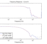
Figure 2: PD Plant Experimental and Model Frequency Response

Figure 2 shows the PD plant and the curve fit model frequency response. We have a 4thsuperscript4𝑡4^{th} order model which is used for control design and also a 10thsuperscript10𝑡10^{th} order model which will be used in a later section. We will design a Iterative learning control to better the performance of the inner loop controller. As can be seen from the model frequency response (Fig. 2) this system has a low bandwidth since the phase drops quite sharply (100osuperscript100𝑜100^{o} by 200 Hz).

Refer to caption

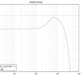
Figure 3: Stability Condition |Qu(z,z1)αQe(z,z1)G(z1)G(z)|<1subscriptsubscript𝑄𝑢𝑧superscript𝑧1𝛼subscript𝑄𝑒𝑧superscript𝑧1superscript𝐺superscript𝑧1superscript𝐺𝑧1\left|Q_{u}(z,z^{-1})-\alpha Q_{e}(z,z^{-1})G^{-}(z^{-1})G^{-}(z)\right|_{\infty}<1

Refer to caption


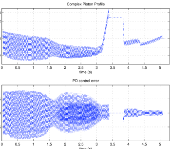
Figure 4: Complex Tool Profile (top) with PD Tracking Error (bottom)

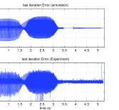
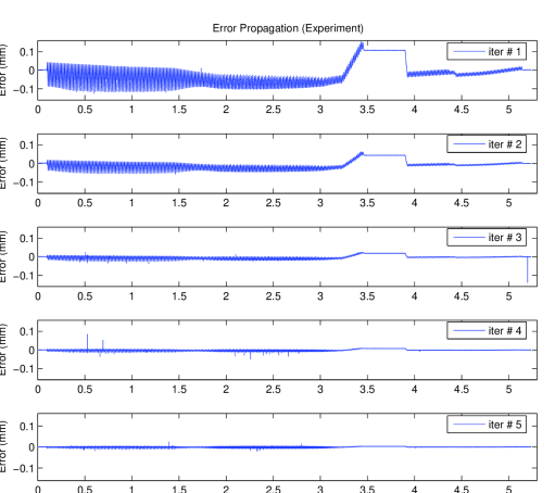
The top plot of Fig. 4 shows the complex profile as a function of time. What is shown is the depth of cut that the tool tip has to achieve. The command profile has periodic content between t=1s𝑡1𝑠t=1s and t=4s𝑡4𝑠t=4s reflecting oval cross-section and flat regions between t=3.5s𝑡3.5𝑠t=3.5s and t=3.8s𝑡3.8𝑠t=3.8s reflecting round cross-section. The profile is complex in the sense that although it looks periodic, the magnitude and phase changes gradually making it hard to follow. Also phase compensation apriori based on the plant’s frequency response (Fig. 2) is not possible due to the above reason. The bottom plot of Fig. 4 shows the error for the PD plant. The PD plant is not able to track this profile due to significant phase lag in the frequencies contained in the reference. We choose learning gain α=0.75𝛼0.75\alpha=0.75 and zero phase low pass filters Qusubscript𝑄𝑢Q_{u}, Qesubscript𝑄𝑒Q_{e} of orders 16 and 32 respectively. Fig. 3 shows that the stability condition is met for this choice of learning matrices. We start the experiment with 𝐮0=0subscriptsuperscript𝐮00\mathbf{u}^{\prime}_{0}=0, 𝐞0=rsubscript𝐞0𝑟\mathbf{e}_{0}=r. Figure 5 shows the tracking error for the first five iterations. We see that the error decreases uniformly over the entire time axis. Fig. 6 shows the 10thsuperscript10𝑡10^{th} iteration tracking error achieved by the scheme. We also did a simulation with no model mismatch for comparison with the experimental results . The error is within an acceptable ±10μmplus-or-minus10𝜇𝑚\pm 10\mu m compared to ±100μmplus-or-minus100𝜇𝑚\pm 100\mu m achieved with the PD controlled plant (see bottom plot of Fig. 4).
Refer to caption

Figure 5: Error Propagation for First Five Iterations (Experiment)

Refer to caption

Figure 6: Final Iteration Error Simulation (top) and Experiment (bottom)

VIII-A Improvement over ZPETC Feedforward Control

Assuming the system was at rest 𝐞0=𝐫subscript𝐞0𝐫\mathbf{e}_{0}=\mathbf{r} and 𝐮0=0subscriptsuperscript𝐮00\mathbf{u}^{\prime}_{0}=0 we have

𝐮1=α(𝐆)T𝐫𝐮1=α(𝐆+)1(𝐆)T𝐫subscriptsuperscript𝐮1𝛼superscriptsuperscript𝐆𝑇𝐫subscript𝐮1𝛼superscriptsuperscript𝐆1superscriptsuperscript𝐆𝑇𝐫\mathbf{u}^{\prime}_{1}=\alpha(\mathbf{G}^{-})^{T}\mathbf{r}\Rightarrow\mathbf{u}_{1}=\alpha(\mathbf{G}^{+})^{-1}(\mathbf{G}^{-})^{T}\mathbf{r}

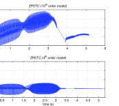
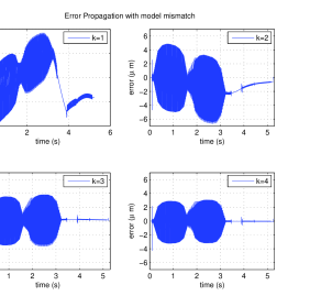
For the special choice of learning gain α=1𝛼1\alpha=1 this is equivalent to the celebrated zero phase error tracking control (ZPETC) [16]. Hence we infer that the first iteration of the prototype ILC (see section III-A) corresponds to stable inversion based feedforward compensation. It is well known that feedforward control such as the ZPETC is sensitive to plant model uncertainties. But the prototype ILC has an inherent cycle-to-cycle feedback which makes it “robust” in a limited sense. As reported in [18] zero phase ILC can be seen as repeated application of the feedforward control leading to better performance despite the presence of model uncertainties. Also the learning gain α𝛼\alpha is seldom set to the aggressive value of 111. Instead we use a lower gain and multiple iterations to derive the same effect as feedforward control in a ideal plant model situation. To verify the above claim, we did a simulation using a 4thsuperscript4𝑡4^{th} order model of the plant for the control design. Then we applied ZPETC feedforward control to a more accurate 10thsuperscript10𝑡10^{th} order model (see fig. 2). Figure 7 shows that the feedforward error is within ±30μmplus-or-minus30𝜇𝑚\pm 30\mu m when there is a model mismatch (top) as against ±5μmplus-or-minus5𝜇𝑚\pm 5\mu m when there is perfect model match (bottom). Figure 8 shows that we can improve upon the model mismatch error using the proposed modified repetitive ILC and bring it within the acceptable ±5μmplus-or-minus5𝜇𝑚\pm 5\mu m region in as few as four iterations.

Refer to caption


Figure 7: 10thsuperscript10𝑡10^{th} order model (top) 4thsuperscript4𝑡4^{th} order model (bottom) ZPETC error

Refer to caption

Figure 8: Error Propagation with model mismatch (Simulation)

IX Conclusions

We have introduced a noncausal ILC design based on zero-phase error compensation and filtering used in repetitive control design. The learning gains (matrices) are chosen carefully such that the resulting state transition matrix has a Symmetric Banded Toeplitz (SBT) structure. This special structure has been exploited to arrive at sufficient conditions for tracking error convergence in the frequency domain. Thus the ILC matrix design is translated to repetitive control loop shaping filter design in the frequency domain. For a special choice of learning matrix we have also derived a stronger monotonic convergence condition. Furthermore we have shown that under plant model mismatch the proposed scheme improves upon stable inversion based feedforward control. The proposed methodology has been successfully demonstrated on a fast tool servo system used in precision machining applications.

Appendix A

Theorem 1

The matrix 𝐀=𝐐uα𝐍T(𝐆)T𝐐e𝐆𝐍𝐀subscript𝐐𝑢𝛼superscript𝐍𝑇superscriptsuperscript𝐆𝑇subscript𝐐𝑒superscript𝐆𝐍\mathbf{A}=\mathbf{Q}_{u}-\alpha\mathbf{N}^{T}(\mathbf{G}^{-})^{T}\mathbf{Q}_{e}\mathbf{G}^{-}\mathbf{N} has a symmetric banded Toeplitz (SBT) structure

Proof:

Recall the definitions

𝐆i,jsubscriptsuperscript𝐆𝑖𝑗\displaystyle\mathbf{G}^{-}_{i,j} =\displaystyle= gij,0ijnusubscript𝑔𝑖𝑗0𝑖𝑗𝑛𝑢\displaystyle g_{i-j},\quad 0\leq i-j\leq nu
=\displaystyle= 0,otherwise0𝑜𝑡𝑒𝑟𝑤𝑖𝑠𝑒\displaystyle 0,\quad otherwise
(𝐐e)i,jsubscriptsubscript𝐐𝑒𝑖𝑗\displaystyle(\mathbf{Q}_{e})_{i,j} =\displaystyle= q|ij|e,|ij|nqsubscriptsuperscript𝑞𝑒𝑖𝑗𝑖𝑗𝑛𝑞\displaystyle q^{e}_{|i-j|},\quad|i-j|\leq nq
=\displaystyle= 0,otherwise0𝑜𝑡𝑒𝑟𝑤𝑖𝑠𝑒\displaystyle 0,\quad otherwise
𝐍i,jsubscript𝐍𝑖𝑗\displaystyle\mathbf{N}_{i,j} =\displaystyle= 1,1j=inun11𝑗𝑖𝑛𝑢𝑛\displaystyle 1,\quad 1\leq j=i-nu\leq n
=\displaystyle= 0,otherwise0𝑜𝑡𝑒𝑟𝑤𝑖𝑠𝑒\displaystyle 0,\quad otherwise

Hence we have the coefficients of (𝐐e𝐆)n+2nu,n+2nusubscriptsubscript𝐐𝑒superscript𝐆𝑛2𝑛𝑢𝑛2𝑛𝑢(\mathbf{Q}_{e}\mathbf{G}^{-})_{n+2nu,n+2nu} given by

bi,jsubscript𝑏𝑖𝑗\displaystyle b_{i,j} =\displaystyle= k=max(inq,j)min(i+nqe,j+nu,n+2nu)q|ik|egij,superscriptsubscript𝑘𝑚𝑎𝑥𝑖𝑛𝑞𝑗𝑚𝑖𝑛𝑖𝑛superscript𝑞𝑒𝑗𝑛𝑢𝑛2𝑛𝑢subscriptsuperscript𝑞𝑒𝑖𝑘subscript𝑔𝑖𝑗\displaystyle\sum_{k=max(i-nq,j)}^{min(i+nq^{e},j+nu,n+2nu)}q^{e}_{|i-k|}g_{i-j},
nqeijnqe+nu𝑛superscript𝑞𝑒𝑖𝑗𝑛superscript𝑞𝑒𝑛𝑢\displaystyle\quad\quad-nq^{e}\leq i-j\leq nq^{e}+nu
=\displaystyle= 0,otherwise0𝑜𝑡𝑒𝑟𝑤𝑖𝑠𝑒\displaystyle 0,\quad otherwise

The coefficients of (𝐐e𝐆𝐍)n+2nu,nsubscriptsubscript𝐐𝑒superscript𝐆𝐍𝑛2𝑛𝑢𝑛(\mathbf{Q}_{e}\mathbf{G}^{-}\mathbf{N})_{n+2nu,n} are given by

ci,jsubscript𝑐𝑖𝑗\displaystyle c_{i,j} =\displaystyle=
bi,j+nusubscript𝑏𝑖𝑗𝑛𝑢\displaystyle b_{i,j+nu} =\displaystyle= k=max(inqe,j+nu)min(i+nqe,j+2nu)q|ik|egkjnu,superscriptsubscript𝑘𝑚𝑎𝑥𝑖𝑛superscript𝑞𝑒𝑗𝑛𝑢𝑚𝑖𝑛𝑖𝑛superscript𝑞𝑒𝑗2𝑛𝑢subscriptsuperscript𝑞𝑒𝑖𝑘subscript𝑔𝑘𝑗𝑛𝑢\displaystyle\sum_{k=max(i-nq^{e},j+nu)}^{min(i+nq^{e},j+2nu)}q^{e}_{|i-k|}g_{k-j-nu},
nunqeijnqe+2nu𝑛𝑢𝑛superscript𝑞𝑒𝑖𝑗𝑛superscript𝑞𝑒2𝑛𝑢\displaystyle\quad\quad nu-nq^{e}\leq i-j\leq nq^{e}+2nu
=\displaystyle= 0,otherwise0𝑜𝑡𝑒𝑟𝑤𝑖𝑠𝑒\displaystyle 0,\quad otherwise

where we have used jnj+2nun+2nu𝑗𝑛𝑗2𝑛𝑢𝑛2𝑛𝑢j\leq n\Rightarrow j+2nu\leq n+2nu.
The coefficients of ((𝐆)T𝐐e𝐆𝐍)n+2nu,nsubscriptsuperscriptsuperscript𝐆𝑇subscript𝐐𝑒superscript𝐆𝐍𝑛2𝑛𝑢𝑛((\mathbf{G}^{-})^{T}\mathbf{Q}_{e}\mathbf{G}^{-}\mathbf{N})_{n+2nu,n} are given by

dl,jsubscript𝑑𝑙𝑗\displaystyle d_{l,j} =\displaystyle= i=1n+2nu(𝐆)i,lci,jsuperscriptsubscript𝑖1𝑛2𝑛𝑢subscriptsuperscript𝐆𝑖𝑙subscript𝑐𝑖𝑗\displaystyle\sum_{i=1}^{n+2nu}(\mathbf{G}^{-})_{i,l}c_{i,j}
=\displaystyle= i=max(l,j+nunqe)min(l+nu,j+2nu+nqe,n+2nu){gil\displaystyle\sum_{i=max(l,j+nu-nq^{e})}^{min(l+nu,j+2nu+nq^{e},n+2nu)}\{g_{i-l}
k=max(inqe,j+nu)min(i+nqe,j+2nu)q|ik|egkjnu},\displaystyle\sum_{k=max(i-nq^{e},j+nu)}^{min(i+nq^{e},j+2nu)}q^{e}_{|i-k|}g_{k-j-nu}\},
nqeljnqe+2nu𝑛superscript𝑞𝑒𝑙𝑗𝑛superscript𝑞𝑒2𝑛𝑢\displaystyle\quad\quad-nq^{e}\leq l-j\leq nq^{e}+2nu
=\displaystyle= 0,otherwise0𝑜𝑡𝑒𝑟𝑤𝑖𝑠𝑒\displaystyle 0,\quad otherwise

The coefficients of (𝐍T(𝐆)T𝐐e𝐆𝐍)n,nsubscriptsuperscript𝐍𝑇superscriptsuperscript𝐆𝑇subscript𝐐𝑒superscript𝐆𝐍𝑛𝑛(\mathbf{N}^{T}(\mathbf{G}^{-})^{T}\mathbf{Q}_{e}\mathbf{G}^{-}\mathbf{N})_{n,n} are given by

el,jsubscript𝑒𝑙𝑗\displaystyle e_{l,j} =\displaystyle=
dl+nu,jsubscript𝑑𝑙𝑛𝑢𝑗\displaystyle d_{l+nu,j} =\displaystyle= i=max(l+nu,j+nunqe)min(l+2nu,j+2nu+nqe){gilnu\displaystyle\sum_{i=max(l+nu,j+nu-nq^{e})}^{min(l+2nu,j+2nu+nq^{e})}\{g_{i-l-nu}
k=max(inqe,j+nu)min(i+nqe,j+2nu)q|ik|egkjnu},\displaystyle\sum_{k=max(i-nq^{e},j+nu)}^{min(i+nq^{e},j+2nu)}q^{e}_{|i-k|}g_{k-j-nu}\},
|lj|nqe+nu𝑙𝑗𝑛superscript𝑞𝑒𝑛𝑢\displaystyle\quad\quad|l-j|\leq nq^{e}+nu
=\displaystyle= 0,otherwise0𝑜𝑡𝑒𝑟𝑤𝑖𝑠𝑒\displaystyle 0,\quad otherwise

where we have used lnl+2nun+2nu𝑙𝑛𝑙2𝑛𝑢𝑛2𝑛𝑢l\leq n\Rightarrow l+2nu\leq n+2nu.
We do a change of variables i=inusuperscript𝑖𝑖𝑛𝑢i^{\prime}=i-nu and k=knusuperscript𝑘𝑘𝑛𝑢k^{\prime}=k-nu to get

el,jsubscript𝑒𝑙𝑗\displaystyle e_{l,j} =\displaystyle= i=max(l,jnqe)min(l+nu,j+nu+nqe){gil\displaystyle\sum_{i^{\prime}=max(l,j-nq^{e})}^{min(l+nu,j+nu+nq^{e})}\{g_{i^{\prime}-l}
k=max(inqe,j)min(i+nqe,j+nu)q|ik|egkj},\displaystyle\sum_{k^{\prime}=max(i^{\prime}-nq^{e},j)}^{min(i^{\prime}+nq^{e},j+nu)}q^{e}_{|i^{\prime}-k^{\prime}|}g_{k^{\prime}-j}\},
|lj|nqe+nu𝑙𝑗𝑛superscript𝑞𝑒𝑛𝑢\displaystyle\quad\quad|l-j|\leq nq^{e}+nu
=\displaystyle= 0,otherwise0𝑜𝑡𝑒𝑟𝑤𝑖𝑠𝑒\displaystyle 0,\quad otherwise

We readily see that

el+1,j+1subscript𝑒𝑙1𝑗1\displaystyle e_{l+1,j+1} =\displaystyle= i=max(l+1,j+1nqe)min(l+1+nu,j+1+nu+nqe){gil1\displaystyle\sum_{i^{\prime}=max(l+1,j+1-nq^{e})}^{min(l+1+nu,j+1+nu+nq^{e})}\{g_{i^{\prime}-l-1}
k=max(inqe,j+1)min(i+nqe,j+1+nu)q|ik|egkj1}\displaystyle\sum_{k^{\prime}=max(i^{\prime}-nq^{e},j+1)}^{min(i^{\prime}+nq^{e},j+1+nu)}q^{e}_{|i^{\prime}-k^{\prime}|}g_{k^{\prime}-j-1}\}
=\displaystyle= i=max(l,jnqe)min(l+nu,j+nu+nqe){gil\displaystyle\sum_{i=max(l,j-nq^{e})}^{min(l+nu,j+nu+nq^{e})}\{g_{i-l}
k=max(inqe,j)min(i+nqe,j+nu)q|ik|egkj}\displaystyle\sum_{k=max(i-nq^{e},j)}^{min(i+nq^{e},j+nu)}q^{e}_{|i-k|}g_{k-j}\}
=\displaystyle= el,jsubscript𝑒𝑙𝑗\displaystyle e_{l,j}

by doing a change of variable i=i1𝑖superscript𝑖1i=i^{\prime}-1 and k=k1𝑘superscript𝑘1k=k^{\prime}-1. Hence 𝐍T(𝐆)T𝐐e𝐆𝐍superscript𝐍𝑇superscriptsuperscript𝐆𝑇subscript𝐐𝑒superscript𝐆𝐍\mathbf{N}^{T}(\mathbf{G}^{-})^{T}\mathbf{Q}_{e}\mathbf{G}^{-}\mathbf{N} (which is symmetric by definition) is a SBT matrix. Since 𝐐usubscript𝐐𝑢\mathbf{Q}_{u} is by definition a SBT matrix, it follows that 𝐀𝐀\mathbf{A} is also a SBT matrix. ∎

Appendix B

Entries of the state transition matrix A -
When nqu>nqe+nu𝑛superscript𝑞𝑢𝑛superscript𝑞𝑒𝑛𝑢nq^{u}>nq^{e}+nu the coefficients of 𝐀𝐀\mathbf{A} are given by

fl,jsubscript𝑓𝑙𝑗\displaystyle f_{l,j} =\displaystyle= q|lj|uαi=max(l,jnqe)min(l+nu,j+nu+nqe){gil\displaystyle q^{u}_{|l-j|}-\alpha\sum_{i^{\prime}=max(l,j-nq^{e})}^{min(l+nu,j+nu+nq^{e})}\{g_{i^{\prime}-l}
k=max(inqe,j)min(i+nqe,j+nu)q|ik|gkj},\displaystyle\sum_{k^{\prime}=max(i^{\prime}-nq^{e},j)}^{min(i^{\prime}+nq^{e},j+nu)}q_{|i^{\prime}-k^{\prime}|}g_{k^{\prime}-j}\},
|lj|nqe+nu𝑙𝑗𝑛superscript𝑞𝑒𝑛𝑢\displaystyle\quad\quad|l-j|\leq nq^{e}+nu
=\displaystyle= q|lj|u,nqe+nu<|lj|nqusubscriptsuperscript𝑞𝑢𝑙𝑗𝑛superscript𝑞𝑒𝑛𝑢𝑙𝑗𝑛superscript𝑞𝑢\displaystyle q^{u}_{|l-j|},\quad nq^{e}+nu<|l-j|\leq nq^{u}
=\displaystyle= 0,otherwise0𝑜𝑡𝑒𝑟𝑤𝑖𝑠𝑒\displaystyle 0,\quad otherwise

When nqunqe+nu𝑛superscript𝑞𝑢𝑛superscript𝑞𝑒𝑛𝑢nq^{u}\leq nq^{e}+nu the coefficients of 𝐀𝐀\mathbf{A} are given by

fl,jsubscript𝑓𝑙𝑗\displaystyle f_{l,j} =\displaystyle= q|lj|uαi=max(l,jnqe)min(l+nu,j+nu+nqe){gil\displaystyle q^{u}_{|l-j|}-\alpha\sum_{i^{\prime}=max(l,j-nq^{e})}^{min(l+nu,j+nu+nq^{e})}\{g_{i^{\prime}-l}
k=max(inqe,j)min(i+nqe,j+nu)q|ik|gkj},\displaystyle\sum_{k^{\prime}=max(i^{\prime}-nq^{e},j)}^{min(i^{\prime}+nq^{e},j+nu)}q_{|i^{\prime}-k^{\prime}|}g_{k^{\prime}-j}\},
|lj|nqu𝑙𝑗𝑛superscript𝑞𝑢\displaystyle\quad\quad|l-j|\leq nq^{u}
=\displaystyle= αi=max(l,jnqe)min(l+nu,j+nu+nqe){gil\displaystyle-\alpha\sum_{i^{\prime}=max(l,j-nq^{e})}^{min(l+nu,j+nu+nq^{e})}\{g_{i^{\prime}-l}
k=max(inqe,j)min(i+nqe,j+nu)q|ik|gkj},\displaystyle\sum_{k^{\prime}=max(i^{\prime}-nq^{e},j)}^{min(i^{\prime}+nq^{e},j+nu)}q_{|i^{\prime}-k^{\prime}|}g_{k^{\prime}-j}\},
nqu<|lj|nqe+nu𝑛superscript𝑞𝑢𝑙𝑗𝑛superscript𝑞𝑒𝑛𝑢\displaystyle\quad\quad nq^{u}<|l-j|\leq nq^{e}+nu
=\displaystyle= 0,otherwise0𝑜𝑡𝑒𝑟𝑤𝑖𝑠𝑒\displaystyle 0,\quad otherwise

We get the entries in section V from the first row of the matrix

ak=f1,k+1,0krformulae-sequencesubscript𝑎𝑘subscript𝑓1𝑘10𝑘𝑟a_{k}=f_{1,k+1},\quad 0\leq k\leq r

where r=max(nqu,nqe+nu)𝑟𝑚𝑎𝑥𝑛superscript𝑞𝑢𝑛superscript𝑞𝑒𝑛𝑢r=max(nq^{u},nq^{e}+nu)

References

  • [1] S. Arimoto, S. Kawamura, and F. Miyazaki, “Bettering operation of robots by learning,” J. of Robotic Systems, vol. 1, no. 2, pp. 123–140, 1984.
  • [2] K. L. Moore, Iterative Learning Control for Deterministic Systems, ser. Advances in Industrial Control.   Springer-Verlag, 1993.
  • [3] Z. Bien and J.-X. Xu, Iterative Learning Control - Analysis, Design, Integration and Applications.   Boston, MA: Kluwer Academic Publishers, 1998.
  • [4] K. L. Moore, “Iterative learning control: A expository overview,” Applied and Computational Controls, Signal Processing and Circuits, vol. 1, no. 1, 1998.
  • [5] H.-S. Ahn, Y. Chen, and K. L. Moore, “Iterative learning control: Brief survey and categorization,” IEEE Trans. systems, man and cybernetics-part c: applications and reviews, vol. 37, no. 6, pp. 1099–1121, 2007.
  • [6] K. L. Moore, M. Dahleh, and S. Bhattacharyya, “Iterative learning for trajectory control,” in Proc. IEEE Conf. Decision and Control, Tampa, FL, Dec 1989, pp. 860–865.
  • [7] J. B. Edwards and D. H. Owens, Stability Analysis for Linear Repetitive Processes, ser. Lecture Notes on Control and Information Sciences.   NJ: Springer-Verlag, 1992.
  • [8] N. Amann, D. H. Owens, E. Rogers, and A. Wahl, “An hsubscripth_{\infty} approach to linear iterative learning control design,” Int. J. Adaptive Control and Signal Processing, vol. 10, pp. 767–781, 1996.
  • [9] D. Gorinevsky, “Loop-shaping for iterative learning control of batch processes,” IEEE Control Systems Mag., vol. 22, no. 6, pp. 55–65, Dec 2002.
  • [10] M. M. Norlöf and S. Gunnarsson, “Time and frequency domain convergence properties in iterative learning control,” Int. J. Control, vol. 75, no. 14, pp. 1114–1126, 2002.
  • [11] K. L. Moore and Y. Chen, “On the monotonic convergence of high-order iterative learning updating laws,” in Proc. IFAC Congress, Barcelona, Spain, July 2002.
  • [12] J. Hätönen, K. L. Moore, and D. H. Owens, “An algebraic approach to iterative learning control,” in Proc. IEEE Int. Symposium on Intelligent Control, Vancouver, Canada, 2002, pp. 37–42.
  • [13] K. L. Moore and Y. Chen, “A seperative high-order framework for monotonic convergent iterative learning controller design,” in Proc. American Control Conf., Denver, CO, June 2003, pp. 3644–3649.
  • [14] M. Norlöf, “Comparative study on first and second order ilc - frequency domain analysis and experiments,” in Proc. IEEE Conf. Decision and Control, Sydney, Australia, Dec 2000, pp. 3415–3420.
  • [15] J.-X. Xu and Y. Tan, “On the convergence speed of a class of higher-order ilc schemes,” in Proc. IEEE Conf. Decision and Control, Orlando, FL, Dec 2001, pp. 4932–4937.
  • [16] M. Tomizuka, “Zero phase error tracking algorithm for digital control,” J. Dynamic Systems, Measurement and Control, vol. 109, no. 1, pp. 87–92, Mar 1985.
  • [17] R. W. Longman, “Iterative learning control and repetitive control for engineering practise,” Int. J. Control, vol. 73, no. 10, pp. 930–954, 2000.
  • [18] H. Elci, R. W. Longman, M. Q. Phan, J.-N. Juang, and R. Ugoletti, “Simple learning control made practical by zero-phase filtering: Applications to robotics,” IEEE Trans. Circuits and Systems, vol. 49, no. 6, pp. 753–767, June 2002.
  • [19] S. Songschon and R. W. Longman, “Comparison of the stability boundary and the frequency response stability condition in learning and repetitive control,” Int. J. Appl. Math. Comput. Sci, vol. 13, no. 2, pp. 169–177, 2003.
  • [20] J.-X. Xu and R. Yan, “On repetitive learning control for periodic tracking tasks,” IEEE Trans. Automatic Control, vol. 51, no. 11, pp. 1842–1848, 2006.
  • [21] D. D. Roover, O. H. Bosgra, and M. Steinbuch, “Internal-model-based design of repetitive and iterative learning controllers for linear multivariable systems,” Int. J. Control, vol. 73, no. 10, pp. 914–929, 2000.
  • [22] Y. Chen, K. L. Moore, J. Yu, and T. Zhang, “Iterative learning control and repetitive control in hard disk drive industry - a tutorial,” in Proc. IEEE Conf. Decision and Control, San Diego, CA, Dec 2006, pp. 1–15.
  • [23] H. Elci, R. W. Longman, M. Q. Phan, J.-N. Juang, and R. Ugoletti, “Automated learning control through model updating for precision motion control,” Adaptive Structures and Composite Materials: Analysis and Application, vol. 45, pp. 299–314, 1994.
  • [24] N. Amann, D. Owens, and E. Rogers, “Predictive optimal iterative learning control,” Int. J. Control, vol. 69, no. 2, pp. 203–226, 1998.
  • [25] M. H. Verwoerd, G. Meinsma, and T. J. de Vries, “On the use of noncausal lti operators in iterative learning control,” in Proc. IEEE Conf. Decision and Control, Las Vegas, NV, Dec 2002, pp. 3362–3366.
  • [26] M. H. Verwoerd, “Iterative learning control - a critical review,” Ph.D. dissertation, University of Twente, Netherlands, 2005. [Online]. Available: http://www.ce.utwente.nl/rtweb/publications/2005/pdf-files/101CE2005_Verwoerd.pdf
  • [27] Y. Wu, Q. Zou, and C. Su, “A current cycle feedback iterative learning control approach for afm imaging,” IEEE Trans. Nanotechnology, vol. 8, no. 4, pp. 515–527, 2009.
  • [28] K. K. Leang and S. Devasia, “Iterative feedforward compensation of hysteresis in piezo positioners,” in Proc. IEEE Conf. Decision and Control, Maui, Hawaii, Dec 2003, pp. 2626–2631.
  • [29] S. Tien, Q. Zou, and S. Devasia, “Iterative control of dynamics-coupling effects in piezo-actuator for high-speed afm operation,” IEEE Trans. Contr. Syst. Technol.,, vol. 13, no. 6, pp. 921–931, 2005.
  • [30] K. Krishnamoorthy, C. Y. Lin, and T.-C. Tsao, “Design and control of a dual stage fast tool servo for precision machining,” in Proc. IEEE Conf. Control Applications, Taipei, Taiwan, 2004, pp. 742–747.
  • [31] M. Phan and R. Longman, “A mathematical theory of learning control for linear discrete multivariable systems,” in Proc. AIAA/AAS Astrodynamics Conf., Minneapolis, MN, Aug 1988, pp. 740–746.
  • [32] R. M. Gray, “Toeplitz and circulant matrices: A review,” Foundations and Trends in Communications and Information Theory, vol. 2, no. 3, pp. 155–239, 2006. [Online]. Available: http://www-ee.stanford.edu/similar-to\simgray/toeplitz.html
  • [33] K. L. Moore, “An observation about monotonic convergence in discrete-time, p-type iterative learning control,” in Proc. IEEE Int. Symposium on Intelligent Control, Mexico, Sep 2001, pp. 45–49.
  • [34] M. Tomizuka, T.-C. Tsao, and K.-K. Chew, “Analysis and synthesis of discrete-time repetitive controllers,” J. Dynamic Systems, Measurement and Control, vol. 111, pp. 353–358, Sep 1989.
  • [35] K.-K. Chew and M. Tomizuka, “Digital control of repetitive errors in disk drive systems,” IEEE Control Systems Mag., pp. 16–20, Jan 1990.
  • [36] B. A. Francis and W. M. Wonham, “The internal model principle for linear multivariable regulators,” Applied Math., Opt.,, vol. 2, pp. 170–194, 1975.
  • [37] D. Bini and V. Pan, “Efficient algorithms for the evaluation of the eigenvalues of (block) banded toeplitz matrices,” Mathematics of Computation, vol. 50, no. 182, pp. 431–448, Apr 1988.
  • [38] P. Arbenz, “Computing eigenvalues of banded symmetric toeplitz matrices,” SIAM J. Sci. and Stat. Comput., vol. 12, no. 4, pp. 743–754, July 1991.
  • [39] G. D. Smith, Numerical Solution of Partial Differential Equations, ser. Oxford Applied Mathematics and Computing Science, 2, Ed.   Oxford, U.K.: Clarendon Press.
[Uncaptioned image] Krishnamoorthy Kalyanam received the B.Tech. degree in mechanical engineering from the Indian Institute of Technology Madras, Chennai, India in 2000, and the M.S. and Ph.D. degrees in mechanical engineering from The University of California at Los Angeles, in 2003 and 2005, respectively. In 2005 he joined the General Electric Company’s Global Research Center, Bengaluru, India as a Research Engineer. He is currently a National Research Council Research Associate working at the Air Force Research Lab, Wright-Patterson Air Force Base, Ohio. His current research interests include cooperative control of multivehicle systems, adaptive and learning control.
[Uncaptioned image] Tsu-Chin Tsao (S’86-M’88-SM’09) received the B.S. degree in engineering from National Taiwan University, Taipei, Taiwan, in 1981, and the M.S. and Ph.D. degrees in mechanical engineering from The University of California at Berkeley, in 1984 and 1988, respectively. In 1999, he joined the faculty of the University of California at Los Angeles, where he is currently a Professor with the Department of Mechanical and Aerospace Engineering. For 11 years, he was with the faculty of the Department of Mechanical and Industrial Engineering, The University of Illinois at Urbana-Champaign. His research interests include control systems and mechatronics. Prof. Tsao is a recipient of the ASME Journal of Dynamic Systems, Measurement, and Control Best Paper Award for papers published in the journal in 1994, the Outstanding Young Investigator Award from ASME Dynamic Systems and Control Division in 1997, and the Hugo S. Shuck Best Paper Award.