HATS-6b: A Warm Saturn Transiting an Early M Dwarf Star, and a Set of Empirical Relations for Characterizing K and M Dwarf Planet Hosts

Abstract

We report the discovery by the HATSouth survey of HATS-6b, an extrasolar planet transiting a V=$15.2$ mag, $i=13.7$ mag M1V star with a mass of $0.57$ $M_{\sun}$ and a radius of $0.57$ $R_{\sun}$. HATS-6b has a period of $P\approx 3.3253$ d, mass of $M_{p}\approx 0.32$ $M_{\rm J}$, radius of $R_{p}\approx 1.00$ $R_{\rm J}$, and zero-albedo equilibrium temperature of $T_{\rm eq}=712.8\pm 5.1$ K. HATS-6 is one of the lowest mass stars known to host a close-in gas giant planet, and its transits are among the deepest of any known transiting planet system. We discuss the follow-up opportunities afforded by this system, noting that despite the faintness of the host star, it is expected to have the highest $K$-band S/N transmission spectrum among known gas giant planets with $T_{\rm eq}<750$ K. In order to characterize the star we present a new set of empirical relations between the density, radius, mass, bolometric magnitude, and $V$, $J$, $H$ and $K$-band bolometric corrections for main sequence stars with $M<0.80$ $M_{\sun}$, or spectral types later than K5. These relations are calibrated using eclipsing binary components as well as members of resolved binary systems. We account for intrinsic scatter in the relations in a self-consistent manner. We show that from the transit-based stellar density alone it is possible to measure the mass and radius of a $\sim 0.6$ $M_{\sun}$ star to $\sim 7$% and $\sim 2$% precision, respectively. Incorporating additional information, such as the $V-K$ color, or an absolute magnitude, allows the precision to be improved by up to a factor of two.

1. Introduction

One of the goals in the study of exoplanetary systems is to determine how the properties of planets depend on the properties of their host stars. An important parameter in this respect is the host star mass. Results from both radial velocity and transit surveys indicate that the occurrence rate of gas giant planets is a steep function of stellar mass scaling approximately as $N\propto M_{\star}$ (Johnson et al., 2010) for main sequence stars of type M through F (smaller planets, on the other hand, appear to be more frequent around M dwarfs than around hotter stars, Howard et al., 2012). The low occurrence rate of these planets around M dwarfs, coupled with the fact that most surveys primarily target FGK dwarf stars, means that only one hot Jupiter has so far been discovered around an M0 dwarf (Kepler-45; Johnson et al., 2012), and only a handful of others have been found around very late K dwarf stars (WASP-80, Triaud et al., 2013b; WASP-43, Hellier et al., 2011; and HAT-P-54, Bakos et al., 2014, being the only three known transiting-hot-Jupiter-hosting K dwarfs with $M<0.65\,M_{\sun}$).

In addition to enabling the study of planetary properties as a function of stellar mass, finding planets around late-type stars has at least two other advantages. The small sizes of these stars coupled with their low luminosities means that a planet with a given radius and orbital period around a late-type star will produce deeper transits and have a cooler equilibrium temperature than if it were around a larger star. This makes planets around late-type stars attractive targets for carrying out detailed follow-up observations, such as atmospheric characterizations. A second, perhaps under appreciated, advantage of these stars is that they are remarkably simple in their bulk properties. Whereas, due to stellar evolution, the radius of a solar-metallicity, solar-mass star varies by $\sim 40\%$ over the 10 Gyr age of the Galactic disk, the radius of a $0.6$ $M_{\sun}$ star varies by less than $\sim 5$% over the same time-span. The parameters of low-mass stars follow tight main-sequence relations, enabling high-precision measurements of their properties from only a single (or a few) observable(s). The precision of the stellar parameters feeds directly into the precision of the planetary parameters, so that in principle planets around low-mass stars may be characterized with higher precision than those around higher mass stars.

Here we present the discovery of a transiting, short-period, gas-giant planet around an M1 dwarf star. This planet, HATS-6b, was discovered by the HATSouth survey, a global network of fully-automated wide-field photometric instruments searching for transiting planets (Bakos et al., 2013). HATSouth uses larger-diameter optics than other similar projects allowing an enhanced sensitivity to faint K and M dwarfs.

We also present a new set of empirical relations to use in characterizing the properties of transiting planet host stars with $M<0.80$ $M_{\sun}$. While there has been much discussion in the literature of the apparent discrepancy between observations and various theoretical models for these stars (e.g., Torres & Ribas, 2002; Ribas, 2003; Torres, 2013; Zhou et al., 2014, and references therein), the growing set of well-characterized low-mass stars has revealed that, as expected, these stars do follow tight main sequence relations. We show that from the bulk density of the star alone, which is determined from the transit light curve and RV observations, it is possible to measure the mass and radius of a $\sim 0.6$ $M_{\sun}$ star to $\sim 7\%$ and $\sim 2\%$ precision, respectively. Incorporating additional information, such as the $V-K$ color, or an absolute magnitude, allows the precision to be improved by a factor of two.

The layout of the paper is as follows. In Section 2 we report the detection of the photometric signal and the follow-up spectroscopic and photometric observations of HATS-6. In Section 3 we describe the analysis of the data, beginning with ruling out false positive scenarios, continuing with our global modelling of the photometry and radial velocities, and finishing with the determination of the stellar parameters, and planetary parameters which depend on them, using both theoretical stellar models as well as the empirical relations which we derive here. Our findings are discussed in Section 4.

2. Observations

Figure 1.— Unbinned instrumental $r$-band light curve of HATS-6 folded with the period $P=3.3252725$ days resulting from the global fit described in Section 3. The solid line shows the best-fit transit model (see Section 3). In the lower panel we zoom-in on the transit; the dark filled points here show the light curve binned in phase using a bin-size of 0.002.

Figure 2.— Left: Unbinned follow-up transit light curves of HATS-6. The dates, filters and instruments used for each event are indicated. The light curves have been detrended using the EPD process. Curves after the first are shifted for clarity. Our best fit is shown by the solid lines. Right: Residuals from the fits in the same order as the curves at left. Additional follow-up light curves from GROND are shown in Figure 3.

Figure 3.— Unbinned instrumental Sloan $g$-, $r$-, $i$- and $z$-band transit light curves of HATS-6 obtained with GROND on the MPG 2.2 m on the night of UT 2014 March 6. The light curves have been detrended using the EPD process, and the best-fit is shown by the solid lines. Below each light curve we plot the residuals.

2.1. Photometric detection

Observations of a field containing HATS-6 (see Table 9 for identifying information) were carried out with the HS-2, HS-4 and HS-6 units of the HATSouth network (located at Las Campanas Observatory in Chile, the H.E.S.S. gamma-ray telescope site in Namibia, and Siding Spring Observatory in Australia, respectively; see Bakos et al., 2013 for a detailed description of the HATSouth network) between UT 2009-09-17 and UT 2010-09-10. A total 5695, 5544 and 88 images included in our final trend and outlier-filtered light curves were obtained with HS-2, HS-4 and HS-6, respectively. Observations were made through a Sloan $r$ filter, using an exposure time of $240$ s and a median cadence of $293$ s (see also Table 1).

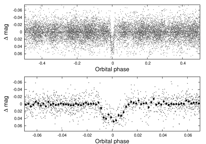
The data were reduced to trend-filtered light curves following Bakos et al. (2013). We apply two empirical trend filtering techniques to the data. The first is to decorrelate the light curves against a set of measured parameters which vary from image to image, including the $X$ and $Y$ sub-pixel coordinates of the star, three parameters describing the shape of the image point spread function, the hour angle of the observations, the zenith distance, and the sky background near the target. We refer to this filtering as External Parameter Decorrelation (EPD; Bakos et al., 2010). The second filtering technique is to use the Trend Filtering Algorithm (TFA) due to Kovács et al. (2005). In this method we select a list of $\sim 800$ template light curves uniformly distributed in position across the field, and coming from stars with a broad range of magnitudes. We then fit the EPD-filtered light curve for HATS-6 as a linear combination of these $\sim 800$ templates, and subtract the fit from the observations. The filtered light curve for HATS-6 has a point-to-point RMS of 0.02 mag and is dominated by noise from the background sky. Transits were identified in the resulting HATSouth light curve of HATS-6 using the Box Least Squares (BLS; Kovács et al., 2002) algorithm. Figure 1 shows the phase-folded HATSouth light curve of HATS-6 together with our best-fit transit model, while the photometric measurements are provided in Table 2.2.

We searched the residual HATSouth light curve for additional transit signals using BLS but found no significant detection. We also searched for continuous quasi-periodic variability using both the Discrete Fourier Transform (Kurtz, 1985) and the Discrete Autocorrelation Function (Edelson & Krolik, 1988). We find a possible signal in the pre-TFA light curve with a period of $P=35.1$ d and an S/N, measured in the power spectrum, of 12.3. This signal is not seen in the Autocorrelation Function, nor is it seen in the light curve after processing with TFA. While potentially due to stellar rotation, this may also be time-correlated noise. We therefore do not claim a measurement of the photometric rotation period for this star.

2.2. Photometric follow-up

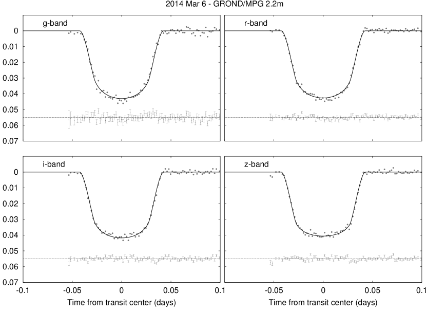
In order to confirm the transit signal, and determine the parameters of the system with better accuracy, we carried out follow-up photometric observations of HATS-6 using the 0.3 m Perth Exoplanet Survey Telescope (PEST), the CTIO 0.9 m, telescopes in the LCOGT 1 m network (Brown et al., 2013), and GROND on the MPG 2.2 m (Greiner et al., 2008). Key aspects of these observations, including the dates of the observations, the number of images obtained, the cadence, filter used, and the precision of the resulting HATS-6 light curves, as measured from the RMS of the residuals from our best-fit model, are summarized in Table 1. The light curves are plotted in Figures 2 and 3, while the measurements are provided in Table 2.2. Details regarding the PEST instrument, our observational procedure, as well as our reduction and photometry methods can be found in Zhou et al. (2014); see Penev et al. (2013) and Mohler-Fischer et al. (2013) for similar information regarding the GROND observations. Because this is the first time we have used the CTIO 0.9 m and the LCOGT 1 m network, we describe our use of these facilities in more detail below.

On the nights of 2012 Sep. 3 and 2013 Oct. 27, we performed photometric observations of HATS-6 using the CTIO 0.9 m telescope, which has a CCD with a $13\farcm 6\times 13\farcm 6$ field of view. On the first night we used a Gunn $z^{\prime}$ filter and on the latter one a Kron-Cousins $R_{C}$ filter. We defocused the telescope in order to broaden the point spread function. Images from both nights were calibrated (bias subtracted and flat fielded) with custom Python routines. A fringing effect was seen in the images taken during our full moon night in $z$-band. However, images taken with the $R_{C}$ filter did not show fringing. Therefore, we also took 53 empty field regions with the Gunn $z^{\prime}$ filter during our 2012 Sep. CTIO run. We combined these images and subtracted the sky background, and then scaled the combined image to match, and remove, the additive fringing effect seen in the science images. To reduce the calibrated images to light curves, we chose a reference image and calculated the shift of all images with respect to the reference image. From the reference image we extracted the position of the stars. Following Deeg & Doyle (2001), the time series photometry was generated from these observations using optimized aperture photometry that maximizes the signal-to-noise ratio (S/N) for each star. For all images in one night we used three fixed apertures and choose these to be much larger than the typical point spread function in order to minimize the impact of the time-variable point spread functions. The resulting light curves of HATS-6 have precisions of $4.7$ mmag and $3.7$ mmag on the first and second nights, respectively.

Observations of HATS-6 were carried out using the LCOGT 1 m network on the UT nights of 2013-11-23 and 2013-12-07. We used one of the three telescopes installed at the South African Astronomical Observatory (SAAO) on the night of 2013-11-23, and one of the telescopes at CTIO on the night of 2013-12-07. In both cases we used the SBIG STX-16803 4K$\times$4K imagers with which the telescopes were initially deployed. These imagers provided a $16\arcmin\times 16\arcmin$ field of view with a pixel scale of $0\farcs 23$. We used a Pan-STARSS $z_{S}$ filter for the first night, and a Sloan $i^{\prime}$ filter for the second night. Other details regarding the instrumentation can be found in Brown et al. (2013). Calibrated science images were provided by the LCOGT 1 m pipeline. We performed astrometry and aperture photometry using tools from the FITSH package (Pál, 2012) on these images following methods that we have previously applied to observations from the Faulkes Telescopes, North and South, as well as to observations from Keplercam on the Fred Lawrence Whipple Observatory 1.2 m telescope. This procedure is described in Bakos et al. (2010).

Table 1 Summary of photometric observations

Facility	Date(s)	Number of Images	Cadence (s)	Filter	Precision (mmag)
HS-2	2009 Sep–2010 Sep	5695	295	$r$	21.3
HS-4	2009 Sep–2010 Sep	5544	293	$r$	21.0
HS-6	2010 Aug–2010 Sep	88	296	$r$	18.6
CTIO 0.9 m	2012 Sep 03	34	297	$z$	4.7
PEST 0.3 m	2013 Feb 17	58	205	$R$	6.1
PEST 0.3 m	2013 Feb 27	53	131	$R$	5.6
PEST 0.3 m	2013 Mar 29	24	261	$R$	4.8
CTIO 0.9 m	2013 Oct 27	99	181	$R_{C}$	3.7
LCOGT 1 m	2013 Nov 23	48	76	$z$	4.2
LCOGT 1 m	2013 Dec 07	149	74	$i$	3.8
GROND/MPG 2.2 m	2014 Mar 06	95	155	$g$	1.8
GROND/MPG 2.2 m	2014 Mar 06	95	155	$r$	1.1
GROND/MPG 2.2 m	2014 Mar 06	95	155	$i$	1.1
GROND/MPG 2.2 m	2014 Mar 06	95	155	$z$	1.1

Table 2Differential photometry of HATS-6

BJD	Mag	$\sigma_{\rm Mag}$	Mag(orig)	Filter	Instrument
(2 400 000$+$)
$55185.60957$	$-0.00387$	$0.01084$	$\cdots$	$r$	HS
$55145.70640$	$-0.07475$	$0.03251$	$\cdots$	$r$	HS
$55095.82750$	$-0.01258$	$0.01255$	$\cdots$	$r$	HS
$55275.39406$	$0.02245$	$0.01229$	$\cdots$	$r$	HS
$55195.58763$	$-0.00021$	$0.01587$	$\cdots$	$r$	HS
$55182.28728$	$0.00324$	$0.01174$	$\cdots$	$r$	HS
$55145.70968$	$-0.00768$	$0.02964$	$\cdots$	$r$	HS
$55185.61296$	$0.02073$	$0.01078$	$\cdots$	$r$	HS
$55095.83089$	$-0.02280$	$0.01379$	$\cdots$	$r$	HS
$55105.80688$	$-0.02863$	$0.02168$	$\cdots$	$r$	HS

[-1.5ex]

Note. — This table is available in a machine-readable form in the online journal. A portion is shown here for guidance regarding its form and content. The data are also available on the HATSouth website at http://www.hatsouth.org.

2.3. Spectroscopy

Table 3 summarizes the follow-up spectroscopic observations which we obtained for HATS-6.

2.3.1 Reconnaissance Spectroscopy

Initial reconnaissance spectroscopic observations of HATS-6 were carried out using the Wide Field Spectrograph (WiFeS; Dopita et al., 2007) on the ANU 2.3 m telescope at SSO together with the Echelle spectrograph on the du Pont 2.5 m telescope at LCO. The ANU 2.3 m data were reduced and analyzed following Bayliss et al. (2013), while for the du Pont data we used the pipeline we have previously developed (Jordán et al., 2014) to analyze data from the Coralie and FEROS spectrographs, adapted for the different spectral format of the instrument. A single WiFeS spectrum was obtained with a resolution of $R\equiv\lambda/\Delta\lambda=3000$ to use in measuring the effective temperature, surface gravity, and metallicity of the star, while four observations were obtained at a resolution of $R=7000$ to check for RV variations with amplitude $\gtrsim 5$ $\rm km\,s^{-1}$ that would indicate that the transiting companion is of stellar mass. The two du Pont spectra each had a resolution of $R=40000$ covering a wavelength range of $3700$–$7000$ Å, and were used to measure the effective temperature, gravity, metallicity, projected rotation velocity and radial velocity of the star. Like the WiFeS spectra, the RV precision of the du Pont observations ($\sim 500$ $\rm m\,s^{-1}$) is not high enough to detect velocity variations due to a planet, but is sufficient to rule out stellar-mass companions.

Our analysis of the $R=3000$ WiFeS spectrum indicated an effective temperature of $T_{\rm eff\star}=3600\pm 300$ K, while the du Pont spectra yielded $T_{\rm eff\star}=3700\pm 100$ K. This effective temperature corresponds to a spectral type of M1 (Rajpurohit et al., 2013). The spectrum shows clear TiO absorption bands, and is consistent with an M1V spectral classification. This spectrum also shows that HATS-6 is a quiet M-dwarf, with no evidence of emission in the H$\alpha$ or Ca II H and K line cores. Additional indications that HATS-6 is a quiet star are the lack of any obvious star-spot crossing events in the photometric follow-up light curves (Figures 2 and 3), and the lack of large-amplitude photometric variability in the HATSouth light curve. The WiFeS spectrum also indicated a dwarf-like surface gravity ($\log{g_{\star}}=3.9\pm 0.3$; c.g.s. units) and a possibly sub-solar metallicity ($\rm[Fe/H]$$=-1.0\pm 0.5$), while our analysis of the du Pont spectra yielded a somewhat lower surface gravity ($\log{g_{\star}}=3.2\pm 0.5$) and metallicity ($\rm[Fe/H]$$=-1.5\pm 0.5$) and a moderately high rotation velocity ($v\sin{i}=7.5\pm 2.0$ $\rm km\,s^{-1}$). The analysis, however, relies on synthetic templates (MARCS models in the case of WiFeS and models from Coelho et al., 2005 in the case of du Pont) which are known to be unreliable for M type stars. This means that systematic errors in the determined parameters are most likely greater than the estimated uncertainties (especially when $T_{\rm eff\star}$, $\log{g_{\star}}$ and $\rm[Fe/H]$, which are strongly correlated with each other, are all allowed to vary in fitting the spectra). As an example of this, note that based on the Dartmouth single stellar evolution models (Dotter et al., 2008) the minimum surface gravity realized for a $T_{\rm eff\star}=3700$ K dwarf star within 13.8 Gyr is $\log{g_{\star}}=4.73$ which is significantly higher than the values determined from the spectroscopic modelling (the only evolved single stars that reach $T_{\rm eff\star}=3700$ K have $\log{g_{\star}}\lesssim 2$). We therefore do not consider the $\log{g_{\star}}$  $\rm[Fe/H]$, or $v\sin{i}$ measurements from this analysis to be reliable. More reliable estimate of $T_{\rm eff\star}$ and $\rm[Fe/H]$ are presented in the next section.

2.3.2 Confirmation Spectroscopy

In order to confirm HATS-6 as a transiting planet system through a detection of the RV orbital variation we obtained high-resolution spectra with three facilities capable of achieving $\sim 10$ $\rm m\,s^{-1}$ or better RV precision. These are the FEROS spectrograph (Kaufer & Pasquini, 1998) on the MPG 2.2 m telescope at La Silla Observatory (LSO), the Planet Finder Spectrograph (PFS; Crane et al., 2010) on the Magellan Clay 6.5 m telescope at LCO, and the High Accuracy Radial Velocity Planet Searcher (HARPS; Mayor et al., 2003) spectrograph on the ESO 3.6 m telescope at LSO. Figure 4 shows the phased RV measurements and bisector spans from these observations, together with our best-fit orbit, while Table 2.3.2 lists the individual measurements.

A total of 8 $R=48000$ spectra were obtained with FEROS between 2013 Mar 24 and 2013 May 13. Details on the FEROS spectra as used by HATSouth have been provided by Mohler-Fischer et al. (2013). For the observations reported we did not follow the reduction procedure described previously, and instead reduced the data using an adapted version of the pipeline described by Jordán et al. (2014). This pipeline, which utilizes cross-correlation against binary templates, was originally developed for the CORALIE spectrograph on the Euler 1.2 m telescope at LSO. We found that applying this pipeline to FEROS data yields a precision of $\sim$8 $\rm m\,s^{-1}$ for RV standard stars, which is significantly better than the $\gtrsim 20$ $\rm m\,s^{-1}$ precision previously achieved for this instrument. This will be described in additional detail in a separate paper (Brahm et al. in preparation).

The PFS observations consisted of an I₂-free template spectrum obtained on the night of UT 2013 Nov 8, and 7 observations taken through an I₂ cell obtained between 2013 Nov 7 and 16. Observations were carried out with a $0\farcs 5\times 2\farcs 5$ slit, using $2\times 2$ binning and slow read-out mode. The spectra were reduced to RVs in the bary-centric frame of the solar system following the method of Butler et al. (1996). We computed bisector spans in a manner similar to that used by Torres et al. (2007) to calculate bisector spans for Keck/HIRES data. The presence of the I₂ cell restricts the spectral range over which the bisector spans may be computed. Whereas in Torres et al. (2007), and previous studies using Keck/HIRES data, the bisector span analysis was done on the bluest spectral orders which are free of I₂ absorption, the faintness and extreme red color of HATS-6 makes the signal blueward of $5000$ Å too low to be used for a bisector analysis. We therefore use five orders covering the spectral range $6200$ Å to $6540$ Å. The limited spectral range reduces the precision of the bisector spans. In fact we find that the bisector spans calculated from the MPG 2.2 m/FEROS data have lower scatter than those from Magellan/PFS. Nonetheless there is no significant trend in the bisector spans, nor is there any evidence for more than one stellar component in the Magellan/PFS cross-correlation functions.

We used our I₂-free template spectrum from PFS to measure $T_{\rm eff}$ and [Fe/H] for HATS-6 following the method of Neves et al. (2014). We made use of the Python routines referenced in that paper to perform this analysis, after modifying it for the spectral range of PFS (we verified that the code reproduces the temperature and metallicity of the two HARPS spectra supplied with the routines, when applied to the restricted spectral range). We find $T_{\rm eff\star}=3770\pm 100{}$ K and [Fe/H]$=0.200\pm 0.091{}$, where the errors are determined from Table 6 of Neves et al. (2014) scaling by $\sqrt{N_{\rm all}/N_{\rm used}}$ where $N_{\rm all}$ is the number of spectral lines used by Neves et al. (2014), and $N_{\rm used}$ is the number of lines within the PFS spectral range.

The HARPS observations consisted of three exposures taken on the nights of UT 2013 Dec 7–9. We used an exposure time of 1200 s on the first night and 1800 s on the following two nights. Observations were carried out in the “object+sky” mode (due to the faintness of the target, contamination from scattered moonlight is substantial), and reduced to RVs using the facility Data Reduction Software (DRS) together with a K star spectral mask (at present this is the coolest facility mask available). The spectra have a resolution of $R=115000$ covering a range of 378 nm–691 nm.

In practice, due to the faintness of HATS-6 and the low mass of the planet HATS-6b, the orbital variation is detected with significance only from the PFS data. We include the data from HARPS and FEROS in our RV model (Section 3.2) for completeness, and to ensure that the fit accounts for all data, including non-detections.

Table 3 Summary of spectroscopic observations

Telescope/Instrument	Date Range	Number of Observations	Resolution	Observing Mode
ANU 2.3 m/WiFeS	2012 May 13	1	3000	Recon Spectral Type
ANU 2.3 m/WiFeS	2012 Aug 6–Oct 24	4	7000	Recon RVs
du Pont 2.5 m/Echelle	2012 Oct 25–26	2	30000	Recon RVs/Spectral Type
Magellan Clay 6.5 m/PFS	2013 Nov 7–16	7	100000	High Precision RVs
MPG 2.2 m/FEROS	2013 Mar 24–May 11	8	48000	High Precision RVs
ESO 3.6 m/HARPS	2013 Dec 7–10	31	115000	High Precision RVs

Figure 4.— Top panel: High-precision RV measurements for HATS-6 from Magellan/PFS (dark filled circles), MPG 2.2 m/FEROS (open triangles), and ESO 3.6 m/HARPS (stars), together with our best-fit circular orbit model. Zero phase corresponds to the time of mid-transit. The center-of-mass velocity has been subtracted. The orbital fit is primarily constrained by the PFS observations. Second panel: Velocity $O\!-\!C$ residuals from the best-fit model. The error bars for each instrument include the jitter which is varied in the fit. Third panel: Bisector spans (BS), with the mean value subtracted. Note the different vertical scales of the panels.

Table 4 Relative radial velocities and bisector span measurements of HATS-6.

3. Analysis

3.1. Excluding blend scenarios

In order to rule out the possibility that HATS-6 is not a planetary system, but is instead a blend between an eclipsing binary star and another source, we carried out a blend analysis similar to that done in Hartman et al. (2012), with a difference being that in this case we use the Dartmouth (Dotter et al., 2008) stellar evolution models to calculate the properties of simulated blended systems. We find that although there exist blend models involving a eclipsing binary blended with a brighter foreground M dwarf which match the light curves and absolute photometry, in all such cases both the foreground source and the primary in the background binary have an apparent magnitude difference $|\Delta V|<1$ mag, so that cross-correlation functions (CCFs) computed from the PFS, FEROS and HARPS spectra would show obvious secondary peaks and RV variations greater than $1$ $\rm km\,s^{-1}$. The simulated CCFs are grossly inconsistent with the observed CCFs, so we conclude that this is not a blended eclipsing binary system, and is instead a transiting planet system.

As is often the case we cannot exclude the possibility that HATS-6 is an unresolved binary system with one component having a transiting planet. High resolution imaging would provide constraints on any such wide binary companions. For the analysis presented here we assume that this is an isolated star. If future observations reveal that this is a binary system, corrections to the planet mass and radius would increase their values from those presented in this paper.

3.2. Global Fit of Light Curves and RV Measurements

In order to determine the physical parameters of the HATS-6 system we carried out an analysis similar to that described in Bakos et al. (2010); Penev et al. (2013). All light curves (HATSouth data and follow-up data) and RV measurements are simultaneously fitted using a Mandel & Agol (2002) transit light curve model and a Keplerian RV orbit.

The light curve model is extended using a model for instrumental variations such that the total model can be expressed as:

$$m_{k,i} = m_{k,0}+\Delta m(t_{i};T_{0},T_{N_{t}},\zeta/R_{\star},R_{p}/R_{\star},b,a_{{\rm LD},k},b_{{\rm LD},k})$$ (1)

$$+\sum_{j=1}^{N_{{\rm EPD},k}}c_{{\rm EPD},k,j}x_{k,j,i}+\sum_{j=1}^{N_{\rm TFA}}c_{{\rm TFA},j}y_{k,j,i}$$

where $m_{k,i}$ is the measured magnitude to be modeled for observation $i$ of light curve $k$; $m_{k,0}$ is the zero-point magnitude for light curve $k$ (which is a free parameter in the model); $\Delta m(t_{i};T_{0},T_{N_{t}},\zeta/R_{\star},R_{p}/R_{\star},b,a_{{\rm LD},k},b_{{\rm LD},k})$ is the physical Mandel & Agol (2002) model evaluated at time $t_{i}$ and parameterized by initial and final transit epochs $T_{0}$ and $T_{N_{t}}$ (the period is then given by $(T_{N_{t}}-T_{0})/N_{t}$), reciprocal of the half duration of the transit $\zeta/R_{\star}$, ratio of the planetary and stellar radii $R_{p}/R_{\star}$, normalized impact parameter $b$, and quadratic limb darkening coefficients $a_{{\rm LD},k}$ and $b_{{\rm LD},k}$ appropriate for the filter of light curve $k$ (except for $a_{{\rm LD},k}$ and $b_{{\rm LD},k}$, which are fixed using the tabulations of Claret (2004), these parameters are varied in the fit); there are $N_{{\rm EPD},k}$ EPD parameters applied to light curve $k$ with $c_{{\rm EPD},k,j}$ being the free coefficient fitted for EPD parameter series $j$ applied to light curve $k$, and $x_{k,j,i}$ being the value of EPD parameter series $j$ at observation $i$ for light curve $k$; and there are $N_{\rm TFA}$ TFA templates used to fit the light curve, with $c_{{\rm TFA},j}$ being the free coefficient fitted for template $j$ and $y_{k,j,i}$ being the value of template $j$ at observation $i$ for light curve $k$. For the HATSouth light curve we do not include the EPD and TFA terms in the fit, and instead model the light curve that was pre-processed through these filtering routines without accounting for the transits. In this case we also include an instrumental blending factor (varied in the fit) which scales the depth of the Mandel & Agol (2002) model applied to the HATSouth light curve by a factor between 0 and 1 (assuming a uniform prior between these limits) to account for both blending from nearby stars as well as the artificial dilution of signals due to the filtering.

For the RV model we allow an independent RV zero-point, and an independent RV jitter for each of the three instruments used. The jitter is a term added in quadrature to the formal RV uncertainties for each instrument and is varied in the fit following Hartman et al. (2012).

We use a Differential Evolution Markov-Chain Monte Carlo (DEMCMC) procedure (ter Braak, 2006; Eastman et al., 2013) to explore the fitness of the model over parameter space and produce a chain of parameters drawn from the posterior distribution. This chain is then used to estimate the most likely value (taken as the median value over the chain) together with the 68.3% ($1\sigma$) confidence interval for each of the physical parameters.

The fit is performed both allowing the eccentricity to vary, and fixing it to zero. We find that without additional constraints, the free-eccentricity model strongly prefers a non-zero eccentricity of $e=0.404\pm 0.058{}$. This is entirely due to the PFS velocities which closely follow such an eccentric orbit with a near-zero jitter for the PFS RVs of $0.1\pm 5.6{}$ $\rm m\,s^{-1}$. When the eccentricity is fixed to zero, on the other hand, the PFS RVs are consistent with a circular orbit, but in this case require a jitter of $26\pm 14{}$ $\rm m\,s^{-1}$. Due to the faintness of HATS-6 in the optical band-pass, and consequent sky contamination, such a high “jitter” is not unreasonable, and may simply reflect an underestimation of the formal RV uncertainties. As we discuss below, the stellar parameters inferred for the high eccentricity solution are inconsistent with the spectroscopic parameters and broad-band photometric colors of the star. When the photometric observations are directly folded into our light curve and RV modelling, as we discuss in Section 3.3.2, the preferred eccentricity is consistent with zero ($e=0.053\pm 0.060$).

3.3. Determining the Physical Parameters of the Star and Planet

To determine the mass and radius of the transiting planet from the physical parameters measured above requires knowledge of the stellar mass and radius. For a non-binary star such as HATS-6 these parameters are not easy to measure directly and instead must be inferred by comparing other measurable parameters, such as the surface temperature and bulk stellar density, with theoretical stellar evolution models (requiring the metallicity, a color indicator, and a luminosity indicator to identify a unique stellar model), or with empirical relations calibrated using binary stars. We considered both methods, discussed in turn below.

3.3.1 Dartmouth Models

Because the star is a cool dwarf we make use of the Dartmouth stellar evolution models (Dotter et al., 2008) which appear to provide the best match to M dwarf and late K dwarf stars (e.g. Feiden et al., 2011; Sandquist et al., 2013). We also use the effective temperature and metallicity measured from the PFS I₂-free template spectrum.

We use the results from our DEMCMC analysis of the light curve and radial velocity data (Section 3.2) together with the Dartmouth isochrones to determine the stellar parameters. For each density measurement in the posterior parameter chain we associate T_eff and $\rm[Fe/H]$ measurements drawn from Gaussian distributions. We look up a matching stellar model from the Dartmouth isochrones, interpolating between the tabulated models, and append the set of stellar parameters associated with this model to the corresponding link in the posterior parameter chain. Other planetary parameters, such as the mass and radius, which depend on the stellar parameters are then calculated for each link in the chain.

Figure 5 compares the measured $T_{\rm eff}$ and $\rho_{\star}$ values for HATS-6 to the interpolated [Fe/H]$=0.20$ Dartmouth isochrones. We also compare the $V-K$ and $\rho_{\star}$ values to these same isochrones. For reference we show seven transiting-planet-hosting stars with $T_{\rm eff\star}$, $V-K$, $\rho_{\star}$ and $M_{\star}$ similar to that of HATS-6. These are listed as well in Table 3.3.2. At fixed $T_{\rm eff}$ or $V-K$ the models predict $\rho_{\star}$ values that are slightly lower than those seen amongst the transit hosts. This suggests that using $V-K$ as an input in constraining the mass of the star through the Dartmouth models may lead to a slightly overestimated stellar mass (lower densities yield higher masses). For comparison we also show the relations derived from the empirical relations discussed below. The empirical relations appear to provide a better match to the stars shown in Figure 5.

Figure 5.— Model isochrones (dashed lines) from Dotter et al. (2008) for the spectroscopically determined metallicity of HATS-6 and ages of 1 to 13 Gyr in 1 Gyr steps (showing $\rho_{\star}$ vs $T_{\rm eff}$ at top, $\rho_{\star}$ vs $V-K$ in the middle, and $M_{\star}$ vs $V-K$ at the bottom). The measured values of $T_{\rm eff}$, $V-K$, and $\rho_{\star}$ for HATS-6, and the value of $M_{\star}$ inferred from comparison to the stellar models, are shown using the large filled circles together with their 1$\sigma$ and 2$\sigma$ confidence ellipsoids. The open triangles show other transiting planet host stars with measured $T_{\rm eff}$, $V-K$, $\rho_{\star}$ and $M_{\star}$ values similar to HATS-6. Near the K/M spectral type boundary ($V-K\sim 4$) the models predict somewhat lower densities for a given $V-K$ or $T_{\rm eff}$ than are seen among transit hosts (Table 3.3.2). For comparison we also show the relations derived from our empirical model (dotted lines; Section 3.3.2). In the top panel we show the three dotted lines are the median relation, and the $1\sigma$ lower and upper bounds. In the bottom two panels the lower dotted line is the median relation, while the upper dotted line is the $1\sigma$ upper bound. The $1\sigma$ lower bound from the empirical model lies just outside the range of these plots (below the bottom left corner in each case). The empirical models appear to be more consistent with the transiting planet hosts than the theoretical models, but also cover a broader range of parameter space than seen among the transit hosts.

Figure 6.— Top: Empirical relation between stellar density and radius (equation 2, with parameters given in Table 7). The solid line shows the best-fit relation with $dR=0$, the dashed lines show the expected $1\sigma$ spread for this relation allowing $dR$ to be drawn from a Gaussian distribution with standard deviation $S_{R}$. The points show the eclipsing binary components from Table 3.3.2 used to fit this relation. Middle: Same as top, here we show the empirical relation between stellar density and mass. Bottom: Same as top, here we show the empirical relation between stellar mass and bolometric magnitude. On the right-hand panels we show the fractional residuals from the best-fit models, the short-dashed (blue) lines show the expected relations from the Dartmouth stellar models for an age of 4.5 Gyr and solar metallicity, while the longer dashed (red) lines show the expected $1\sigma$ spread from the empirical model. The solar-metallicity 4.5 Gyr Dartmouth models predict systematically larger radii at fixed density, and brighter bolometric magnitudes at fixed mass, than observed in the eclipsing binary sample. The empirical models provide a good fit to these data, by design.

As noted in Section 3.2 when we allow the eccentricity to vary in the fit the PFS data pull the model toward a high eccentricity solution ($e=0.404\pm 0.058$) which also yields a high stellar density of $14.8\pm 2.9$ $\rm g\,cm^{-3}$. The combination of the high stellar density, hot effective temperature ($T_{\rm eff\star}=3770\pm 100$ K) and high metallicity ([Fe/H]$=0.200\pm 0.091$) cannot be matched by the Dartmouth isochrones. If we instead use $V-K$ as the temperature indicator and draw metallicities from the Haywood (2001) solar neighborhood metallicity distribution we find that only very low metallicity models ($[Fe/H]=-0.63\pm 0.07$) match the observations. Such a metallicity is at odds with the spectroscopic measurement. Moreover, taking the parameters from the eccentric model, and assuming $Q_{P}=10^{6}$ the circularization timescale (e.g. Adams & Laughlin, 2006) is only $342\pm 35$ Myr. No planets with $t_{\rm circ}<1$ Gyr have been found with eccentricities greater than 0.1 (e.g. see Fig. 12 of Bakos et al., 2012), making it unlikely that HATS-6b has such a high eccentricity.

3.3.2 Empirical Relations

As an alternative method to determine the stellar parameters, and to better understand the degree of systematic errors in these parameters, we also develop a set of empirical relations between stellar density, which is directly measured for a transiting planet system, and other stellar parameters. Such relations have been developed and employed in transiting exoplanet studies previously (Torres et al., 2010; Enoch et al., 2010; Southworth, 2011). The Torres et al. (2010) and Enoch et al. (2010) relations only considered stars with $M>0.6$ $M_{\sun}$, making them inapplicable in this case. The Southworth (2011) relations consider stars over the range $0.2\,M_{\sun}<M<3.0\,M_{\sun}$. They present two relations, one for mass as a function of temperature, density and metallicity, the other for radius as a function of temperature, density and metallicity. Fitting these as two independent functions ignores the fact that density, mass, and radius must satisfy the relation $M=\frac{4}{3}\pi R^{3}\rho$. Moreover, one should not expect the scaling of mass and radius with metallicity or temperature to be independent of stellar mass over such a broad range in mass. And, since metallicity is available for only very few M dwarf eclipsing binaries, the fit performed by Southworth (2011) effectively imposes the metallicity scaling for A through G stars on the M dwarfs. We therefore consider it worthwhile to revisit these relations for K and M dwarf stars.

Johnson et al. (2011) and Johnson et al. (2012) have also developed empirical relations for characterizing M dwarf planet hosts, applying them to the characterization of LHS 6343 AB and Kepler-45, respectively. Our approach is similar to theirs in that we make use of relations between mass and absolute magnitudes based on data from Delfosse et al. (2000), and we also consider the empirical mass–radius relation based on eclipsing binaries, however we differ in the sample of eclipsing binaries that we consider, and we adopt a different parameterization of the problem. Moreover, while Johnson et al. (2012) use several empirical relations which were independently fit using different data sets, our approach is to self-consistently determine all of the relations through a joint analysis of the available data. We discuss this comparison in more detail below.

Figure 7.— Top: Empirical relation between effective temperature and the bolometric correction in $V$-band (upper left), $J$-band (upper right), $H$-band (lower left) and $K$-band (lower right). In each case the solid line is the median relation, while the dashed lines show the $1\sigma$ confidence region about the median relation. The points in this plot correspond to stars in Table 6 with T_eff and $M_{\rm bol}$ for each star determined as part of the empirical model fitting procedure. Because T_eff and $M_{\rm bol}$ are not directly observed parameters for these stars, but are rather determined through the modelling, and largely constrained by the stellar mass, which is observed, the data appear to follow the model very closely. This should not be taken as validation of the model (see instead Figure 8), rather the purpose of showing these plots is to demonstrate the form of the bolometric correction, its uncertainty, as well as the range of temperatures over which the model is constrained.

Figure 8.— Top: Same as Figure 7, here we show the empirical relation between stellar mass and the absolute magnitudes in the $V$, $J$, $H$ and $K$ bands. The residuals from these fits are shown in Figure 9.

We look for the following relations: (1) $\rho_{\star}\rightarrow R_{\star}$ (which also defines a $\rho_{\star}\rightarrow M_{\star}$ relation), (2) $M_{\star}\rightarrow M_{\rm bol}$, (which together with relation 1 also defines a relation between $T_{\rm eff\star}$ and the other parameters) (3) $T_{\rm eff\star}\rightarrow M_{\rm bol}-M_{V}$, (4) $T_{\rm eff\star}\rightarrow M_{\rm bol}-M_{J}$, (5) $T_{\rm eff\star}\rightarrow M_{\rm bol}-M_{H}$, (6) $T_{\rm eff\star}\rightarrow M_{\rm bol}-M_{K}$. The motivation for choosing this particular formulation is that $\rho_{\star}$ is typically a well-measured parameter for transiting planet systems, and the relation between $\rho_{\star}$ and $R_{\star}$ is tighter than for other relations involving $\rho_{\star}$. The other relations are then based on physical dependencies (bolometric magnitude depends primarily on stellar mass, with age and metallicity being secondary factors, and bolometric corrections depend primarily on effective temperature, with metallicity being a secondary factor). These relations are parameterized as follows:

$$lR=\left(\begin{array}[]{c}a_{\rho,0}\\ a_{\rho,1}\\ a_{\rho,2}\\ a_{\rho,3}\end{array}\right)^{T}\left(\begin{array}[]{cccc}0.131674&-0.605624&0.739127&-0.263765\\ -0.494952&0.614479&0.437886&-0.430922\\ -0.765425&-0.291096&0.099548&0.565224\\ 0.389626&0.413398&0.502032&0.652117\end{array}\right)\left(\begin{array}[]{c}1\\ l\rho\\ l\rho^{2}\\ l\rho^{3}\end{array}\right)+dlR$$ (2)

$$M_{\rm bol}=\left(\begin{array}[]{c}b_{m,0}\\ b_{m,1}\\ b_{m,2}\\ b_{m,3}\end{array}\right)^{T}\left(\begin{array}[]{cccc}-0.042114&-0.349391&-0.787638&-0.505746\\ 0.170316&0.723492&0.095153&-0.662192\\ -0.309788&-0.505183&0.591641&-0.546610\\ -0.934479&0.315080&-0.143296&0.083309\end{array}\right)\left(\begin{array}[]{c}1\\ lM\\ lM^{2}\\ lM^{3}\end{array}\right)+dM_{\rm bol}$$ (3)

$$BC_{\lambda}=\left(\begin{array}[]{c}c_{\lambda,0}\\ c_{\lambda,1}\\ c_{\lambda,2}\end{array}\right)^{T}\left(\begin{array}[]{ccc}0.871464&-0.485768&0.067675\\ 0.484681&0.831841&-0.270418\\ 0.075065&0.268461&0.960361\end{array}\right)\left(\begin{array}[]{c}1\\ lT\\ lT^{2}\end{array}\right)$$ (4)

where $lR=\log_{10}(R)$, $l\rho=\log_{10}(\rho)$, $lM=\log_{10}(M)$, $lT=\log_{10}(T_{\rm eff})$ are the logarithms of the stellar radius in solar units, density in cgs units, mass in solar units and temperature in Kelvin, respectively. The sets of coefficients in the vectors to the left of the matrices (e.g., $a_{\rho,0}$, $a_{\rho,1}$, etc.; optimal values are given in Table 7) are varied in the fit, and the matrices are chosen to minimize correlations between these parameters. The matrices are determined by initially fitting the relations using simple polynomials (i.e. we replace the matrices in the relations above with the identity matrix), and then performing a Principal Component Analysis on the resulting Markov Chains to determine the transformation to a linearly uncorrelated set of parameters. These matrices are held fixed in a subsequent fit where we determine the optimized values of the parameters $a_{\rho,0}$, $a_{\rho,1}$, etc. (see below for more discussion of the fitting procedure). The term $\lambda$ is either $V$, $J$, $H$ or $K$. To allow for intrinsic scatter in the relations, the terms $dlR$ and $dM_{\rm bol}$ represent real deviations in the radius or bolometric magnitude from the model. Such deviations are expected due to additional parameters, such as the metallicity or age, which are not included in this model. Every star has its own value of $dlR$ and $dM_{\rm bol}$, assumed to be drawn from Gaussian distributions with standard deviations of $S_{R}$ and $S_{Mbol}$, respectively. The following auxiliary relations are also used to relate the stellar density to the mass, the bolometric magnitude and radius to the effective temperature, and the bolometric magnitude and bolometric correction to the absolute magnitude in a given filter ($M_{\lambda}$):

$$lM = l\rho-0.14968+3lR(l\rho)$$ (5)

$$lT = (42.227-5lR-M_{bol})/10$$ (6)

$$M_{\lambda} = M_{\rm bol}+BC_{\lambda}.$$ (7)

Figure 9.— Same as Figure 8, here we show residuals from the median empirical relation. The short-dash (blue) lines show the relation from the 4.5 Gyr, Solar metallicity Dartmouth models, while the long-dash (red) lines show the expected $1\sigma$ spread of the empirical model.

Figure 10.— Top: Comparison of the precision with which stellar mass (left) and stellar radius (right) may be measured using either $\rho_{\star}$, $M_{V}$, $M_{K}$, or $V-K$ as an observed parameter. For each observable we step through a range of values determining the median stellar mass (radius) and its standard deviation using the empirical relations given in equations 2 through 4. We find that $M_{K}$ is the highest precision stellar mass indicator, allowing a precision that varies between $\sim 3$% and $6$%, whereas $\rho_{\star}$ is the highest precision stellar radius indicator, allowing a precision of $\sim 2$% over the range $0.2\,R_{\sun}<R<0.9\,R_{\sun}$. Bottom: Comparison of the precision with which stellar mass (left) and stellar radius (right) may be measured using the combinations of parameters indicated in the figure. Combining the density with an absolute magnitude indicator allows for a mass precision between 2.5% and 4.5%, and a radius precision between $\sim 1$% and $\sim 2$%.

The stars that we use in the fit are listed in Tables 3.3.2 and 6. The eclipsing binaries are compiled from tables in Zhou et al. (2014), Torres et al. (2010), and Nefs et al. (2013), and include non-pre-main-sequence stars with $M_{\star}<0.85\,M_{\sun}$ and with $M_{\star}$ and $R_{\star}$ measured to better than 5% accuracy. The upper mass limit corresponds roughly to the mass for which stars older than the pre-main-sequence phase, and with $-0.5<[Fe/H]<0.5$, will have $\log g>4.4$ throughout the $\sim 10$ Gyr age of the Galactic disk. Stars below this mass show tight correlations between the density and the mass, radius and luminosity. Because individual broad-band photometric magnitudes are not available for most of the eclipsing binary components, we use resolved binaries for which masses and component magnitudes are available to constrain relations (3) through (6) above. Most of these stars are taken from the compilation by Delfosse et al. (2000), with a few objects from the list of Torres et al. (2010) to extend into the late K dwarf regime.

To fit the above relations we use a likelihood function of the form:

$$\ln L = -\frac{1}{2}\sum_{i=1}^{N_{\star}}\left(\frac{lR(l\rho_{i})-lR_{{\rm obs},i}}{\sigma_{lR,i}}\right)^{2}$$

$$-\frac{1}{2}\sum_{i=1}^{N_{\star}}\left(\frac{lM(l\rho_{i})-lM_{{\rm obs},i}}{\sigma_{lM,i}}\right)^{2}$$

$$-\frac{1}{2}\sum_{i=1}^{N_{\star}}\left(\frac{lT(lR(l\rho_{i}),M_{\rm bol}(lM(l\rho_{i})))-lT_{{\rm obs},i}}{\sigma_{lT,i}}\right)^{2}$$

$$-\frac{1}{2}\sum_{\lambda}\sum_{i=1}^{N_{\star}}\left(\frac{M_{\rm bol}(lM(l\rho_{i}))+BC_{\lambda}(lT(lR(l\rho_{i}),M_{\rm bol}(lM(l\rho_{i}))))-M_{\lambda,obs,i}}{\sigma_{\lambda,i}}\right)^{2}$$

$$-\frac{1}{2}\sum_{i=1}^{N_{\star}}\left(\ln(S_{R}^{2})+\left(\frac{dlR_{i}}{S_{R}}\right)^{2}\right)$$

$$-\frac{1}{2}\sum_{i=1}^{N_{\star}}\left(\ln(S_{Mbol}^{2})+\left(\frac{dM_{{\rm bol},i}}{S_{Mbol}}\right)^{2}\right)$$

where the sum on $\lambda$ is over the four filters $V$, $J$, $H$ and $K$, and for each star we exclude terms from the sums if the relevant measurement ($lR_{\rm obs}$, $lM_{\rm obs}$, $lT_{\rm obs}$, $M_{V,obs}$, $M_{J,obs}$, $M_{H,obs}$, or $M_{K,obs}$) is not available. Here $l\rho_{i}$, $dlR_{i}$, and $dM_{{\rm bol},i}$ are free parameters for each star $i$, and the other free parameters are $S_{R}$, $S_{Mbol}$, and the coefficients in equations 2–4. We use the DEMCMC procedure to explore this likelihood function. Table 7 provides the values for the best-fit model together with their approximate $1\sigma$ (uncorrelated) uncertainties.

Table 5 K and M Dwarf Binary Components Used to Fit Empirical Relations

Star	Mass	Radius	Teff	Reference
	($M_{\sun}$)	($R_{\sun}$)	(K)
1 RXS J154727.5+450803 A	$0.2576\pm 0.0085$	$0.2895\pm 0.0068$	$\ldots$	1
1 RXS J154727.5+450803 B	$0.2585\pm 0.0080$	$0.2895\pm 0.0068$	$\ldots$	1
ASA J011328–3821.1 A	$0.612\pm 0.03$	$0.596\pm 0.02$	$3750\pm 250$	2
CG Cyg B	$0.814\pm 0.013$	$0.838\pm 0.011$	$4720\pm 60$	3,4
CM Dra A	$0.2130\pm 0.0009$	$0.2534\pm 0.0019$	$3130\pm 70$	5
CM Dra B	$0.2141\pm 0.0010$	$0.2396\pm 0.0015$	$3120\pm 70$	5
CU Cnc A	$0.4333\pm 0.0017$	$0.4317\pm 0.0052$	$3160\pm 150$	6
CU Cnc B	$0.3980\pm 0.0014$	$0.3908\pm 0.0094$	$3130\pm 150$	6
GJ 3236 A	$0.376\pm 0.016$	$0.3795\pm 0.0084$	$3310\pm 110$	7
GJ 551	$0.123\pm 0.006$	$0.141\pm 0.007$	$3098\pm 56$	8,9,10
GU Boo A	$0.610\pm 0.006$	$0.627\pm 0.016$	$3920\pm 130$	11
GU Boo B	$0.600\pm 0.006$	$0.624\pm 0.016$	$3810\pm 130$	11
HATS550-016	$0.110^{+0.005}_{-0.006}$	$0.147^{+0.003}_{-0.004}$	$\ldots$	12
HATS551-021	$0.132^{+0.014}_{-0.005}$	$0.154^{+0.006}_{-0.008}$	$\ldots$	12
HD 195987 A	$0.844\pm 0.018$	$0.98\pm 0.04$	$5200\pm 100$	13
J1219-39 B	$0.091\pm 0.002$	$0.1174^{+0.0071}_{-0.0050}$	$\ldots$	14
Kepler-16 B	$0.20255^{+0.00066}_{-0.00065}$	$0.22623^{+0.00059}_{-0.00055}$	$\ldots$	15
KIC 1571511 B	$0.14136^{+0.0051}_{-0.0042}$	$0.17831^{+0.0013}_{-0.0016}$	$\ldots$	16
KOI-126 B	$0.2413\pm 0.0030$	$0.2543\pm 0.0014$	$\ldots$	17
KOI-126 C	$0.2127\pm 0.0026$	$0.2318\pm 0.0013$	$\ldots$	17
LSPM J1112+7626 A	$0.3946\pm 0.0023$	$0.3860\pm 0.0055$	$3060\pm 160$	18
LSPM J1112+7626 B	$0.2745\pm 0.0012$	$0.2978\pm 0.0049$	$2950\pm 160$	18
MG1-116309 A	$0.567\pm 0.002$	$0.552\pm 0.0085$	$3920\pm 80$	19
MG1-116309 B	$0.532\pm 0.002$	$0.532\pm 0.006$	$3810\pm 80$	19
MG1-1819499 A	$0.557\pm 0.001$	$0.569\pm 0.0022$	$3690\pm 80$	19
MG1-1819499 B	$0.535\pm 0.001$	$0.500\pm 0.0085$	$3610\pm 80$	19
MG1-2056316 A	$0.4690\pm 0.0021$	$0.441\pm 0.002$	$3460\pm 180$	19
MG1-2056316 B	$0.382\pm 0.001$	$0.374\pm 0.002$	$3320\pm 180$	19
MG1-506664 A	$0.584\pm 0.002$	$0.560\pm 0.0025$	$3730\pm 90$	19
MG1-506664 B	$0.544\pm 0.002$	$0.513\pm 0.0055$	$3610\pm 90$	19
MG1 646680A	$0.499\pm 0.002$	$0.457\pm 0.006$	$3730\pm 50$	19
MG1-646680 B	$0.443\pm 0.002$	$0.427\pm 0.006$	$3630\pm 50$	19
MG1-78457 B	$0.491\pm 0.002$	$0.471\pm 0.009$	$3270\pm 100$	19
NSVS 01031772 A	$0.5428\pm 0.0027$	$0.526\pm 0.0028$	$3615\pm 72$	20
NSVS 01031772 B	$0.4982\pm 0.0025$	$0.5087\pm 0.0031$	$3520\pm 30$	20
NSVS 6550671 A	$0.510\pm 0.02$	$0.550\pm 0.01$	$3730\pm 60$	21
T-Cyg1-01385 B	$0.43\pm 0.02$	$0.40\pm 0.02$	$\ldots$	22
UV Psc B	$0.7644\pm 0.0045$	$0.835\pm 0.018$	$4750\pm 80$	23
V568 Lyr B	$0.8273\pm 0.0042$	$0.7679\pm 0.0064$	$4900\pm 100$	24
WOCS 23009 B	$0.447\pm 0.011$	$0.4292\pm 0.0033$	$3620\pm 150$	25
WTS19b-2-01387 A	$0.498\pm 0.019$	$0.496\pm 0.013$	$3498\pm 100$	26
WTS19b-2-01387 B	$0.481\pm 0.017$	$0.479\pm 0.013$	$3436\pm 100$	26
YY Gem A	$0.599\pm 0.005$	$0.619\pm 0.006$	$3819\pm 98$	27
YY Gem B	$0.599\pm 0.005$	$0.619\pm 0.006$	$3819\pm 98$	27

References. — 1: Hartman et al. (2011); 2: Hełminiak et al. (2012); 3: Bedford et al. (1987); 4: Popper (1994); 5: Morales et al. (2009); 6: Ribas (2003); 7: Irwin et al. (2009); 8: Ségransan et al. (2003); 9: Valenti & Fischer (2005); 10: Demory et al. (2009); 11: López-Morales & Ribas (2005); 12: Zhou et al. (2014); 13: Torres et al. (2002); 14: Triaud et al. (2013a); 15: Doyle et al. (2011); 16: Ofir et al. (2012); 17: Carter et al. (2011); 18: Irwin et al. (2011); 19: Kraus et al. (2011); 20: Lopez-Morales et al. (2006); 21: Dimitrov & Kjurkchieva (2010); 22: Fernandez et al. (2009); 23: Popper (1997); 24: Grundahl et al. (2008); 25: Sandquist et al. (2013); 26: Birkby et al. (2012); 27: Torres & Ribas (2002)

Table 6 K and M Dwarf Stars with Absolute Magnitudes and Measured Masses Used in Fitting the Bolometric Corrections in the Empirical Stellar Model

Star	Mass	$M_{V}$	$M_{J}$	$M_{H}$	$M_{K}$
	($M_{\sun}$)	(mag)	(mag)	(mag)	(mag)
Gl 866 C	$0.0930\pm 0.0008$	$17.43\pm 0.40$	$\ldots$	$\ldots$	$\ldots$
Gl 65 B	$0.100\pm 0.010$	$15.87\pm 0.06$	$10.06\pm 0.05$	$9.45\pm 0.03$	$9.16\pm 0.07$
Gl 65 A	$0.102\pm 0.010$	$15.41\pm 0.05$	$9.68\pm 0.05$	$9.15\pm 0.03$	$8.76\pm 0.07$
Gl 234 B	$0.1034\pm 0.0035$	$16.16\pm 0.07$	$10.31\pm 0.25$	$9.56\pm 0.10$	$9.26\pm 0.04$
Gl 623 B	$0.1142\pm 0.0083$	$16.02\pm 0.11$	$10.47\pm 0.29$	$9.35\pm 0.05$	$9.33\pm 0.14$
Gl 866 B	$0.1145\pm 0.0012$	$15.64\pm 0.08$	$\ldots$	$9.29\pm 0.04$	$8.96\pm 0.04$
Gl 866 A	$0.1187\pm 0.0011$	$15.39\pm 0.07$	$\ldots$	$\ldots$	$\ldots$
Gl 791.2 B	$0.126\pm 0.003$	$16.64\pm 0.10$	$\ldots$	$\ldots$	$\ldots$
Gl 473 B	$0.131\pm 0.010$	$15.00\pm 0.07$	$9.57\pm 0.06$	$9.04\pm 0.07$	$8.84\pm 0.08$
Gl 473 A	$0.143\pm 0.011$	$15.01\pm 0.07$	$9.44\pm 0.06$	$8.84\pm 0.06$	$8.40\pm 0.06$
Gl 831 B	$0.1621\pm 0.0065$	$14.62\pm 0.08$	$\ldots$	$8.62\pm 0.05$	$8.36\pm 0.05$
Gl 860 B	$0.1762\pm 0.0066$	$13.46\pm 0.09$	$9.03\pm 0.08$	$8.40\pm 0.05$	$8.32\pm 0.07$
Gl 747 B	$0.1997\pm 0.0008$	$12.52\pm 0.06$	$\ldots$	$\ldots$	$7.63\pm 0.04$
Gl 234 A	$0.2027\pm 0.0106$	$13.07\pm 0.05$	$8.52\pm 0.06$	$7.93\pm 0.04$	$7.64\pm 0.04$
CMDra B	$0.2136\pm 0.0010$	$12.94\pm 0.10$	$\ldots$	$\ldots$	$\ldots$
Gl 747 A	$0.2137\pm 0.0009$	$12.30\pm 0.06$	$\ldots$	$\ldots$	$7.53\pm 0.04$
CMDra A	$0.2307\pm 0.0010$	$12.80\pm 0.10$	$\ldots$	$\ldots$	$\ldots$
Gl 860 A	$0.2711\pm 0.0100$	$11.76\pm 0.05$	$7.84\pm 0.04$	$7.26\pm 0.04$	$6.95\pm 0.04$
Gl 791.2 A	$0.286\pm 0.006$	$13.37\pm 0.03$	$\ldots$	$\ldots$	$\ldots$
Gl 831 A	$0.2913\pm 0.0125$	$12.52\pm 0.06$	$\ldots$	$7.36\pm 0.05$	$7.08\pm 0.05$
Gl 644 Bb	$0.3143\pm 0.0040$	$11.71\pm 0.10$	$\ldots$	$\ldots$	$\ldots$
Gl 623 A	$0.3432\pm 0.0301$	$10.74\pm 0.05$	$7.19\pm 0.04$	$6.70\pm 0.04$	$6.46\pm 0.04$
Gl 644 Ba	$0.3466\pm 0.0047$	$11.22\pm 0.10$	$\ldots$	$\ldots$	$\ldots$
Gl 661 B	$0.369\pm 0.035$	$11.15\pm 0.06$	$7.51\pm 0.04$	$7.02\pm 0.04$	$6.78\pm 0.05$
Gl 570 C	$0.3770\pm 0.0018$	$11.09\pm 0.17$	$7.40\pm 0.04$	$6.76\pm 0.04$	$6.57\pm 0.04$
Gl 661 A	$0.379\pm 0.035$	$11.10\pm 0.06$	$7.10\pm 0.05$	$6.56\pm 0.04$	$6.36\pm 0.05$
GJ 2069 Ab	$0.3987\pm 0.0007$	$12.57\pm 0.19$	$\ldots$	$\ldots$	$\ldots$
Gl 644 A	$0.4155\pm 0.0057$	$10.76\pm 0.06$	$\ldots$	$6.61\pm 0.05$	$6.35\pm 0.04$
GJ 2069 Aa	$0.4344\pm 0.0008$	$11.78\pm 0.18$	$\ldots$	$\ldots$	$\ldots$
Gl 570 B	$0.5656\pm 0.0029$	$9.45\pm 0.05$	$6.21\pm 0.03$	$5.61\pm 0.03$	$5.39\pm 0.03$
YYGem A	$0.6028\pm 0.0014$	$9.03\pm 0.12$	$\ldots$	$\ldots$	$\ldots$
YYGem B	$0.6069\pm 0.0014$	$9.38\pm 0.14$	$\ldots$	$\ldots$	$\ldots$
HD 195987 B	$0.6650\pm 0.0079$	$7.91\pm 0.19$	$\ldots$	$4.835\pm 0.059$	$4.702\pm 0.034$
Gl 702 B	$0.713\pm 0.029$	$7.52\pm 0.05$	$5.63\pm 0.05$	$\ldots$	$4.53\pm 0.04$
$\chi$ Dra B	$0.750\pm 0.02$	$6.11\pm 0.27$	$\ldots$	$\ldots$	$\ldots$
GJ 765.2 B	$0.763\pm 0.019$	$6.64\pm 0.05$	$4.94\pm 0.22$	$\ldots$	$4.34\pm 0.22$
GJ 765.2 A	$0.831\pm 0.020$	$5.99\pm 0.04$	$4.40\pm 0.09$	$\ldots$	$3.92\pm 0.09$
HD 195987 A	$0.844\pm 0.018$	$5.511\pm 0.028$	$\ldots$	$3.679\pm 0.037$	$3.646\pm 0.033$

Table 7 Fitted Parameters of Empirical Model for K and M Dwarf Properties

Parameter	Best Fit Value	Median and $1\sigma$ Uncertainty
$a_{\rho,0}$	$0.029$	$0.054^{+0.048}_{-0.049}$
$a_{\rho,1}$	$-0.2924$	$-0.2989^{+0.0083}_{-0.0084}$
$a_{\rho,2}$	$0.0817$	$0.0815^{+0.0020}_{-0.0020}$
$a_{\rho,3}$	$-0.18187$	$-0.18280^{+0.00075}_{-0.00074}$
$b_{m,0}$	$35.3$	$32.6^{+3.1}_{-3.3}$
$b_{m,1}$	$-7.54$	$-7.09^{+0.44}_{-0.44}$
$b_{m,2}$	$1.17$	$1.24^{+0.10}_{-0.11}$
$b_{m,3}$	$-7.717$	$-7.690^{+0.034}_{-0.034}$
$c_{V,0}$	$1070$	$570^{+380}_{-370}$
$c_{V,1}$	$15.3$	$16.5^{+2.2}_{-2.9}$
$c_{V,2}$	$0.099$	$0.111^{+0.013}_{-0.013}$
$c_{J,0}$	$130$	$100^{+150}_{-190}$
$c_{J,1}$	$-5.0$	$-5.4^{+1.2}_{-1.1}$
$c_{J,2}$	$-0.1154$	$-0.1105^{+0.0043}_{-0.0046}$
$c_{H,0}$	$-70$	$-130^{+150}_{-140}$
$c_{H,1}$	$-3.96$	$-3.46^{+0.96}_{-1.13}$
$c_{H,2}$	$-0.1619$	$-0.1615^{+0.0044}_{-0.0041}$
$c_{K,0}$	$50$	$-80^{+140}_{-140}$
$c_{K,1}$	$-5.08$	$-4.83^{+0.92}_{-0.99}$
$c_{K,2}$	$-0.1786$	$-0.1757^{+0.0039}_{-0.0038}$
$S_{R}$	$0.0069$	$0.0091^{+0.0010}_{-0.0012}$
$S_{Mbol}$	$0.138$	$0.169^{+0.022}_{-0.025}$

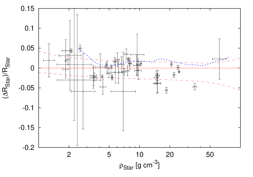
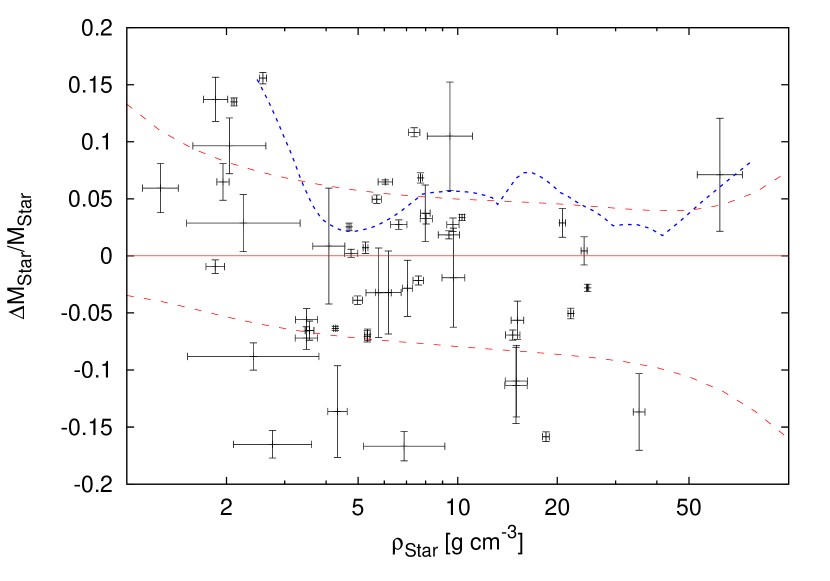
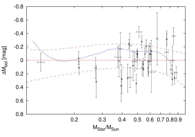
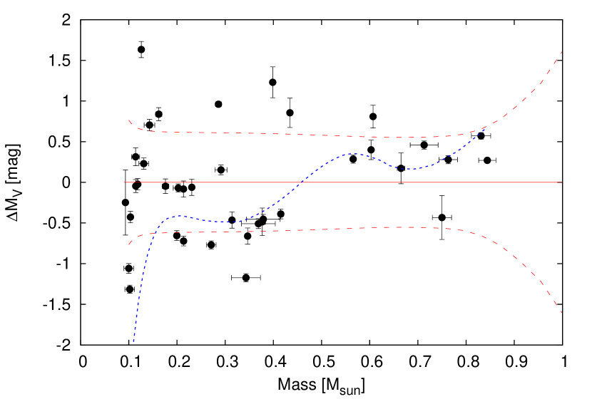
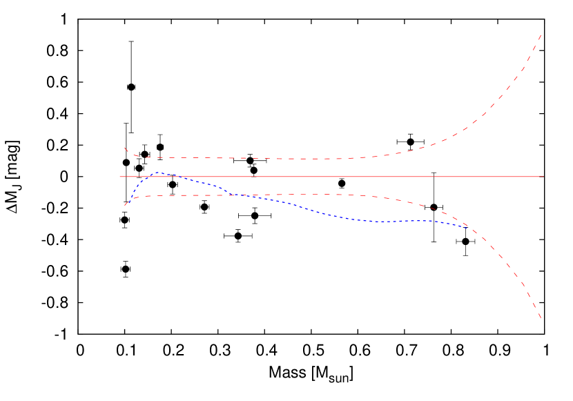
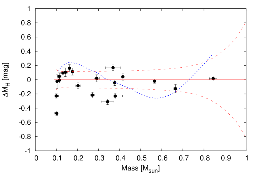
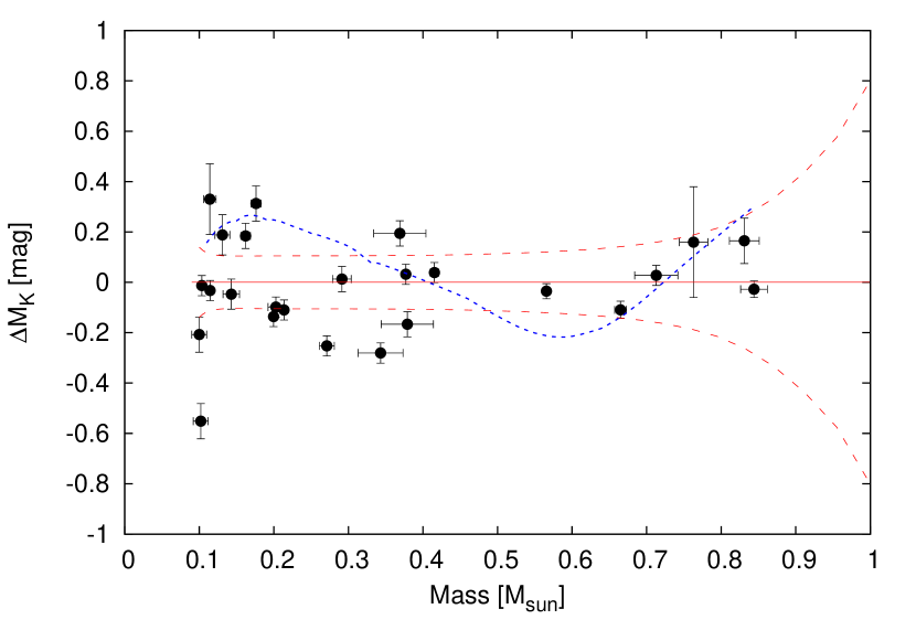
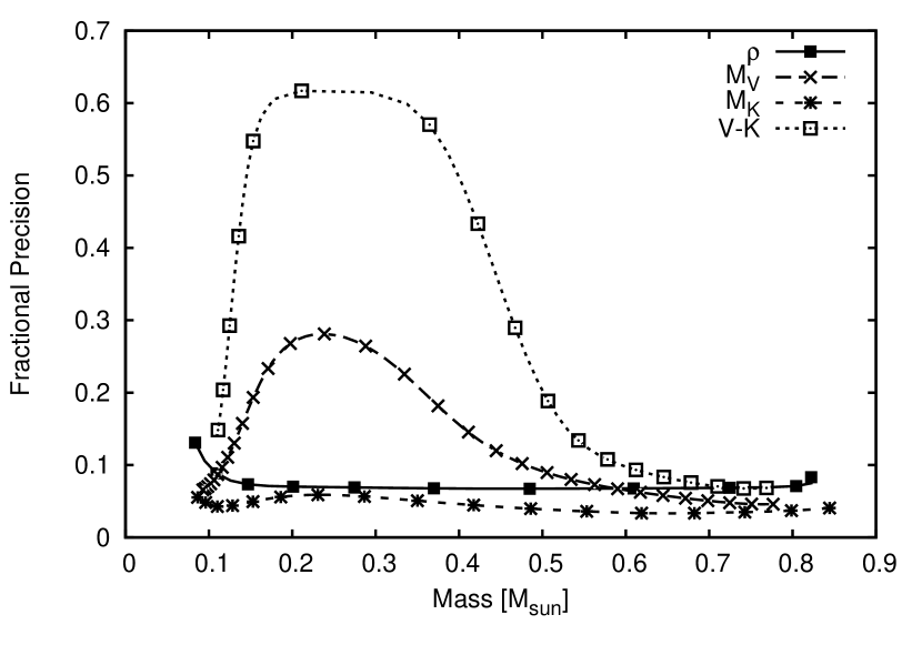
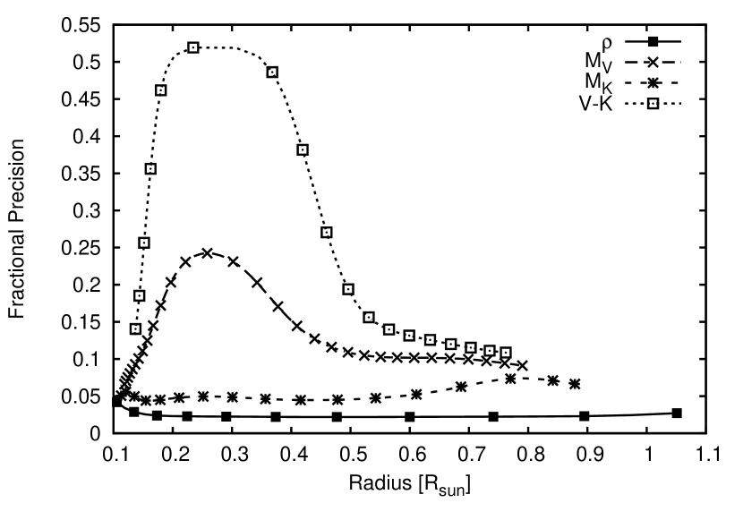
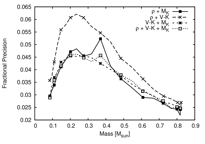
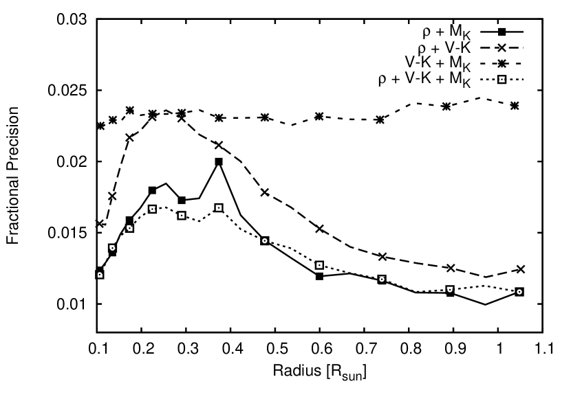
Figure 6 shows the fit between $l\rho$, $lM$ and $lR$, and between $lM$ and $M_{\rm bol}$, together with the residuals from this model, Figure 7 shows the relations between effective temperature and the $V$, $J$, $H$, and $K$ bolometric corrections, Figure 8 shows the relation between mass and the absolute magnitudes in each of these filters, and Figure 9 shows the residuals from the fits in Figure 8. Our model yields intrinsic scatters of $\sim 2$% in radius and $\sim 7$% in mass, and $4$% to $10$% in effective temperature (between $0.2$ mag and $0.5$ mag in bolometric magnitudes) given a value for $\rho_{\star}$. Figure 10 compares the precision in the inferred mass and radius implied by this modeling when using a single parameter to constrain the stellar properties (either $\rho_{\star}$, $M_{V}$, $M_{K}$ or $V-K$), and when using various combinations of observables. Assuming no observational uncertainties, $M_{K}$ is the highest precision stellar mass indicator, while $\rho_{\star}$ is the highest precision stellar radius indicator. By combining $\rho_{\star}$ with a photometric indicator, such as $M_{K}$, it is possible to improve the precision in mass and radius by up to a factor of two compared to the precision allowed by using only $\rho_{\star}$.

Note that due to the somewhat higher scatter in the stellar parameters at the high mass end, and the small number of stars constraining the fit at this end, we find that the stellar mass as a function of density reaches a local maximum of $\sim 0.8$ $M_{\sun}$ at $\rho\sim 1.5$ $\rm g\,cm^{-3}$. We therefore do not suggest using these models for stars with $M>0.8$ $M_{\sun}$, or spectral types earlier than K5.

It is worth comparing our modeling to that done by Johnson et al. (2011) and Johnson et al. (2012). One significant difference is the treatment of metallicity. Johnson et al. (2011) include a correlation between metallicity and $\Delta M_{K}$ (Johnson & Apps, 2009), while Johnson et al. (2012) include an additional correlation between metallicity and $\Delta J-K$ in their modelling. We choose not to include metallicity explicitly in our model due to the lack of a large sample of M dwarfs with well-measured masses, radii and metallicities. Lacking such a dataset, it is not possible to determine the effect of metallicity on all of the relations considered. Instead the metallicity is assumed to contribute to the intrinsic uncertainty in the $\rho\rightarrow R$ and $M\rightarrow M_{\rm bol}$ relations, measured using the $S_{R}$ and $S_{Mbol}$ parameters. While, like us, Johnson et al. (2011) use eclipsing binaries in calibrating the mass–radius relation, their sample is the Ribas (2006) catalog which contained only 14 stars with $M<0.8$ $M_{\sun}$, of which only 10 had masses and radii measured to better than 5% precision. Johnson et al. (2012), on the other hand, choose to use stars with interferometrically measured radii from Boyajian et al. (2012) due to the possibility that the eclipsing binaries are systematically inflated compared to single stars. While these stars have directly measured radii, their masses must be estimated using an assumed mass–luminosity relation. The few long period, low-mass eclipsing binaries which have been studied have parameters that are consistent with the shorter period binaries (Irwin et al., 2011; Doyle et al., 2011), moreover Boyajian et al. (2012) find no systematic difference between the mass–radius relation determined from their single stars (for an assumed mass–luminosity relation), and the mass–radius relation determined from short period eclipsing binaries, so we choose to use the eclipsing binaries for which both masses and radii are measured directly.

Having established our empirical stellar model, we use it to determine the properties of HATS-6 by incorporating it directly into our light curve and RV curve fit. To do this we add the following terms to our likelihood function:

$$-\frac{1}{2}\sum_{\lambda}\left(\frac{M_{\lambda}(l\rho,dlR,dM_{\rm bol})+\Delta d+A_{\lambda}-m_{\lambda}}{\sigma_{\lambda}}\right)^{2}$$

$$-\frac{1}{2}\left(\left(\frac{dlR}{S_{R}}\right)^{2}+\left(\frac{dM_{\rm bol}}{S_{M}}\right)^{2}\right)$$ (9)

Where $M_{\lambda}$ is the predicted absolute magnitude in filter $\lambda$ given $dlR$, $dM_{\rm bol}$, and $l\rho$, which is determined from the other free parameters in the model ($b^{2}$, $\zeta/R_{\star}$, $P$, $\sqrt{e}\sin\omega$, $\sqrt{e}\cos\omega$, and $K$); $\Delta d$ is the distance modulus and $A_{\lambda}$ is the extinction; $m_{\lambda}$ is the observed magnitude; and $\sigma_{\lambda}$ is the magnitude uncertainty. The sum is over the filters $\lambda=V$, $J$, $H$, and $K$. The new parameters introduced in the fit are thus $dlR$, $dM_{\rm bol}$, $\Delta d$ and $A_{V}$. We restrict $A_{V}$ to be in the range $[0,0.175]$ where the upper limit is the total line-of-sight extinction from the Schlafly & Finkbeiner (2011) reddenning maps, and we assume the Cardelli et al. (1989) extinction law to relate $A_{V}$ to the extinction in the other band-passes. Given $l\rho$, $dlR$, and $dM_{\rm bol}$ at each link in the resulting Markov Chain, we then calculate all relevant stellar parameters, and dependent planetary parameters.

Using the empirical model we find $M_{\star}=0.574_{-0.027}^{+0.020}$ $M_{\sun}$ and $R_{\star}=0.570\pm 0.011$ $R_{\sun}$, assuming a circular orbit, and $M_{\star}=0.573\pm 0.031$ $M_{\sun}$ and $R_{\star}=0.567\pm 0.037$ $R_{\sun}$, allowing for an eccentric orbit. The mass and radius inferred assuming a circular orbit are slightly lower than, though consistent with, the parameters inferred using the Dartmouth isochrones ($M_{\star}=0.595\pm 0.017$ $M_{\sun}$, and $R_{\star}=0.5759\pm 0.0092$ $R_{\sun}$). The precision allowed by both the Dartmouth and empirical models are similar. When we allow the eccentricity to vary with our empirical model the constraint from the observed $V-K$ color of the star pulls the model to a lower eccentricity solution, yielding parameters that are consistent with those from the fixed-circular model. For the final parameters we suggest adopting those from the empirical stellar model, assuming a circular orbit. The adopted stellar parameters are listed in Table 9 while the planetary parameters are listed in Table 10.

Table 8 Transiting-planet hosting stars with similar properties to HATS-6.

Star	Mass	Radius	$V-K$	$\rho_{\star}$	Planet Mass	Planet Period	Reference
	$M_{\sun}$	$R_{\sun}$	mag	$\rm g\,cm^{-3}$	$M_{\rm J}$	day
GJ 3470	$0.541\pm 0.067$	$0.503\pm 0.063$	$4.281\pm 0.030$	$6.0\pm 2.4$	$0.0441\pm 0.0053$	$3.34$	1
WASP-80	$0.596\pm 0.035$	$0.593\pm 0.012$	$3.53\pm 0.23$	$4.040\pm 0.012$	$0.562\pm 0.027$	$3.07$	2,8
KIC 10905746	$0.578\pm 0.032$	$0.548\pm 0.026$	$3.94\pm 0.24$	$4.97\pm 0.54$	$\ldots$	$9.88$	3
WASP-43	$0.580\pm 0.050$	$0.598^{+0.034}_{-0.042}$	$3.212\pm 0.027$	$3.81^{+0.86}_{-0.51}$	$1.78\pm 0.10$	$0.81$	4
Kepler-45	$0.570\pm 0.059$	$0.539\pm 0.039$	$3.990\pm 0.058$	$5.12\pm 0.73$	$0.500\pm 0.061$	$2.46$	5,9
HAT-P-54	$0.645\pm 0.020$	$0.617\pm 0.013$	$3.179\pm 0.063$	$3.88\pm 0.27$	$0.760\pm 0.032$	$3.80$	6
Kepler-26	$0.650\pm 0.030$	$0.590\pm 0.030$	$3.352\pm 0.026$	$4.47\pm 0.71$	$\ldots$	$12.28$	7

References. — 1: Bonfils et al. (2012); 2: Triaud et al. (2013b); 3: Fischer et al. (2012); 4: Hellier et al. (2011); 5: Johnson et al. (2012); 6: Bakos et al. (2014); 7: Steffen et al. (2012); 8: Mancini et al. (2014); 9: Southworth (2012)

Table 9 Stellar parameters for HATS-6

Parameter	Value Isochrones	Value Empirical	Value Empirical
	Circ.	Circ.	Eccen.
Identifying Information
R.A. (h:m:s; 2MASS)	$05^{\mathrm{h}}52^{\mathrm{m}}35.22{\mathrm{s}}$	$\ldots$	$\ldots$
Dec. (d:m:s; 2MASS)	$-19{\arcdeg}01{\arcmin}54.0{\arcsec}$	$\ldots$	$\ldots$
2MASS ID	2MASS 05523523-1901539	$\ldots$	$\ldots$
Spectroscopic properties
$T_{\rm eff\star}$ (K)	$3770\pm 100$	$\ldots$	$\ldots$
$\rm[Fe/H]$	$0.200\pm 0.091$	$\ldots$	$\ldots$
Photometric properties
$B$ (mag; APASS)	$16.664\pm 0.043$	…	…
$V$ (mag; APASS)	$15.160\pm 0.024$	…	…
$J$ (mag; 2MASS)	$12.046\pm 0.024$	…	…
$H$ (mag; 2MASS)	$11.397\pm 0.023$	…	…
$K_{s}$ (mag; 2MASS)	$11.224\pm 0.023$	…	…
Derived properties
$M_{\star}$ ($M_{\sun}$)	$0.595\pm 0.017$	$0.574_{-0.027}^{+0.020}$	$0.573\pm 0.031$
$R_{\star}$ ($R_{\sun}$)	$0.5759\pm 0.0092$	$0.570\pm 0.011$	$0.567\pm 0.037$
$T_{\rm eff\star}$ (K)	$3872\pm 53$	$3724\pm 18$	$3722\pm 19$
$\rho_{\star}$ (cgs)	$4.40\pm 0.13$	$4.36\pm 0.15$	$4.42_{-0.47}^{+0.75}$
$\log{g_{\star}}$ (cgs)	$4.6920\pm 0.0077$	$4.683\pm 0.010$	$4.689\pm 0.038$
$L_{\star}$ ($L_{\sun}$)	$0.0670\pm 0.0054$	$0.0558\pm 0.0024$	$0.0555\pm 0.0073$
$M_{V}$ (mag)	$9.43\pm 0.19$	$9.209\pm 0.075$	$9.22\pm 0.15$
$M_{K}$ (mag,ESO)	$5.079\pm 0.065$	$5.387\pm 0.043$	$5.40\pm 0.14$
Age (Gyr)	$8.1\pm 4.3$	$\ldots$	$\ldots$
Distance (pc)	$172.6\pm 5.5$	$148.4\pm 3.3$	$147.8_{-9.4}^{+7.0}$

Table 10Orbital and planetary parameters

Parameter	Value Isochrones	Value Empirical	Value Empirical
	Circ.	Circ.	Eccen.
Light curve parameters
$P$ (days)	$3.3252721\pm 0.0000020$	$3.3252725\pm 0.0000021$	$3.3252726\pm 0.0000021$
$T_{c}$ (${\rm BJD}$)	$2456643.740560\pm 0.000089$	$2456643.740580\pm 0.000084$	$2456643.740600\pm 0.000094$
$T_{14}$ (days)	$0.08497\pm 0.00036$	$0.08504\pm 0.00045$	$0.08508\pm 0.00037$
$T_{12}=T_{34}$ (days)	$0.01542\pm 0.00035$	$0.01545\pm 0.00039$	$0.01549\pm 0.00034$
$a/R_{\star}$	$13.70\pm 0.13$	$13.65\pm 0.15$	$13.71_{-0.50}^{+0.73}$
$\zeta/R_{\star}$	$28.608\pm 0.066$	$28.612\pm 0.077$	$28.605\pm 0.066$
$R_{p}/R_{\star}$	$0.17974\pm 0.00069$	$0.17978\pm 0.00077$	$0.17986\pm 0.00070$
$b\equiv a\cos i/R_{\star}$	$0.428_{-0.022}^{+0.016}$	$0.427_{-0.021}^{+0.020}$	$0.429_{-0.020}^{+0.017}$
$i$ (deg)	$88.210\pm 0.093$	$88.210\pm 0.084$	$88.23\pm 0.16$
Limb-darkening coefficients
$a_{g}$ (linear term)	$0.4748$	$\cdots$	$\cdots$
$b_{g}$ (quadratic term)	$0.3277$	$\cdots$	$\cdots$
$a_{r}$ (linear term)	$0.4403$	$\cdots$	$\cdots$
$b_{r}$ (quadratic term)	$0.3333$	$\cdots$	$\cdots$
$a_{i}$	$0.4092$	$\cdots$	$\cdots$
$b_{i}$	$0.2831$	$\cdots$	$\cdots$
$a_{z}$	$0.2843$	$\cdots$	$\cdots$
$b_{z}$	$0.3315$	$\cdots$	$\cdots$
$a_{R}$	$0.4091$	$\cdots$	$\cdots$
$b_{R}$	$0.3382$	$\cdots$	$\cdots$
RV parameters
$K$ ($\rm m\,s^{-1}$)	$68\pm 15$	$63\pm 14$	$64\pm 15$
$\sqrt{e}\cos\omega$	$\ldots$	$\ldots$	$0.09\pm 0.19$
$\sqrt{e}\sin\omega$	$\ldots$	$\ldots$	$-0.03\pm 0.16$
$e\cos\omega$	$\ldots$	$\ldots$	$0.015_{-0.028}^{+0.085}$
$e\sin\omega$	$\ldots$	$\ldots$	$-0.004_{-0.058}^{+0.031}$
$e$	$0$, fixed	$0$, fixed	$0.053\pm 0.060$
$\omega$	$\ldots$	$\ldots$	$230\pm 120$
PFS RV jitter ($\rm m\,s^{-1}$)	$26\pm 14$	$26\pm 11$	$26.2\pm 9.9$
FEROS RV jitter ($\rm m\,s^{-1}$)	$51\pm 56$	$41\pm 45$	$39\pm 41$
HARPS RV jitter ($\rm m\,s^{-1}$)	$0\pm 15$	$0\pm 20$	$0\pm 50$
Planetary parameters
$M_{p}$ ($M_{\rm J}$)	$0.357_{-0.089}^{+0.059}$	$0.319\pm 0.070$	$0.321\pm 0.076$
$R_{p}$ ($R_{\rm J}$)	$1.008\pm 0.019$	$0.998\pm 0.019$	$0.994\pm 0.065$
$C(M_{p},R_{p})$	$-0.00$	$0.08$	$0.16$
$\rho_{p}$ ($\rm g\,cm^{-3}$)	$0.431_{-0.111}^{+0.076}$	$0.399\pm 0.089$	$0.406_{-0.098}^{+0.133}$
$\log g_{p}$ (cgs)	$2.940_{-0.130}^{+0.064}$	$2.90\pm 0.12$	$2.91\pm 0.12$
$a$ (AU)	$0.03667\pm 0.00035$	$0.03623_{-0.00057}^{+0.00042}$	$0.03621\pm 0.00065$
$T_{\rm eq}$ (K)	$740\pm 12$	$712.8\pm 5.1$	$711\pm 18$
$\Theta$	$0.0436_{-0.0112}^{+0.0069}$	$0.0404\pm 0.0089$	$0.0409\pm 0.0100$
$\langle F\rangle$ ($10^{7}$$\rm erg\,s^{-1}\,cm^{-2}$)	$6.80\pm 0.44$	$5.84\pm 0.17$	$5.78\pm 0.60$

4. Discussion

In this paper we have presented the discovery of the HATS-6 transiting planet system by the HATSouth survey. We found that HATS-6b has a mass of $0.319\pm 0.070{}$ $M_{\rm J}$, radius of $0.998\pm 0.019{}$ $R_{\rm J}$ and orbits a star with a mass of $0.574_{-0.027}^{+0.020}{}$ $M_{\sun}$. HATS-6 is one of only four stars with $M\lesssim 0.6$ $M_{\sun}$ known to host a short period gas giant planet (the other three are WASP-80, WASP-43, and Kepler-45; see Table 3.3.2). This is illustrated in Figure 11 where we plot planet mass against the host star mass. We note that the published masses for these stars come from a disparate set of methods. Applying the empirical relations developed in this paper (Section 3.3.2) to these two systems, using $\rho_{\star}$, $V$, $J$, $H$ and $K_{S}$ as observables, we find masses of $0.614\pm 0.031$ $M_{\sun}$, and $0.601\pm 0.031$ $M_{\sun}$, for WASP-43 and WASP-80, respectively, slightly higher than the published values of $0.580\pm 0.050$ $M_{\sun}$ and $0.596\pm 0.035$ $M_{\sun}$. This same method yields a mass of $0.534\pm 0.034$ $M_{\sun}$ for Kepler-45, which is a bit lower than the published value of $0.570\pm 0.059$ $M_{\sun}$.

HATS-6b also has some of the deepest transits known, with $(R_{p}/R_{\star})^{2}=0.0323\pm 0.0003$. There are only two known planets with deeper transits than HATS-6b: Kepler-45b ($(R_{p}/R_{\star})^{2}=0.0362\pm 0.0054$; Southworth, 2012), and WTS-2b, a hot Jupiter on a very short period orbit around a K2 dwarf star ($(R_{p}/R_{\star})^{2}=0.0347\pm 0.0008$; Birkby et al., 2014). One other system with transit depths close to that of HATS-6 is WASP-80b ($(R_{p}/R_{\star})^{2}=0.0292\pm 0.0001$; Mancini et al., 2014). Figure 11 illustrates this as well, plotting the transit depth vs. planet mass.

With an early M dwarf host star, HATS-6b receives substantially less stellar irradiation than planets with the same orbital period around Sun-like stars. As a result the equilibrium temperature, assuming zero albedo, is a relatively mild $712.8\pm 5.1{}$ K. The atmospheric chemistry at this temperature is expected to be notably different from other hotter planets, with a greater abundance of CH₄ and associated hydro-carbon hazes (Howe & Burrows, 2012; Fortney et al., 2013). This makes HATS-6b a potentially interesting target for studying the atmospheric properties of a warm gas giant. In the bottom two panels of Figure 11 we plot the approximate $K$-band transmission spectrum S/N, and $4.5$ $\mu$m occultation spectrum S/N vs. T_eq. In both cases we normalize the S/N to that of the prototypical hot Jupiter HD 189733b. For the transmission spectrum S/N we use the relation (e.g., Winn, 2010):

$${\rm S/N}\propto\frac{2R_{P}HN_{H}}{R_{\star}^{2}}\sqrt{T_{14}F_{K}}$$ (10)

where $H=k_{B}T_{\rm eq}/\mu g_{P}$, $\mu$ is the mean molecular weight (we assume $3.347\times 10^{-27}$ kg for a pure H₂ atmosphere), $g_{P}$ is the surface gravity of the planet, $T_{14}$ is the transit duration, $F_{K}$ is the $K$-band flux of the star in Janskys, and $N_{H}$ is a constant of order unity (we assume 1) depending on the particular spectroscopic feature under consideration. The term $\sqrt{T_{14}F_{K}}$ is included because the photometric noise is proportional to $1/\sqrt{F_{K}}$ and the number of in transit measurements that can be made is proportional to $T_{14}$ (meaning the noise goes as $1/\sqrt{T_{14}}$). We neglect the constant of proportionality on the right-hand-side of eq. 10 needed to make the expression for S/N unitless. For the occultation spectrum S/N we use the relation (e.g., Winn, 2010):

$${\rm S/N}\propto\left(\frac{R_{P}}{R_{\star}}\right)^{2}\frac{\exp(hc/k_{B}\lambda T_{\rm eff})-1}{\exp(hc/k_{B}\lambda T_{\rm eq})-1}\sqrt{T_{14}F_{4.5}}$$ (11)

where $h$ is Planck’s constant, $c$ is the speed of light, $k_{B}$ is Boltmann’s constant, $T_{\rm eff}$ is the stellar effective temperature, $\lambda$ is the effective wavelength (we assume 4.5 $\mu$m), and $F_{4.5}$ is the 4.5 $\mu$m flux of the star in Janskys.

We find that HATS-6b has the highest expected S/N transmission spectrum among known gas giant planets with $T_{\rm eq}<750$ K. Regarding occultations, HATS-6b has the second highest expected S/N at 4.5 $\mu$m among gas giant planets with $T_{\rm eq}<750$ K after HD 80606b (Laughlin et al., 2009, the expected S/N for HATS-6b is $\sim 50$% that of HD 80606b).

Perhaps the most relevant planet for comparison is WASP-80b, a hot Jupiter with $T_{\rm eq}=825\pm 20$ K (Mancini et al., 2014), with a similar transit depth to HATS-6b, but orbiting a somewhat brighter star. High-precision ground-based photometric transit observations of this system over several optical and near infrared band-passes have been presented by Mancini et al. (2014) and Fukui et al. (2014), which have provided suggestive evidence for the existence of a haze in the atmosphere. The expected transmission S/N for HATS-6b is approximately $0.4$ times that of WASP-80b, so measuring the transmission spectrum for HATS-6b will be challenging, but not out of reach for ground-based facilities. HATS-6b is also a promising target for the NASA James Webb Space Telescope mission, currently scheduled for launch in 2018.

We checked whether the simultaneous optical multi-filter GROND observations that we have already obtained for HATS-6 can be used to probe the transmission spectrum. We fit a Mandel & Agol (2002) transit model to each of the GROND $g$, $r$, $i$ and $z$ light curves, fixing all transit parameters to the best-fit values for the system, except for $R_{p}/R_{\star}$, which we allow to vary independently for each band-pass. We find that values for $R_{p}/R_{\star}$ values are consistent with a flat transmission spectrum, to within the uncertainties. Additional observations would be needed to detect spectroscopic features in the atmosphere of HATS-6b.

In order to characterize the host star HATS-6 we have also presented a new set of empirical stellar models applicable to main-sequence stars with $M<0.80$ $M_{\sun}$. We use eclipsing binaries as well as resolved binaries with masses and measured absolute magnitudes to determine empirical relations between $\rho_{\star}$ and $R$ (and thus $\rho_{\star}$ and $M$), between $M$ and $M_{\rm bol}$, and between $T_{\rm eff}$ and the $V$, $J$, $H$ and $K$-band bolometric corrections. We perform a global fit to the available data, determining the intrinsic scatter in the relations in a self-consistent manner. We find that from the density alone it is possible to measure the mass of a $\sim 0.6$ $M_{\sun}$ star to $\sim 7$% precision, and the radius to $\sim 2$% precision. These precisions may be improved by up to a factor of two, to $\sim 3$% and $\sim 1$%, respectively, by incorporating additional photometric data. The relations presented here are similar to those presented by Johnson et al. (2011) and Johnson et al. (2012) except that we do not attempt to incorporate metallicity directly into the model (it contributes instead to the inherent scatter in the relations), and we use a much larger sample of eclipsing binaries than previously considered. Future improvements to our model may be made by incorporating metallicity information directly into the model, but this will require a large sample of stars with measured masses, radii, absolute magnitudes, and metallicities.

Finally, we note that the discovery of HATS-6b is a demonstration of the enhanced sensitivity of HATSouth to planets around low-mass K and M dwarf stars relative to other wide-field ground based surveys, such as HATNet or WASP. The reason for this enhanced sensitivity is the larger aperture optics used by HATSouth, providing higher photometric precision for fainter stars. HATSouth yields better than 2% precision, per 240 s integration, for stars down to $r\sim 14.5$. For comparison, if using the same integration time as HATSouth, HATNet would yield 2% precision for stars with $r\lesssim 13$. Based on the TRILEGAL Galactic models (Girardi et al., 2005) we estimate that there are $\sim 230000$ stars with $M<0.6$ $M_{\sun}$, $r<14.5$ in the Southern sky, and at least $10^{\circ}$ from the Galactic disk that could be observed by HATSouth. This is nearly a factor of ten more than the number of stars with $M<0.6$ $M_{\sun}$ and $r<13.0$ in the Northern sky that could be observed by HATNet to the same photometric precision. While in principle the discovery of HATS-6b may be used to infer the occurrence rate of hot Jupiters around early M dwarfs (e.g., Gaidos & Mann, 2014), in practice this requires a careful calibration of our transit detection efficiency over the sample of M dwarfs that we have observed. This is beyond the scope of the present paper, but will be the subject of future work.

Figure 11.— Comparison of the HATS-6 system to other known transiting exoplanet systems with $M_{P}>0.1$ $M_{\rm J}$. In each case HATS-6 is indicated by the filled red triangle, while other objects are indicated by filled black circles. Top Left: Planet mass vs. transit depth as measured by $(R_{p}/R_{\star})^{2}$. Top Right: Host star mass vs. planet mass. Bottom Left: Estimated S/N of a single occultation event at 4.5 $\mu$m normalized to that of HD 189733b. Bottom Right: Estimated S/N of a transmission spectrum signal from one transit, assuming a pure H₂ atmosphere, and observed at $K$-band, normalized to that of HD 189733b. HATS-6 has some of the deepest transits of known transiting planet systems, it is also one of the lowest mass stars known to host a transiting gas giant planet. In terms of atmospheric characterization it is one of the highest S/N targets with $T_{\rm eq}<750$ K for both occultation and transmission spectroscopy.

References

- Adams & Laughlin (2006) Adams, F. C., & Laughlin, G. 2006, ApJ, 649, 1004
- Bakos et al. (2010) Bakos, G. Á., Torres, G., Pál, A., et al. 2010, ApJ, 710, 1724
- Bakos et al. (2012) Bakos, G. Á., Hartman, J. D., Torres, G., et al. 2012, AJ, 144, 19
- Bakos et al. (2013) Bakos, G. Á., Csubry, Z., Penev, K., et al. 2013, PASP, 125, 154
- Bakos et al. (2014) Bakos, G. Á., Hartman, J. D., Bhatti, W., et al. 2014, ArXiv e-prints, 1404.4417
- Bayliss et al. (2013) Bayliss, D., Zhou, G., Penev, K., et al. 2013, AJ, 146, 113
- Bedford et al. (1987) Bedford, D. K., Fuensalida, J. J., & Arevalo, M. J. 1987, A&A, 182, 264
- Birkby et al. (2012) Birkby, J., Nefs, B., Hodgkin, S., et al. 2012, MNRAS, 426, 1507
- Birkby et al. (2014) Birkby, J. L., Cappetta, M., Cruz, P., et al. 2014, MNRAS, 440, 1470
- Bonfils et al. (2012) Bonfils, X., Gillon, M., Udry, S., et al. 2012, A&A, 546, A27
- Boyajian et al. (2012) Boyajian, T. S., von Braun, K., van Belle, G., et al. 2012, ApJ, 757, 112
- Brown et al. (2013) Brown, T. M., Baliber, N., Bianco, F. B., et al. 2013, PASP, 125, 1031
- Butler et al. (1996) Butler, R. P., Marcy, G. W., Williams, E., et al. 1996, PASP, 108, 500
- Cardelli et al. (1989) Cardelli, J. A., Clayton, G. C., & Mathis, J. S. 1989, ApJ, 345, 245
- Carter et al. (2011) Carter, J. A., Fabrycky, D. C., Ragozzine, D., et al. 2011, Science, 331, 562
- Claret (2004) Claret, A. 2004, A&A, 428, 1001
- Coelho et al. (2005) Coelho, P., Barbuy, B., Meléndez, J., Schiavon, R. P., & Castilho, B. V. 2005, A&A, 443, 735
- Crane et al. (2010) Crane, J. D., Shectman, S. A., Butler, R. P., et al. 2010, in Society of Photo-Optical Instrumentation Engineers (SPIE) Conference Series, Vol. 7735, Society of Photo-Optical Instrumentation Engineers (SPIE) Conference Series
- Deeg & Doyle (2001) Deeg, H. J., & Doyle, L. R. 2001, in Third Workshop on Photometry, ed. W. J. Borucki & L. E. Lasher, 85
- Delfosse et al. (2000) Delfosse, X., Forveille, T., Ségransan, D., et al. 2000, A&A, 364, 217
- Demory et al. (2009) Demory, B.-O., Ségransan, D., Forveille, T., et al. 2009, A&A, 505, 205
- Dimitrov & Kjurkchieva (2010) Dimitrov, D. P., & Kjurkchieva, D. P. 2010, MNRAS, 406, 2559
- Dopita et al. (2007) Dopita, M., Hart, J., McGregor, P., et al. 2007, Ap&SS, 310, 255
- Dotter et al. (2008) Dotter, A., Chaboyer, B., Jevremović, D., et al. 2008, ApJS, 178, 89
- Doyle et al. (2011) Doyle, L. R., Carter, J. A., Fabrycky, D. C., et al. 2011, Science, 333, 1602
- Eastman et al. (2013) Eastman, J., Gaudi, B. S., & Agol, E. 2013, PASP, 125, 83
- Edelson & Krolik (1988) Edelson, R. A., & Krolik, J. H. 1988, ApJ, 333, 646
- Enoch et al. (2010) Enoch, B., Collier Cameron, A., Parley, N. R., & Hebb, L. 2010, A&A, 516, A33
- Feiden et al. (2011) Feiden, G. A., Chaboyer, B., & Dotter, A. 2011, ApJ, 740, L25
- Fernandez et al. (2009) Fernandez, J. M., Latham, D. W., Torres, G., et al. 2009, ApJ, 701, 764
- Fischer et al. (2012) Fischer, D. A., Schwamb, M. E., Schawinski, K., et al. 2012, MNRAS, 419, 2900
- Fortney et al. (2013) Fortney, J. J., Mordasini, C., Nettelmann, N., et al. 2013, ApJ, 775, 80
- Fukui et al. (2014) Fukui, A., Kawashima, Y., Ikoma, M., et al. 2014, ArXiv e-prints, 1406.3261
- Gaidos & Mann (2014) Gaidos, E., & Mann, A. W. 2014, ArXiv e-prints, 1406.4071
- Girardi et al. (2005) Girardi, L., Groenewegen, M. A. T., Hatziminaoglou, E., & da Costa, L. 2005, A&A, 436, 895
- Greiner et al. (2008) Greiner, J., Bornemann, W., Clemens, C., et al. 2008, PASP, 120, 405
- Grundahl et al. (2008) Grundahl, F., Clausen, J. V., Hardis, S., & Frandsen, S. 2008, A&A, 492, 171
- Hansen & Barman (2007) Hansen, B. M. S., & Barman, T. 2007, ApJ, 671, 861
- Hartman et al. (2011) Hartman, J. D., Bakos, G. Á., Noyes, R. W., et al. 2011, AJ, 141, 166
- Hartman et al. (2012) Hartman, J. D., Bakos, G. Á., Béky, B., et al. 2012, AJ, 144, 139
- Haywood (2001) Haywood, M. 2001, MNRAS, 325, 1365
- Hellier et al. (2011) Hellier, C., Anderson, D. R., Collier Cameron, A., et al. 2011, A&A, 535, L7
- Hełminiak et al. (2012) Hełminiak, K. G., Konacki, M., RóŻyczka, M., et al. 2012, MNRAS, 425, 1245
- Howard et al. (2012) Howard, A. W., Marcy, G. W., Bryson, S. T., et al. 2012, ApJS, 201, 15
- Howe & Burrows (2012) Howe, A. R., & Burrows, A. S. 2012, ApJ, 756, 176
- Irwin et al. (2009) Irwin, J., Charbonneau, D., Berta, Z. K., et al. 2009, ApJ, 701, 1436
- Irwin et al. (2011) Irwin, J. M., Quinn, S. N., Berta, Z. K., et al. 2011, ApJ, 742, 123
- Johnson et al. (2010) Johnson, J. A., Aller, K. M., Howard, A. W., & Crepp, J. R. 2010, PASP, 122, 905
- Johnson & Apps (2009) Johnson, J. A., & Apps, K. 2009, ApJ, 699, 933
- Johnson et al. (2011) Johnson, J. A., Apps, K., Gazak, J. Z., et al. 2011, ApJ, 730, 79
- Johnson et al. (2012) Johnson, J. A., Gazak, J. Z., Apps, K., et al. 2012, AJ, 143, 111
- Jordán et al. (2014) Jordán, A., Brahm, R., Bakos, G. Á., et al. 2014, AJ, 148, 29
- Kaufer & Pasquini (1998) Kaufer, A., & Pasquini, L. 1998, in Society of Photo-Optical Instrumentation Engineers (SPIE) Conference Series, Vol. 3355, Optical Astronomical Instrumentation, ed. S. D’Odorico, 844–854
- Kovács et al. (2005) Kovács, G., Bakos, G., & Noyes, R. W. 2005, MNRAS, 356, 557
- Kovács et al. (2002) Kovács, G., Zucker, S., & Mazeh, T. 2002, A&A, 391, 369
- Kraus et al. (2011) Kraus, A. L., Tucker, R. A., Thompson, M. I., Craine, E. R., & Hillenbrand, L. A. 2011, ApJ, 728, 48
- Kurtz (1985) Kurtz, D. W. 1985, MNRAS, 213, 773
- Laughlin et al. (2009) Laughlin, G., Deming, D., Langton, J., et al. 2009, Nature, 457, 562
- Lopez-Morales et al. (2006) Lopez-Morales, M., Orosz, J. A., Shaw, J. S., et al. 2006, ArXiv Astrophysics e-prints
- López-Morales & Ribas (2005) López-Morales, M., & Ribas, I. 2005, ApJ, 631, 1120
- Mancini et al. (2014) Mancini, L., Southworth, J., Ciceri, S., et al. 2014, A&A, 562, A126
- Mandel & Agol (2002) Mandel, K., & Agol, E. 2002, ApJ, 580, L171
- Mayor et al. (2003) Mayor, M., Pepe, F., Queloz, D., et al. 2003, The Messenger, 114, 20
- Mohler-Fischer et al. (2013) Mohler-Fischer, M., Mancini, L., Hartman, J. D., et al. 2013, A&A, 558, A55
- Morales et al. (2009) Morales, J. C., Ribas, I., Jordi, C., et al. 2009, ApJ, 691, 1400
- Nefs et al. (2013) Nefs, S. V., Birkby, J. L., Snellen, I. A. G., et al. 2013, MNRAS, 431, 3240
- Neves et al. (2014) Neves, V., Bonfils, X., Santos, N. C., et al. 2014, ArXiv e-prints, 1406.6127
- Ofir et al. (2012) Ofir, A., Gandolfi, D., Buchhave, L., et al. 2012, MNRAS, 423, L1
- Pál (2012) Pál, A. 2012, MNRAS, 421, 1825
- Penev et al. (2013) Penev, K., Bakos, G. Á., Bayliss, D., et al. 2013, AJ, 145, 5
- Popper (1994) Popper, D. M. 1994, AJ, 108, 1091
- Popper (1997) —. 1997, AJ, 114, 1195
- Rajpurohit et al. (2013) Rajpurohit, A. S., Reylé, C., Allard, F., et al. 2013, A&A, 556, A15
- Ribas (2003) Ribas, I. 2003, A&A, 398, 239
- Ribas (2006) —. 2006, Ap&SS, 304, 89
- Sandquist et al. (2013) Sandquist, E. L., Mathieu, R. D., Brogaard, K., et al. 2013, ApJ, 762, 58
- Schlafly & Finkbeiner (2011) Schlafly, E. F., & Finkbeiner, D. P. 2011, ApJ, 737, 103
- Ségransan et al. (2003) Ségransan, D., Kervella, P., Forveille, T., & Queloz, D. 2003, A&A, 397, L5
- Southworth (2011) Southworth, J. 2011, MNRAS, 417, 2166
- Southworth (2012) —. 2012, MNRAS, 426, 1291
- Steffen et al. (2012) Steffen, J. H., Fabrycky, D. C., Ford, E. B., et al. 2012, MNRAS, 421, 2342
- ter Braak (2006) ter Braak, C. J. F. 2006, Statistics and Computing, 16, 239
- Torres (2013) Torres, G. 2013, Astronomische Nachrichten, 334, 4
- Torres et al. (2010) Torres, G., Andersen, J., & Giménez, A. 2010, A&A Rev., 18, 67
- Torres et al. (2002) Torres, G., Boden, A. F., Latham, D. W., Pan, M., & Stefanik, R. P. 2002, AJ, 124, 1716
- Torres & Ribas (2002) Torres, G., & Ribas, I. 2002, ApJ, 567, 1140
- Torres et al. (2007) Torres, G., Bakos, G. Á., Kovács, G., et al. 2007, ApJ, 666, L121
- Triaud et al. (2013a) Triaud, A. H. M. J., Hebb, L., Anderson, D. R., et al. 2013a, A&A, 549, A18
- Triaud et al. (2013b) Triaud, A. H. M. J., Anderson, D. R., Collier Cameron, A., et al. 2013b, A&A, 551, A80
- Valenti & Fischer (2005) Valenti, J. A., & Fischer, D. A. 2005, ApJS, 159, 141
- Winn (2010) Winn, J. N. 2010, ArXiv e-prints, 1001.2010
- Zhou et al. (2014) Zhou, G., Bayliss, D., Hartman, J. D., et al. 2014, MNRAS, 437, 2831