Modeling Basic Aspects of Cyber-Physical Systems, Part II

Abstract

We continue to consider the question of what language features are needed to effectively model cyber-physical systems (CPS). In previous work, we proposed using a core language as a way to study this question, and showed how several basic aspects of CPS can be modeled clearly in a language with a small set of constructs. This paper reports on the result of our analysis of two, more complex, case studies from the domain of rigid body dynamics. The first one, a quadcopter, illustrates that previously proposed core language can support larger, more interesting systems than previously shown. The second one, a serial robot, provides a concrete example of why we should add language support for static partial derivatives, namely that it would significantly improve the way models of rigid body dynamics can be expressed.

I Introduction

The increasing computational power embedded in everyday products promises to revolutionize the way we live. At the same time, the tight coupling between computational and physical mechanisms, often described as cyber-physical systems (CPSs), poses a challenge for the traditional product development cycles, particularly in physical testing. For example, car manufacturers are concerned about the amount of physical testing necessary to assure the safety of autonomous vehicles. Physical testing has been used to assess the qualities of new products for many years. One of its key ingredients is devising a collection of specific test scenarios. But the presence of even simple computational components can make it difficult to identify enough test scenarios to exercise more than a minute fraction of the possible behaviors of the system. In addition, physical testing is very expensive because it only detects flaws at the end of the product development process after physical prototypes have been constructed. These realities are spurring the CPS developers to rethink traditional methods and processes for developing and testing new products.

Computer simulations [2] performing virtual experiments [3] can be used to reduce the cost of physical tests. Virtual testing can be used to quickly eliminate obviously bad designs. It can also help build confidence that a new design can pass test scenarios developed by an independent party [4]. However, creating a framework for conducting virtual experiments requires a concerted, interdisciplinary effort to address a wide range of challenges, including: 1) educating designers in the cyber-physical aspects of the products they will develop, both in terms of how these aspects are modeled, and what types of system-level behaviors are generated; and 2) developing expressive, efficient, and robust modeling and simulation tools to support the innovation process. At each stage in the design process, the underlying models should be easy to understand and analyze. Moreover, it should be easy to deduce the mathematical relationship between the models used in successive stages.

Both challenges can be addressed by better language-based technologies for modeling and simulation. An effective model should have clear and unambiguous semantics that can readily be simulated, showing how the model behaves in concrete scenarios. Engineering methods centered around a notion of executable or effective models can have profound positive impacts on the pace of advancement of knowledge and engineering practice.

I-A The Accessibility Challenge

Designing a future smart vehicle or home requires expertise from a number of different disciplines. Even when we can assemble the necessary team of experts, they often lack a common language for discussing key issues – treated differently across disciplines – that arise in CPS design.

A critical step towards addressing this accessibility challenge is to discover (and not “invent”) a lingua franca (or “common language”) that can break down artificial linguistic barriers between various scientific and engineering disciplines. Part of such a common language will be a natural language that includes a collection of technical terms from the domain of CPS, and that enables experts to efficiently express common model constructions; part will be executable (meaning computationally effective) modeling formalisms made up from a subset of the mathematical notation already in use. Language research can be particularly helpful in discovering the latter part [5]. Examples of such tools exist, but are usually not available as widely-used, multi-purpose tools. This is the case for languages such as Fortress [6] and equational languages [7, 8], as well as specialized, physics-specific or even multi-physics tools. When they are available as widely-used, multi-purpose tools, they generally cannot be viewed as executable formalisms. This is the case for most symbolic algebra tools.

I-B The Tool Chain Coherence Challenge

Based on our experience in several domains, it appears that scientists and engineers engaged in CPS design are often forced to transfer models through a chain of disparate, specialized design tools. Each tool has a clear purpose. For example, drafting tools like AutoCAD and Solidworks support creating images of new products; MATLAB, R, and Biopython support the simple programming of dynamics and control; and finally, tools like Simulink support the simulation of device operation  [5]. Between successive tools in this chain, there is often little or no formal communication. It is the responsibility of the CPS designer to translate any data or valuable knowledge to the next tool.

We believe that tool chain coherence should be approached from a linguistic point of view. Precise reasoning about models during each step of the design process can readily be supported by applying classical (programming) language design principles, including defining a formal semantics. Reasoning across design steps can be facilitated by applying two specific ideas from language design: 1) increasing the expressivity of a language to encompass multiple steps in the design process; and 2) automatically compiling models from one step to the next. The latter idea reduces manual work and eliminates opportunities for mistakes in the translation.

I-C Recapitulation of Part I

Part I of this work [1] identifies a set of prominent aspects that are common to CPS design, and shows the extent to which a small core language, which we call Acumen, supports the expression of these aspects. The earlier paper considers the following aspects:

1. Geometry and visual form

2. Mechanics and dynamics

3. Object composition

4. Control

5. Disturbances

6. Rigid body dynamics

and presents a series of examples illustrating the expressivity and convenience of the language for each of these aspects. In this narrative, the last aspect stands out as more open-ended and potentially challenging. The early paper considers a single case study involving a rigid body: a single link rod (two masses connected by a fixed-length bar). Thus, it does not address the issue of how well such a small language is suited to modeling larger rigid body systems.

I-D Contributions

Modeling continuous dynamics is only one aspect of CPS designs that we may need to model, but it is important because it is particularly difficult. This paper extends previous work by considering the linguistic demands posed by two larger case studies drawn from the rigid body domain. After a brief review of Acumen (Section II), the first case study we consider is a quadcopter, which is a complex, rigid body system that is often used as a CPS example. The quadcopter case study shows that Acumen can simply and directly express Newtonian models (Section III). The second case study is a research robot called the RiceWrist-S. In this case, developing a Newtonian model is difficult and inconvenient. It illustrates how the more advanced technique of Lagrangian modeling can be advantageous for some problems. As a prelude to modeling the Rice Wrist-S robot, we consider two ostensibly simple dynamic systems, namely a single pendulum and a double pendulum. For the second system, we show that Lagrangian modeling leads to a much simpler mathematical formalization (Section IV). To confirm this insight, we show how Lagrangian modeling enables us to construct a simple model of the dynamics for the RiceWrist-S (Section V). This analysis provides stronger evidence of the need to support partial derivatives and implicit equations in any hybrid-systems language that is expected to support the rigid body systems domain (Section VI).

II Acumen

Modeling and simulation languages are an important class of domain-specific languages. For a variety of reasons, determining what are the desirable or even plausible features in a language intended for modeling and simulation of hybrid systems [2] is challenging. For example, there is not only one notion of hybrid systems but numerous: hybrid systems, interval hybrid systems, impulsive differential equations (ordinary, partial), switching systems, and others. Yet we are not aware of even one standard example of such systems that has a simple, executable semantics. To overcome this practical difficulty in our analysis, we use a small language called Acumen [9, 10], and assign it a simple, contant time step, semantics. We are developing this language to apply the linguistic approach to the accessibility and tool chain coherence challenges identified above.

The language consists of a small number of core constructs, namely:

• Ground values (e.g., True, 5, 1.3, "Hello")

• Vectors and matrices (e.g., [1,2], [[1,2],[3,4]])

• Expressions and operators on ground and composite types (+, -, …)

• Object class definitions (class C (x,y,z) ... end)

• Object instantiation and termination operations (create, terminate)

• Variable declarations (private ... end). For convenience, we included in the set of variables a special variable called _3D for generating 3D animations.

• Variable derivatives (x’, x’’, …) with respect to time

• Continuous assignments (=)

• Discrete assignments (:=)

• Conditional statements (if, and switch)

It should be noted that derivatives in this core language are only with respect to an implicit variable representing global time. In this paper we will consider concrete examples illustrating why it will be useful (in the future) to introduce partial derivatives to Acumen.

Continuous assignment is used to express differential equations, whereas discrete assignments are used to express a discontinuous (sudden) change. Initial values for variables (at the time of the creation of a new object) are specified using discrete assignments. Currently, we take a conservative approach to initial conditions, which require users to express them explicitly even for variables where there is a continuous equation that will immediately override this explicit initial value. Finaly, for the sake of minimality, Acumen has no special notation for introducing constants (in the sense of variables that do not change value over time).

We are using this language for a term-long project in a course on CPS [11], which has been enthusiastically received in the first two offerings of this course (see for example [12, 13]). A parsimonious core language can help students see the connections between different concepts and avoid the introduction of artificial distinctions between manifestations of the same concept in different contexts. This bodes well for the utility of such languages for addressing this challenge. However, to fully overcome this challenge, we must develop a clear understanding of how different features in such a language match up with the demands of different types of cyber-physical systems.

The Acumen distribution contains implementations of multiple different solvers for simulation, accessible from a “Semantics” menu. For this paper, we use on the “Traditional” semantics, which simply uses Eulers method and a constant time step for integration.

Remark about Syntax: Since the writing of Part I of this paper, a minor change has been made to the syntax, where := now describes discrete assignments, and = now describes continuous assignments. Also, a syntax highlight feature has been introduced, in order to improve the user experience.

III Quadcopter

A rigid body system consists of a set of solid bodies with well-defined mass and inertia, connected by constraints on distances and/or angles between the solid bodies. The dynamics of many physical systems can be modeled with reasonable accuracy as a rigid body system. It is widely used for describing road vehicles, gear systems, robots, etc. In this section, we consider an example of a complex system that can be successfully modeled as simple rigid body, namely, the quadcopter.

III-A Background

The quadcopter is a popular mechatronic system with four rotor blades to provide thrust. This robust design has seen use in many UAV applications, such as surveillance, inspection, and search and rescue. Modeling a quadcopter is technically challenging, because it consists of a close combination of different types of physics, including aerodynamics and mechanics. A mathematical model of a quadcopter may need to address a wide range of effects, including gravity, ground effects, aerodynamics, inertial counter torques, friction, and gyroscopic effects.

III-B Reducing Model Complexity Through Control

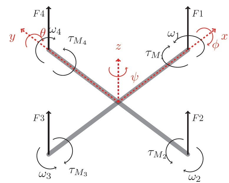
Even if we limit ourselves to considering just six degrees of freedom (three for position and three for orientation), the system is underactuated (one actuation from each rotor vs. six degrees of freedom) and is therefore not trivial to control. Fortunately, controllers exist that can ensure that actuation is realized by getting the four rotors to work in pairs, to balance the forces and torques of the system. With this approach, the quadcopter can be usefully modeled as a single rigid body with mass and inertia, by taking account of abstract force, gravity and actuation control torques. This model is depicted in Fig. 1.

III-C Mathematical Model

To generate the equations for the dynamics of our common quadcopter model [14], we first construct the rotational matrix to translate from an inertial (globally-fixed) reference frame to the body-fixed reference frame shown in Fig. 1. This matrix represents rotation about the $y$ axis ($\theta$), followed by rotation about the $x$ axis ($\phi$), and then rotation about the $z$ axis ($\psi$).

$$R=\begin{bmatrix}C_{\psi}C_{\theta}&C_{\psi}S_{\theta}C_{\phi}-S_{\psi}C_{\phi}&C_{\psi}S_{\theta}C_{\phi}+S_{\psi}S_{\phi}\\ S_{\psi}C_{\theta}&S_{\psi}S_{\theta}S_{\phi}+C_{\psi}C_{\theta}&S_{\psi}S_{\theta}C_{\phi}-C_{\psi}S_{\phi}\\ -S_{\theta}&C_{\theta}S_{\phi}&C_{\theta}C_{\phi}\end{bmatrix}$$ (1)

Here, $C$ , $S$ and $T$ refer to $cos$, $sin$, and $tan$, respectively. Next, summing forces on the quadcopter results in:

$$\sum F=m\bar{a}=G+RT$$ (2)

where $G$ is the force due to gravity, $R$ is the rotational matrix, and $T$ is the thrust from the motors. This expands to

$$\begin{bmatrix}\ddot{x}\\ \ddot{y}\\ \ddot{z}\end{bmatrix}=-g\begin{bmatrix}0\\ 0\\ 1\end{bmatrix}+\frac{T}{m}\begin{bmatrix}C_{\psi}S_{\theta}C_{\phi}+S_{\psi}S_{\phi}\\ S_{\psi}S_{\theta}C_{\phi}-C_{\psi}S_{\phi}\\ C_{\theta}C_{\phi}\end{bmatrix}$$ (3)

Finally, by summing moments about the center of mass, the equations for the dynamics for each of the rotational degrees of freedom can be determined as follows:

$$\begin{bmatrix}\ddot{\phi}\\ \ddot{\theta}\\ \ddot{\psi}\end{bmatrix}=\begin{bmatrix}0&\dot{\phi}C_{\phi}T_{\theta}+\dot{\theta}\frac{S_{\phi}}{C_{\theta}^{2}}&-\dot{\phi}S_{\phi}C_{\theta}+\dot{\theta}\frac{C_{\phi}}{C_{\theta}^{2}}\\ 0&-\dot{\phi}S_{\phi}&-\dot{\phi}C_{\phi}\\ 0&\dot{\phi}\frac{C_{\phi}}{C_{\theta}}+\dot{\phi}S_{\phi}\frac{T_{\theta}}{C_{\theta}}&-\dot{\phi}\frac{S_{\phi}}{C_{\theta}}+\dot{\theta}C_{\phi}\frac{T_{\theta}}{C_{\theta}}\end{bmatrix}\nu\\ \\ +W^{-1}_{\eta}\dot{\nu}$$ (4)

Where

$$\nu=\begin{bmatrix}p\\ q\\ r\end{bmatrix}=W_{\eta}\begin{bmatrix}\dot{\phi}\\ \dot{\theta}\\ \dot{\psi}\end{bmatrix}=\begin{bmatrix}1&0&-S_{\theta}\\ 0&C_{\phi}&C_{\theta}S_{p}hi\\ 0&-S_{\phi}&C_{\theta}C_{\phi}\end{bmatrix}\begin{bmatrix}\dot{\phi}\\ \dot{\theta}\\ \dot{\psi}\end{bmatrix}$$ (5)

$$\dot{\nu}=\begin{bmatrix}\left(I_{y}y-I_{z}z\right)\frac{qr}{I_{x}x}\\ \left(I_{z}z-I_{x}x\right)\frac{qr}{I_{y}y}\\ \left(I_{x}x-I_{y}y\right)\frac{qr}{I_{z}z}\\ -I_{r}\end{bmatrix}\begin{bmatrix}\frac{q}{I_{x}x}\\ \frac{-p}{I_{y}y}\\ 0\end{bmatrix}\omega_{\Gamma}+\begin{bmatrix}\frac{\tau_{\phi}}{I_{x}x}\\ \frac{\tau_{\theta}}{I_{y}y}\\ \frac{\tau_{\psi}}{I_{z}z}\end{bmatrix}$$ (6)

$$\begin{bmatrix}\tau_{\phi}\\ \tau_{\theta}\\ \tau_{\psi}\end{bmatrix}=\begin{bmatrix}lk\left(-\omega^{2}_{2}+\omega^{2}_{4}\right)\\ lk\left(-\omega^{2}_{1}+\omega^{2}_{3}\right)\\ \sum_{i=1}^{4}\tau_{M_{i}}\end{bmatrix}$$ (7)

Figure 1: Free body diagram of the quadcopter

III-D Acumen Model for Quadcopter

The equations derived earlier for the dynamics can be expressed in our core language as follows:

class QuadCopter(P,phi,theta,psi)
private
  g := 9.81;     m := 0.468;
  l := 0.225;    k := 2.98*10^(-6);
  b := 1.140*10^(-7);
  IM := 3.357*10^(-5);
  Ixx := 4.856*10^(-3);
  Iyy := 4.856*10^(-3);
  Izz := 8.801*10^(-3);
  Ax  := 0.25;  Ay  := 0.25;
  Az  := 0.25;
  w1 := 0;  w2:= 0;   w3 := 0;
  w4 := 0;  wT := 0;  f1 := 0;
  f2 := 0;  f3 := 0;  f4 := 0;
  TM1 := 0; TM2 := 0; T := 0;
  TM3 := 0; TM4 := 0;
  P’ := [0,0,0];    P’’ := [0,0,0];
  phi’ := 0; theta’ := 0; psi’ := 0;
  phi’’ := 0; theta’’ := 0; psi’’ := 0;
  p := 0; q := 0; r := 0; p’ := 0;
  q’ := 0; r’ := 0; Ch:=0; Sh:=0;
  Sp:=0; Cp:=0; St:=0; Ct:=0; Tt:=0
end
  T = k* (w1^2 + w2^2 + w3^2 + w4^2);
  f1 = k * w1^2; TM1 = b * w1^2;
  f2 = k * w2^2; TM2 = b * w2^2;
  f3 = k * w3^2; TM3 = b * w3^2;
  f4 = k * w4^2; TM4 = b * w4^2;
  wT = w1 - w2 + w3 - w4;

  Ch = cos(phi); Sh = sin(phi);
  Sp = sin(psi); Cp = cos(psi);
  St = sin(theta); Ct = cos(theta);
  Tt = tan(theta);

  P’’ = -g * [0,0,1] + T/m
   *[Cp*St*Ch+Sp*Sh,Sp*St*Ch-Cp*Sh,Ct*Ch]
   -1/m*[Ax*dot(P’,[1,0,0]),
         Ay*dot(P’,[0,1,0]),
         Az*dot(P’,[0,0,1])];
  p’ = (Iyy-Izz)*q*r/Ixx - IM*q/Ixx*wT
   + l*k*(w4^2 - w2^2)/Ixx;
  q’ = (Izz-Ixx)*p*r/Iyy-IM*(-p)/Iyy*wT
   + l*k*(w3^2 -w1^2)/Iyy;
  r’ = (Ixx - Iyy)*p*q/Izz  + b*(w1^2
   + w2^2 -w3^2 -w4^2)/Izz;
  phi’’ = (phi’*Ch*Tt+ theta’*Sh/Ct^2)*q
   + (-phi’*Sh*Ct+theta’*Ch/Ct^2)*r
   + (p’+q’*Sh*Tt+r’*Ch*Tt);
  theta’’ = (-phi’*Sh)*q + (-phi’*Ch)*r
   + (q’*Ch+r’*(-Sh));
  psi’’ = (phi’*Ch/Ct+phi’*Sh*Tt/Ct)*q
   + (-phi’*Sh/Ct+theta’*Ch*Tt/Ct)*r
   + (q’*Sh/Ct+r’*Ch/Ct);
end

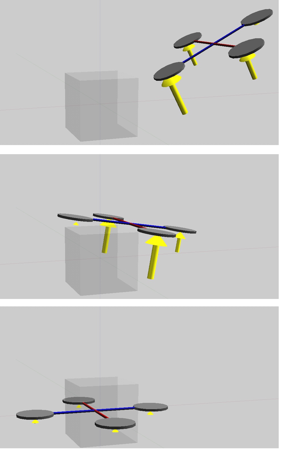
Fig. 2 presents snapshots of a 3D visualization of the quadcopter responding to a signal from a basic stabilizing controller [14]. This example shows that the Acumen core language can express models for complex mechatronic systems that are widely used in both research and education today.

Figure 2: The simulation results of the quadcopter model with PID control. Here the controller is bringing the quadcopter elevation, roll, pitch, and yaw to zero. Yellow arrows attached to each rotor indicate the thrust force generated by the rotors.

IV Lagrangian Modeling, and Why we Need it

Mathematical modeling of rigid body systems draws heavily on the field of classical mechanics. This field started in the 17th century with the introductions of Newton’s principles of motion and Newtonian modeling. Newton’s foundational work was followed by Lagrangian modeling in the 18th century, and Hamiltonian modeling in the 19th. Today, mechanical engineers make extensive use of the Lagrangian method when analyzing rigid body systems. It is therefore worthwhile to understand the process that engineers follow when using this method, and to consider the extent to which a modeling language can support this process.

The Newton method is focused on taking into consideration the forces and torques operating on a rigid body, and then computing the linear and angular accelerations of the center of mass of that rigid body. In general, this method consists of isolating the rigid body of interest in a free body diagram, selecting coordinate frame and summing forces and torques on the rigid body with respect to that frame, then using kinematics to express the linear and angular acceleration terms, before finally deriving the equations for the dynamics.

The Lagrangian method is based on the notion of action $L=T-V$, which is the difference between the kinetic $T$ and potential energy $V$. The Euler-Lagrange equation is itself a condition for ensuring that the total action in the system is stationary (constant). In Lagrangian modeling of physical systems, this condition should be seen as the analogy of the combined conditions $\Sigma F=ma$ and $\Sigma\tau=I\omega^{\prime\prime}$ in Newtonian mechanics. The Euler-Lagrange equation is as follows:

$$\forall i\in\{1...|q|)\},\frac{d}{dt}\left(\frac{\partial L}{\partial\dot{q_{i}}}\right)-\frac{\partial L}{\partial q_{i}}=Q$$ (8)

Using just this equation, the modeling process is reduced to specifying the kinetic and potential energy in the system. Part of the power of the method comes from the fact that this can be done using Cartesian, polar, spherical, or any other generalized coordinates. Compared to the classic Newtonian, force-vector based methods, the Euler-Lagrange equation is often a more direct specification of the dynamics.

The Lagrangian modeling process consists of four steps:

1. Start with a description of the components of the system, consisting of rigid bodies and joints. This description generally comes with a set of variable names which are collectively called called the generalized coordinates vector $q$. Intuitively, each variable represents a quantity corresponding to one of the degrees of freedom for the system. Usually, all of this information can be captured in an intuitive way in a free body diagram.

2. Determine the expression for the total kinetic and potential energy $T$ and $V$, respectively, of the system, in terms of the selected set of generalized coordinates $q$.

3. Identify and include any “external forces” $Q$ such as friction.

4. Substitute the values into the Euler-Lagrange equation (8) for the variables of second the derivative of $q$.

(a) Single

(b) Double

Figure 3: Free body diagram for single and double pendulums

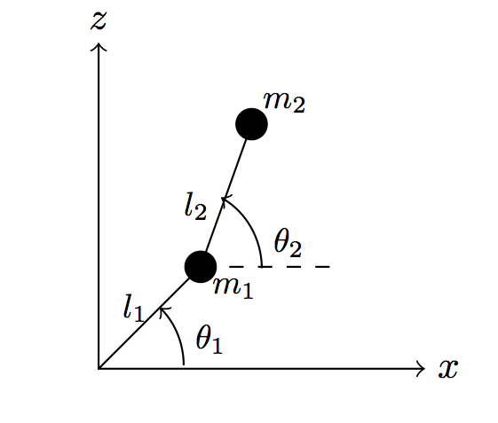
This process and its benefits can be illustrated with two small examples. The benefits apply whether or not the language supports directed or undirected equations. Figure 3 presents a free body diagram marked up with generalized coordinates ($\theta$ in one, and $\theta_{1},\theta_{2}$ in the other) for a single and a double pendulum system. First, we consider the single pendulum. A direct application of the angular part of Newton’s law gives us the following equation:

$$\ddot{\theta}=\frac{g}{l}\cos{\theta}$$ (9)

which is easily expressed in Acumen as follows:

class pendulum (l)
private
  theta := 0;theta’:=0;theta’’:=0;
  g:=9.81;
end
  theta’’ = g/l*cos(theta);
end

Lagrangian modeling can be applied to the single pendulum problem, but Newton’s method works well enough here. However, Lagrangian modeling does pay off for a double pendulum. It is instructive for language designers to recognize that such a seemingly small change in the complexity of the rigid body makes the model most of us learn about in high-school much more cumbersome than necessary. Whether or not this difficulty in modeling is due to weakness in Newtonian modeling or intrinsic complexity in this seemingly simple example is not obvious: The double pendulum is sophisticated enough to be widely used to model a human standing or walking [15], or a basic two-link robot such as the MIT-manus [16].

To derive a model for the double pendulum using Lagrangian modeling, we proceed as follows:

1. We take $q=(\theta_{1},\theta_{2})$. Here, because the Euler-Lagrange equation is parameterized by a generalized coordinate vector, we could have chosen to use Cartesian coordinates $(x,z)$ for each of the two points. Here we chose angles because they resemble what can be naturally measured and actuated at joints.

2. The kinetic and potential energies are defined as follows:

   $$T=\frac{1}{2}m_{1}v_{1}^{2}+\frac{1}{2}m_{2}v_{2}^{2}$$ (10)

   $$V=m_{1}gz_{1}+m_{2}gz_{2}$$ (11)

   where we have introduced shorthands for speeds $v_{1}^{2}=l_{1}^{2}\dot{\theta_{1}}^{2}$ and $v_{2}^{2}=v_{1}^{2}+\frac{1}{2}m_{2}(l_{1}^{2}\dot{\theta_{1}}^{2}+l_{2}^{2}\dot{\theta_{2}}^{2}+2l_{1}l_{2}\dot{\theta_{1}}\dot{\theta_{2}}\cos({\theta_{2}-\theta_{1}}))$, $z_{1}=l_{1}sin\theta_{1}$ and heights $z_{2}=z_{1}+l_{2}sin\theta_{2}$. Substituting these terms we get:

   $$T=\frac{1}{2}m_{1}(l_{1}\dot{\theta_{1}})^{2}\\ +\frac{1}{2}m_{2}(l_{1}^{2}\dot{\theta_{1}}^{2}+l_{2}^{2}\dot{\theta_{2}}^{2}+2l_{1}l_{2}\dot{\theta_{1}}\dot{\theta_{2}}\cos({\theta_{2}-\theta_{1}}))$$ (12)

   $$V=m_{1}gl_{1}\sin{\theta_{1}}+m_{2}gl_{2}\sin{\theta_{2}}+m_{2}gl_{1}\sin{\theta_{1}};$$ (13)

3. We assume frictionless joints, and so there are no external forces ($Q=0$).

4. By substitution and (manual) symbolic differentiation we get:

   $$(m_{1}+m_{2})l_{1}^{2}\ddot{\theta_{1}}+m_{2}l_{1}l_{2}\ddot{\theta_{2}}\cos{(\theta_{1}-\theta_{2})}\\ +m_{2}l_{1}l_{2}\dot{\theta_{1}}^{2}\sin({\theta_{1}-\theta_{2}})+m_{1}m_{2}gl_{1}\cos{\theta_{1}}=0$$ (14)

   $$m_{2}l_{2}^{2}\ddot{\theta_{2}}+m_{2}l_{1}l_{2}\ddot{\theta_{1}}\cos{(\theta_{1}-\theta_{2})}-\\ m_{2}l_{1}l_{2}\dot{\theta_{1}}^{2}\sin{(\theta_{1}-\theta_{2})}+m_{2}gl_{2}\cos{\theta_{2}}=0$$ (15)

   It is important to note in this case that, while these are ordinary differential equations (ODEs), they are not in the explicit form $X^{\prime}=E$. Rather, they are in implicit form, because the variable we are solving for ($X^{\prime}$) is not alone on one side of the equation. Using Gaussian elimination (under the assumption that the masses and length are strictly greater than zero), we get:

   $$\ddot{\theta_{1}}=m_{2}l_{2}(\ddot{\theta_{2}}\cos(\theta_{1}-\theta_{2})+\dot{\theta}_{2}^{2}\sin(\theta_{1}-\theta_{2})\\ +(m_{1}+m_{2})g\cos(\theta_{1}))/(-l_{1}(m_{1}+m_{2}))$$ (16)

   $$\ddot{\theta_{2}}=m_{2}l_{1}(\ddot{\theta_{1}}\cos(\theta_{1}-\theta_{2})-\dot{\theta}_{1}^{2}\sin(\theta_{1}-\theta_{2})\\ +m_{2}g\cos(\theta_{2}))/-l_{1}m_{2}$$ (17)

The following code shows these equations expressed in Acumen:

class double_pendulum (m_1, m_2, L_1, L_2)
private
  t_1 := 0; t_2 := 0;
  t_1’ := 0; t_2’ := 0;
  t_1’’ := 0; t_2’’ := 0;
  g:=9.81;
end
  t_1’’ =
   (m_2*L_2*(t_2’’*cos(t_1-t_2)
             +t_2’^2*sin(t_1-t_2))
    + (m_1+m_2)*g*cos(t_1))
   *(-1)/((m_1+m_2)*L_1);
  t_2’’ =
   (m_2*L_1*(t_1’’*cos(t_1-t_2)
             -t_1’^2*sin(t_1-t_2))
    +m_2*g*cos(t_2))
   *(-1)/(m_2*L_2);
end

Figure 4: The RiceWrist-S, with superimposed axes of rotation

V The RiceWrist-S Robot

Equipped with an understanding of Lagrangian modeling in the manner presented above, engineers model multi-link robots much more directly than with the Newtonian method. In this section we present one such case study using the RiceWrist-S research Robot.

V-A Background

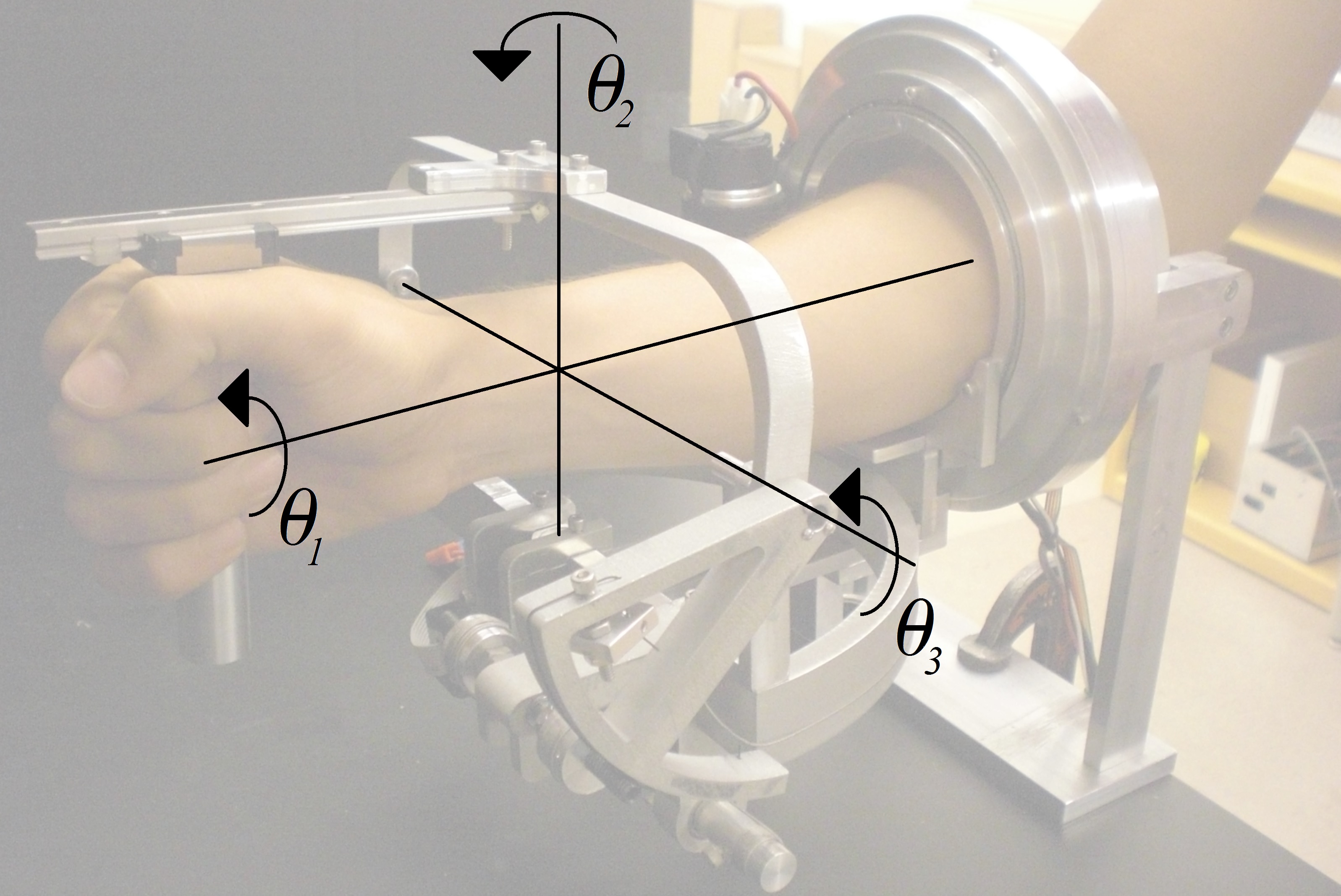
With an increasing number of individuals surviving once fatal injuries, the need for rehabilitation of damaged limbs is growing rapidly. Each year, approximately 795,000 people suffer a stroke in the United States, where stroke injuries are the leading cause of long-term disability. The RiceWrist-S [17] is an exoskeleton robot designed to assist in the rehabilitation of the wrist and forearm of stroke or spinal cord injury patients (Fig. 4). It consists of a revolute joint for each of the three degrees of freedom at the wrist. Because it has three rotational axes intersecting at one point, a good starting point to modeling it is the gimbal, a commonly studied mechanical device that also features several rotational axes intersecting at one point.

V-B Analytical Model

Figure 5: Free body diagram of the RiceWrist-S as a gimbal

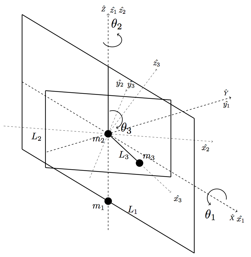
We can apply the Lagrangian modeling process to determine the dynamics of a gimbal as follows:

1. We take $q=(\theta_{1},\theta_{2},\theta_{3})$, where each of the angles corresponds to one of the three rotations possible in the RiceWrist-S (Fig. 5). We chose to represent the mass of the system as centralized to three locations, one at the origin, one at the bottom of the outermost ring, and one at the end of the third link. The masses in this figure correspond to the motors and handle depicted in Fig. 4.

2. To describe the energies concisely, it is convenient to use the following angular velocities of the gimbal frames in the kinetic energy terms, and the resulting heights for the potential energy terms:

   $$\begin{split}\omega_{1}=\,&\dot{\theta_{1}}\cdot\hat{x_{1}}\\ \end{split}$$ (18)

   $$\begin{split}\omega_{2}=\,&\dot{\theta_{1}}\cdot\hat{x_{1}}+\dot{\theta_{2}}\cdot\hat{z_{2}}\\ \end{split}$$ (19)

   $$\begin{split}\omega_{3}=\,&\dot{\theta_{1}}\cdot\hat{x_{1}}+\dot{\theta_{2}}\cdot\hat{z_{2}}+\dot{\theta_{3}}\cdot\hat{y_{3}}\\ \end{split}$$ (20)

   where $\hat{x_{i}}\hat{y_{i}}\hat{z_{i}}$ refers to the unit vector and coordinate frame about which these rotations occur, as shown in Fig. 5. Here, the $\omega_{i}$ terms correspond to the $m_{i}$ masses, and describe the angular velocities of that mass. Since this is a complex rotational system, many of the rotations do not occur in the coordinate frames of the respective gimbal. Therefore, in order to express each $\omega_{i}$ in terms of the same coordinate frame, we applied the following coordinate transforms:

   $$\begin{split}\omega_{1}=\,&\dot{\theta_{1}}\cdot\hat{x_{1}}\\ \end{split}$$ (21)

   $$\begin{split}\omega_{2}=\,&\dot{\theta_{1}}(\cos(\theta_{2})\cdot\hat{x_{2}}-\sin(\theta_{2})\cdot\hat{y_{2}})+\dot{\theta_{2}}\cdot\hat{z_{2}}\\ \end{split}$$ (22)

   $$\begin{split}\omega_{3}=\,&(\dot{\theta_{1}}(\cos(\theta_{2})\cos(\theta_{3}))+\dot{\theta_{2}}(-\sin(\theta_{3})))\cdot\hat{x_{3}}\\ &+(-\dot{\theta_{1}}\sin(\theta_{2})+\dot{\theta_{3}})\cdot\hat{y_{3}}+(-\dot{\theta_{1}}\sin(\theta_{3})\cos(\theta_{2})\\ &-\dot{\theta_{2}}\cos(\theta_{3}))\cdot\hat{z_{3}}\\ \end{split}$$ (23)

   Next, we express the heights above the predefined plane of zero potential energy (in Fig. 5, the $XY$ plane) of each of the masses $m_{1},m_{2},m_{3}$, respectively, as the following:

   $$\begin{split}h_{1}=\,&l_{2}\cos(\theta_{1})\\ \end{split}$$ (24)

   $$\begin{split}h_{2}=\,&0\\ \end{split}$$ (25)

   $$\begin{split}h_{3}=\,&l_{3}\sin(\theta_{1})\sin(\theta_{3})\\ \end{split}$$ (26)

   With this completed, the $T$ and $V$ terms can be quickly and easily defined. Since this is a rotational only system, $T$ is defined as the sum of the rotational energy terms, shown below:

   $$T=\frac{1}{2}(I_{1}\omega_{1}\cdot\ \omega_{1}+I_{2}\omega_{2}\cdot\omega_{2}+I_{3}\omega_{3}\cdot\omega_{3})$$ (27)

   Where $I_{i}$ is the rotational inertia corresponding to $\theta_{i}$, and $\omega_{i}$ is defined as above. And since there are no potential energy storage elements other than those caused by gravity, $V$ can be expressed with these heights:

   $$V=m_{1}gh_{1}+m_{2}gh_{2}+m_{3}gh_{3}\\ =-m_{1}gl_{2}\cos(\theta_{1})+m_{3}gl_{3}\sin(\theta_{1})\sin(\theta_{3})$$ (28)

3. Again, we assumed frictionless joints, so $Q=0$

4. After substitution and (manual) symbolic differentiation, we get an implicit set of equations. We solve these for $q^{\prime\prime}$ to get the equations of the systems dynamics.

   $$\frac{1}{2}\frac{d}{dt}\left(I_{1}\frac{\partial\omega_{1}\cdot\omega_{1}}{\partial\dot{\theta_{1}}}+I_{2}\frac{\partial\omega_{2}\cdot\omega_{2}}{\partial\dot{\theta_{1}}}+I_{3}\frac{\partial\omega_{3}\cdot\omega_{3}}{\partial\dot{\theta_{1}}}\right)+\\ m_{1}gl_{2}sin(\theta_{1})+m_{3}gl_{3}cos(\theta_{1})sin(\theta_{3})=0$$ (29)

   $$\frac{1}{2}\frac{d}{dt}\left(I_{2}\frac{\partial\omega_{2}\cdot\omega_{2}}{\partial\dot{\theta_{2}}}+I_{3}\frac{\partial\omega_{3}\cdot\omega_{3}}{\partial\dot{\theta_{2}}}\right)\\ -\frac{1}{2}\left(I_{2}\frac{\partial\omega_{2}\cdot\omega_{2}}{\partial{\theta_{2}}}+I_{3}\frac{\partial\omega_{3}\cdot\omega_{3}}{\partial{\theta_{2}}}\right)=0$$ (30)

   $$\frac{1}{2}\frac{d}{dt}\left(I_{3}\frac{\partial\omega_{3}\cdot\omega_{3}}{\partial\dot{\theta_{3}}}\right)-\frac{1}{2}\left(I_{3}\frac{\partial\omega_{3}\cdot\omega_{3}}{\partial{\theta_{3}}}\right)\\ -m_{3}gl_{3}sin(\theta_{1})cos(\theta_{3})=0$$ (31)

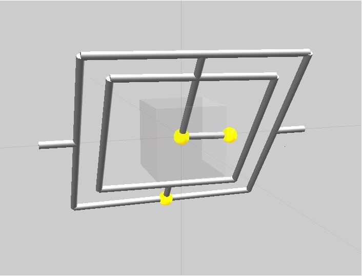
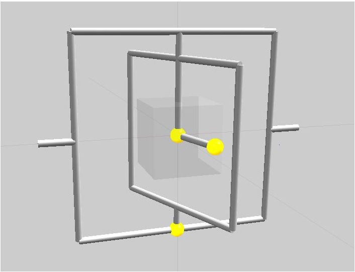
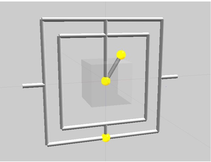
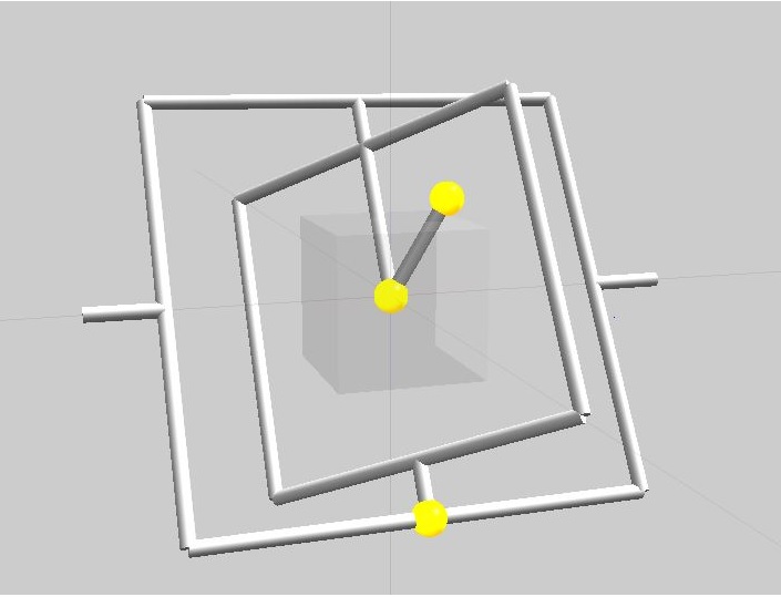
After computing the static partial derivatives, and the time derivatives, the resulting ODE’s are again, easy to express in Acumen. But they are too long to include here, as is the code [18]. What is significant about this situation is that these equations are linear in $\ddot{q}$ even though the system is also a non-linear differential equation (when we consider $q$, $\dot{q}$ and $\ddot{q}$). Because the system is linear in $\ddot{q}$, we can use standard Gaussian elimination to solve for $\ddot{q}$. This converts these implicit equations into an explicit form that is readily expressiable in Acumen. Fig. 6 shows the compound motion of the RW-S Gimbal model.

(a) Rotation about $\theta_{1}$

(b) Rotation about $\theta_{2}$

(c) Rotation about $\theta_{3}$

(d) Compound motion

Figure 6: RiceWrist-S modeled as Gimbal in Acumen.

VI Discussion

In this section, we step back to reflect on how to interpret this experience with expressing these various sytems in the small core language described at the outset of the paper.

VI-A The Role of a Core Language

At the highest level, Acumen can be seen as an untyped core formalism for a subset of hybrid systems modeling and simulation languages such as Modelica [7], Scicos [19] and Simcape [8]. It is easy to see that the CPS aspects that Acumen can express should be expressible by “larger” languages, but it is less clear what finding a weakspot in the expressivity of Acumen means for larger languages. In reasoning formally about expressivity limitations, it is beneficial that Acumen is untyped: any static type discpline adds restrictions, and whether or not such restrictions affects expressivity complicates such reasoning. While removing typing avoids this particular difficulty, it does not remove all the difficulties. Eventually, we expect to add a typing discpline to Acumen, but no particular direction has been decided at this time.

With several annual workshops related to its design and applications, Modelica is the most actively studied of the hybrid languages. It is a large language with many constructs. Acumen is small, with only a few features that are specific to hybrid systems. For example, Open Modelica’s parser [20] is roughly four times longer than the parser for Acumen. If Acumen can be seen as a subset of Modelica, it is reasonable to assume that the CPS aspects that Acumen can express can also be expressed in Modelica. At the same time, if features of CPS models are not easily expressed in Acumen, it is not immediately obvious wether or not they can be expressed in Modelica.

Another point that requires care in making the connection is the relation between Acumen’s notion of an object class and the abstraction mechanisms found in other languages. So far, our comparisons focus on issues relating to the expression and statement parts of these languages.

VI-B Supporting Lagrangian Modeling

The experience with the RiceWrist-S Robot suggests the need for Lagrangian modeling, which in turn points out to the need for two language features. The first feature is static partial derivatives. It has been observed elsewhere that the type of partial derivatives used in the Euler-Lagrange equation for rigid body dynamics can be removed at compile time (or “statically”) [5]. The pendulum examples show that CPS modeling languages should support the definition of explicit Langrangian models (requiring partial derivatives) because it simplifies the task of modeling rigid body systems, reducing the amount analysis, description, and algebraic manipulation the user would have to carry out.

Support for static partial derivatives in larger modeling and simulation tools seems sparse. While the Modelica standard (at least until recently) did not support partial derivatives, one implementation of Modelica, Dymola [21], does provide this support. Static partial derivatives are clearly an important feature to include in any DSL aiming to support CPS design.

In response to this observation, we have already introduced support for static partial derivatives in Acumen. The second language feature required (but is not sufficient without the first) to support Lagrangian modeling is implicit equations. The utility of implicit equations can be seen by reviewing the double pendulum example. Implicit equations are present in Modelica and Simscape. The construct does increase the reusability and flexibility of models, making composite models more concise. At this point it is not entirely clear to us how to best introduce implicit equations into a core language. To address this issue, we are currently implementing and experimenting with several different approaches from the literature. While different approaches may be better suited for different purposes (such as numerical precision, runtime performance, or others), our purpose behind this activity is to better understand how to position implicit equations in the context of other CPS DSL design decisions. A particularly interesting question here is whether this feature must be a primitive in the language or whether it can be treated as a conservative extension [22] of a core that does not include it.

VII Conclusions

This paper reports our most recent findings as we pursue an appropriate core language for CPS modeling and simulation. In particular, we present two examples. Our first example, a quadcopter, is significantly more sophisticated than any system considered in the first part. It shows that the core language proposed in Part I can express more sophisticated systems than was previously known. The second example, the RiceWrist-S, led us to understand the need for Lagrangian modeling, and as a result, provides us with concrete justification for introducing support for static partial derivatives. The most important lesson from this case study was that a DSL aimed at supporting CPS design should provide static partial derivatives and implicit equations. In order to ensure that we can push this line of investigation further, we have already developed a prototype of the former, and are working to realize the latter.

References

- [1] Taha Walid and Philippsen Roland. Modeling Basic Aspects of Cyber-Physical Systems. arXiv preprint arXiv:1303.2792, 2013.
- [2] Luca Carloni and Roberto Passerone and Alessandro Pinto and Alberto Sangiovanni-Vincentelli. Languages and tools for hybrid systems design. Foundations and Trends in Design Automation, 1(1):1–204, 2006.
- [3] Julien Bruneau, Charles Consel, Marcia O’Malley, Walid Taha, and Wail Masry Hannourah. Virtual Testing for Smart Buildings. In Proceedings of the 8th International Conference on Intelligent Environments (IE’12), Guanajuato’s, Mexico, 2012.
- [4] Jeff Jensen, Danica Chang, and Edward Lee. A Model-Based Design Methodology for Cyber-Physical Systems. In Proceedings of The First IEEE Workshop on Design, Modeling and Evaluation of Cyber Physical Systems (CyPhy’11), Istanbul, Turkey, July 2011.
- [5] Zhu Yun, Westbrook Edwin, Inoue Jun, Chapoutot Alexandre, Salama Cherif, Peralta Marisa, Martin Travis, Taha Walid, O’Malley Marcia, and Cartwright Robert. Mathematical equations as executable models of mechanical systems. In Proceedings of the 1st ACM/IEEE International Conference on Cyber-Physical Systems, pages 1–11. ACM, 2010.
- [6] E. Allen, D. Chase, J. Hallett, V. Luchangco, J.-W. Maessen, S. Ryu, G. L. Steele Jr., and S. Tobin-Hochstadt. The Fortress Language Specification. Technical report, Sun Microsystems, Inc., 2007.
- [7] Fritzson Peter and Bunus Peter. Modelica A General Object-Oriented Language for Continuous and Discrete-Event System Modeling and Simulation. In SS ’02: Proceedings of the 35th Annual Simulation Symposium, page 365, Washington, D.C., USA, 2002. IEEE Computer Society.
- [8] Inc. The Mathworks. Simscape documentation. http://www.mathworks.com/help/physmod/simscape/, 2013.
- [9] Walid Taha, Paul Brauner, Yingfu Zeng, Robert Cartrwright, Veronica Gaspes, Aaron Ames, and Alexandre Chapoutot. A Core Language for Executable Models of Cyber Physical Systems (Preliminary Report). In Proceedings of The Second International Workshop on Cyber-Physical Networking Systems (CPNS’12), Macau, China, June 2012.
- [10] Acumen website. www.acumen-language.org, 2010.
- [11] Walid Taha. Lecture notes on cyber-physical systems. Available online from www.effective-modeling.org/p/teaching.html, September 2012.
- [12] Taha Walid, Cartwright Robert, Philippsen Roland, and Zeng Yingfu. A First Course on Cyber Physical Systems. In 2013 Workshop on Embedded and Cyber-Physical Systems Education (WESE), Montreal, Canada, October 2013.
- [13] Taha Walid, Cartwright Robert, Philippsen Roland, and Zeng Yingfu. A First Course on Cyber Physical Systems. In Proceedings of the First Workshop on Cyber-Physical Systems Education (CPS-Ed 2013) at Cyber Physical Systems Week (CPSWeek 2013), Philadelphia, Pennsylvania, USA, April 2013. Available: http://cps-vo.org/group/edu/workshop/proceedings2013.
- [14] Teppo Luukkonen. Modelling and control of quadcopter, 2011. Aalto University, Espoo.
- [15] Pekarek David, Ames D. Aaron, and Marsden E. Jerrold. Discrete mechanics and optimal control applied to the compass gait biped. In Decision and Control, 2007 46th IEEE Conference on, pages 5376–5382. IEEE, 2007.
- [16] Neville Hogan, Hermano Igo Krebs, J Charnnarong, P Srikrishna, and Andre Sharon. MIT-MANUS: a workstation for manual therapy and training. i. In Robot and Human Communication, 1992. Proceedings., IEEE International Workshop on, pages 161–165. IEEE, 1992.
- [17] A.U Pehlivan, Lee Sangyoon, and M.K. O’Malley. Mechanical design of RiceWrist-S: A forearm-wrist exoskeleton for stroke and spinal cord injury rehabilitation. In Biomedical Robotics and Biomechatronics (BioRob), 2012 4th IEEE RAS EMBS International Conference on, pages 1573–1578, 2012.
- [18] Yingfu Zeng, Chad Rose, and Walid Taha. RiceWrist-S: Gimbal model. available online from. http://bit.ly/RiceWristGimbal, 2013.
- [19] Ramine Nikoukhah. Modeling hybrid systems in Scicos: a case study. In Proceedings of the 25th IASTED international conference on Modeling, indentification, and control, MIC’06. ACTA Press, 2006.
- [20] Modelica. parser. https://www.modelica.org/tools/parser.
- [21] H. Olsson, H. Tummescheit, and H. Elmqvist. Using automatic differentiation for partial derivatives of functions in Modelica. In Proceedings of Modelica, pages 105–112, Hamburg, Germany , March 2005.
- [22] Matthias Felleisen. On the expressive power of programming languages. In Science of Computer Programming, pages 134–151. Springer-Verlag, 1990.