Realizing $\mathcal{PT}$-symmetric non-Hermiticity with ultra-cold atoms and Hermitian multi-well potentials

Abstract

We discuss the possibility of realizing a non-Hermitian, i. e. an open two-well system of ultra-cold atoms by enclosing it with additional time-dependent wells that serve as particle reservoirs. With the appropriate design of the additional wells $\mathcal{PT}$-symmetric currents can be induced to and from the inner wells, which support stable solutions. We show that interaction in the mean-field limit does not destroy this property. As a first method we use a simplified variational ansatz leading to a discrete nonlinear Schrödinger equation. A more accurate and more general variational ansatz is then used to confirm the results.

I Introduction

Since the first realization of $\mathcal{PT}$-symmetric gain and loss in optical wave guides Rüter et al. (2010) much effort has been made to realize analogous systems in various fields of physics, e. g. lasers Chong et al. (2011), electronics Schindler et al. (2011), microwave cavities Bittner et al. (2012), and to make use of new effects arising from nonlinearity, viz. the Kerr nonlinearity in optical wave guides Ramezani et al. (2010). $\mathcal{PT}$ symmetry originates from quantum mechanics and stands for a combined action of parity and time-reversal. Despite the non-Hermiticity of $\mathcal{PT}$-symmetric Hamiltonians, in a certain range of parameters entirely real eigenvalue spectra exist Bender and Boettcher (1998). Due to a formal analogy between quantum mechanics and electromagnetism, the formulation of $\mathcal{PT}$ symmetry has spread to those systems, leading to the above mentioned realizations. However, the experimental verification in a genuine quantum system has not been achieved so far.

In a $\mathcal{PT}$-symmetric system there is a balanced gain and loss of probability density (or electromagnetic field in analogue systems). According to a proposal in Klaiman et al. (2008) such a quantum mechanical system could be realized with a Bose-Einstein condensate (BEC) in a double-well potential where particles are injected into one well and removed from the other. Indeed, it could be shown that the system is ideally suited for a first-experimental observation of $\mathcal{PT}$ symmetry in a quantum system Dast et al. (2013). There is progress in coupling two BECs and at the same time eject particles Shin et al. (2005), but an actual realization of $\mathcal{PT}$ symmetry using a BEC is still missing.

On the other hand much theoretical work has been done on $\mathcal{PT}$-symmetric BECs, including the proof of existence of stable states of interacting systems Cartarius and Wunner (2012), a microscopic treatment based on the Bose-Hubbard model Graefe et al. (2008), and a thorough investigation on dynamics of stable and unstable regimes Haag et al. (2014). In contrast to injecting and removing particles from a double-well potential, one could think of a double-well included in a tilted optical lattice, with an incoming and outgoing transport of particles, so called Wannier-Stark systems Zenesini et al. (2008); Elsen et al. (2011). These incoming and outgoing particle currents could in principle serve as the necessary currents for realizing a $\mathcal{PT}$-symmetric system.

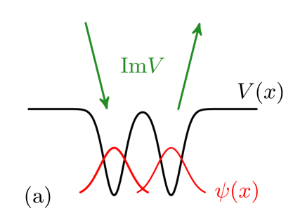
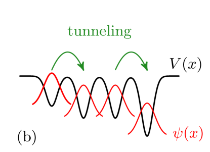
Figure 1: (a) Two-mode model with an imaginary potential $V$, where – in this case – particles are removed from the left well and injected into the right. (b) Such a system could be realized by coupling two additional wells to the system, where the tunneling currents to and from the outer wells are used as an implementation of the imaginary potential. The outer wells act as (limited) particle reservoirs and have to be chosen time-dependent.

In a recent Rapid Communication Kreibich et al. (2013) we followed the simplest approach to this idea, namely to couple two additional wells to the double well potential (see Fig. 1), and use the arising currents as a theoretical realization of $\mathcal{PT}$ symmetry in a quantum mechanical system. We showed that for a specific time-dependent choice of the well depths and coupling strengths of the additional wells, the inner wells behave exactly as the wells of a $\mathcal{PT}$-symmetric two-well system, thus serving as a possible experimental realization.

It is the purpose of this paper investigate more deeply our approach, especially for the case of interacting atoms, and to formulate a more accurate method to confirm the results. In Sec. II we derive the few-mode model or discrete nonlinear Schrödinger equation (DNLSE) from the Gross-Pitaevskii equation (GPE) using a simple variational ansatz, where each well is populated by a single time-independent Gaussian function. The results are applied in Sec. III to show that a Hermitian four-mode model can be chosen such that the middle wells behave exactly as the wells of the $\mathcal{PT}$-symmetric two-mode model. This is exemplified for some parameters. In Sec. IV we use an extended variational ansatz for the realization of $\mathcal{PT}$ symmetry. Still one Gaussian function per well is used, but each Gaussian function is fully dynamical in its parameters, thus giving a more accurate description of the system. The method is compared with the simply Gaussian ansatz. In Sec. V we conclude our work.

II From the Gross-Pitaevskii equation to a few-mode model

In this section we apply the steps that lead from the GPE, which describes the dynamics of a BEC at absolute zero temperature, to a DNLSE or few-mode-model. At first we presents our ansatz and calculate the necessary integrals. To derive the equations of motion (EOM) in a Schrödinger form we use the method of symmetric orthogonalization. In Sec. III the results are used and applied to different scenarios.

II.1 Simplified variational ansatz

We start with the well-known GPE,

$$\mathrm{i}\hbar\partial_{t}\psi({\bm{r}},t)=\left[-\frac{\hbar^{2}}{2m}\Delta+V({\bm{r}})+g\left|\psi({\bm{r}},t)\right|^{2}\right]\psi({\bm{r}},t).$$ (1)

The interaction strength is given by $g=4\pi\hbar^{2}Na/m$ with the s-wave scattering length $a$ and particle number $N$. For the external multi-well potential $V({\bm{r}})$ we use a Gaussian profile for each well,

$$V({\bm{r}})=\sum\limits_{k=1}^{{N_{\text{w}}}}V^{k}\exp\left[-\frac{2x^{2}}{w_{x}^{2}}-\frac{2y^{2}}{w_{y}^{2}}-\frac{2(z-s_{z}^{k})^{2}}{w_{z}^{2}}\right],$$ (2)

with a total number of ${N_{\text{w}}}$ wells. Each well $k$ has the potential depth $V^{k}<0$ and is displaced along the $z$-direction by $s_{z}^{k}$. Such a potential could, e. g., be created experimentally by the method presented in Henderson et al. (2009).

There is various work on how to transform the GPE (1) into a DNLSE Trombettoni and Smerzi (2001); Smerzi and Trombettoni (2003) by integrating out the spatial degrees of freedom. In general, an ansatz of the form

$$\psi({\bm{r}},t)=\sum\limits_{k}d^{k}(t)g^{k}({\bm{r}}),$$ (3)

is used, where $d^{k}(t)$ is the (complex) amplitude and $g^{k}({\bm{r}})$ the localized wave function in well $k$. Usually, a set of Wannier functions is applied Bloch et al. (2008). In this work [Sec. III], we use a single Gaussian function for each well. With this ansatz we can derive analytical formulae for the matrix elements of the DNLSE or few-mode model, and thus open an easy way to actually compute the localized wave functions by a simple energy minimization process. In Sec. IV we extend the variational ansatz to obtain more accurate results.

The simplified variational ansatz is given by the superposition of ${N_{\text{G}}}$ Gaussian functions, one for each well, ${N_{\text{w}}}={N_{\text{G}}}$, with

$$g^{k}({\bm{r}})=\,{\mathrm{e}}^{-A_{x}^{k}x^{2}-A_{y}^{k}y^{2}-A_{z}^{k}(z-q_{z}^{k})^{2}}.$$ (4)

The parameters $A_{x}^{k},A_{y}^{k},A_{z}^{k}\in\mathbbm{R}$ describe the width of each Gaussian function in each direction, and $q_{z}^{k}\in\mathbbm{R}$ the displacement along the $z$-direction. We treat these parameters in this section as time-independent. The time-dependence of the wave function comes from the amplitude $d^{k}(t)$ in Eq. (3).

We insert ansatz (3) into the GPE $\mathrm{i}\hbar\partial_{t}\psi=\hat{H}\psi$, multiply from the left with $(g^{l})^{*}$, and integrate over $\mathbbm{R}^{3}$. Then, we are left with

$$\mathrm{i}\hbar{\bm{\mathrm{K}}}\dot{{\bm{d}}}={\bm{\mathrm{H}}}{\bm{d}}.$$ (5)

Here, the amplitudes $d^{k}$ are written as a vector ${\bm{d}}=(d^{1},\dots,d^{N_{\text{G}}})^{\text{T}}\in\mathbbm{C}^{N_{\text{G}}}$. The matrix ${\bm{\mathrm{K}}}$ describes the overlap, and ${\bm{\mathrm{H}}}$ the Hamiltonian matrix elements. They are given by the integrals (see Sec. II.2 for their explicit calculation)

$$K_{lk} =\left\langle g^{l}\middle|g^{k}\right\rangle,$$ (6a)

$$H_{lk} =\left\langle\left.\vphantom{\hat{H}g^{k}}g^{l}\right|\hat{H}\left|\vphantom{\hat{H}g^{l}}g^{k}\right.\right\rangle.$$ (6b)

Our aim is to derive EOM for the amplitudes in a Schrödinger form, i. e. $\mathrm{i}\hbar\dot{{\bm{d}}}_{\text{eff}}={\bm{\mathrm{H}}}_{\text{eff}}{\bm{d}}_{\text{eff}}$, with possibly modified amplitudes and matrix elements. Equation (5) would be of that form if ${\bm{\mathrm{K}}}$ was proportional to the identity matrix. Since the Gaussian functions $g^{k}$ are non-orthogonal this is not the case. For that reason, we perform a symmetric orthogonalization in Sec. II.3.

II.2 Evaluation of the integrals

The occurring integrals in Eqs. (6) are solely based on the Gaussian integral

$$\int\limits_{-\infty}^{\infty}\!\mathrm{d}x\,x^{n}\,{\mathrm{e}}^{-Ax^{2}+px} =\frac{\partial^{n}}{\partial p^{n}}\int\limits_{-\infty}^{\infty}\!\mathrm{d}x\,\,{\mathrm{e}}^{-Ax^{2}+px}$$

$$=\frac{\partial^{n}}{\partial p^{n}}\sqrt{\frac{\pi}{A}}\,{\mathrm{e}}^{p^{2}/4A},\qquad\operatorname{Re}A>0.$$ (7)

For convenience we define the abbreviations

$$A_{\alpha}^{kl} =A_{\alpha}^{k}+(A_{\alpha}^{l})^{*},\qquad\alpha=x,y,z,$$ (8a)

$$\kappa_{\alpha}^{kl} =A_{\alpha}^{k}(A_{\alpha}^{l})^{*}/A_{\alpha}^{kl},$$ (8b)

$$\beta_{\alpha}^{kl} =\sqrt{\frac{A_{\alpha}^{kl}w_{\alpha}^{2}}{A_{\alpha}^{kl}w_{\alpha}^{2}+2}},$$ (8c)

$$c^{kl} =\,{\mathrm{e}}^{-\kappa_{z}^{kl}(q_{z}^{k}-q_{z}^{l})^{2}}.$$ (8d)

The integrals of ${\bm{\mathrm{K}}}$ can now easily be calculated with Eq. (II.2) for the case $n=0$, the result is

$$K_{lk}=\sqrt{\frac{\pi}{A_{x}^{kl}}}\sqrt{\frac{\pi}{A_{y}^{kl}}}\sqrt{\frac{\pi}{A_{z}^{kl}}}c^{kl}.$$ (9)

For the calculation of the Hamiltonian matrix ${\bm{\mathrm{H}}}$, we separate it into a kinetic term ${\bm{\mathrm{T}}}$, an external potential term ${\bm{\mathrm{V}}}$, and an interaction term ${\bm{\mathrm{W}}}$.

For the kinetic term we need integrals of the form shown in Eq. (II.2) with $n=2$ and we obtain

$$T_{lk}=K_{lk}\left[\kappa_{x}^{kl}+\kappa_{y}^{kl}+\kappa_{z}^{kl}-2(\kappa_{z}^{kl})^{2}(q_{z}^{k}-q_{z}^{l})^{2}\right].$$ (10)

To calculate the integrals necessary for the external potential, the parameters $A$ and $p$ in Eq. (II.2) are shifted by the parameters of the external potential. The result is

$$V_{lk}=K_{lk}\beta_{x}^{kl}\beta_{y}^{kl}\beta_{z}^{kl}\sum\limits_{m}V^{m}\\ \times\exp\left\{-\frac{2\left[A_{z}^{k}(s_{z}^{m}-q_{z}^{k})+(A_{z}^{l})^{*}(s_{z}^{m}-q_{z}^{l})\right]^{2}}{A_{z}^{kl}(A_{z}^{kl}w_{z}^{2}+2)}\right\}.$$ (11)

Since the operator of the interaction potential ${\bm{\mathrm{W}}}$ is nonlinear, its matrix elements depend on the amplitudes $d^{k}$. With the standard Gaussian integral we obtain

$$W_{lk}=\sum\limits_{i,j}\tilde{W}_{lkji}(d^{j})^{*}d^{i},$$ (12)

where we defined the four-rank tensor

$$\tilde{W}_{lkji}=\frac{4\pi\hbar^{2}Na}{m}\sqrt{\frac{\pi}{A_{x}^{ijkl}}}\sqrt{\frac{\pi}{A_{y}^{ijkl}}}\sqrt{\frac{\pi}{A_{z}^{ijkl}}}\\ \times\exp\left[-\frac{A_{z}^{i}(A_{z}^{j})^{*}(q_{z}^{i}-q_{z}^{j})^{2}+A_{z}^{i}(A_{z}^{l})^{*}(q_{z}^{i}-q_{z}^{l})^{2}}{A_{z}^{ijkl}}\right]\\ \times\exp\left[-\frac{A_{z}^{k}(A_{z}^{j})^{*}(q_{z}^{k}-q_{z}^{j})^{2}+A_{z}^{k}(A_{z}^{l})^{*}(q_{z}^{k}-q_{z}^{l})^{2}}{A_{z}^{ijkl}}\right]\\ \times\exp\left[-\frac{A_{z}^{i}A_{z}^{k}(q_{z}^{i}-q_{z}^{k})^{2}+(A_{z}^{j})^{*}(A_{z}^{l})^{*}(q_{z}^{j}-q_{z}^{l})^{2}}{A_{z}^{ijkl}}\right]$$ (13)

and the new abbreviations

$$A_{\alpha}^{ijkl}=A_{\alpha}^{ij}+A_{\alpha}^{kl},\qquad\alpha=x,y,z.$$ (14)

II.3 Symmetric orthogonalization

We calculated all necessary integrals for setting up the EOMs (5), which are not of the form of a Schrödinger equation (cf. Sec. II.1). To achieve this, we now transform the EOM into a Schrödinger form with the method of symmetric orthogonalization Löwdin (1950): Since ${\bm{\mathrm{K}}}$ is Hermitian there exists a unitary transformation ${\bm{\mathrm{U}}}$ such that ${\bm{\mathrm{D}}}={\bm{\mathrm{U}}}{\bm{\mathrm{K}}}{\bm{\mathrm{U}}}^{\dagger}$ is diagonal with real entries. Then we can construct the Hermitian matrix

$${\bm{\mathrm{X}}}={\bm{\mathrm{U}}}^{\dagger}{\bm{\mathrm{D}}}^{-1/2}{\bm{\mathrm{U}}}.$$ (15)

This matrix has the properties that ${\bm{\mathrm{X}}}{\bm{\mathrm{K}}}{\bm{\mathrm{X}}}=\mathbbm{1}$, and furthermore, if ${\bm{\mathrm{H}}}$ is Hermitian, so is ${\bm{\mathrm{X}}}{\bm{\mathrm{H}}}{\bm{\mathrm{X}}}$. Now, we can use this matrix to transform Eq. (5) to

$$\mathrm{i}\hbar({\bm{\mathrm{X}}}{\bm{\mathrm{K}}}{\bm{\mathrm{X}}})({\bm{\mathrm{X}}}^{-1}\dot{{\bm{d}}})=({\bm{\mathrm{X}}}{\bm{\mathrm{H}}}{\bm{\mathrm{X}}})({\bm{\mathrm{X}}}^{-1}{\bm{d}}).$$ (16)

With the definitions ${\bm{d}}_{\text{eff}}={\bm{\mathrm{X}}}^{-1}{\bm{d}}$ and ${\bm{\mathrm{H}}}_{\text{eff}}={\bm{\mathrm{X}}}{\bm{\mathrm{H}}}{\bm{\mathrm{X}}}$, and the above property of ${\bm{\mathrm{X}}}$ we arrive at the EOM for ${\bm{d}}_{\text{eff}}$ in Schrödinger form

$$\mathrm{i}\hbar\dot{{\bm{d}}}_{\text{eff}}={\bm{\mathrm{H}}}_{\text{eff}}{\bm{d}}_{\text{eff}}$$ (17)

with a Hermitian Hamiltonian matrix ${\bm{\mathrm{H}}}_{\text{eff}}$ (if ${\bm{\mathrm{H}}}$ is Hermitian). We note, that the normalization condition for the wave function $\psi$ transforms as

$$1 \stackrel{{\scriptstyle!}}{{=}}\int\!\mathrm{d}^{3}r\,\left|\psi\right|^{2}={\bm{d}}^{\dagger}{\bm{\mathrm{K}}}{\bm{d}}=({\bm{\mathrm{X}}}^{-1}{\bm{d}})^{\dagger}({\bm{\mathrm{X}}}{\bm{\mathrm{K}}}{\bm{\mathrm{X}}})({\bm{\mathrm{X}}}^{-1}{\bm{d}})$$

$$={\bm{d}}_{\text{eff}}^{\dagger}{\bm{d}}_{\text{eff}}.$$ (18)

II.4 Application of symmetric orthogonalization and nearest-neighbor approximation

By means of symmetric orthogonalization we can transform the EOM (5) into a Schrödinger form since we know ${\bm{\mathrm{K}}}$ analytically. Without any further approximations the analytical expressions can become quite complicated. At this point, we introduce as usual the nearest neighbor approximation to obtain analytical and simple approximate expressions for ${\bm{\mathrm{X}}}$ and ${\bm{\mathrm{H}}}_{\text{eff}}$.

The structure of the matrix elements $K_{lk}$ [see Eq. (9)] allows for a natural approximation since the function $c^{kl}$ drops exponentially with increasing distance of wells $\left|k-l\right|$. We say a term is of order $n$ when $\left|k-l\right|=n$. As an approximation we only consider terms up to order $n=1$. Hence, we have ${\bm{\mathrm{K}}}={\bm{\mathrm{K}}}^{(0)}+{\bm{\mathrm{K}}}^{(1)}$ with

$$K_{lk}^{(0)}=\left(\frac{\pi}{2}\right)^{3/2}\frac{\delta_{kl}}{\sqrt{A_{x,R}^{k}A_{y,R}^{k}A_{z,R}^{k}}}$$ (19)

and

$$K_{lk}^{(1)}=\sqrt{\frac{\pi}{A_{x}^{kl}}}\sqrt{\frac{\pi}{A_{y}^{kl}}}\sqrt{\frac{\pi}{A_{z}^{kl}}}c^{kl}\left(\delta_{k,l+1}+\delta_{k+1,l}\right),$$ (20)

where $A_{\alpha,R}^{k}=\operatorname{Re}A_{\alpha}^{k}$, and – for later use – $A_{\alpha,I}^{k}=\operatorname{Im}A_{\alpha}^{k}$.

Using this expansion, we calculate the zeroth order of ${\bm{\mathrm{X}}}$ by the requirement ${\bm{\mathrm{X}}}^{(0)}{\bm{\mathrm{K}}}^{(0)}{\bm{\mathrm{X}}}^{(0)}=\mathbbm{1}$. We obtain

$$X_{lk}^{(0)}=\left(\frac{2}{\pi}\right)^{3/4}\sqrt[4]{A_{x,R}^{k}A_{y,R}^{k}A_{z,R}^{k}}\delta_{kl}.$$ (21)

To calculate the first order we start with

$$\left({\bm{\mathrm{X}}}^{(0)}+{\bm{\mathrm{X}}}^{(1)}\right)\left({\bm{\mathrm{K}}}^{(0)}+{\bm{\mathrm{K}}}^{(1)}\right)\left({\bm{\mathrm{X}}}^{(0)}+{\bm{\mathrm{X}}}^{(1)}\right)=\mathbbm{1},$$ (22)

ignore second order terms, insert the known quantities, and solve for ${\bm{\mathrm{X}}}^{(1)}$, which yields

$$X_{lk}^{(1)}=-\left(\frac{8}{\pi}\right)^{3/4}\frac{c^{kl}}{\sqrt{A_{x}^{kl}}\sqrt{A_{y}^{kl}}\sqrt{A_{z}^{kl}}}\left(\delta_{k,l+1}+\delta_{k+1,l}\right)\\ \times\frac{\sqrt{A_{x,R}^{k}A_{y,R}^{k}A_{z,R}^{k}A_{x,R}^{l}A_{y,R}^{l}A_{z,R}^{l}}}{\sqrt[4]{A_{x,R}^{k}A_{y,R}^{k}A_{z,R}^{k}}+\sqrt[4]{A_{x,R}^{l}A_{y,R}^{l}A_{z,R}^{l}}}.$$ (23)

Now we are able to calculate analytical approximations for the transformed Hamiltonian ${\bm{\mathrm{H}}}_{\text{eff}}$. We observe that for the linear parts, i. e. the kinetic and external potential part, the matrix elements of ${\bm{\mathrm{H}}}$ are proportional to ${\bm{\mathrm{K}}}$, so we can write $H_{lk}^{\text{lin}}=K_{lk}h_{lk}^{\text{lin}}$ [cf. Eqs. (10) and (11)]. Thus, the orders of ${\bm{\mathrm{H}}}^{\text{lin}}$ are given by the orders of ${\bm{\mathrm{K}}}$. Therefore, for the zeroth order transformed Hamiltonian we obtain

$$H_{{\text{eff}},lk}^{{\text{lin}},(0)}=\sum\limits_{m,n}X_{lm}^{(0)}K_{mn}^{(0)}X_{nk}^{(0)}h_{mn}^{\text{lin}}=h_{kk}^{\text{lin}}\delta_{kl}.$$ (24)

The zeroth order contributes to the linear diagonal elements of ${\bm{\mathrm{H}}}_{\text{eff}}^{\text{lin}}$, so they can be identified with the onsite energy $E_{k}=h_{kk}^{\text{lin}}$. With Eqs. (10) and (11) we can write

$$E_{k}=\frac{\hbar^{2}}{2m}\left(A_{x,R}^{k}+A_{y,R}^{k}+A_{z,R}^{k}\right)\\ +V^{k}\beta_{x}^{kk}\beta_{y}^{kk}\beta_{z}^{kk}\exp\left[-2(\beta_{z}^{kk})^{2}(s_{z}^{k}-q_{z}^{k})^{2}/w_{z}^{2}\right],$$ (25)

where we considered only the term with $m=k$ in the sum in Eq. (11) to be consistent with zeroth order.

The first order terms of ${\bm{\mathrm{H}}}_{\text{eff}}^{\text{lin}}$ are given by the first order terms of the expression

$$({\bm{\mathrm{X}}}^{(0)}+{\bm{\mathrm{X}}}^{(1)})({\bm{\mathrm{H}}}^{{\text{lin}},(0)}+{\bm{\mathrm{H}}}^{{\text{lin}},(1)})({\bm{\mathrm{X}}}^{(0)}+{\bm{\mathrm{X}}}^{(1)}),$$ (26)

which gives, after inserting all known quantities,

$$H_{{\text{eff}},lk}^{{\text{lin}},(1)}= -2\sqrt{2}\frac{\sqrt{A_{x,R}^{k}A_{y,R}^{k}A_{z,R}^{k}A_{x,R}^{l}A_{y,R}^{l}A_{z,R}^{l}}}{\sqrt[4]{A_{x,R}^{k}A_{y,R}^{k}A_{z,R}^{k}}+\sqrt[4]{A_{x,R}^{l}A_{y,R}^{l}A_{z,R}^{l}}}$$

$$\times\left(\frac{E_{k}-h_{lk}}{\sqrt[4]{A_{x,R}^{k}A_{y,R}^{k}A_{z,R}^{k}}}+\frac{E_{l}-h_{lk}}{\sqrt[4]{A_{x,R}^{l}A_{y,R}^{l}A_{z,R}^{l}}}\right)$$

$$\times\frac{c^{kl}}{\sqrt{A_{x}^{kl}}\sqrt{A_{y}^{kl}}\sqrt{A_{z}^{kl}}}\left(\delta_{k,l+1}+\delta_{k+1,l}\right).$$ (27)

These elements can be identified as the tunneling elements of the few-mode model, i. e. $J_{lk}=-H_{{\text{eff}},lk}^{{\text{lin}},(1)}$, since they are the super- and sub-diagonal entries. The quantity $h_{lk}^{\text{lin}}$ is given by Eqs. (10) and (11), where in $v_{lk}$ we only consider nearest-neighbor contributions,

$$v_{lk}=\beta_{x}^{kl}\beta_{y}^{kl}\beta_{z}^{kl}\\ \times\Biggl{(}V^{k}\exp\left\{-\frac{2\left[A_{z}^{k}(s_{z}^{k}-q_{z}^{k})+(A_{z}^{l})^{*}(s_{z}^{k}-q_{z}^{l})\right]^{2}}{A_{z}^{kl}(A_{z}^{kl}w_{z}^{2}+2)}\right\}\\ +V^{l}\exp\left\{-\frac{2\left[A_{z}^{k}(s_{z}^{l}-q_{z}^{k})+(A_{z}^{l})^{*}(s_{z}^{l}-q_{z}^{l})\right]^{2}}{A_{z}^{kl}(A_{z}^{kl}w_{z}^{2}+2)}\right\}\Biggr{)}.$$ (28)

So far we have calculated the matrix elements of the linear transformed Hamiltonian ${\bm{\mathrm{H}}}_{\text{eff}}^{\text{lin}}$. We now turn our attention to the interaction part. Since the operator ${\bm{\mathrm{W}}}$ is nonlinear and depends on the amplitudes $d^{k}$, they must be transformed, too. For the transformed operator, we obtain

$$W_{{\text{eff}},lk} =\sum\limits_{i,j,m,n,p,q}X_{lm}\tilde{W}_{mnji}X_{nk}(X_{jp}d_{\text{eff}}^{p})^{*}(X_{iq}d_{\text{eff}}^{q})$$

$$=\sum\limits_{p,q}\underbrace{\sum\limits_{i,j,m,n}X_{lm}X_{pj}\tilde{W}_{mnji}X_{nk}X_{iq}}_{\equiv\tilde{W}_{{\text{eff}},lkpq}}(d_{\text{eff}}^{p})^{*}d_{\text{eff}}^{q}.$$ (29)

For the interaction term, we only consider onsite-elements, i. e. elements with $i=j=k=l$ in $\tilde{W}_{lkji}$, since mainly these terms contribute to the interaction part. For the transformed four-rank tensor, we then obtain

$$\tilde{W}_{{\text{eff}},kkkk}=\frac{4\hbar^{2}Na}{\sqrt{\pi}m}\sqrt{A_{x,R}^{k}A_{y,R}^{k}A_{z,R}^{k}}.$$ (30)

These elements are the nonlinear coupling constants, $c_{k}=\tilde{W}_{{\text{eff}},kkkk}$. The whole action of the transformed Hamiltonian then reads

$$W_{{\text{eff}},lk}=c_{k}|d^{k}|^{2}\delta_{kl}.$$ (31)

We have all necessary matrix-elements in nearest-neighbor approximation. Using this knowledge we can calculate these elements from the Gaussian variational approach, or – vice verse – determine the parameters of the realistic potential (2) by knowing the matrix elements. As an application this is done in Sec. III. The parameters $A_{\alpha}^{k}$ and $q_{z}^{k}$ can be computed by minimizing the mean-field energy of the system for a given initial condition with

$$E_{\text{mf}}=\sum\limits_{k,l}(d^{l})^{*}\left(T_{lk}+V_{lk}\right)d^{k}\\ +\frac{1}{2}\sum\limits_{i,j,k,l}(d^{l})^{*}d^{k}W_{lkji}(d^{j})^{*}d^{i}.$$ (32)

For this minimization, all parameters $A_{\alpha}^{k}$, $q_{z}^{k}$ and $d^{k}$ have to be varied with the norm constraint (II.3), which is computationally much cheaper than a grid calculation. The results of this section could also be used to calculate the parameters of the Bose-Hubbard model.

Now that we have all matrix elements, we can begin our actual investigation of a realization of a non-Hermitian system, first by means of few-mode models. In the following we will adopt the usual notation and write for the discrete wave function $\psi_{k}$ instead of $d^{k}$.

III Few-Mode models

III.1 Equivalence of the two- and four-mode models

We now return to the idea mentioned in the introduction and sketched in Fig. 1, i. e. the embedding of a non-Hermitian double-well with a closed four-well structure. Before analyzing the possibility of realizing a non-Hermitian system with a Hermitian model, we discuss the basic properties of the non-Hermitian two-mode model, which is given by

$${\bm{\mathrm{H}}}_{2}=\begin{pmatrix}E_{1}+c_{1}\left|\psi_{1}\right|^{2}&-J_{12}\\ -J_{12}&E_{2}+c_{2}\left|\psi_{2}\right|^{2}\end{pmatrix}$$ (33)

with complex onsite energies $E_{k}\in\mathbbm{C}$, which make the Hamiltonian non-Hermitian. This system has intensively been investigated in Graefe (2012). The time derivatives of the observables, that is particle number $n_{k}=\psi_{k}^{*}\psi_{k}$ and particle current $j_{kl}=\mathrm{i}J_{kl}(\psi_{k}\psi_{l}^{*}-\psi_{k}^{*}\psi_{l})$, can be easily calculated, which gives

$$\partial_{t}n_{1} =-j_{12}+2n_{1}\operatorname{Im}E_{1},$$ (34a)

$$\partial_{t}n_{2} =j_{12}+2n_{2}\operatorname{Im}E_{2},$$ (34b)

$$\partial_{t}j_{12} =2J_{12}^{2}(n_{1}-n_{2})+(\operatorname{Im}E_{1}+\operatorname{Im}E_{2})j_{12}$$

$$\quad+J_{12}(\operatorname{Re}E_{1}-\operatorname{Re}E_{2}+c_{1}n_{1}-c_{2}n_{2})C_{12},$$ (34c)

$$\partial_{t}C_{12} =(\operatorname{Im}E_{1}+\operatorname{Im}E_{2})C_{12}$$

$$\quad-(\operatorname{Re}E_{1}-\operatorname{Re}E_{2}+c_{1}n_{1}-c_{2}n_{2})\tilde{j}_{12},$$ (34d)

where we defined $C_{kl}=\psi_{k}\psi_{l}+\psi_{k}^{*}\psi_{l}^{*}$ and $\tilde{j}_{kl}=\mathrm{i}(\psi_{k}\psi_{l}^{*}-\psi_{k}^{*}\psi_{l})=j_{12}/J_{12}$. In Eqs. (34a) and (34b) we see that the imaginary parts of the onsite energies act as additional sources or sinks to the particle flow, the quantities $j_{e1}=2n_{1}\operatorname{Im}E_{1}$ and $j_{e2}=-2n_{2}\operatorname{Im}E_{2}$ can be identified as currents to and from the environment, thus, this Hamiltonian describes an open quantum system.

The general solutions for the nonlinear model (33) are calculated in Graefe (2012). For convinience we only discuss the results of the linear, i. e. non-interacting case ($c_{1}=c_{2}=0$). Then, the eigenvalues are given by

$$E_{\pm}=\frac{E_{1}+E_{2}}{2}\pm\sqrt{J_{12}^{2}+\frac{(E_{1}-E_{2})^{2}}{2}}.$$ (35)

Requirement for $\mathcal{PT}$ symmetry leads to the condition $E_{1}=E_{2}^{*}$, which is for instance fulfilled by $E_{1}=\mathrm{i}\Gamma$ and $E_{2}=-\mathrm{i}\Gamma$, a situation with balanced gain and loss. Then, the eigenvalues are $E_{\pm}=\sqrt{J_{12}^{2}-\Gamma^{2}}$. For $\Gamma<J_{12}$ they are real, whereas for $\Gamma>J_{12}$ the $\mathcal{PT}$ symmetry is broken and the eigenvalues are purely imaginary.

It is now our main purpose to investigate whether the behavior of the non-Hermitian two-mode model (33) can be described by a Hermitian four-mode model, which is given by

$${\bm{\mathrm{H}}}_{4}(t)=\begin{pmatrix}E_{0}(t)&-J_{01}(t)&0&0\\ -J_{01}(t)&E_{1}&-J_{12}&0\\ 0&-J_{12}&E_{2}&-J_{23}(t)\\ 0&0&-J_{23}(t)&E_{3}(t)\end{pmatrix}\\ +\operatorname{diag}\left(c_{0}\left|\psi_{0}\right|^{2},c_{1}\left|\psi_{1}\right|^{2},c_{2}\left|\psi_{2}\right|^{2},c_{3}\left|\psi_{3}\right|^{2}\right).$$ (36)

Two additional wells are coupled to the system, they act as a particle reservoir for the inner wells. The onsite energies and tunneling elements of the outer wells may be time-dependent. Since this model shall be Hermitian, the onsite energies are real, $E_{k}\in\mathbbm{R}$.

To derive a relationship between the two- and four-mode model we calculate the time derivatives of the same observables as in the two-mode model, which yields

$$\partial_{t}n_{1} =j_{01}-j_{12},$$ (37a)

$$\partial_{t}n_{2} =j_{12}-j_{23},$$ (37b)

$$\partial_{t}j_{12} =2J_{12}^{2}\left(n_{1}-n_{2}\right)-J_{12}\left(J_{01}C_{02}-J_{23}C_{13}\right)$$

$$\quad+J_{12}\left(E_{1}-E_{2}+c_{1}n_{1}-c_{2}n_{2}\right)C_{12},$$ (37c)

$$\partial_{t}C_{12} =J_{01}\tilde{j}_{02}-J_{23}\tilde{j}_{13}-\left(E_{1}-E_{2}+c_{1}n_{1}-c_{2}n_{2}\right)\tilde{j}_{12}.$$ (37d)

Comparing with Eqs. (34) we find that for the two-mode model the following condition must hold,

$$\operatorname{Im}E_{1}=-\operatorname{Im}E_{2}\Rightarrow E_{1}=E_{2}^{*}.$$ (38)

This means that only the $\mathcal{PT}$-symmetric two-mode model, as discussed above, may be simulated by the four-mode model. From now on we write $E_{1}=\mathrm{i}\Gamma$ and $E_{2}=-\mathrm{i}\Gamma$ with $\Gamma\in\mathbbm{R}$. Furthermore, the real parts of the onsite energies $E_{1}$ and $E_{2}$ and the coupling element $J_{12}$ have to agree between the two models. We are then left with the following conditions,

$$j_{01} =2\Gamma n_{1},$$ (39a)

$$j_{23} =2\Gamma n_{2},$$ (39b)

$$0 =J_{01}C_{02}-J_{23}C_{13},$$ (39c)

$$0 =J_{01}\tilde{j}_{02}-J_{23}\tilde{j}_{13}.$$ (39d)

To summarize at this point, if these conditions are fulfilled at every time, the two middle wells of the Hermitian four-mode model behave exactly as the wells of the $\mathcal{PT}$-symmetric two-mode model. These four conditions seem to be independent, but we shall see in App. A that Eq. (39d) follows if Eqs. (39a)–(39c) are fulfilled.

We now have to make clear that these conditions can indeed be fulfilled by giving suitable time-dependencies to the elements of the four-mode Hamiltonian. Equation (39c) can simply be fulfilled by choosing

$$J_{01}(t)=dC_{13}(t), J_{23}(t)=dC_{02}(t),$$ (40)

where $d\neq 0$ is a real, time-independent quantity. The tunneling elements are then time-dependent. With $J_{01}$ and $J_{23}$ determined there are no free parameters left to fulfill Eqs. (39a) and (39b). Instead, we can set the time-derivatives of these equations with the help of the remaining onsite energies $E_{0}$ and $E_{3}$. We calculate the time-derivatives of $j_{01}$ and $j_{23}$ using the Schrödinger equation, which yields

$$\partial_{t}j_{01} =\left(\partial_{t}J_{01}\right)\tilde{j}_{01}+2J_{01}^{2}\left(n_{0}-n_{1}\right)+J_{01}J_{12}C_{02}$$

$$\quad+J_{01}\left(E_{0}-E_{1}+c_{0}n_{0}-c_{1}n_{1}\right)C_{01}$$

$$\stackrel{{\scriptstyle!}}{{=}}\partial_{t}j_{01}^{\text{tar}},$$ (41a)

$$\partial_{t}j_{23} =\left(\partial_{t}J_{23}\right)\tilde{j}_{23}+2J_{23}^{2}\left(n_{2}-n_{3}\right)-J_{23}J_{12}C_{13}$$

$$\quad+J_{23}\left(E_{2}-E_{3}+c_{2}n_{2}-c_{3}n_{3}\right)C_{23}$$

$$\stackrel{{\scriptstyle!}}{{=}}\partial_{t}j_{23}^{\text{tar}},$$ (41b)

with the target currents determined by Eqs. (39a) and (39b). The time derivatives of the tunneling elements $J_{01}$ and $J_{23}$ are given by

$$\partial_{t}J_{01} =d\partial_{t}C_{13}$$

$$=d\left(J_{01}\tilde{j}_{03}+J_{12}\tilde{j}_{23}-J_{23}\tilde{j}_{12}\right)$$

$$\quad+d\left(E_{3}-E_{1}+c_{3}n_{3}-c_{1}n_{1}\right)\tilde{j}_{13},$$ (42a)

$$\partial_{t}J_{23} =d\partial_{t}C_{02}$$

$$=d\left(J_{01}\tilde{j}_{12}-J_{12}\tilde{j}_{01}-J_{23}\tilde{j}_{03}\right)$$

$$\quad+d\left(E_{2}-E_{0}+c_{2}n_{2}-c_{0}n_{0}\right)\tilde{j}_{02}.$$ (42b)

Inserting this into Eqs. (41), the onsite energies $E_{0}$ and $E_{3}$ are determined by a linear set of equations,

$$\begin{pmatrix}C_{01}C_{13}&\tilde{j}_{01}\tilde{j}_{13}\\ -\tilde{j}_{02}\tilde{j}_{23}&-C_{02}C_{23}\end{pmatrix}\begin{pmatrix}E_{0}\\ E_{3}\end{pmatrix}=\begin{pmatrix}v_{0}\\ v_{3}\end{pmatrix},$$ (43)

with the entries

$$v_{0} =\partial_{t}j_{01}^{\text{tar}}/d-J_{12}\tilde{j}_{23}-d\left(C_{13}\tilde{j}_{03}-C_{02}\tilde{j}_{12}\right)\tilde{j}_{01}$$

$$\quad-2dC_{13}^{2}\left(n_{0}-n_{1}\right)-J_{12}C_{02}C_{13}$$

$$\quad-\left(c_{3}n_{3}-c_{1}n_{1}\right)\tilde{j}_{01}\tilde{j}_{13}-\left(c_{0}n_{0}-c_{1}n_{1}\right)C_{01}C_{13},$$ (44a)

$$v_{3} =\partial_{t}j_{23}^{\text{tar}}/d+J_{12}\tilde{j}_{01}-d\left(C_{13}\tilde{j}_{12}-C_{02}\tilde{j}_{03}\right)\tilde{j}_{23}$$

$$\quad-2dC_{02}^{2}\left(n_{2}-n_{3}\right)+J_{12}C_{02}C_{13}$$

$$\quad-\left(c_{2}n_{2}-c_{0}n_{0}\right)\tilde{j}_{02}\tilde{j}_{23}-\left(c_{2}n_{2}-c_{3}n_{3}\right)C_{02}C_{23},$$ (44b)

where we set $E_{1}=E_{2}=0$, since – as discussed above – the real parts of these elements have to agree between the two- and four-mode model.

We have to note that by means of the onsite energies $E_{0}$ and $E_{3}$ we do not fix the currents, but their time-derivatives. For this reason the initial probabilities and currents have to be chosen such that they fulfill the conditions (39). In the following section we apply these results to obtain solutions for different starting conditions.

III.2 Results

Before presenting our results we give the necessary initial conditions. We insert the definition of the particle current and the solutions for the tunneling elements (40) into the two Eqs. (39a) and (39b) and express everything in terms of the wave function $\psi_{k}$. We are allowed to choose the global phase of the initial wave function, so we choose $\psi_{2}^{I}=0$. We assume the real parts $\psi_{0}^{R}$ and $\psi_{3}^{R}$ to be arbitrary but fixed. We are left with (after simple rearrangement)

$$\psi_{3}^{I} =\frac{\Gamma}{2d\psi_{0}^{R}},$$ (45a)

$$\psi_{0}^{I} =\frac{\psi_{0}^{R}\psi_{1}^{I}}{\psi_{1}^{R}}-\frac{\Gamma n_{1}}{2d\psi_{1}^{R}\left(\psi_{1}^{R}\psi_{3}^{R}+\psi_{1}^{I}\psi_{3}^{I}\right)}.$$ (45b)

Now, the wave function $\psi_{k}$ fulfills the necessary conditions and with the time-dependencies of the matrix elements from Sec. III.1 we can simulate the $\mathcal{PT}$-symmetric two-mode model.

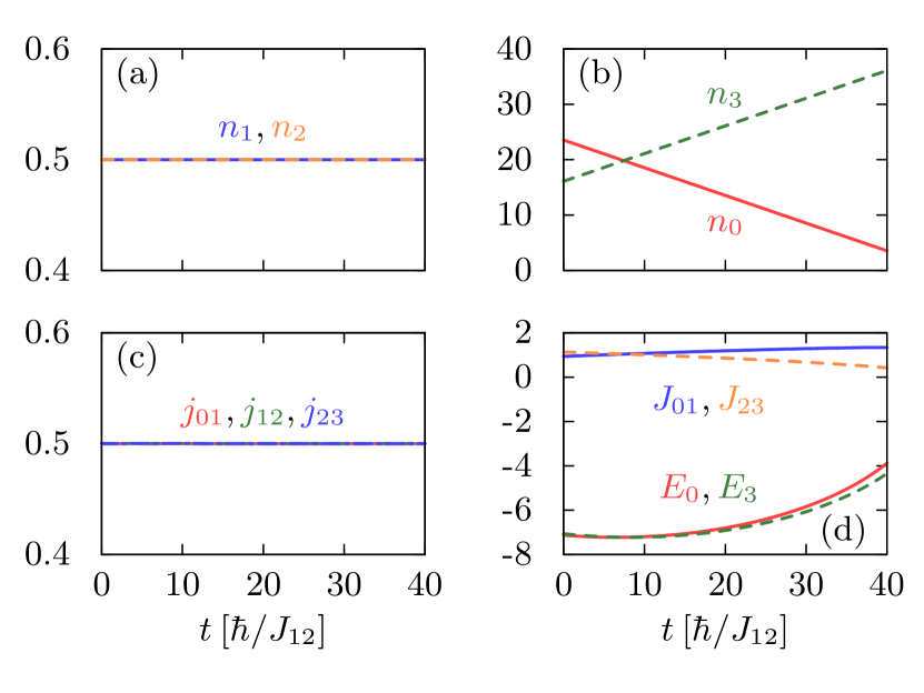
Figure 2: Realization of a stationary $\mathcal{PT}$-symmetric solution within the four-mode model. (a) Particles numbers in well 1 (solid) and well 2 (dashed), both equal to $1/2$. (b) Particle numbers in well 0 (solid) and well 3 (dashed). (c) Particle currents $j_{01}$ (solid), $j_{12}$ (dashed) and $j_{23}$ (dash-dotted) in units of $J_{12}/\hbar$. (d) Tunneling elements $J_{01}$ (solid), $J_{23}$ (dashed), and onsite energies $E_{0}$ (solid), $E_{3}$ (dashed), in units of $J_{12}$.

First we consider a stationary solution in the non-interacting case [cf. Eq. (35)] for $\Gamma/J_{12}=0.5$. Fig. 2 shows the results. As expected the particle numbers in the two middle wells are both equal and constant in time (with normalization $n_{1}+n_{2}=1$), as well as the particle currents. For this reason, the number of particles decreases (left well) or increases linearly (right well), with the slope $\dot{n}_{0}=-\Gamma/\hbar$ and $\dot{n}_{3}=\Gamma/\hbar$, respectively. The matrix elements of the four-mode model vary slightly in time. Thus, we have shown that the conditions (39) can be fulfilled for a finite time.

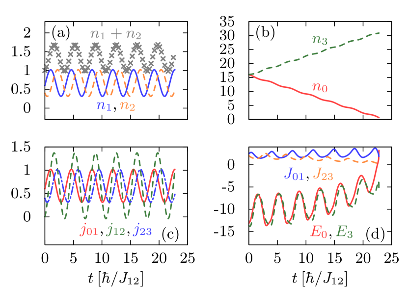
Figure 3: Same as Fig. 2, but for oscillatory dynamics. Additionally, the added number of particles $n_{1}+n_{2}$ is plotted as crosses in (a). As the particle number in the reservoir well 0 decreases and gets close to zero, the conditions cannot be fulfilled anymore and the simulation breaks down.

As a second example we prepare a non-stationary solution at $t=0$, with $\psi_{1}(0)=\sqrt{0.6}$ and $\psi_{2}(0)=\sqrt{0.4}$ (see Fig. 3). In this case the particle numbers in the two middle wells oscillate in time with a phase difference $\Delta\phi<\pi$ leading to a non-constant added number of particles, which is a typical feature of $\mathcal{PT}$-symmetric systems. Since well 0 acts as a particle reservoir the number of particles decreases and gets close to zero up to the point where the linear system of equations (43) cannot be fulfilled anymore (determinant of coefficient matrix equals zero). This shows that the time available for a simulation of $\mathcal{PT}$ symmetry with a reservoir is limited. The matrix elements in this case show a quasi-oscillatory behavior.

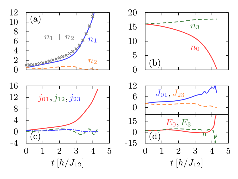
Figure 4: Same as Fig. 2, but for the interacting case ($c=-1$), which leads to a collapsing dynamics, indicating a change of stability. The reservoir is emptying in a short time domain such that the time available for $\mathcal{PT}$ symmetry is quite short.

Next, we consider a system with attractive interaction $c=-1$. In such a system it is known that the ground state changes its stability in an additional bifurcation (for repulsive interaction, the excited state changes its stability) Haag et al. (2014). This phenomenon is highly correlated to the occurrence of self-trapping states. In our example $2\times 2$ system [Eq. (33)] the ground state is already unstable for the given interaction strength, so that the ground state with a small perturbation is expected to collapse. The calculation is shown in Fig. 4. The particle number $n_{1}$ increases exponentially, which marks the beginning of collapse. To support the exponential increase, the particle number in the reservoir $n_{0}$ is decreasing exponentially, so that the simulation breaks down after a quite short time interval. The matrix elements now show a rather complex time-dependency.

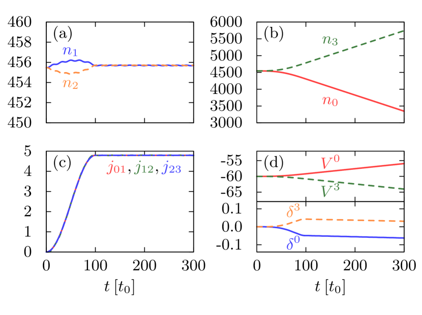
Figure 5: Same as Fig. 2, but for an adiabatic current ramp ($\Gamma_{\text{f}}/J_{12}=0.5$, $t_{\text{f}}/t_{0}=60$) for realistic parameters of the external potential. Instead of the matrix elements, in (d) we show the parameters of the potential, $\delta^{k}$ marks the displacement from equidistant potential wells. There is a total number of particles of $N=10^{4}$. See text for units.

As the last example we calculate an experimentally more realistic scenario. Up to now – as mentioned above – we had to start with appropriate wave functions in order to obtain $\mathcal{PT}$ symmetry. This is nearly impossible in an experiment. To overcome this, we use an adiabatic change of the $\mathcal{PT}$ parameter from zero to its target value. We start at the ground state of the Hermitian four-mode model (with $\Gamma=0$) and increase $\Gamma$ to its target value $\Gamma_{\text{f}}$. If this change is slow enough, we arrive approximately at the $\mathcal{PT}$-symmetric ground state. The specific time dependence we use is $\Gamma(t)=\Gamma_{\text{f}}[1-\cos(\pi t/t_{\text{f}})]/2$ for $t\in[0,t_{\text{f}}]$.

In the following we simulate a condensate of $N=10^{5}$ atoms of ^87Rb. We use units based on the potential width in $z$-direction, $w_{z}$, which we set $w_{z}=$1\text{\,}\mathrm{\SIUnitSymbolMicro m}$$. The basic unity of energy is $E_{0}=\hbar^{2}/mw_{z}^{2}$, which yields $E_{0}/h=$116\text{\,}\mathrm{Hz}$$. The basic unit of time is $t_{0}=mw_{z}^{2}/\hbar=$1.37\text{\,}\mathrm{ms}$$. The wells have widths of $w_{x}=w_{y}=4w_{z}=$4\text{\,}\mathrm{\SIUnitSymbolMicro m}$$, and are initially positioned equidistantly with a distance of $1.8w_{z}=$1.8\text{\,}\mathrm{\SIUnitSymbolMicro m}$$. The potential depths are given by $V^{0}=V^{3}=-60E_{0}$ and $V^{1}=V^{2}=-45E_{0}$. We use a scattering length of $a=2.83a_{\text{B}}$ with $a_{\text{B}}$ being the Bohr radius.

We calculate the adiabatic ramp for $\Gamma_{\text{f}}/J_{12}=0.5$ and $t_{\text{f}}/t_{0}=60$. The results are shown in Fig. 5. The total particle number and currents are scaled to a particle number of $N=10^{5}$, the currents are given in units of $1/t_{0}$, the potential depths in units of $E_{0}$. Instead of the positions of the potential wells we plot the difference of the position from its initial value, $\delta^{k}=s_{z}^{k}-s_{z}^{k}(t=0)$. By means of the relations derived in Sec. II we can transform from the calculated matrix elements to parameters of the external potential.

After time $t_{\text{f}}$ an approximate $\mathcal{PT}$-symmetric state is obtained. This can be seen by the constant number of particles in the middle wells, despite an increasing and decreasing number in wells 3 and 0, respectively, which is a clear sign of $\mathcal{PT}$ symmetry, also in a possible experiment. The potential depths of the outer wells have to be adjusted in a simple way, the positions vary within a few percent of the distance of the wells. This shows that the simple four-mode model can be used to describe a realistic scenario and to obtain the necessary parameters of the external potential.

We have applied our results from Sec. III.1 to different initial conditions and system parameters and have shown that it is indeed possible to realize a $\mathcal{PT}$-symmetric system with a Hermitian four-mode model. In the following Section we investigate this scenario in the framework of the GPE and a variational ansatz with Gaussian functions. In particular we verify that the results from this section agree.

IV Variational ansatz with Gaussian functions

IV.1 Variational ansatz and equations of motion

After the simple approach in the previous section we now investigate the possible realization in the framework of the GPE with an extended variational ansatz. We use a superposition of Gaussian functions, where – in contrast to the simpler approach of Sec. II.1 – all variational parameters are considered as time-dependent,

$$\psi=\sum\limits_{k}\,{\mathrm{e}}^{-({\bm{r}}-{\bm{q}}^{k})^{\text{T}}{\bm{\mathrm{A}}}^{k}({\bm{r}}-{\bm{q}}^{k})+\mathrm{i}{\bm{p}}^{k}({\bm{r}}-{\bm{q}}^{k})-\gamma^{k}}.$$ (46)

The matrices ${\bm{\mathrm{A}}}^{k}=\operatorname{diag}(A_{x}^{k},A_{y}^{k},A_{z}^{k})\in\mathbbm{C}^{3\times 3}$ describe the width of each Gaussian function in each direction, the vectors ${\bm{q}}^{k}=(0,0,q_{z}^{k})^{\text{T}}\in\mathbbm{R}^{3}$ and ${\bm{p}}^{k}=(0,0,p_{z}^{k})^{\text{T}}\in\mathbbm{R}^{3}$ the position and momentum, respectively, and the scalar quantities $\gamma^{k}\in\mathbbm{C}$ the amplitude and phase. This variational ansatz can describe a much richer dynamics than ansatz (4) and thus we expect more accurate results.

The equations of motion follow from the time-dependent variational principle in the formulation of McLachlan McLachlan (1964), which states that the quantity

$$I=||\mathrm{i}\hbar\phi-\hat{H}\psi||^{2}$$ (47)

shall be minimized with respect to $\phi$ and $\phi=\dot{\psi}$ is set afterwards. Details of the necessary calculation can be found in Ref. Eichler et al. (2012), where the ansatz (46) has been used to study the collision of anisotropic solitons in a BEC. The EOM are given by

$$\mathrm{i}\hbar\sum\limits_{k}\left\langle\frac{\partial\psi}{\partial z_{l}}\middle|\frac{\partial\psi}{\partial z_{k}}\right\rangle\dot{z}_{k}=\left\langle\left.\vphantom{\hat{H}\psi}\frac{\partial\psi}{\partial z_{l}}\right|\hat{H}\left|\vphantom{\hat{H}\frac{\partial\psi}{\partial z_{l}}}\psi\right.\right\rangle,$$ (48)

where ${\bm{z}}=(A_{x}^{1},\dots,\gamma^{N_{\text{G}}})^{\text{T}}$ is the vector of all variational parameters. Stationary solutions are given by fixed points of (48), whereas the dynamics can be calculated by integrating Eq. (48) with a numerical integrator.

In Sec. III we started our considerations by calculating the time-derivatives of the observables. In the case of the continuous GPE with a non-Hermitian potential this leads to the modified equation of continuity

$$\dot{\rho}+\operatorname{div}{\bm{j}}=2\rho\operatorname{Im}V,$$ (49)

with $\rho=\left|\psi\right|^{2}$ and ${\bm{j}}=\hbar(\psi^{*}\bm{\nabla}\psi-\psi\bm{\nabla}\psi^{*})/2m\mathrm{i}$. The imaginary part of the potential acts as an additional source or sink to the probability flow. Instead of adjusting the matrix elements, we need to adjust the parameters of the external potential. Since Eq. (49) is given on the whole space $\mathbbm{R}^{3}$, one would need to change the external potential at every point in space, which is not manageable, neither in theory nor in an experiment.

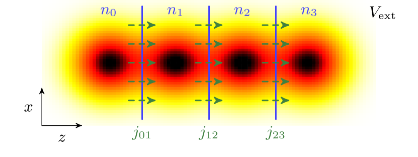
Figure 6: External potential $V_{\text{ext}}$; the darker, the deeper the potential. The wells are separated into regions by walls at positions right in the middle between two minima. The integral over $\left|\psi\right|^{2}$ in a region $k$ is the particle number $n_{k}$; the current through a wall is denoted by $j_{k,k+1}$. See text for exact definitions. With this separation we obtain a formulation analogous to the four-mode model (Sec. III).

To overcome this problem we use the results of Sec. III as a roadmap for this continuous system. For that, we separate the individual wells by walls between two minima of the potential at positions $z_{k}=(s_{z}^{k}+s_{z}^{k+1})/2$ for $k=1,2,3$, $z_{0}\to-\infty$ and $z_{4}\to\infty$ (see Fig. 6). To obtain time derivatives of discrete observables as in the few-mode model, we integrate the continuity equation for the Hermitian four-well potential over a volume

$$V^{k}=\{(x,y,z)^{\text{T}}|-\infty<x,y<\infty,z_{k-1}<z<z_{k}\}.$$ (50)

This yields

$$\partial_{t}\iiint\limits_{V^{k}}\mathrm{d}^{3}r\,\rho =-\iiint\limits_{V^{k}}\mathrm{d}^{3}r\,\operatorname{div}{\bm{j}}$$

$$=-\iint\limits_{\partial V^{k}}\mathrm{d}{\bm{A}}\cdot{\bm{j}}.$$ (51)

The integral on the left-hand side can be interpreted as the number of particles in well $k$. On the right-hand side we used Gauss’s theorem. The surface integrals goes over a box, where the areas in the $x$-$z$- and $y$-$z$-plane go to infinity. We assume the current ${\bm{j}}$ to also vanish at infinity, so only the integral over the two surfaces in the $x$-$y$-plane contribute. Thus, we can write

$$\partial_{t}n_{k}=-\int\limits_{-\infty}^{\infty}\mathrm{d}x\int\limits_{-\infty}^{\infty}\mathrm{d}y\,\left[j_{z}(x,y,z_{k})-j_{z}(x,y,z_{k-1})\right].$$ (52)

The integral over the $z$-component of ${\bm{j}}$ evaluated at $z_{k}$ represents the current from well $k$ to $k+1$, which we write as $j_{k,k+1}$, for $z_{k-1}$ this represents the current from well $k-1$ to $k$, $j_{k-1,k}$. We finally obtain from the continuity equation

$$\partial_{t}n_{k}=j_{k-1,k}-j_{k,k+1},$$ (53)

where $j_{-1,0}=j_{3,4}=0$.

Therefore, with Eq. (53) we have an analogous equation as for the few-mode-model (37). We can use the same method to realize a $\mathcal{PT}$-symmetric system. At every time step of the numerical integration of the equations of motion (48) we vary the parameters of the external potential such that the observables show the desired behavior. This is done via a nonlinear root search, in contrast to the analytical solutions of Sec. III.1. In Sec. III.2 we showed that the positions of the outer wells barely needed to be adjusted. As a simplification we only vary the depths of the outer wells $V^{0}$, $V^{3}$ and demand the outer currents $j_{01}$, $j_{23}$ to reach the desired values. We are left with a two-dimensional root search. In the following section we determine the realization of $\mathcal{PT}$ symmetry within the GPE and compare the results with those of the few-mode-model.

IV.2 Results and comparison with few-mode models

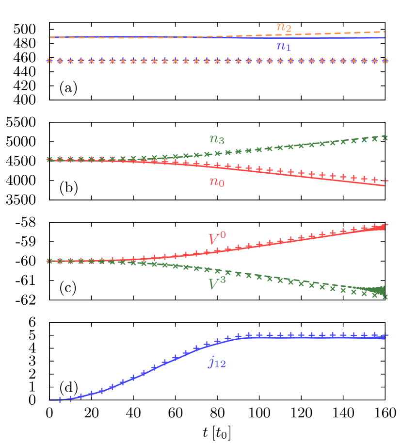
Figure 7: Adiabatic current ramp calculated with variational ansatz (lines) and four-mode model (crosses) for the same system. Shown are (a) particle numbers in the middle wells, (b) particle numbers in outer wells, (c) potential depths of the outer wells in units of $E_{0}$, and (d) particle current $j_{12}$. There are small deviations, but overall the four-mode model is a valid approximation compared to the variational ansatz.

We use the variational ansatz to simulate the adiabatic current ramp of Sec. III.2 (with same parameters) for a BEC in a four-well potential. For simplification, we do not give a specific value of the $\mathcal{PT}$ parameter $\Gamma$ but a target particle current of $j^{\text{tar}}=5/t_{0}$. Fig. 7 shows the results. It is not a priori clear whether the quantity $n_{k}=(d_{\text{eff}}^{k})^{*}d_{\text{eff}}^{k}$ – resulting from the transformed amplitudes of the simplified variational approach – can be compared with the integrated probability density $n_{k}$ of the extended variational approach. We show in App. B that this comparison is indeed possible and reasonable.

Overall, there is the same qualitative behavior between the two approaches. The particle number in the middle wells is slightly under estimated in the four-mode model due to its origin as an approximation. Because of the fixed positions of the outer wells for the variational approach, $n_{1}$ and $n_{2}$ are not exactly equal, but the difference is small compared to the absolute number. We can conclude that we can now also create an (approximate) $\mathcal{PT}$-symmetric state within the variational approach and verify that the results from the four-mode model are a good approximation.

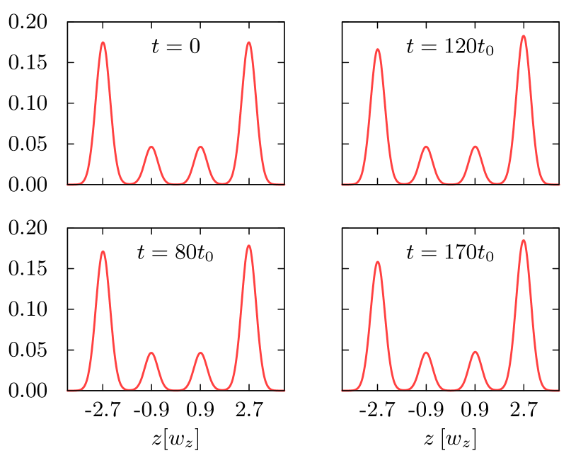
Figure 8: Modulus squared of the wave function $\left|\psi\right|^{2}$ at $x,y=0$ for different times $t$. The amplitudes of the outer parts increase or decrease, whereas the amplitudes in the middle wells stay constant, a clear sign of $\mathcal{PT}$ symmetry, also in an experiment.

The variational approach gives us access to the wave function at each time step (see Fig. 8). As indicated by the particle numbers in Fig. 7, the amplitudes in the middle wells stay almost constant, whereas the amplitudes in the outer wells increase or decrease in time. This could also be measured in an experiment and could serve as a proof of realized $\mathcal{PT}$ symmetry.

V Conclusion

By means of a simple variational ansatz – with localized time-independent Gaussian functions – and the method of symmetric orthogonalization we could transform the GPE for a multi-well potential to a simple few-mode model. The parameters of the variational ansatz are obtained by an energy minimization process in a computationally cheap way. With the results one can, on the one hand, calculate the elements of the few-mode model for a specific system, and on the other determine the parameters of the external potential by knowing the time-dependent matrix elements.

These results are applied to the $\mathcal{PT}$-symmetric two-mode model and to the Hermitian four-mode model. With this model we could show that the four-mode model can be designed in such a way such that the middle wells behave exactly as the two-wells of the $\mathcal{PT}$-symmetric two-mode model. Thus, this Hermitian (closed) system can be used as a possible realization of a quantum mechanical $\mathcal{PT}$-symmetric system. With an extended Gaussian variational ansatz – with full time-dependent Gaussian functions, which can describe a much richer dynamics – we confirmed the qualitative results of the few-mode model.

In this paper we applied the idea to embed a two-well system into a closed system for the simplest case. It is possible for future work to use a greater embedding which could result in a simpler time-dependence of the additional parameters. The ideas presented in this paper could also serve as a possible road map for an investigation of the Bose-Hubbard model and its many-particle effects.

Appendix A Analytical considerations

In Sec. III.1 we derived four conditions [Eqs. (39)] such that the Hermitian four-mode model can simulate the $\mathcal{PT}$-symmetric two-mode model. However, only three of them are independent, which will be shown in this appendix. For that, we need the relations

$$C_{jj}\tilde{j}_{ik} =C_{ij}\tilde{j}_{jk}+\tilde{j}_{ij}C_{jk},$$ (54a)

$$C_{jj}C_{ik} =C_{ij}C_{jk}-\tilde{j}_{ij}\tilde{j}_{jk},$$ (54b)

which can be proved by simply inserting the definitions of these quantities.

We start with Eqs. (39a) and (39b), insert the solutions (40), take the square and use Eqs. (54). We get

$$\tilde{j}_{01}^{2}\tilde{j}_{23}^{2}+\frac{2\Gamma}{d}\tilde{j}_{12}\tilde{j}_{01}\tilde{j}_{23}-C_{12}^{2}\frac{n_{3}}{n_{1}}\tilde{j}_{01}^{2}+\frac{4\Gamma^{2}}{d^{2}}n_{1}n_{2} =0,$$ (55a)

$$\tilde{j}_{01}^{2}\tilde{j}_{23}^{2}+\frac{2\Gamma}{d}\tilde{j}_{12}\tilde{j}_{01}\tilde{j}_{23}-C_{12}^{2}\frac{n_{0}}{n_{2}}\tilde{j}_{23}^{2}+\frac{4\Gamma^{2}}{d^{2}}n_{1}n_{2} =0.$$ (55b)

Taking the difference yields

$$\tilde{j}_{23}^{2} =\frac{n_{2}n_{3}}{n_{0}n_{1}}\tilde{j}_{01}^{2}$$

$$\Leftrightarrow\tilde{j}_{23} =s_{3}\sqrt{\frac{n_{2}n_{3}}{n_{0}n_{1}}}\tilde{j}_{01},$$ (56)

where $s_{3}=\pm 1$ gives the sign of $\tilde{j}_{23}$ compared to $\tilde{j}_{01}$. Inserting this result into Eq. (55a) gives a fourth-order polynomial equation for $\tilde{j}_{01}$. The result is

$$\tilde{j}_{01}=s_{2}\sqrt{2n_{0}n_{1}\left(1-\alpha+s_{1}\sqrt{(1-\alpha)^{2}-\beta^{2}}\right)},$$ (57)

with the definitions

$$\alpha =\frac{\gamma}{2}\left(\beta+\frac{\gamma}{2}\right),$$ (58a)

$$\beta =s_{3}\frac{\Gamma}{d}\frac{1}{\sqrt{n_{0}n_{3}}},$$ (58b)

$$\gamma =\frac{\tilde{j}_{12}}{\sqrt{n_{1}n_{2}}}.$$ (58c)

Using Eqs. (54) we can find all other quantities $\tilde{j}_{kl}$ and $C_{kl}$, especially those needed for the investigation of the fourth condition $J_{01}\tilde{j}_{02}-J_{23}\tilde{j}_{13}=dC_{13}\tilde{j}_{02}-dC_{02}\tilde{j}_{23}$,

$$C_{02} =s_{2}\operatorname{sign}d\sqrt{2n_{0}n_{2}\left(1-\alpha-s_{1}\sqrt{(1-\alpha)^{2}-\beta^{2}}\right)},$$ (59a)

$$C_{13} =s_{2}\operatorname{sign}d\sqrt{2n_{1}n_{3}\left(1-\alpha-s_{1}\sqrt{(1-\alpha)^{2}-\beta^{2}}\right)},$$ (59b)

$$\tilde{j}_{02} =s_{6}\sqrt{2n_{0}n_{2}\left(1+\alpha+s_{1}\sqrt{(1-\alpha)^{2}-\beta^{2}}\right)},$$ (59c)

$$\tilde{j}_{13} =s_{6}\sqrt{2n_{1}n_{3}\left(1+\alpha+s_{1}\sqrt{(1-\alpha)^{2}-\beta^{2}}\right)}.$$ (59d)

All signs $s_{i}$ are determined by the phases of the initial wave function. We can now calculate the fourth condition and find

$$J_{01}\tilde{j}_{02}-J_{23}\tilde{j}_{13}=0.$$ (60)

Thus, the first three conditions of Eqs. (39) imply the validity of the fourth one. With the results of the matrix elements of Sec. III.1, namely $J_{01}$, $J_{23}$, $E_{0}$ and $E_{3}$, we find an exact equivalence of the two- and four-mode models also for interacting atoms. Furthermore, with the results of this appendix, we can calculate these matrix elements, once the quantities $n_{1}$, $n_{2}$ and $\tilde{j}_{12}$ are known.

Appendix B Comparison of probabilities for few-mode-model and Gaussian functions

As discussed in Sec. IV.2 it is not a priori clear whether we can compare the particle numbers obtained from the four-mode model and the extended variational approach. In this appendix we take a closer look at both quantities.

The transformation of the amplitudes from the four-mode model, resulting from symmetric orthogonalization, is given by the inverse of the matrix ${\bm{\mathrm{X}}}$ (cf. Sec. II.3),

$$d_{\text{eff}}^{l} =\sum\limits_{k}({\bm{\mathrm{X}}}^{-1})_{lk}d^{k}$$

$$=\sum\limits_{k}\left[({\bm{\mathrm{X}}}^{-1})^{(0)}_{lk}+({\bm{\mathrm{X}}}^{-1})^{(1)}_{lk}\right]d^{k}.$$ (61)

The individual orders of the inverse matrix can easily be calculated, we get

$$({\bm{\mathrm{X}}}^{-1})_{lk}^{(0)} =\sqrt[4]{\frac{\pi^{3}}{8}}\frac{1}{\sqrt[4]{A_{x,R}^{k}A_{y,R}^{k}A_{z,R}^{k}}}\delta_{lk},$$

$$({\bm{\mathrm{X}}}^{-1})_{lk}^{(1)} =\sqrt[4]{8\pi^{3}}\frac{\sqrt[4]{A_{x,R}^{k}A_{y,R}^{k}A_{z,R}^{k}A_{x,R}^{l}A_{y,R}^{l}A_{z,R}^{l}}}{\sqrt[4]{A_{x,R}^{k}A_{y,R}^{k}A_{z,R}^{k}}+\sqrt[4]{A_{x,R}^{l}A_{y,R}^{l}A_{z,R}^{l}}}$$

$$\quad\times\frac{c^{kl}}{\sqrt{A_{x}^{kl}}\sqrt{A_{y}^{kl}}\sqrt{A_{z}^{kl}}}(\delta_{k,l-1}+\delta_{k,l+1}).$$ (62a)

The main contribution to the particle number $n_{k}=(d_{\text{eff}}^{k})^{*}d_{\text{eff}}^{k}$ is then given by

$$n_{k}=\sqrt{\frac{\pi^{3}}{8}}\frac{1}{\sqrt{A_{x,R}^{k}A_{y,R}^{k}A_{z,R}^{k}}}\left|d^{k}\right|^{2},$$ (63)

plus terms involving neighboring amplitudes.

The extended variational ansatz is given by

$$\psi=\sum\limits_{k}d^{k}\,{\mathrm{e}}^{-A_{x}^{k}x^{2}-A_{y}^{k}y^{2}-A_{z}^{k}(z-q_{z}^{k})^{2}+\mathrm{i}(z-q_{z}^{k})p_{z}^{k}},$$ (64)

with the amplitude $d^{k}=\exp(-\gamma^{k})$. The probability density can then be written as

$$\rho=\sum\limits_{k,l}d^{k}(d^{l})^{*}\,{\mathrm{e}}^{-A_{x}^{kl}x^{2}-A_{y}^{kl}y^{2}-A_{z}^{kl}z^{2}+\mathrm{i}\tilde{p}_{z}^{kl}z-\tilde{\gamma}^{kl}},$$ (65)

with the definitions

$$\tilde{p}_{z}^{kl} =2[A_{z}^{k}q_{z}^{k}+(A_{z}^{l})^{*}q_{z}^{l}]+\mathrm{i}(p_{z}^{k}-p_{z}^{l}),$$ (66a)

$$\tilde{\gamma}^{kl} =A_{z}^{k}(q_{z}^{k})^{2}+(A_{z}^{l})^{*}(q_{z}^{l})^{2}+\mathrm{i}(q_{z}^{k}p_{z}^{k}-q_{z}^{l}p_{z}^{l}).$$ (66b)

We integrate $\rho$ over the region discussed in Sec. IV.1. The integral over $x$ and $y$ yields

$$\rho_{z}=\sum\limits_{k,l}d^{k}(d^{l})^{*}\frac{\pi}{\sqrt{A_{x}^{kl}}\sqrt{A_{y}^{kl}}}\,{\mathrm{e}}^{-A_{z}^{kl}z^{2}+\tilde{p}_{z}^{kl}z-\tilde{\gamma}^{kl}}.$$ (67)

The integral over $z$ goes over a finite interval, say $a\leq z\leq b$, we can express the result in terms of the error function,

$$n(a,b) =\frac{1}{2}\sum\limits_{k,l}d^{k}(d^{l})^{*}\frac{\pi^{3}}{\sqrt{A_{x}^{kl}}\sqrt{A_{y}^{kl}}\sqrt{A_{z}^{kl}}}\,{\mathrm{e}}^{(\tilde{p}_{z}^{kl})^{2}/4A_{z}^{kl}-\tilde{\gamma}^{kl}}$$

$$\times\left[\operatorname{erf}\left(\frac{2A_{z}^{kl}b-\tilde{p}_{z}^{kl}}{4\sqrt{A_{z}^{kl}}}\right)-\operatorname{erf}\left(\frac{2A_{z}^{kl}a-\tilde{p}_{z}^{kl}}{4\sqrt{A_{z}^{kl}}}\right)\right].$$ (68)

To obtain the number of particles in well $i$, we evaluate this expression at points $a$ and $b$ between the wells, we can write $a=q_{z}^{i}-\ell/2$ and $b=q_{z}^{i}+\ell/2$ with $\ell$ the distance between two wells. As in the case for the four-mode model, the main contribution of the sum results for the summand with $i=k=l$. We get approximately

$$n_{i}=\sqrt{\frac{\pi^{3}}{8}}\frac{\operatorname{erf}\left(\sqrt{A_{z,R}^{i}\ell^{2}/2}\right)}{\sqrt{A_{x,R}^{i}A_{y,R}^{i}A_{z,R}^{i}}}\left|d^{i}\right|^{2}.$$ (69)

For typical values of $A_{z,R}^{i}\ell^{2}$ the error function is close to unity. Thus, it is reasonable to compare the particle numbers obtained from the four-mode model [Eq. (63)] with those from the extended variational ansatz [Eq. (69)]. Since the particle currents are given by the derivatives of the particle numbers, this is also the case for the particle currents.