The γγsuperscript𝛾superscript𝛾\gamma^{*}\gamma^{*} total cross section in next-to-leading

order BFKL and LEP2 data


D.Yu. Ivanov, B. Murdaca2† and A. Papa2‡


1 Sobolev Institute of Mathematics and Novosibirsk State University,

630090 Novosibirsk, Russia

2 Dipartimento di Fisica, Università della Calabria,

and Istituto Nazionale di Fisica Nucleare, Gruppo collegato di Cosenza,

Arcavacata di Rende, I-87036 Cosenza, Italy


We study the total cross section for the collision of two highly-virtual photons at large energies, taking into account the BFKL resummation of energy logarithms with full next-to-leading accuracy. A necessary ingredient of the calculation, the next-to-leading order impact factor for the photon to photon transition, has been calculated by Balitsky and Chirilli using an approach based on the operator expansion in Wilson lines. We extracted the result for the photon impact factor in the original BFKL calculation scheme comparing the expression for the photon-photon total cross section obtained in BFKL with the one recently derived by Chirilli and Kovchegov in the Wilson-line operator expansion scheme.

We perform a detailed numerical analysis, combining different, but equivalent in next-to-leading accuracy, representations of the cross section with various optimization methods of the perturbative series. We compare our results with previous determinations in the literature and with the LEP2 experimental data. We find that the account of Balitsky and Chirilli expression for the photon impact factor reduces the BFKL contribution to the cross section to very small values, making it impossible to describe LEP2 data as the sum of BFKL and leading-order QED quark box contributions.

e-mail address:d-ivanov@math.nsc.rue-mail address:beatrice.murdaca@fis.unical.ite-mail address:alessandro.papa@fis.unical.itsuperscripte-mail address:d-ivanov@math.nsc.rusuperscripte-mail address:beatrice.murdaca@fis.unical.itsuperscripte-mail address:alessandro.papa@fis.unical.it\begin{array}[]{ll}{}^{\P}\mbox{{\it e-mail address:}}&\mbox{d-ivanov@math.nsc.ru}\\ {}^{{\dagger}}\mbox{{\it e-mail address:}}&\mbox{beatrice.murdaca@fis.unical.it}\\ {}^{\ddagger}\mbox{{\it e-mail address:}}&\mbox{alessandro.papa@fis.unical.it}\\ \end{array}

1 Introduction

Similarly to the e+esuperscript𝑒superscript𝑒e^{+}e^{-} annihilation into hadrons, the total cross section for the collision of two off-shell photons with large virtualities is an important test ground for perturbative QCD. At a fixed order of αssubscript𝛼𝑠\alpha_{s} and at low energies, the dominant contribution comes from the quark box, calculated at the leading-order (LO) in Refs. [1, 2] (see Fig. 1) and at the next-to-LO (NLO) in Ref. [3]. In Ref. [4] the resummation of double logs appearing in the NLO corrections to the quark box was also studied. At higher energies, the gluon exchange in the t𝑡t-channel overwhelms the quark exchange contribution, due to the different power asymptotics for s𝑠s\to\infty. At higher orders in αssubscript𝛼𝑠\alpha_{s}, the contributions from t𝑡t-channel gluons lead to terms with powers of single logarithms of the energy, which must be resummed.

\begin{picture}(150.0,150.0)(0.0,0.0) \put(0.0,0.0){} \put(0.0,0.0){} \put(0.0,0.0){} \put(0.0,0.0){} \put(0.0,0.0){} \put(0.0,0.0){} \put(0.0,0.0){} \put(0.0,0.0){} \end{picture}
Figure 1: Quark box LO diagrams.

The BFKL approach [5] provides for a consistent theoretical framework for the resummation of the energy logarithms, both in the leading logarithmic approximation (LLA), which means resummation of all terms (αsln(s))nsuperscriptsubscript𝛼𝑠𝑠𝑛(\alpha_{s}\ln(s))^{n}, and in the next-to-leading approximation (NLA), which means resummation of all terms αs(αsln(s))nsubscript𝛼𝑠superscriptsubscript𝛼𝑠𝑠𝑛\alpha_{s}(\alpha_{s}\ln(s))^{n}. In this approach, the imaginary part of the amplitude (and, hence, the total cross section) for a large-s𝑠s hard collision process can be written as the convolution of the Green’s function of two interacting Reggeized gluons with the impact factors of the colliding particles (see Fig. 2).

The study of the γγsuperscript𝛾superscript𝛾\gamma^{*}\gamma^{*} total cross section in LLA BFKL has a long history [6]. For the extension of these results to the NLA level one needs to consider corrections to both the BFKL Green’s function and to the impact factors of colliding virtual photons.

The Green’s function is determined through the BFKL equation and is process-independent. The NLO kernel of the BFKL equation for singlet color representation in the t𝑡t-channel and forward scattering, relevant for the determination of a total cross section in the NLA, has been achieved in Refs. [7], after the long program of calculation of the NLO corrections [8] (for a review, see Ref. [9]).

The other essential ingredient for the γγsuperscript𝛾superscript𝛾\gamma^{*}\gamma^{*} total cross section is the impact factor for the virtual photon to virtual photon transition. While its LO expression is known since long, the NLO calculation, carried out in the momentum representation, turned out to be rather complicated and was completed only after year-long efforts [10]. The lengthy result was published over a few years in pieces, some of them available only in the form of a numerical code, thus making it of limited practical use. Indeed, until very recently, the inclusion of BFKL resummation effects in the NLA calculation of the γγsuperscript𝛾superscript𝛾\gamma^{*}\gamma^{*} total cross section was carried out only in approximate way, by taking the BFKL Green’s function in the NLA while using the LO expression for impact factors. This is the case of the pioneer paper in Ref. [11] (see also Ref. [12]) and of the later analysis in Refs. [13] and [14].

The situation changed radically recently, when the NLO photon impact was calculated in the coordinate space and then transformed to the momentum representation and to the Mellin (or γ𝛾\gamma-representation) [15] (see also Ref. [16]). The NLO expression for the photon impact factor turns out to be very simple in all representations, thus confirming an already well established evidence (see, for instance, Refs. [17]) that the use of the coordinate representation leads to much simpler expressions for the NLO BFKL kernel and impact factors, which, in the momentum representation, would be the result of not so obvious cancellations.

Now all ingredients are available to build the γγsuperscript𝛾superscript𝛾\gamma^{*}\gamma^{*} total cross with full inclusion of the BFKL resummation in the NLA. Indeed, already in Ref. [16] there is a first numerical estimate of the γγsuperscript𝛾superscript𝛾\gamma^{*}\gamma^{*} total cross section in the NLA. Note that, the derivation of the results for the γγsuperscript𝛾superscript𝛾\gamma^{*}\gamma^{*} total cross section in Ref. [16] follows closely the approach developed earlier in Ref. [18], where the high-energy limit of 𝒩=4𝒩4{\cal N}=4 SYM amplitudes was considered. Besides, the authors of Ref. [16] used their formulas for the eigenfunctions of the NLO BFKL kernel derived in Ref. [19].

As a matter of fact, previous studies of physical processes within the BFKL approach in the NLA, such as the photoproduction of two light vector mesons [20, 21, 22] and the production of Mueller-Navelet jets [23, 24], have clearly shown that NLA expressions for an observable (such as a cross-section or an azimuthal correlation), though being formally equivalent up to subleading terms, may lead to somewhat different numerical estimates. At the basis of this observation is the fact that NLO BFKL corrections, both of the kernel and of impact factors, are typically of opposite sign with respect to the LO and large in absolute value. For this reason a numerical estimate cannot be reliable (i) if some optimization procedure for the perturbative series is not applied and (ii) if not corroborated by a careful numerical analysis, aimed at assessing the stability of the result under variation of the original NLA expressions for the observable of interest within a large enough class of NLA-equivalent expressions.

The aim of this paper is to contribute to such analysis, by comparing several NLA-equivalent representations of the γγsuperscript𝛾superscript𝛾\gamma^{*}\gamma^{*} total cross section, in combination with two among the most common methods of optimization of the perturbative series, namely the principle of minimal sensitivity (PMS) [25] and the Brodsky-Lepage-Mackenzie (BLM) method [26]. Moreover, the results of this analysis will be contrasted with the only experimental data available so far, obtained at LEP2 [27, 28].

The paper is organized as follows: In Section 2 we present the general structure of the γγsuperscript𝛾superscript𝛾\gamma^{*}\gamma^{*} total cross section in the NLA and, by comparison with Refs. [15, 16], extract the NLO photon impact factor in the original BFKL calculation scheme; in Section 3 we use this information to build several NLA-equivalent representations of the cross section and present, for each of them, the behavior with the energy in comparison with the LEP2 experimental data; finally, in Section 4, we discuss our results and draw the conclusions.

p1subscript𝑝1p_{1}p1subscript𝑝1p_{1}Φ(q1,s0)Φsubscript𝑞1subscript𝑠0\Phi(\vec{q}_{1},s_{0})q1subscript𝑞1q_{1}q1subscript𝑞1q_{1}q2subscript𝑞2q_{2}q2subscript𝑞2q_{2}G(q1,q2)𝐺subscript𝑞1subscript𝑞2G(\vec{q}_{1},\vec{q}_{2})p2subscript𝑝2p_{2}p2subscript𝑝2p_{2}Φ(q2,s0)Φsubscript𝑞2subscript𝑠0\Phi(-\vec{q}_{2},s_{0})
Figure 2: Schematic representation of the elastic amplitude for the γ(p1)γ(p2)superscript𝛾subscript𝑝1superscript𝛾subscript𝑝2\gamma^{*}(p_{1})\,\gamma^{*}(p_{2}) forward scattering.

2 BFKL contribution to the γγsuperscript𝛾superscript𝛾\gamma^{*}\gamma^{*} total cross section

The total cross section of two unpolarized photons with virtualities Q1subscript𝑄1Q_{1} and Q2subscript𝑄2Q_{2} can be obtained from the imaginary part of the forward amplitude. In LLA BFKL and in the Mellin-representation (also said γ𝛾\gamma- or ν𝜈\nu-representation), it is given by the following expression (see, for instance, Ref. [11]):

σtotγγ(s,Q1,Q2)=i,k=T,L1(2π)2Q1Q2+𝑑ν(Q12Q22)iνFi(ν)Fk(ν)(ss0)α¯sχ(ν),subscriptsuperscript𝜎superscript𝛾superscript𝛾tot𝑠subscript𝑄1subscript𝑄2subscriptformulae-sequence𝑖𝑘𝑇𝐿1superscript2𝜋2subscript𝑄1subscript𝑄2subscriptsuperscriptdifferential-d𝜈superscriptsuperscriptsubscript𝑄12superscriptsubscript𝑄22𝑖𝜈subscript𝐹𝑖𝜈subscript𝐹𝑘𝜈superscript𝑠subscript𝑠0subscript¯𝛼𝑠𝜒𝜈\sigma^{\gamma^{*}\gamma^{*}}_{\rm tot}(s,Q_{1},Q_{2})=\sum_{i,k=T,L}\frac{1}{(2\pi)^{2}Q_{1}Q_{2}}\int\limits^{+\infty}_{-\infty}d\nu\left(\frac{Q_{1}^{2}}{Q_{2}^{2}}\right)^{i\nu}F_{i}(\nu)F_{k}(-\nu)\left(\frac{s}{s_{0}}\right)^{\bar{\alpha}_{s}\chi(\nu)}\;, (1)

where α¯sαs(μR)Nc/πsubscript¯𝛼𝑠subscript𝛼𝑠subscript𝜇𝑅subscript𝑁𝑐𝜋\bar{\alpha}_{s}\equiv\alpha_{s}(\mu_{R})N_{c}/\pi, with Ncsubscript𝑁𝑐N_{c} the number of colors, χ(ν)𝜒𝜈\chi(\nu) is the so-called characteristic BFKL function,

χ(ν)=2ψ(1)ψ(12+iν)ψ(12iν)𝜒𝜈2𝜓1𝜓12𝑖𝜈𝜓12𝑖𝜈\chi(\nu)=2\psi(1)-\psi\left(\frac{1}{2}+i\nu\right)-\psi\left(\frac{1}{2}-i\nu\right) (2)

and

FT(ν)=FT(ν)subscript𝐹𝑇𝜈subscript𝐹𝑇𝜈\displaystyle F_{T}(\nu)=F_{T}(-\nu) =\displaystyle= ααs(qeq2)π2(32iν)(32+iν)Γ2(12iν)Γ2(12+iν)Γ(2iν)Γ(2+iν)𝛼subscript𝛼𝑠subscript𝑞superscriptsubscript𝑒𝑞2𝜋232𝑖𝜈32𝑖𝜈superscriptΓ212𝑖𝜈superscriptΓ212𝑖𝜈Γ2𝑖𝜈Γ2𝑖𝜈\displaystyle\alpha\,\alpha_{s}\left(\sum_{q}e_{q}^{2}\right)\frac{\pi}{2}\frac{(\frac{3}{2}-i\nu)(\frac{3}{2}+i\nu)\Gamma^{2}(\frac{1}{2}-i\nu)\Gamma^{2}(\frac{1}{2}+i\nu)}{\Gamma(2-i\nu)\Gamma(2+i\nu)} (3)
=\displaystyle= ααs(qeq2)π289+4ν2ν(1+ν2)sinh(πν)cosh2(πν),𝛼subscript𝛼𝑠subscript𝑞superscriptsubscript𝑒𝑞2superscript𝜋2894superscript𝜈2𝜈1superscript𝜈2𝜋𝜈superscript2𝜋𝜈\displaystyle\alpha\,\alpha_{s}\left(\sum_{q}e_{q}^{2}\right)\frac{\pi^{2}}{8}\frac{9+4\nu^{2}}{\nu\left(1+\nu^{2}\right)}\frac{\sinh\left(\pi\nu\right)}{\cosh^{2}(\pi\nu)}\,,
FL(ν)=FL(ν)subscript𝐹𝐿𝜈subscript𝐹𝐿𝜈\displaystyle F_{L}(\nu)=F_{L}(-\nu) =\displaystyle= ααs(qeq2)πΓ(32iν)Γ(32+iν)Γ(12iν)Γ(12+iν)Γ(2iν)Γ(2+iν)𝛼subscript𝛼𝑠subscript𝑞superscriptsubscript𝑒𝑞2𝜋Γ32𝑖𝜈Γ32𝑖𝜈Γ12𝑖𝜈Γ12𝑖𝜈Γ2𝑖𝜈Γ2𝑖𝜈\displaystyle\alpha\,\alpha_{s}\left(\sum_{q}e_{q}^{2}\right)\pi\frac{\Gamma(\frac{3}{2}-i\nu)\Gamma(\frac{3}{2}+i\nu)\Gamma(\frac{1}{2}-i\nu)\Gamma(\frac{1}{2}+i\nu)}{\Gamma(2-i\nu)\Gamma(2+i\nu)} (4)
=\displaystyle= ααs(qeq2)π241+4ν2ν(1+ν2)sinh(πν)cosh2(πν)𝛼subscript𝛼𝑠subscript𝑞superscriptsubscript𝑒𝑞2superscript𝜋2414superscript𝜈2𝜈1superscript𝜈2𝜋𝜈superscript2𝜋𝜈\displaystyle\alpha\,\alpha_{s}\left(\sum_{q}e_{q}^{2}\right)\frac{\pi^{2}}{4}\frac{1+4\nu^{2}}{\nu\left(1+\nu^{2}\right)}\frac{\sinh\left(\pi\nu\right)}{\cosh^{2}(\pi\nu)}

are the LO impact factors for transverse and longitudinal polarizations, respectively. In the previous equations, α𝛼\alpha is the electromagnetic coupling constant, the summation extends over all active quarks (taken massless) and eqsubscript𝑒𝑞e_{q} is the quark electric charge in units of the electron charge. In the expression (1) for the LLA BFKL cross section the argument of the strong and electromagnetic coupling constants, μRsubscript𝜇𝑅\mu_{R}, and the value of the scale s0subscript𝑠0s_{0} are not fixed.

Following the procedure of Refs. [21], it is possible to write down the NLA BFKL cross section as follows:

σtotγγ(s,Q1,Q2,s0,μR)=1(2π)2Q1Q2+𝑑ν(Q12Q22)iν(ss0)α¯s(μR)χ(ν)subscriptsuperscript𝜎superscript𝛾superscript𝛾tot𝑠subscript𝑄1subscript𝑄2subscript𝑠0subscript𝜇𝑅1superscript2𝜋2subscript𝑄1subscript𝑄2subscriptsuperscriptdifferential-d𝜈superscriptsuperscriptsubscript𝑄12superscriptsubscript𝑄22𝑖𝜈superscript𝑠subscript𝑠0subscript¯𝛼𝑠subscript𝜇𝑅𝜒𝜈\sigma^{\gamma^{*}\gamma^{*}}_{\rm tot}(s,Q_{1},Q_{2},s_{0},\mu_{R})=\frac{1}{(2\pi)^{2}Q_{1}Q_{2}}\int\limits^{+\infty}_{-\infty}d\nu\left(\frac{Q_{1}^{2}}{Q_{2}^{2}}\right)^{i\nu}\left(\frac{s}{s_{0}}\right)^{\bar{\alpha}_{s}(\mu_{R})\chi(\nu)}
×i,k=T,LFi(ν)Fk(ν){1+α¯s(μR)(Fi(1)(ν,s0,μR)Fi(ν)+Fk(1)(ν,s0,μR)Fk(ν))\times\sum_{i,k=T,L}F_{i}(\nu)F_{k}(-\nu)\left\{1+\bar{\alpha}_{s}(\mu_{R})\left(\frac{F_{i}^{(1)}(\nu,s_{0},\mu_{R})}{F_{i}(\nu)}+\frac{F_{k}^{(1)}(-\nu,s_{0},\mu_{R})}{F_{k}(-\nu)}\right)\right. (5)
+α¯s2(μR)ln(ss0)[χ¯(ν)+β08Ncχ(ν)(χ(ν)+103+2lnμR2Q1Q2)]},\left.+\bar{\alpha}_{s}^{2}(\mu_{R})\ln\left(\frac{s}{s_{0}}\right)\left[\bar{\chi}(\nu)+\frac{\beta_{0}}{8N_{c}}\chi(\nu)\left(-\chi(\nu)+\frac{10}{3}+2\ln\frac{\mu_{R}^{2}}{Q_{1}Q_{2}}\right)\right]\right\}\;,

where

χ¯(ν)¯𝜒𝜈\displaystyle\bar{\chi}(\nu)\, =\displaystyle= 14[π243χ(ν)6ζ(3)χ′′(ν)π3cosh(πν)\displaystyle\,-\frac{1}{4}\left[\frac{\pi^{2}-4}{3}\chi(\nu)-6\zeta(3)-\chi^{\prime\prime}(\nu)-\frac{\pi^{3}}{\cosh(\pi\nu)}\right. (6)
+\displaystyle+ π2sinh(πν)2νcosh2(πν)(3+(1+nfNc3)11+12ν216(1+ν2))+ 4ϕ(ν)],\displaystyle\left.\frac{\pi^{2}\sinh(\pi\nu)}{2\,\nu\,\cosh^{2}(\pi\nu)}\left(3+\left(1+\frac{n_{f}}{N_{c}^{3}}\right)\frac{11+12\nu^{2}}{16(1+\nu^{2})}\right)+\,4\,\phi(\nu)\right]\,,
ϕ(ν)= 201𝑑xcos(νln(x))(1+x)x[π26Li2(x)],Li2(x)=0x𝑑tln(1t)t,formulae-sequenceitalic-ϕ𝜈2superscriptsubscript01differential-d𝑥𝜈𝑥1𝑥𝑥delimited-[]superscript𝜋26subscriptLi2𝑥subscriptLi2𝑥superscriptsubscript0𝑥differential-d𝑡1𝑡𝑡\phi(\nu)\,=\,2\int\limits_{0}^{1}dx\,\frac{\cos(\nu\ln(x))}{(1+x)\sqrt{x}}\left[\frac{\pi^{2}}{6}-\mbox{Li}_{2}(x)\right]\,,\;\;\;\;\;\mbox{Li}_{2}(x)=-\int\limits_{0}^{x}dt\,\frac{\ln(1-t)}{t}\,, (7)

nfsubscript𝑛𝑓n_{f} is the number of active quarks, FL,T(1)(ν,s0,μR)subscriptsuperscript𝐹1𝐿𝑇𝜈subscript𝑠0subscript𝜇𝑅F^{(1)}_{L,T}(\nu,s_{0},\mu_{R}) are the NLO corrections to the longitudinal/transverse photon impact factor in the ν𝜈\nu-representation and

β0=113Nc23nf.subscript𝛽0113subscript𝑁𝑐23subscript𝑛𝑓\beta_{0}=\frac{11}{3}N_{c}-\frac{2}{3}n_{f}\;. (8)

Note that our notations are slightly different in comparison to the ones used in Refs. [21]. The impact factors which we introduced here differ by some factors from the impact factors c1,2subscript𝑐12c_{1,2} (and c1,2(1)subscriptsuperscript𝑐112c^{(1)}_{1,2}) of Refs. [21]:

c1,i(ν)=(Q12)iν1/2Fi(ν)subscript𝑐1𝑖𝜈superscriptsubscriptsuperscript𝑄21𝑖𝜈12subscript𝐹𝑖𝜈\displaystyle c_{1,i}(\nu)=\left(Q^{2}_{1}\right)^{i\nu-1/2}F_{i}(\nu)
c2,k(ν)=(Q22)iν1/2Fk(ν)subscript𝑐2𝑘𝜈superscriptsubscriptsuperscript𝑄22𝑖𝜈12subscript𝐹𝑘𝜈\displaystyle c_{2,k}(\nu)=\left(Q^{2}_{2}\right)^{-i\nu-1/2}F_{k}(-\nu) .absent\displaystyle\,.

Moreover, in the derivation of the last term of Eq. (5) the symmetry property of the LO photon impact factors, FL,T(ν)=FL,T(ν)subscript𝐹𝐿𝑇𝜈subscript𝐹𝐿𝑇𝜈F_{L,T}(\nu)=F_{L,T}(-\nu), was used.

Our goal now is to extract the NLO parts of the photon impact factors, FL,T(1)(ν,s0,μR)subscriptsuperscript𝐹1𝐿𝑇𝜈subscript𝑠0subscript𝜇𝑅F^{(1)}_{L,T}(\nu,s_{0},\mu_{R}), which enter the cross section Eq. (5) in the original BFKL approach, by comparing Eq. (5) with the results for the γγsuperscript𝛾superscript𝛾\gamma^{*}\gamma^{*} cross section obtained recently in the Wilson-line operator expansion scheme by Chirilli and Kovchegov [16]. According to Eqs. (3.40) and (3.41) of Ref. [16], the cross section in the case of transverse and longitudinal polarizations reads

σTT(CK)subscriptsuperscript𝜎CK𝑇𝑇\displaystyle\sigma^{\rm(CK)}_{TT} =\displaystyle= (qeq2)2α2αs2Q1Q2π228+𝑑ν(Q12Q22)iν(sQ1Q2)α¯sχ(ν)+α¯s2χ(1)(ν)superscriptsubscript𝑞superscriptsubscript𝑒𝑞22superscript𝛼2superscriptsubscript𝛼𝑠2subscript𝑄1subscript𝑄2superscript𝜋2superscript28superscriptsubscriptdifferential-d𝜈superscriptsuperscriptsubscript𝑄12superscriptsubscript𝑄22𝑖𝜈superscript𝑠subscript𝑄1subscript𝑄2subscript¯𝛼𝑠𝜒𝜈superscriptsubscript¯𝛼𝑠2superscript𝜒1𝜈\displaystyle\left(\sum_{q}e_{q}^{2}\right)^{2}\frac{\alpha^{2}\alpha_{s}^{2}}{Q_{1}Q_{2}}\frac{\pi^{2}}{2^{8}}\int_{-\infty}^{+\infty}d\nu\left(\frac{Q_{1}^{2}}{Q_{2}^{2}}\right)^{i\nu}\left(\frac{s}{Q_{1}Q_{2}}\right)^{\bar{\alpha}_{s}\chi\left(\nu\right)+\bar{\alpha}_{s}^{2}\chi^{\left(1\right)}\left(\nu\right)} (9)
×\displaystyle\times [(9+4ν2)ν(1+ν2)sinh(πν)cosh2(πν)]2[1+αsπ+α¯s21(ν)][1+αsπ+α¯s21(ν)]superscriptdelimited-[]94superscript𝜈2𝜈1superscript𝜈2𝜋𝜈superscript2𝜋𝜈2delimited-[]1subscript𝛼𝑠𝜋subscript¯𝛼𝑠2subscript1𝜈delimited-[]1subscript𝛼𝑠𝜋subscript¯𝛼𝑠2subscript1𝜈\displaystyle\left[\frac{\left(9+4\nu^{2}\right)}{\nu\left(1+\nu^{2}\right)}\frac{\sinh\left(\pi\nu\right)}{\cosh^{2}(\pi\nu)}\right]^{2}\left[1+\frac{\alpha_{s}}{\pi}+\frac{\bar{\alpha}_{s}}{2}{\cal F}_{1}\left(\nu\right)\right]\left[1+\frac{\alpha_{s}}{\pi}+\frac{\bar{\alpha}_{s}}{2}{\cal F}_{1}\left(-\nu\right)\right]
×\displaystyle\times {1+α¯s[F(ν)]},1subscript¯𝛼𝑠𝐹𝜈\displaystyle\left\{1+\bar{\alpha}_{s}\Re\left[F\left(\nu\right)\right]\right\}\;,
σLL(CK)subscriptsuperscript𝜎CK𝐿𝐿\displaystyle\sigma^{\rm(CK)}_{LL} =\displaystyle= (qeq2)2α2αs2Q1Q2π228+𝑑ν(Q12Q22)iν(sQ1Q2)α¯sχ(ν)+α¯s2χ(1)(ν)superscriptsubscript𝑞superscriptsubscript𝑒𝑞22superscript𝛼2superscriptsubscript𝛼𝑠2subscript𝑄1subscript𝑄2superscript𝜋2superscript28superscriptsubscriptdifferential-d𝜈superscriptsuperscriptsubscript𝑄12superscriptsubscript𝑄22𝑖𝜈superscript𝑠subscript𝑄1subscript𝑄2subscript¯𝛼𝑠𝜒𝜈superscriptsubscript¯𝛼𝑠2superscript𝜒1𝜈\displaystyle\left(\sum_{q}e_{q}^{2}\right)^{2}\frac{\alpha^{2}\alpha_{s}^{2}}{Q_{1}Q_{2}}\frac{\pi^{2}}{2^{8}}\int_{-\infty}^{+\infty}d\nu\left(\frac{Q_{1}^{2}}{Q_{2}^{2}}\right)^{i\nu}\left(\frac{s}{Q_{1}Q_{2}}\right)^{\bar{\alpha}_{s}\chi\left(\nu\right)+\bar{\alpha}_{s}^{2}\chi^{\left(1\right)}\left(\nu\right)} (10)
×\displaystyle\times [(9+4ν2)ν(1+ν2)sinh(πν)cosh2(πν)]2[11+12ν29+4ν2(1+αsπ+α¯s22(ν))\displaystyle\left[\frac{\left(9+4\nu^{2}\right)}{\nu\left(1+\nu^{2}\right)}\frac{\sinh\left(\pi\nu\right)}{\cosh^{2}(\pi\nu)}\right]^{2}\left[\frac{11+12\nu^{2}}{9+4\nu^{2}}\left(1+\frac{\alpha_{s}}{\pi}+\frac{\bar{\alpha}_{s}}{2}{\cal F}_{2}(\nu)\right)\right.
\displaystyle- (1+αsπ+α¯s21(ν))][11+12ν29+4ν2(1+αsπ+α¯s22(ν))\displaystyle\left.\left(1+\frac{\alpha_{s}}{\pi}+\frac{\bar{\alpha}_{s}}{2}{\cal F}_{1}\left(\nu\right)\right)\right]\left[\frac{11+12\nu^{2}}{9+4\nu^{2}}\left(1+\frac{\alpha_{s}}{\pi}+\frac{\bar{\alpha}_{s}}{2}{\cal F}_{2}(-\nu)\right)\right.
\displaystyle- (1+αsπ+α¯s21(ν))]{1+α¯s[F(ν)]},\displaystyle\left.\left(1+\frac{\alpha_{s}}{\pi}+\frac{\bar{\alpha}_{s}}{2}{\cal F}_{1}\left(-\nu\right)\right)\right]\left\{1+\bar{\alpha}_{s}\Re\left[F\left(\nu\right)\right]\right\}\;,

where in the r.h.s. the strong coupling without argument stands for the coupling at the symmetric point, αs=αs(Q1Q2)subscript𝛼𝑠subscript𝛼𝑠subscript𝑄1subscript𝑄2\alpha_{s}=\alpha_{s}(\sqrt{Q_{1}Q_{2}}), [F(ν)]𝐹𝜈\Re\left[F\left(\nu\right)\right] is given in Eq. (3.37) of Ref. [16] and the explicit expressions for 1,2(ν)subscript12𝜈{\cal F}_{1,2}\left(\nu\right) in Eq. (52) of Ref. [15]; for the definition of χ(1)(ν)superscript𝜒1𝜈\chi^{\left(1\right)}\left(\nu\right), see Eqs. (2.9) and (2.11) of Ref. [16], so that

χ(1)(ν)=χ¯(ν)+β08Ncχ(ν)(χ(ν)+103).superscript𝜒1𝜈¯𝜒𝜈subscript𝛽08subscript𝑁𝑐𝜒𝜈𝜒𝜈103\chi^{\left(1\right)}\left(\nu\right)=\bar{\chi}(\nu)+\frac{\beta_{0}}{8N_{c}}\chi(\nu)\left(-\chi(\nu)+\frac{10}{3}\right)\;. (11)

Note that working with NLA accuracy, we replaced in Eqs. (9) and (10) the original factors αs(Q1)αs(Q2)subscript𝛼𝑠subscript𝑄1subscript𝛼𝑠subscript𝑄2\alpha_{s}\left(Q_{1}\right)\alpha_{s}\left(Q_{2}\right) present in Eqs. (3.40) and (3.41) of Ref. [16] by αs2(Q1Q2)superscriptsubscript𝛼𝑠2subscript𝑄1subscript𝑄2\alpha_{s}^{2}(\sqrt{Q_{1}Q_{2}}), since

αs(Q1)αs(Q2)=αs2(Q1Q2)+𝒪(αs4).subscript𝛼𝑠subscript𝑄1subscript𝛼𝑠subscript𝑄2superscriptsubscript𝛼𝑠2subscript𝑄1subscript𝑄2𝒪superscriptsubscript𝛼𝑠4\alpha_{s}\left(Q_{1}\right)\alpha_{s}\left(Q_{2}\right)=\alpha_{s}^{2}(\sqrt{Q_{1}Q_{2}})+{\cal O}(\alpha_{s}^{4})\;.

Another point is that the terms αs/πsubscript𝛼𝑠𝜋\alpha_{s}/\pi which appear in the r.h.s. of Eqs. (9) and (10) are due to the QCD vacuum polarization contribution, which actually reads as 3CFαs/(4π)3subscript𝐶𝐹subscript𝛼𝑠4𝜋3C_{F}\alpha_{s}/(4\pi), where CF=(Nc21)/(2Nc)subscript𝐶𝐹superscriptsubscript𝑁𝑐212subscript𝑁𝑐C_{F}=(N_{c}^{2}-1)/(2N_{c}) 111We are very grateful to the authors of Ref. [16] for the clarification of this issue and for establishing the overall normalization factor in their results for the cross section..

Now we are ready to compare Eqs. (9) and (10) with the BFKL cross section Eq. (5) taken for the particular choice of scales μR2=s0=Q1Q2superscriptsubscript𝜇𝑅2subscript𝑠0subscript𝑄1subscript𝑄2\mu_{R}^{2}=s_{0}=Q_{1}Q_{2}. Expanding Eqs. (9) and (10) into a form similar to Eq. (5) and requiring the coincidence of the two representations for the cross section with NLA accuracy allows us to extract without ambiguity the NLO parts of the BFKL impact factors FL,T(1)(ν,s0,μR)subscriptsuperscript𝐹1𝐿𝑇𝜈subscript𝑠0subscript𝜇𝑅F^{(1)}_{L,T}(\nu,s_{0},\mu_{R}) (at the scale setting s0=μR2=Q1Q2subscript𝑠0superscriptsubscript𝜇𝑅2subscript𝑄1subscript𝑄2s_{0}=\mu_{R}^{2}=Q_{1}Q_{2}):

FT(1)(ν,s0,μR)FT(ν)superscriptsubscript𝐹𝑇1𝜈subscript𝑠0subscript𝜇𝑅subscript𝐹𝑇𝜈\displaystyle\frac{F_{T}^{(1)}(\nu,s_{0},\mu_{R})}{F_{T}(\nu)} =\displaystyle= χ(ν)2lns0Q2+β04NclnμR2Q2𝜒𝜈2subscript𝑠0superscript𝑄2subscript𝛽04subscript𝑁𝑐superscriptsubscript𝜇𝑅2superscript𝑄2\displaystyle\frac{\chi(\nu)}{2}\ln\frac{s_{0}}{Q^{2}}+\frac{\beta_{0}}{4N_{c}}\ln\frac{\mu_{R}^{2}}{Q^{2}}
+\displaystyle+ 3CF4Nc518nfNc+π24+8536π2cosh2(πν)41+4ν2+6χ(ν)9+4ν23subscript𝐶𝐹4subscript𝑁𝑐518subscript𝑛𝑓subscript𝑁𝑐superscript𝜋248536superscript𝜋2superscript2𝜋𝜈414superscript𝜈26𝜒𝜈94superscript𝜈2\displaystyle\frac{3C_{F}}{4N_{c}}-\frac{5}{18}\frac{n_{f}}{N_{c}}+\frac{\pi^{2}}{4}+\frac{85}{36}-\frac{\pi^{2}}{\cosh^{2}(\pi\nu)}-\frac{4}{1+4\nu^{2}}+\frac{6\chi\left(\nu\right)}{9+4\nu^{2}}
+\displaystyle+ 12(12iν)12(1+2iν)718(3+2iν)+203(3+2iν)22518(32iν)1212𝑖𝜈1212𝑖𝜈71832𝑖𝜈203superscript32𝑖𝜈2251832𝑖𝜈\displaystyle\frac{1}{2\left(1-2i\nu\right)}-\frac{1}{2\left(1+2i\nu\right)}-\frac{7}{18\left(3+2i\nu\right)}+\frac{20}{3\left(3+2i\nu\right)^{2}}-\frac{25}{18\left(3-2i\nu\right)}
+\displaystyle+ 12χ(ν)[ψ(12iν)+2ψ(32iν)2ψ(32iν)ψ(52+iν)]12𝜒𝜈delimited-[]𝜓12𝑖𝜈2𝜓32𝑖𝜈2𝜓32𝑖𝜈𝜓52𝑖𝜈\displaystyle\frac{1}{2}\chi\left(\nu\right)\left[\psi\left(\frac{1}{2}-i\nu\right)+2\psi\left(\frac{3}{2}-i\nu\right)-2\psi\left(3-2i\nu\right)-\psi\left(\frac{5}{2}+i\nu\right)\right]

and

FL(1)(ν,s0,μR)FL(ν)superscriptsubscript𝐹𝐿1𝜈subscript𝑠0subscript𝜇𝑅subscript𝐹𝐿𝜈\displaystyle\frac{F_{L}^{(1)}(\nu,s_{0},\mu_{R})}{F_{L}(\nu)} =\displaystyle= χ(ν)2lns0Q2+β04NclnμR2Q2𝜒𝜈2subscript𝑠0superscript𝑄2subscript𝛽04subscript𝑁𝑐superscriptsubscript𝜇𝑅2superscript𝑄2\displaystyle\frac{\chi(\nu)}{2}\ln\frac{s_{0}}{Q^{2}}+\frac{\beta_{0}}{4N_{c}}\ln\frac{\mu_{R}^{2}}{Q^{2}}
+\displaystyle+ 3CF4Nc518nfNc+π24+8536π2cosh2(πν)8(1+4iν)(1+2iν)2(12iν)(3+2iν)3subscript𝐶𝐹4subscript𝑁𝑐518subscript𝑛𝑓subscript𝑁𝑐superscript𝜋248536superscript𝜋2superscript2𝜋𝜈814𝑖𝜈superscript12𝑖𝜈212𝑖𝜈32𝑖𝜈\displaystyle\frac{3C_{F}}{4N_{c}}-\frac{5}{18}\frac{n_{f}}{N_{c}}+\frac{\pi^{2}}{4}+\frac{85}{36}-\frac{\pi^{2}}{\cosh^{2}(\pi\nu)}-\frac{8\left(1+4i\nu\right)}{\left(1+2i\nu\right)^{2}\left(1-2i\nu\right)\left(3+2i\nu\right)}
+\displaystyle+ 434iν+4ν2χ(ν)434𝑖𝜈4superscript𝜈2𝜒𝜈\displaystyle\frac{4}{3-4i\nu+4\nu^{2}}\chi\left(\nu\right)
+\displaystyle+ 12χ(ν)[ψ(12iν)+2ψ(32iν)2ψ(32iν)ψ(52+iν)].12𝜒𝜈delimited-[]𝜓12𝑖𝜈2𝜓32𝑖𝜈2𝜓32𝑖𝜈𝜓52𝑖𝜈\displaystyle\frac{1}{2}\chi\left(\nu\right)\left[\psi\left(\frac{1}{2}-i\nu\right)+2\psi\left(\frac{3}{2}-i\nu\right)-2\psi\left(3-2i\nu\right)-\psi\left(\frac{5}{2}+i\nu\right)\right]\;.

The first lines of Eqs. (2) and (2) describe the dependencies of the photon impact factors on the renormalization and energy scales, which are restored by the requirement that the BFKL cross section, Eq. (5), does not depend on s0subscript𝑠0s_{0} and μRsubscript𝜇𝑅\mu_{R} with NLA accuracy.

3 Numerical analysis

In this Section we are going to compare several different representations of the NLA γγsuperscript𝛾superscript𝛾\gamma^{*}\gamma^{*} total cross section, which differ one from the other only by terms beyond the NLA. In a well-behaved perturbative series, the change of representation should not be numerically relevant. This is not the case in the BFKL framework, where it is well known that NLO corrections to kernel and impact factors are opposite in sign with respect to the LO contributions and large in absolute value.

It is very likely that also the (unknown) next-to-NLO corrections maybe opposite in sign with respect the NLO ones and large in absolute value, thus suggesting that fixing the BFKL energy scale s0subscript𝑠0s_{0} and the renormalization scale μRsubscript𝜇𝑅\mu_{R} at the “natural” values dictated by the kinematics of the process, i.e. s0=μR2=Q1Q2subscript𝑠0superscriptsubscript𝜇𝑅2subscript𝑄1subscript𝑄2s_{0}=\mu_{R}^{2}=Q_{1}Q_{2}, may well be not the best choice. For this reason, we will consider in the following two alternative procedures to fix the energy scales.

The first one is inspired by the PMS optimization method [25]: for each value of the center-of-mass energy s𝑠s and of the virtualities of the colliding photons, we choose as optimal scales s0subscript𝑠0s_{0} and μRsubscript𝜇𝑅\mu_{R} those for which the given representation of the NLA cross section exhibits the minimum sensitivity under variation of these scales.

The other optimization procedure we consider is inspired by the BLM method [26]: again, for fixed s𝑠s and photon virtualities, we perform a finite renormalization to a momentum (MOM) scheme and then choose the renormalization scale μRsubscript𝜇𝑅\mu_{R} in order to remove the β0subscript𝛽0\beta_{0}-dependent part in the given representation of the NLA cross section, while keeping the scale s0subscript𝑠0s_{0} fixed at the natural value Q1Q2subscript𝑄1subscript𝑄2Q_{1}Q_{2}. In fact, there is some freedom in implementing the BLM optimization in this context and in the following we consider two different variants, dubbed (a)𝑎(a) and (b)𝑏(b), and give all necessary formulas, but relegate their derivation to a separate paper [29].

Below we will present predictions for the kinematic range relevant for the OPAL and L3 experiments at LEP2, considering equal photon virtualities, Q1=Q2Qsubscript𝑄1subscript𝑄2𝑄Q_{1}=Q_{2}\equiv Q, with Q2superscript𝑄2Q^{2}=17 GeV2, and the energy range Y=2÷6𝑌26Y=2\div 6, where Yln(s/Q2)𝑌𝑠superscript𝑄2Y\equiv\ln(s/Q^{2}).

3.1 Chirilli-Kovchegov representation

As a first case, we try to apply to the description of LEP2 data the representation of the NLA γγsuperscript𝛾superscript𝛾\gamma^{*}\gamma^{*} total cross section given in Ref. [16]. It is given, with obvious meaning of the notation, by

σtot(CK)(s,Q)=σTT(CK)+σLL(CK)+σTL(CK)+σLT(CK)+σLObox,subscriptsuperscript𝜎CKtot𝑠𝑄subscriptsuperscript𝜎CK𝑇𝑇subscriptsuperscript𝜎CK𝐿𝐿subscriptsuperscript𝜎CK𝑇𝐿subscriptsuperscript𝜎CK𝐿𝑇subscript𝜎LObox\sigma^{\rm(CK)}_{\rm tot}(s,Q)=\sigma^{\rm(CK)}_{TT}+\sigma^{\rm(CK)}_{LL}+\sigma^{\rm(CK)}_{TL}+\sigma^{\rm(CK)}_{LT}+\sigma_{\rm LO\ box}\;, (14)

where we have included the LO contribution from the quark box, given in Refs. [1, 2], and contributions of different polarization states of virtual photons. The explicit expressions for the first two terms in Eq. (14) are given in Eqs. (9) and (10) (for Q1=Q2=Qsubscript𝑄1subscript𝑄2𝑄Q_{1}=Q_{2}=Q), the contributions of other polarizations can be obviously presented as follows:

σTL(CK)subscriptsuperscript𝜎CK𝑇𝐿\displaystyle\sigma^{\rm(CK)}_{TL} =\displaystyle= (qeq2)2α2αs2Q2π228+𝑑ν(sQ2)α¯sχ(ν)+α¯s2χ(1)(ν)superscriptsubscript𝑞superscriptsubscript𝑒𝑞22superscript𝛼2superscriptsubscript𝛼𝑠2superscript𝑄2superscript𝜋2superscript28superscriptsubscriptdifferential-d𝜈superscript𝑠superscript𝑄2subscript¯𝛼𝑠𝜒𝜈superscriptsubscript¯𝛼𝑠2superscript𝜒1𝜈\displaystyle\left(\sum_{q}e_{q}^{2}\right)^{2}\frac{\alpha^{2}\alpha_{s}^{2}}{Q^{2}}\frac{\pi^{2}}{2^{8}}\int_{-\infty}^{+\infty}d\nu\left(\frac{s}{Q^{2}}\right)^{\bar{\alpha}_{s}\chi\left(\nu\right)+\bar{\alpha}_{s}^{2}\chi^{\left(1\right)}\left(\nu\right)} (15)
×\displaystyle\times [(9+4ν2)ν(1+ν2)sinh(πν)cosh2(πν)]2[1+αsπ+α¯s21(ν)]superscriptdelimited-[]94superscript𝜈2𝜈1superscript𝜈2𝜋𝜈superscript2𝜋𝜈2delimited-[]1subscript𝛼𝑠𝜋subscript¯𝛼𝑠2subscript1𝜈\displaystyle\left[\frac{\left(9+4\nu^{2}\right)}{\nu\left(1+\nu^{2}\right)}\frac{\sinh\left(\pi\nu\right)}{\cosh^{2}(\pi\nu)}\right]^{2}\left[1+\frac{\alpha_{s}}{\pi}+\frac{\bar{\alpha}_{s}}{2}{\cal F}_{1}\left(\nu\right)\right]
×\displaystyle\times [11+12ν29+4ν2(1+αsπ+α¯s22(ν))\displaystyle\left[\frac{11+12\nu^{2}}{9+4\nu^{2}}\left(1+\frac{\alpha_{s}}{\pi}+\frac{\bar{\alpha}_{s}}{2}{\cal F}_{2}(-\nu)\right)\right.
\displaystyle- (1+αsπ+α¯s21(ν))]{1+α¯s[F(ν)]},\displaystyle\left.\left(1+\frac{\alpha_{s}}{\pi}+\frac{\bar{\alpha}_{s}}{2}{\cal F}_{1}\left(-\nu\right)\right)\right]\left\{1+\bar{\alpha}_{s}\Re\left[F\left(\nu\right)\right]\right\}\;,
σLT(CK)subscriptsuperscript𝜎CK𝐿𝑇\displaystyle\sigma^{\rm(CK)}_{LT} =\displaystyle= (qeq2)2α2αs2Q2π228+𝑑ν(sQ2)α¯sχ(ν)+α¯s2χ(1)(ν)superscriptsubscript𝑞superscriptsubscript𝑒𝑞22superscript𝛼2superscriptsubscript𝛼𝑠2superscript𝑄2superscript𝜋2superscript28superscriptsubscriptdifferential-d𝜈superscript𝑠superscript𝑄2subscript¯𝛼𝑠𝜒𝜈superscriptsubscript¯𝛼𝑠2superscript𝜒1𝜈\displaystyle\left(\sum_{q}e_{q}^{2}\right)^{2}\frac{\alpha^{2}\alpha_{s}^{2}}{Q^{2}}\frac{\pi^{2}}{2^{8}}\int_{-\infty}^{+\infty}d\nu\left(\frac{s}{Q^{2}}\right)^{\bar{\alpha}_{s}\chi\left(\nu\right)+\bar{\alpha}_{s}^{2}\chi^{\left(1\right)}\left(\nu\right)} (16)
×\displaystyle\times [(9+4ν2)ν(1+ν2)sinh(πν)cosh2(πν)]2[1+αsπ+α¯s21(ν)]superscriptdelimited-[]94superscript𝜈2𝜈1superscript𝜈2𝜋𝜈superscript2𝜋𝜈2delimited-[]1subscript𝛼𝑠𝜋subscript¯𝛼𝑠2subscript1𝜈\displaystyle\left[\frac{\left(9+4\nu^{2}\right)}{\nu\left(1+\nu^{2}\right)}\frac{\sinh\left(\pi\nu\right)}{\cosh^{2}(\pi\nu)}\right]^{2}\left[1+\frac{\alpha_{s}}{\pi}+\frac{\bar{\alpha}_{s}}{2}{\cal F}_{1}\left(-\nu\right)\right]
×\displaystyle\times [11+12ν29+4ν2(1+αsπ+α¯s22(ν))\displaystyle\left[\frac{11+12\nu^{2}}{9+4\nu^{2}}\left(1+\frac{\alpha_{s}}{\pi}+\frac{\bar{\alpha}_{s}}{2}{\cal F}_{2}(\nu)\right)\right.
\displaystyle- (1+αsπ+α¯s21(ν))]{1+α¯s[F(ν)]},\displaystyle\left.\left(1+\frac{\alpha_{s}}{\pi}+\frac{\bar{\alpha}_{s}}{2}{\cal F}_{1}\left(\nu\right)\right)\right]\left\{1+\bar{\alpha}_{s}\Re\left[F\left(\nu\right)\right]\right\}\;,

where αs=αs(Q)subscript𝛼𝑠subscript𝛼𝑠𝑄\alpha_{s}=\alpha_{s}(Q), 1,2(ν)subscript12𝜈{\cal F}_{1,2}(\nu) and [F(ν)]𝐹𝜈\Re[F(\nu)] are given in Eq. (52) of [15] and in Eq. (3.37) of [16], respectively.

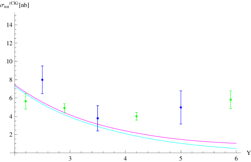
In Fig. 3 we report the behavior of σtot(CK)subscriptsuperscript𝜎CKtot\sigma^{\rm(CK)}_{\rm tot} with Yln(s/Q2)𝑌𝑠superscript𝑄2Y\equiv\ln(s/Q^{2}) for Q2superscript𝑄2Q^{2}=17 GeV2 with nf=4subscript𝑛𝑓4n_{f}=4 and contrast it with the experimental data from CERN LEP2, namely three data points from OPAL [28] (Q2superscript𝑄2Q^{2}=18 GeV2) and four data points from L3 [27] (Q2superscript𝑄2Q^{2}=16 GeV2). We see that the original Chirilli-Kovchegov representation for the cross section (at natural values of the scales, s0=μR2=Q2subscript𝑠0superscriptsubscript𝜇𝑅2superscript𝑄2s_{0}=\mu_{R}^{2}=Q^{2}) gives a very small BFKL contribution and does not agree well with data above Y=4𝑌4Y=4.

Refer to caption
Figure 3: σtot(CK)subscriptsuperscript𝜎CKtot\sigma^{\rm(CK)}_{\rm tot} versus Y𝑌Y at Q2=17superscript𝑄217Q^{2}=17 GeV2 (nf=4subscript𝑛𝑓4n_{f}=4) (magenta line), together with the experimental data from OPAL (blue points, Q2=18superscript𝑄218Q^{2}=18 GeV2) and L3 (green points, Q2=16superscript𝑄216Q^{2}=16 GeV2); the cyan line represents the LO quark box contribution only.

In the following subsections, we are going to consider other representations of the cross section, equivalent to the Chirilli-Kovchegov one within the NLA, and admit the possibility of moving the energy scale s0subscript𝑠0s_{0} and the renormalization scale μFsubscript𝜇𝐹\mu_{F} from the “natural” kinematic value to some “optimal” scales, determined according the PMS or the BLM methods.

3.2 Series representation with PMS optimization

A convenient representation of the total cross section is the so-called “series representation”, already used in Refs. [21, 22], which has the advantage of making manifest the BFKL resummation of leading and subleading energy logarithms and is very practical in numerical computations. It consists in writing the total cross section as follows

σtot(series)(s,Q)=σTT(series)+σLL(series)+σTL(series)+σLT(series)+σLObox,subscriptsuperscript𝜎seriestot𝑠𝑄subscriptsuperscript𝜎series𝑇𝑇subscriptsuperscript𝜎series𝐿𝐿subscriptsuperscript𝜎series𝑇𝐿subscriptsuperscript𝜎series𝐿𝑇subscript𝜎LObox\sigma^{\rm(series)}_{\rm tot}(s,Q)=\sigma^{\rm(series)}_{TT}+\sigma^{\rm(series)}_{LL}+\sigma^{\rm(series)}_{TL}+\sigma^{\rm(series)}_{LT}+\sigma_{\rm LO\ box}\;, (17)

where for i,k=L,Tformulae-sequence𝑖𝑘𝐿𝑇i,k=L,T

Q2σik(series)superscript𝑄2subscriptsuperscript𝜎series𝑖𝑘\displaystyle Q^{2}\sigma^{\rm(series)}_{ik} =\displaystyle= 1(2π)2{b0ik+n=1α¯sn(μR)bnik[(YY0)n+dnik(s0,μR)(YY0)n1]},1superscript2𝜋2superscriptsubscript𝑏0𝑖𝑘superscriptsubscript𝑛1superscriptsubscript¯𝛼𝑠𝑛subscript𝜇𝑅superscriptsubscript𝑏𝑛𝑖𝑘delimited-[]superscript𝑌subscript𝑌0𝑛superscriptsubscript𝑑𝑛𝑖𝑘subscript𝑠0subscript𝜇𝑅superscript𝑌subscript𝑌0𝑛1\displaystyle\frac{1}{\left(2\pi\right)^{2}}\left\{b_{0}^{ik}+\sum_{n=1}^{\infty}\bar{\alpha}_{s}^{n}(\mu_{R})\ b_{n}^{ik}\left[\left(Y-Y_{0}\right)^{n}+d_{n}^{ik}(s_{0},\mu_{R})\left(Y-Y_{0}\right)^{n-1}\right]\right\}\;, (18)

with Y0ln(s0/Q2)subscript𝑌0subscript𝑠0superscript𝑄2Y_{0}\equiv\ln(s_{0}/Q^{2}) and

bnik=+𝑑νFi(ν)Fk(ν)χn(ν)n!,superscriptsubscript𝑏𝑛𝑖𝑘superscriptsubscriptdifferential-d𝜈subscript𝐹𝑖𝜈subscript𝐹𝑘𝜈superscript𝜒𝑛𝜈𝑛b_{n}^{ik}=\int_{-\infty}^{+\infty}d\nu F_{i}\left(\nu\right)F_{k}\left(-\nu\right)\frac{\chi^{n}\left(\nu\right)}{n!}\;, (19)
dniksuperscriptsubscript𝑑𝑛𝑖𝑘\displaystyle d_{n}^{ik} =\displaystyle= nlns0Q2+β04Nc[bn1ikbnik((n+1)lnμR2Q2+53(n1))n(n1)2]𝑛subscript𝑠0superscript𝑄2subscript𝛽04subscript𝑁𝑐delimited-[]superscriptsubscript𝑏𝑛1𝑖𝑘superscriptsubscript𝑏𝑛𝑖𝑘𝑛1superscriptsubscript𝜇𝑅2superscript𝑄253𝑛1𝑛𝑛12\displaystyle n\ln\frac{s_{0}}{Q^{2}}+\frac{\beta_{0}}{4N_{c}}\left[\frac{b_{n-1}^{ik}}{b_{n}^{ik}}\left(\left(n+1\right)\ln\frac{\mu_{R}^{2}}{Q^{2}}+\frac{5}{3}\left(n-1\right)\right)-\frac{n\left(n-1\right)}{2}\right]
+\displaystyle+ 1bnik+𝑑νFi(ν)Fk(ν)[χn1(ν)(n1)!(F¯i(1)(ν)Fi(ν)+F¯k(1)(ν)Fk(ν))+χn2(ν)(n2)!χ¯(ν)],1superscriptsubscript𝑏𝑛𝑖𝑘superscriptsubscriptdifferential-d𝜈subscript𝐹𝑖𝜈subscript𝐹𝑘𝜈delimited-[]superscript𝜒𝑛1𝜈𝑛1superscriptsubscript¯𝐹𝑖1𝜈subscript𝐹𝑖𝜈superscriptsubscript¯𝐹𝑘1𝜈subscript𝐹𝑘𝜈superscript𝜒𝑛2𝜈𝑛2¯𝜒𝜈\displaystyle\frac{1}{b_{n}^{ik}}\int_{-\infty}^{+\infty}d\nu\,F_{i}\left(\nu\right)F_{k}\left(-\nu\right)\left[\frac{\chi^{n-1}\left(\nu\right)}{\left(n-1\right)!}\left(\frac{\bar{F}_{i}^{(1)}(\nu)}{F_{i}(\nu)}+\frac{\bar{F}_{k}^{(1)}(-\nu)}{F_{k}(-\nu)}\right)+\frac{\chi^{n-2}\left(\nu\right)}{\left(n-2\right)!}\bar{\chi}\left(\nu\right)\right]\;,

where we denoted for shortness F¯i(1)(ν)Fi(1)(ν,s0=Q2,μR=Q)\bar{F}_{i}^{(1)}(\nu)\equiv F_{i}^{(1)}\left(\nu,s_{0}=Q^{2},\mu_{R}=Q\right).

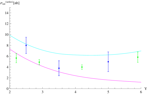
Our results for σtot(series)subscriptsuperscript𝜎seriestot\sigma^{\rm(series)}_{\rm tot} at Q2superscript𝑄2Q^{2}=17 GeV2, obtained after truncation of the series at n=40𝑛40n=40, are summarized in Table 1, where we report, for each of the Y𝑌Y values considered, also the optimal values of the energy scale Y0subscript𝑌0Y_{0} and renormalization scale μRsubscript𝜇𝑅\mu_{R} found by the PMS method. In Fig. 4 we compare an interpolation of the data given in Table 1 with the experimental data from LEP2 and with the result obtained in Ref. [13] by the same method, but in the approximation where LO photon impact factors were used instead of NLO ones (i.e. the same approach as here, but with F¯i(1)(ν)0superscriptsubscript¯𝐹𝑖1𝜈0\bar{F}_{i}^{(1)}(\nu)\to 0). We observe that the large optimal values for the scales we find in this approach lead to a very low contribution to the cross section from the BFKL resummation and the overall scenario is basically the same as for the Chirilli-Kovchegov representation. We note that the big difference between this and the approximated result obtained in Ref. [13] is a clear indication that the effect of NLO corrections to the impact factors is very substantial.

Table 1: Values of σtot(series)subscriptsuperscript𝜎seriestot\sigma^{\rm(series)}_{\rm tot} for several values of Y𝑌Y at Q2=17superscript𝑄217Q^{2}=17 GeV2; the last two columns give the optimal values of the renormalization and energy scales.
Y𝑌Y σtot(series)subscriptsuperscript𝜎seriestot\sigma^{\rm(series)}_{\rm tot}[nb] μR/Qsubscript𝜇𝑅𝑄\mu_{R}/Q Y0subscript𝑌0Y_{0}
2 7.3141 18 1
3.5 3.1095 10 3
4.5 1.9187 10 4
6 1.1909 16 5
Refer to caption
Figure 4: σtot(series)subscriptsuperscript𝜎seriestot\sigma^{\rm(series)}_{\rm tot} versus Y𝑌Y at Q2=17superscript𝑄217Q^{2}=17 GeV2 (nf=4subscript𝑛𝑓4n_{f}=4) (magenta line), together with the experimental data from OPAL (blue points, Q2=18superscript𝑄218Q^{2}=18 GeV2) and L3 (green points, Q2=16superscript𝑄216Q^{2}=16 GeV2); the cyan line represents the result of Ref. [13] (see Fig. 3 there).

3.3 Exponential representation with PMS optimization

Here we consider representations of the NLA total cross section where the NLO corrections to the kernel are exponentiated, in two options, which differ by a subleading term given by the product of the two NLO corrections of the photon impact factors:

σtot(exp, 1)(s,Q)=σTT(exp, 1)+σLL(exp, 1)+σTL(exp, 1)+σLT(exp, 1)+σLObox,subscriptsuperscript𝜎exp1tot𝑠𝑄subscriptsuperscript𝜎exp1𝑇𝑇subscriptsuperscript𝜎exp1𝐿𝐿subscriptsuperscript𝜎exp1𝑇𝐿subscriptsuperscript𝜎exp1𝐿𝑇subscript𝜎LObox\sigma^{\rm(exp,\ 1)}_{\rm tot}(s,Q)=\sigma^{\rm(exp,\ 1)}_{TT}+\sigma^{\rm(exp,\ 1)}_{LL}+\sigma^{\rm(exp,\ 1)}_{TL}+\sigma^{\rm(exp,\ 1)}_{LT}+\sigma_{\rm LO\ box}\;, (21)

and

σtot(exp, 2)(s,Q)=σTT(exp, 2)+σLL(exp, 2)+σTL(exp, 2)+σLT(exp, 2)+σLObox,subscriptsuperscript𝜎exp2tot𝑠𝑄subscriptsuperscript𝜎exp2𝑇𝑇subscriptsuperscript𝜎exp2𝐿𝐿subscriptsuperscript𝜎exp2𝑇𝐿subscriptsuperscript𝜎exp2𝐿𝑇subscript𝜎LObox\sigma^{\rm(exp,\ 2)}_{\rm tot}(s,Q)=\sigma^{\rm(exp,\ 2)}_{TT}+\sigma^{\rm(exp,\ 2)}_{LL}+\sigma^{\rm(exp,\ 2)}_{TL}+\sigma^{\rm(exp,\ 2)}_{LT}+\sigma_{\rm LO\ box}\;, (22)

with

σik(exp, 1)subscriptsuperscript𝜎exp1𝑖𝑘\displaystyle\sigma^{\rm(exp,\ 1)}_{ik} =\displaystyle= 1(2π)2Q2+𝑑νe(YY0)[α¯s(μR)(1+α¯s(μR)β04NclnμR2Q2)χ(ν)+α¯s2(μR)χ(1)(ν)]1superscript2𝜋2superscript𝑄2superscriptsubscriptdifferential-d𝜈superscript𝑒𝑌subscript𝑌0delimited-[]subscript¯𝛼𝑠subscript𝜇𝑅1subscript¯𝛼𝑠subscript𝜇𝑅subscript𝛽04subscript𝑁𝑐superscriptsubscript𝜇𝑅2superscript𝑄2𝜒𝜈superscriptsubscript¯𝛼𝑠2subscript𝜇𝑅superscript𝜒1𝜈\displaystyle\frac{1}{\left(2\pi\right)^{2}Q^{2}}\int_{-\infty}^{+\infty}d\nu\ e^{\left(Y-Y_{0}\right)\left[\bar{\alpha}_{s}\left(\mu_{R}\right)\left(1+\frac{\bar{\alpha}_{s}\left(\mu_{R}\right)\beta_{0}}{4N_{c}}\ln\frac{\mu_{R}^{2}}{Q^{2}}\right)\chi\left(\nu\right)+\bar{\alpha}_{s}^{2}\left(\mu_{R}\right)\chi^{\left(1\right)}\left(\nu\right)\right]} (23)
×\displaystyle\times Fi(ν)Fk(ν)[1+α¯s(μR)(Fi(1)(ν)Fi(ν)+Fk(1)(ν)Fk(ν))]subscript𝐹𝑖𝜈subscript𝐹𝑘𝜈delimited-[]1subscript¯𝛼𝑠subscript𝜇𝑅superscriptsubscript𝐹𝑖1𝜈subscript𝐹𝑖𝜈superscriptsubscript𝐹𝑘1𝜈subscript𝐹𝑘𝜈\displaystyle F_{i}(\nu)F_{k}(-\nu)\left[1+\bar{\alpha}_{s}\left(\mu_{R}\right)\left(\frac{F_{i}^{(1)}(\nu)}{F_{i}(\nu)}+\frac{F_{k}^{(1)}(-\nu)}{F_{k}(-\nu)}\right)\right]

and

σik(exp, 2)subscriptsuperscript𝜎exp2𝑖𝑘\displaystyle\sigma^{\rm(exp,\ 2)}_{ik} =\displaystyle= 1(2π)2Q2+𝑑νe(YY0)[α¯s(μR)(1+α¯s(μR)β04NclnμR2Q2)χ(ν)+α¯s2(μR)χ(1)(ν)]1superscript2𝜋2superscript𝑄2superscriptsubscriptdifferential-d𝜈superscript𝑒𝑌subscript𝑌0delimited-[]subscript¯𝛼𝑠subscript𝜇𝑅1subscript¯𝛼𝑠subscript𝜇𝑅subscript𝛽04subscript𝑁𝑐superscriptsubscript𝜇𝑅2superscript𝑄2𝜒𝜈superscriptsubscript¯𝛼𝑠2subscript𝜇𝑅superscript𝜒1𝜈\displaystyle\frac{1}{\left(2\pi\right)^{2}Q^{2}}\int_{-\infty}^{+\infty}d\nu\ e^{\left(Y-Y_{0}\right)\left[\bar{\alpha}_{s}\left(\mu_{R}\right)\left(1+\frac{\bar{\alpha}_{s}\left(\mu_{R}\right)\beta_{0}}{4N_{c}}\ln\frac{\mu_{R}^{2}}{Q^{2}}\right)\chi\left(\nu\right)+\bar{\alpha}_{s}^{2}\left(\mu_{R}\right)\chi^{\left(1\right)}\left(\nu\right)\right]} (24)
×\displaystyle\times Fi(ν)Fk(ν)[1+α¯s(μR)(Fi(1)(ν)Fi(ν)+Fk(1)(ν)Fk(ν))\displaystyle F_{i}(\nu)F_{k}(-\nu)\left[1+\bar{\alpha}_{s}\left(\mu_{R}\right)\left(\frac{F_{i}^{(1)}(\nu)}{F_{i}(\nu)}+\frac{F_{k}^{(1)}(-\nu)}{F_{k}(-\nu)}\right)\right.
+\displaystyle+ α¯s2(μR)(Fi(1)(ν)Fi(ν)Fk(1)(ν)Fk(ν))].\displaystyle\left.\bar{\alpha}_{s}^{2}\left(\mu_{R}\right)\left(\frac{F_{i}^{(1)}(\nu)}{F_{i}(\nu)}\frac{F_{k}^{(1)}(-\nu)}{F_{k}(-\nu)}\right)\right]\,.

In these equations we denote for shortness Fi,k(1)(ν)Fi,k(1)(ν,s0,μR)superscriptsubscript𝐹𝑖𝑘1𝜈superscriptsubscript𝐹𝑖𝑘1𝜈subscript𝑠0subscript𝜇𝑅F_{i,k}^{(1)}(\nu)\equiv F_{i,k}^{(1)}(\nu,s_{0},\mu_{R}).

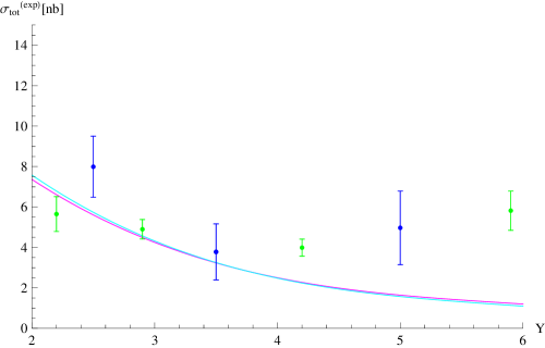
We used these two exponentiated representations together with the PMS method to fix the values of the energy scales and obtained the results given in Table 2. We can see that the variant (2) of the exponentiated cross section gets lower values for the optimal energy scales, thus implying that the inclusion of the subleading term with the product of the NLO impact factors catches a relevant part of the unknown next-to-NLA corrections. However, as shown in Fig. 5, the absolute value of the cross section remains low and undershoots LEP2 data substantially in the same fashion as the two previous representations.

Table 2: Values of σtot(exp, 1,2)subscriptsuperscript𝜎exp12tot\sigma^{\rm(exp,\ 1,2)}_{\rm tot} for several values of Y𝑌Y at Q2=17superscript𝑄217Q^{2}=17 GeV2; the columns 3-4 and 6-7 give the optimal values of the renormalization and energy scales.
Y𝑌Y σtot(exp, 1)subscriptsuperscript𝜎exp1tot\sigma^{\rm(exp,\ 1)}_{\rm tot}[nb] μR/Qsubscript𝜇𝑅𝑄\mu_{R}/Q Y0subscript𝑌0Y_{0} σtot(exp, 2)subscriptsuperscript𝜎exp2tot\sigma^{\rm(exp,\ 2)}_{\rm tot}[nb] μR/Qsubscript𝜇𝑅𝑄\mu_{R}/Q Y0subscript𝑌0Y_{0}
2 7.36281 18 1 7.57706 8 1
3.5 3.23512 18 3 3.25243 8 1
4.5 1.98923 18 4 1.9419 8 1
6 1.20222 18 5 1.09588 8 1
Refer to caption
Figure 5: σtot(exp, 1)subscriptsuperscript𝜎exp1tot\sigma^{\rm(exp,\ 1)}_{\rm tot} (magenta line) and σtot(exp, 2)subscriptsuperscript𝜎exp2tot\sigma^{\rm(exp,\ 2)}_{\rm tot} (cyan line) versus Y𝑌Y at Q2=17superscript𝑄217Q^{2}=17 GeV2 (nf=4subscript𝑛𝑓4n_{f}=4), together with the experimental data from OPAL (blue points, Q2=18superscript𝑄218Q^{2}=18 GeV2) and L3 (green points, Q2=16superscript𝑄216Q^{2}=16 GeV2).

3.4 Exponential representation with BLM optimization

Here we consider the first variant of the exponentiated cross section discussed in the previous subsection, combined with two different implementations (variants (a)𝑎(a) and (b)𝑏(b)) of the BLM method (for a justification of the formulas below, we refer to [29]):

σtot(BLM,a)(s,Q)=σTT(BLM,a)+σLL(BLM,a)+σTL(BLM,a)+σLT(BLM,a)+σLObox,subscriptsuperscript𝜎BLMatot𝑠𝑄subscriptsuperscript𝜎BLMa𝑇𝑇subscriptsuperscript𝜎BLMa𝐿𝐿subscriptsuperscript𝜎BLMa𝑇𝐿subscriptsuperscript𝜎BLMa𝐿𝑇subscript𝜎LObox\sigma^{\rm(BLM,\ a)}_{\rm tot}(s,Q)=\sigma^{\rm(BLM,\ a)}_{TT}+\sigma^{\rm(BLM,\ a)}_{LL}+\sigma^{\rm(BLM,\ a)}_{TL}+\sigma^{\rm(BLM,\ a)}_{LT}+\sigma_{\rm LO\ box}\;, (25)

where

σik(BLM,a)superscriptsubscript𝜎𝑖𝑘BLMa\displaystyle\sigma_{ik}^{\rm(BLM,\ a)} =\displaystyle= 1(2π)2Q2+𝑑νe(YY0)[α¯s(μR,aBLM)χ(ν)+(α¯s(μR,aBLM))2(TβNcχ(ν)+χ¯(ν)β08Ncχ2(ν))]1superscript2𝜋2superscript𝑄2superscriptsubscriptdifferential-d𝜈superscript𝑒𝑌subscript𝑌0delimited-[]subscript¯𝛼𝑠superscriptsubscript𝜇𝑅𝑎BLM𝜒𝜈superscriptsubscript¯𝛼𝑠superscriptsubscript𝜇𝑅𝑎BLM2superscript𝑇𝛽subscript𝑁𝑐𝜒𝜈¯𝜒𝜈subscript𝛽08subscript𝑁𝑐superscript𝜒2𝜈\displaystyle\frac{1}{\left(2\pi\right)^{2}Q^{2}}\int_{-\infty}^{+\infty}d\nu\ e^{\left(Y-Y_{0}\right)\left[{\bar{\alpha}}_{s}\left(\mu_{R,a}^{\rm BLM}\right)\chi\left(\nu\right)+\left({\bar{\alpha}}_{s}\left(\mu_{R,a}^{\rm BLM}\right)\right)^{2}\left(-\frac{T^{\beta}}{N_{c}}\chi\left(\nu\right)+{\bar{\chi}}\left(\nu\right)-\frac{\beta_{0}}{8N_{c}}\chi^{2}\left(\nu\right)\right)\right]} (26)
×\displaystyle\times Fi(ν)Fk(ν)[1+α¯s(μR,aBLM)(F~i(1)(ν)Fi(ν)+F~k(1)(ν)Fk(ν)2TβNc)],subscript𝐹𝑖𝜈subscript𝐹𝑘𝜈delimited-[]1subscript¯𝛼𝑠superscriptsubscript𝜇𝑅𝑎BLMsuperscriptsubscript~𝐹𝑖1𝜈subscript𝐹𝑖𝜈superscriptsubscript~𝐹𝑘1𝜈subscript𝐹𝑘𝜈2superscript𝑇𝛽subscript𝑁𝑐\displaystyle F_{i}(\nu)F_{k}(-\nu)\left[1+{\bar{\alpha}}_{s}\left(\mu_{R,a}^{\rm BLM}\right)\left(\frac{\tilde{F}_{i}^{(1)}(\nu)}{F_{i}(\nu)}+\frac{\tilde{F}_{k}^{(1)}(-\nu)}{F_{k}(-\nu)}-2\frac{T^{\beta}}{N_{c}}\right)\right]\,,

with

(μR,aBLM)2=Q2exp[2(1+23I)53],superscriptsuperscriptsubscript𝜇𝑅𝑎BLM2superscript𝑄22123𝐼53\left(\mu_{R,a}^{\rm BLM}\right)^{2}=Q^{2}\ \exp\left[2\left(1+\frac{2}{3}I\right)-\frac{5}{3}\right]\;, (27)

and

σtot(BLM,b)(s,Q)=σTT(BLM,b)+σLL(BLM,b)+σTL(BLM,b)+σLT(BLM,b)+σLObox,subscriptsuperscript𝜎BLMbtot𝑠𝑄subscriptsuperscript𝜎BLMb𝑇𝑇subscriptsuperscript𝜎BLMb𝐿𝐿subscriptsuperscript𝜎BLMb𝑇𝐿subscriptsuperscript𝜎BLMb𝐿𝑇subscript𝜎LObox\sigma^{\rm(BLM,\ b)}_{\rm tot}(s,Q)=\sigma^{\rm(BLM,\ b)}_{TT}+\sigma^{\rm(BLM,\ b)}_{LL}+\sigma^{\rm(BLM,\ b)}_{TL}+\sigma^{\rm(BLM,\ b)}_{LT}+\sigma_{\rm LO\ box}\;, (28)

where

σik(BLM,b)superscriptsubscript𝜎𝑖𝑘BLMb\displaystyle\sigma_{ik}^{\rm(BLM,\ b)} =\displaystyle= 1(2π)2Q2+𝑑νe(YY0)[α¯s(μR,bBLM)χ(ν)+(α¯s(μR,bBLM))2(TβNcχ(ν)+χ¯(ν))]1superscript2𝜋2superscript𝑄2superscriptsubscriptdifferential-d𝜈superscript𝑒𝑌subscript𝑌0delimited-[]subscript¯𝛼𝑠superscriptsubscript𝜇𝑅𝑏BLM𝜒𝜈superscriptsubscript¯𝛼𝑠superscriptsubscript𝜇𝑅𝑏BLM2superscript𝑇𝛽subscript𝑁𝑐𝜒𝜈¯𝜒𝜈\displaystyle\frac{1}{\left(2\pi\right)^{2}Q^{2}}\int_{-\infty}^{+\infty}d\nu\ e^{\left(Y-Y_{0}\right)\left[{\bar{\alpha}}_{s}\left(\mu_{R,b}^{\rm BLM}\right)\chi\left(\nu\right)+\left({\bar{\alpha}}_{s}\left(\mu_{R,b}^{\rm BLM}\right)\right)^{2}\left(-\frac{T^{\beta}}{N_{c}}\chi\left(\nu\right)+{\bar{\chi}}\left(\nu\right)\right)\right]} (29)
×\displaystyle\times Fi(ν)Fk(ν)[1+α¯s(μR,bBLM)(F~i(1)(ν)Fi(ν)+F~k(1)(ν)Fk(ν))\displaystyle F_{i}(\nu)F_{k}(-\nu)\left[1+{\bar{\alpha}}_{s}\left(\mu_{R,b}^{\rm BLM}\right)\left(\frac{\tilde{F}_{i}^{(1)}(\nu)}{F_{i}(\nu)}+\frac{\tilde{F}_{k}^{(1)}(-\nu)}{F_{k}(-\nu)}\right)\right.
+\displaystyle+ α¯s(μR,bBLM)(2TβNc+β04Ncχ(ν))],\displaystyle{\bar{\alpha}}_{s}\left(\mu_{R,b}^{\rm BLM}\right)\left(\left.-\frac{2T^{\beta}}{N_{c}}+\frac{\beta_{0}}{4N_{c}}\chi\left(\nu\right)\right)\right]\;,

with

(μR,bBLM)2=Q2exp[2(1+23I)53+12χ(ν)].superscriptsuperscriptsubscript𝜇𝑅𝑏BLM2superscript𝑄22123𝐼5312𝜒𝜈\left(\mu_{R,b}^{\rm BLM}\right)^{2}=Q^{2}\ \exp\left[2\left(1+\frac{2}{3}I\right)-\frac{5}{3}+\frac{1}{2}\chi\left(\nu\right)\right]\;. (30)

In Eqs. (26) and (29) the LO impact factors have to be evaluated with αs=αs(μR,aBLM)subscript𝛼𝑠subscript𝛼𝑠superscriptsubscript𝜇𝑅𝑎BLM\alpha_{s}=\alpha_{s}\left(\mu_{R,a}^{\rm BLM}\right) and αs=αs(μR,bBLM)subscript𝛼𝑠subscript𝛼𝑠superscriptsubscript𝜇𝑅𝑏BLM\alpha_{s}=\alpha_{s}\left(\mu_{R,b}^{\rm BLM}\right) respectively. In both cases, we have

Tβ=β02[1+23I],I2.3439.formulae-sequencesuperscript𝑇𝛽subscript𝛽02delimited-[]123𝐼similar-to-or-equals𝐼2.3439T^{\beta}=-\frac{\beta_{0}}{2}\left[1+\frac{2}{3}I\right]\;,\;\;\;\;I\simeq 2.3439\,.

Besides, in Eqs. (26) and (29) we denote

F~i(1)(ν)Fi(ν)Fi(1)(ν,s0,μR)Fi(ν)β04Nc(lnμR2Q2+53).superscriptsubscript~𝐹𝑖1𝜈subscript𝐹𝑖𝜈superscriptsubscript𝐹𝑖1𝜈subscript𝑠0subscript𝜇𝑅subscript𝐹𝑖𝜈subscript𝛽04subscript𝑁𝑐superscriptsubscript𝜇𝑅2superscript𝑄253\frac{\tilde{F}_{i}^{(1)}(\nu)}{F_{i}(\nu)}\equiv\frac{F_{i}^{(1)}(\nu,s_{0},\mu_{R})}{F_{i}(\nu)}-\frac{\beta_{0}}{4N_{c}}\left(\ln\frac{\mu_{R}^{2}}{Q^{2}}+\frac{5}{3}\right)\,. (31)

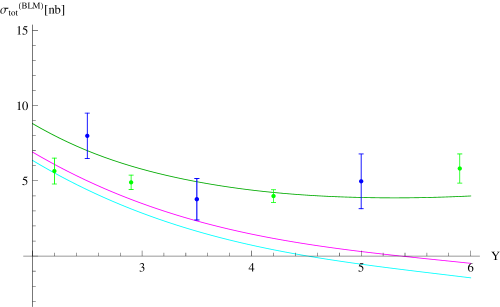
The results in this approach, calculated at s0=Q2subscript𝑠0superscript𝑄2s_{0}=Q^{2}, are shown in Fig. 6, where we can see that the cross section is very low and starts even to be negative at larger values of Y𝑌Y. In the same Figure, we show also the result obtained in Ref. [13] by a similar approach, but in the approximation where photon impact factors were taken at the LO.
Refer to caption
Figure 6: σtot(BLM,a)subscriptsuperscript𝜎BLMatot\sigma^{\rm(BLM,\ a)}_{\rm tot} (cyan line) and σtot(BLM,b)subscriptsuperscript𝜎BLMbtot\sigma^{\rm(BLM,\ b)}_{\rm tot} (magenta line) versus Y𝑌Y at Q2=17superscript𝑄217Q^{2}=17 GeV2 (nf=4subscript𝑛𝑓4n_{f}=4), together with the experimental data from OPAL (blue points, Q2=18superscript𝑄218Q^{2}=18 GeV2) and L3 (green points, Q2=16superscript𝑄216Q^{2}=16 GeV2); the green line represents the result of Ref. [13] (see Fig. 3 there).

4 Discussion

In this paper we have studied the γγsuperscript𝛾superscript𝛾\gamma^{*}\gamma^{*} total cross section in the NLA BFKL approach. First we have extracted the NLO corrections to the photon impact factor from two recent papers [15, 16], then we have used them to build several representations of the total cross section, equivalent within the NLA, but taking into account in a different way pieces of the (unknown) subleading contributions. We have combined these different representations with two among the most common methods for the optimization of a perturbative series, namely PMS and BLM, and compared their behavior with the energy with the only available experimental data, those from the LEP2 collider. We have considered also the numerical implementation of formulas describing the BFKL contribution to γγsuperscript𝛾superscript𝛾\gamma^{*}\gamma^{*} total cross section, derived originally by Chirilli and Kovchegov [16].

We have found that, in general, the effect of the BFKL resummation is small and changes only by little the determination coming from the LO quark box diagrams. This means that, in the considered range of energies, the NLO corrections to the photon impact factor compensate almost exactly the LO ones. Indeed, previous estimates of the cross section [11, 12, 13, 14] using LO impact factors together with the NLA BFKL Green’s function showed a better agreement with LEP2 data.

In other words, the account of the Balitsky and Chirilli expression for NLO photon impact factor reduces the BFKL contribution to the cross section to very small values making it impossible to describe LEP2 data as a sum of BFKL and LO QED quark box contributions. Note that, the LO QED quark box itself receives, at higher QCD orders, large corrections enhanced by double logs. Their resummation is important and leads to a considerable enhancement of the quark box contribution – see Ref. [4] for details, but still these effects are not large enough for a good description of LEP2 data at Y=3.5÷6𝑌3.56Y=3.5\div 6 without a sizable BFKL contribution.

There could be many reasons for this problem at Y=3.5÷6𝑌3.56Y=3.5\div 6. The first, obvious one, is that even at such high energies the BFKL contribution could be still not the dominant one in comparison with terms which are suppressed by powers of the energy 1/ssimilar-toabsent1𝑠\sim 1/s, and are not included in the present consideration. In particular, terms, subleading in energy, coming from diagrams with gluon exchange in the t𝑡t-channel, see Fig. 2, can be important. We could also argue that the presumably large effects in the next-to-NLA are not reduced under enough satisfactory control by the representations of the cross section and by the optimization methods we have considered in this work. In this respect, it would be interesting to test also approaches based on collinear improvement [30]. However, the consideration of these issues goes beyond the scope of present paper.
Refer to caption
Refer to caption
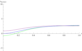
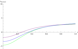
Figure 7: Behavior of rNLO/LOT(ν,s0,μR)superscriptsubscript𝑟NLOLO𝑇𝜈subscript𝑠0subscript𝜇𝑅r_{\rm NLO/LO}^{T}(\nu,s_{0},\mu_{R}) (green), rNLO/LOL(ν,s0,μR)superscriptsubscript𝑟NLOLO𝐿𝜈subscript𝑠0subscript𝜇𝑅r_{\rm NLO/LO}^{L}(\nu,s_{0},\mu_{R}) (blue) and rNLO/LO(mesons)(ν,s0,μR)superscriptsubscript𝑟NLOLOmesons𝜈subscript𝑠0subscript𝜇𝑅r_{\rm NLO/LO}^{(\rm mesons)}(\nu,s_{0},\mu_{R}) (violet) for the following cases: Q2=μR2=17superscript𝑄2superscriptsubscript𝜇𝑅217Q^{2}=\mu_{R}^{2}=17 GeV2, Y0=0subscript𝑌00Y_{0}=0 on the left and Q2=17superscript𝑄217Q^{2}=17 GeV2, μR2=(10Q)2superscriptsubscript𝜇𝑅2superscript10𝑄2\mu_{R}^{2}=(10Q)^{2}, Y0=2.2subscript𝑌02.2Y_{0}=2.2 on the right.

Definitely, the problems with our description of LEP2 data in the present context originate from the large negative value of NLO contributions to the photon impact factor. For this reason, we will discuss several issues related with this quantity. First, we want to illustrate our statement that the NLO corrections to the photon impact factor turned to be very large. For this purpose we plot in Fig. 7 the factors which, in the case of transverse and longitudinal photon polarizations, control the normalization of the cross section in the case of the exponential representation (23),

rNLO/LO(T,L)(ν,s0,μR)1+α¯s(μR)(FT,L(1)(ν,s0,μR)FT,L(ν)+FT,L(1)(ν,s0,μR)FT,L(ν)).superscriptsubscript𝑟NLOLO𝑇𝐿𝜈subscript𝑠0subscript𝜇𝑅1subscript¯𝛼𝑠subscript𝜇𝑅superscriptsubscript𝐹𝑇𝐿1𝜈subscript𝑠0subscript𝜇𝑅subscript𝐹𝑇𝐿𝜈superscriptsubscript𝐹𝑇𝐿1𝜈subscript𝑠0subscript𝜇𝑅subscript𝐹𝑇𝐿𝜈r_{\rm NLO/LO}^{(T,L)}(\nu,s_{0},\mu_{R})\equiv 1+\bar{\alpha}_{s}(\mu_{R})\left(\frac{F_{T,L}^{(1)}(\nu,s_{0},\mu_{R})}{F_{T,L}(\nu)}+\frac{F_{T,L}^{(1)}(-\nu,s_{0},\mu_{R})}{F_{T,L}(-\nu)}\right)\;. (32)

For the sake of comparison, we present in Fig. 7 also the similar quantity rNLO/LO(mesons)superscriptsubscript𝑟NLOLOmesonsr_{\rm NLO/LO}^{(\rm mesons)} which appeared in the description of the process γγsuperscript𝛾superscript𝛾\gamma^{*}\gamma^{*} to two light vector mesons, see Refs. [21, 22],

rNLO/LO(mesons)(ν,s0,μR)1+α¯s(μR)(c1(1)(ν,s0,μR)c1(ν)+c2(1)(ν,s0,μR)c2(ν)).superscriptsubscript𝑟NLOLOmesons𝜈subscript𝑠0subscript𝜇𝑅1subscript¯𝛼𝑠subscript𝜇𝑅superscriptsubscript𝑐11𝜈subscript𝑠0subscript𝜇𝑅subscript𝑐1𝜈superscriptsubscript𝑐21𝜈subscript𝑠0subscript𝜇𝑅subscript𝑐2𝜈r_{\rm NLO/LO}^{(\rm mesons)}(\nu,s_{0},\mu_{R})\equiv 1+\bar{\alpha}_{s}(\mu_{R})\left(\frac{c_{1}^{(1)}(\nu,s_{0},\mu_{R})}{c_{1}(\nu)}+\frac{c_{2}^{(1)}(-\nu,s_{0},\mu_{R})}{c_{2}(-\nu)}\right)\;. (33)

The ν𝜈\nu dependence of these quantities is shown on the left panel of Fig. 7 in the case of natural scale choice, s0=μR2=Q2subscript𝑠0superscriptsubscript𝜇𝑅2superscript𝑄2s_{0}=\mu_{R}^{2}=Q^{2}, whereas on the right panel we show the same quantities calculated for μR2=(10Q)2superscriptsubscript𝜇𝑅2superscript10𝑄2\mu_{R}^{2}=(10Q)^{2}, Y0=2.2subscript𝑌02.2Y_{0}=2.2, the values of scales which were obtained in Refs. [21, 22] during PMS optimization procedure applied to γγVVsuperscript𝛾superscript𝛾𝑉𝑉\gamma^{*}\gamma^{*}\to VV process. In the region of large-ν𝜈\nu the results are similar in all the three cases, whereas in the low-ν𝜈\nu region they differ substantially. For natural scales (left panel) and ν0.25𝜈0.25\nu\leq 0.25 all the three quantities are negative; note that it is the region of ν𝜈\nu that dominates the ν𝜈\nu-integral appearing in the cross section. We see that in this ν𝜈\nu-region the NLO corrections to the impact factors are negative and turn to be much larger for γγsuperscript𝛾superscript𝛾\gamma^{*}\to\gamma^{*} (especially in the case of transverse polarization) in comparison to the case of γVsuperscript𝛾𝑉\gamma^{*}\to V impact factor. Such a difference remains to be understood.

The impact factors in BFKL approach depend on the scales s0subscript𝑠0s_{0} and μRsubscript𝜇𝑅\mu_{R}, see Eqs. (2) and (2). Comparing the left and right panels of Fig. 7, one can see that this effect is important. In particular, γVsuperscript𝛾𝑉\gamma^{*}\to V and γLγLsuperscriptsubscript𝛾𝐿subscriptsuperscript𝛾𝐿\gamma_{L}^{*}\to\gamma^{*}_{L} impact factors become positive in the whole ν𝜈\nu range when one goes from the natural choice of scales to μR2=(10Q)2superscriptsubscript𝜇𝑅2superscript10𝑄2\mu_{R}^{2}=(10Q)^{2}, Y0=2.2subscript𝑌02.2Y_{0}=2.2. But it is not the case for the γTγTsuperscriptsubscript𝛾𝑇subscriptsuperscript𝛾𝑇\gamma_{T}^{*}\to\gamma^{*}_{T} impact factor, which remains negative-valued for a substantial range of small ν𝜈\nu. Note that the transverse polarization gives the most important contributions (σTTsubscript𝜎𝑇𝑇\sigma_{TT}) to the effective γγsuperscript𝛾superscript𝛾\gamma^{*}\gamma^{*} cross section which we consider in this paper. This observation explains, on the qualitative level, the very high values of optimal scales in Tables 1 and 2, which we found with PMS method for the γγsuperscript𝛾superscript𝛾\gamma^{*}\gamma^{*} total cross section.

The other issue we want to mention here is the color structure of the NLO parts of the photon impact factors. We observe that the NLO impact factors as extracted from [16] have very simple subleading 1/Nc2similar-toabsent1superscriptsubscript𝑁𝑐2\sim 1/N_{c}^{2} contributions, which appear only in the trivial third terms of Eqs. (2) and (2). This is in sharp contrast with what happens in the case of the NLO virtual photon to light vector meson impact factor [20] and of the NLO forward jet impact factor [23]. It would be interesting to understand the reason for the practically complete cancellation of the subleading 1/Nc21superscriptsubscript𝑁𝑐21/N_{c}^{2} terms which takes place here.

Finally, we want to compare the results for the photon impact factor which we used in this paper (derived from the results in [15, 16]) with the ones obtained in the conventional BFKL approach by Bartels and collaborators [10]. Unfortunately, some information (in numerical form) about the final result for the impact factor is available only for the case of transverse polarization – see Ref. [31] in the “Diffraction 2006” workshop proceedings. To make such a comparison we need to transfer the photon impact factor from the ν𝜈\nu- to the transverse momentum representation:

ΦT(x,s0,μR)=𝑑ν(x)iν+12π2[FT(ν)+α¯s(μR)FT(1)(ν,s0,μR)],subscriptΦ𝑇𝑥subscript𝑠0subscript𝜇𝑅subscriptsuperscriptdifferential-d𝜈superscript𝑥𝑖𝜈12𝜋2delimited-[]subscript𝐹𝑇𝜈subscript¯𝛼𝑠subscript𝜇𝑅superscriptsubscript𝐹𝑇1𝜈subscript𝑠0subscript𝜇𝑅\Phi_{T}(x,s_{0},\mu_{R})=\int\limits^{\infty}_{-\infty}d\nu\frac{(x)^{-i\nu+{1\over 2}}}{\pi\sqrt{2}}\left[F_{T}(\nu)+\bar{\alpha}_{s}(\mu_{R})F_{T}^{(1)}(\nu,s_{0},\mu_{R})\right]\,, (34)

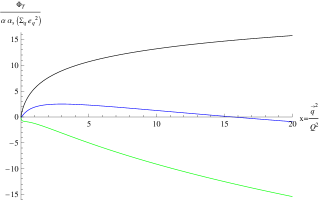
where the variable x𝑥x is defined as a dimensionless ratio of the Reggeon transverse momentum q𝑞\vec{q} and the photon virtuality squared: xq 2/Q2𝑥superscript𝑞2superscript𝑄2x\equiv\vec{q}^{\,2}/Q^{2}. The plot of ΦT(x,s0,μR)subscriptΦ𝑇𝑥subscript𝑠0subscript𝜇𝑅\Phi_{T}(x,s_{0},\mu_{R}) as a function of x𝑥x is presented in Fig. 6 of Ref. [31]. Here we perform the ν𝜈\nu integration in (34) using Eq. (2), the Balitsky-Chirilli result for the transverse photon impact factor transformed to the conventional BFKL scheme. In our Fig. 8 we present results for ΦT(x,s0,μR)/(ααs(qeq2))subscriptΦ𝑇𝑥subscript𝑠0subscript𝜇𝑅𝛼subscript𝛼𝑠subscript𝑞superscriptsubscript𝑒𝑞2\Phi_{T}(x,s_{0},\mu_{R})/(\alpha\,\alpha_{s}\left(\sum_{q}e_{q}^{2}\right)), where we used the following settings in order to compare with [31]: s0=10subscript𝑠010s_{0}=10 GeV2 , Q2=μR2=15superscript𝑄2superscriptsubscript𝜇𝑅215Q^{2}=\mu_{R}^{2}=15 GeV2; moreover, we take nf=1subscript𝑛𝑓1n_{f}=1 and αs=0.177206subscript𝛼𝑠0.177206\alpha_{s}=0.177206.222We are grateful to Grigorios Chachamis who provided us with the information about the numeric values of nfsubscript𝑛𝑓n_{f} and αssubscript𝛼𝑠\alpha_{s} which were used to produce Fig. 6 of [31]. In Fig. 8 we show the behavior of the photon impact factor with the Reggeon transverse momentum q𝑞\vec{q}, through the variable x𝑥x. In Fig. 8 the black curve represents the LO impact factor, the green curve gives LO plus NLO parts derived from Eq. (2), and the blue curve LO plus NLO parts derived from Eq. (2), when NLO contribution is reduced by the factor 1.87. We see that the NLO corrections are rather large and it is clear that the x𝑥x-shape of Φ(x,s0,μR)Φ𝑥subscript𝑠0subscript𝜇𝑅\Phi(x,s_{0},\mu_{R}) is rather sensitive to their value. Comparing the shape of the x𝑥x-dependence in Fig. 6 of [31] with the NLO curves in Fig. 8, we should conclude that the results of Balitsky and Chirilli are not in agreement with those presented in [31]. Interestingly, a qualitative agreement for the x𝑥x-shape of Φ(x,s0,μR)Φ𝑥subscript𝑠0subscript𝜇𝑅\Phi(x,s_{0},\mu_{R}) could be obtained only reducing the NLO result given in Eq.  (2) by the factor 1.87similar-toabsent1.87\sim 1.87.

To summarize this discussion we would like to stress that it would be very important if the authors of [31] could finally publish their results for the photon impact factor, since it would be an independent test of the results obtained by Balitsky and Chirilli using a completely different approach.
Refer to caption
Figure 8: Behavior of the photon impact factor (the transverse polarization) with the Reggeon transverse momentum q𝑞\vec{q}, through the variable xq 2/Q2𝑥superscript𝑞2superscript𝑄2x\equiv\vec{q}^{\,2}/Q^{2}. The black curve represents the LO impact factor, the green curve the sum of LO and NLO parts derived from Eq. (2) and the blue curve the same as the green curve, but with the NLO part reduced by the factor 1.87.

Acknowledgments

The authors are grateful to G. Chirilli and Yu. Kovchegov for valuable discussions. D.I. thanks the Dipartimento di Fisica dell’Università della Calabria and the Istituto Nazionale di Fisica Nucleare (INFN), Gruppo collegato di Cosenza, for warm hospitality and financial support. The work of D.I. was also supported in part by the grant RFBR-13-02-00695-a.
The work of B.M. was supported by the European Commission, European Social Fund and Calabria Region, that disclaim any liability for the use that can be done of the information provided in this paper.
B.M. thanks the Sobolev Institute of Mathematics of Novosibirsk for warm hospitality during the preparation of this work.

References

  • [1] V.M. Budnev, I.F. Ginzburg, G.V. Meledin, V.G. Serbo, Phys. Rept. 15 (1975) 181.
  • [2] I. Schienbein, Annals Phys. 301 (2002) 128.
  • [3] M. Cacciari, V. Del Duca, S. Frixione, Z. Trocsanyi, JHEP 0102 (2001) 029.
  • [4] J. Bartels, M. Lublinsky, JHEP 0309 (2003) 076; Mod. Phys. Lett. A 19 (2004) 19691982.
  • [5] V.S. Fadin, E.A. Kuraev, L.N. Lipatov, Phys. Lett. B 60 (1975) 50; E.A. Kuraev, L.N. Lipatov, V.S. Fadin, Zh. Eksp. Teor. Fiz. 71 (1976) 840 [Sov. Phys. JETP 44 (1976) 443]; 72 (1977) 377 [45 (1977) 199]; Ya.Ya. Balitskii, L.N. Lipatov, Sov. J. Nucl. Phys. 28 (1978) 822.
  • [6] F. Hautmann, OITS-613-96, C96-07-25; J. Bartels, A. De Roeck, H. Lotter, Phys. Lett. B 389 (1996) 742; A. Bialas, W. Czyz, W. Florkowski, Eur. Phys. J. C 2 (1998) 683; S.J. Brodsky, F. Hautmann, D.E. Soper, Phys. Rev. D 56 (1997) 6957; Phys. Rev. Lett. 78 (1997) 803 [Erratum-ibid. 79 (1997) 3544]; J. Kwiecinski, L. Motyka, Phys. Lett. B 462 (1999) 203; Eur. Phys. J. C 18 (2000) 343; M. Boonekamp, A. De Roeck, C. Royon, S. Wallon, Nucl. Phys. B 555 (1999) 540; J. Bartels, C. Ewerz, R. Staritzbichler, Phys. Lett. B 492 (2000) 56; N.N. Nikolaev, J. Speth, V.R. Zoller, Eur. Phys. J. C 22 (2002) 637; JETP 93 (2001) 957 [Zh. Eksp. Teor. Fiz. 93 (2001) 1104].
  • [7] V.S. Fadin, L.N. Lipatov, Phys. Lett. B 429 (1998) 127; M. Ciafaloni, G. Camici, Phys. Lett. B 430 (1998) 349.
  • [8] L.N. Lipatov, V.S. Fadin, Sov. J. Nucl. Phys. 50 (1989) 712; V.S. Fadin, R. Fiore, Phys. Lett. B 294 (1992) 286; V.S. Fadin, L.N. Lipatov, Nucl. Phys. B 406 (1993) 259; V.S. Fadin, R. Fiore, A. Quartarolo, Phys. Rev. D 50 (1994) 5893; V.S. Fadin, R. Fiore, M.I. Kotsky, Phys. Lett. B 359 (1995) 181; V.S. Fadin, R. Fiore, M.I. Kotsky, Phys. Lett. B 387 (1996) 593; V.S. Fadin, R. Fiore, M.I. Kotsky, Phys. Lett. B 389 (1996) 737; V.S. Fadin, R. Fiore, A. Quartarolo, Phys. Rev. D 53 (1996) 2729; V.S. Fadin, L.N. Lipatov, Nucl. Phys. B 477 (1996) 767; V.S. Fadin, M.I. Kotsky, L.N. Lipatov, Phys. Lett. B 415 (1997) 97; V.S. Fadin, R. Fiore, A. Flachi, M.I. Kotsky, Phys. Lett. B 422 (1998) 287; S. Catani, M. Ciafaloni, F. Hautmann, Phys. Lett. B 242 (1990) 97; G. Camici, M. Ciafaloni, Phys. Lett. B 386 (1996) 341; Nucl. Phys. B 496 (1997) 305.
  • [9] V.S. Fadin, hep-ph/9807528.
  • [10] J. Bartels, S. Gieseke, C.F. Qiao, Phys. Rev. D 63 (2001) 056014 [Erratum-ibid. D 65 (2002) 079902]; J. Bartels, S. Gieseke, A. Kyrieleis, Phys. Rev. D 65 (2002) 014006; J. Bartels, D. Colferai, S. Gieseke, A. Kyrieleis, Phys. Rev. D 66 (2002) 094017; J. Bartels, Nucl. Phys. (Proc. Suppl.) (2003) 116; J. Bartels, A. Kyrieleis, Phys. Rev. D 70 (2004) 114003; V.S. Fadin, D.Yu. Ivanov, M.I. Kotsky, Phys. Atom. Nucl. 65 (2002) 1513 [Yad. Fiz. 65 (2002) 1551]; Nucl. Phys. B 658 (2003) 156.
  • [11] S.J. Brodsky, V.S. Fadin, V.T. Kim, L.N. Lipatov, G.B. Pivovarov, JETP Lett. 76 (2002) 249 [Pisma Zh. Eksp. Teor. Fiz. 76 (2002) 306].
  • [12] S.J. Brodsky, V.S. Fadin, V.T. Kim, L.N. Lipatov, G.B. Pivovarov, JETP Lett. 70 (1999) 155.
  • [13] F. Caporale, D.Yu. Ivanov, A. Papa, Eur. Phys. J. C 58 (2008) 1-7.
  • [14] X.-C. Zheng, X.-G. Wu, S.-Q. Wang, J.-M. Shen, Q.-L. Zhang, JHEP 1310 (2013) 117.
  • [15] I. Balitsky, G.A. Chirilli, Phys. Rev. D 87 (2013) 014013.
  • [16] G.A. Chirilli, Yu.V. Kovchegov, JHEP 1405 (2014) 099.
  • [17] V.S. Fadin, R. Fiore, A. Papa, Phys. Lett. B 647 (2007) 179; Nucl. Phys. B 769 (2007) 108; V.S. Fadin, R. Fiore, A.V. Grabovsky, A. Papa, Nucl. Phys. B 784 (2007) 49.
  • [18] I. Balitsky, G.A. Chirilli, Phys. Lett. B 687 (2010) 204.
  • [19] G.A. Chirilli, Yu.V. Kovchegov, JHEP 1306 (2013) 055.
  • [20] D.Yu. Ivanov, M.I. Kotsky, A. Papa, Eur. Phys. J. C 38 (2004) 195-213.
  • [21] D.Yu. Ivanov, A. Papa, Nucl. Phys. B 732 (2006) 183-199; Eur. Phys. J. C 49 (2007) 947-955.
  • [22] F. Caporale, A. Sabio Vera, A. Papa, Eur. Phys. J. C 53 (2008) 525-532.
  • [23] J. Bartels, D. Colferai, G.P. Vacca, Eur. Phys. J. C 24 (2002) 83; Eur. Phys. J. C 29 (2003) 235; F. Caporale, D.Yu. Ivanov, B. Murdaca, A. Papa, A. Perri, JHEP 02 (2012) 101; D.Yu. Ivanov, A. Papa, JHEP 05 (2012) 086.
  • [24] D. Colferai, F. Schwennsen, L. Szymanowski, S. Wallon, JHEP 1012 (2010) 026; B. Ducloué, L. Szymanowski, S. Wallon, JHEP 1305 (2013) 096; F. Caporale, D.Yu. Ivanov, B. Murdaca, A. Papa, Nucl. Phys. B 877 (2013) 73; B. Ducloué, L. Szymanowski, S. Wallon, Phys. Rev. Lett. 112 (2014) 082003.
  • [25] P.M. Stevenson, Phys. Lett. B 100 (1981) 61; Phys. Rev. D 23 (1981) 2916.
  • [26] S.J. Brodsky, G.P. Lepage, P.B. Mackenzie, Phys. Rev. D 28 (1983) 228.
  • [27] P. Achard et al. [L3 Collaboration], Phys. Lett. B 531 (2002) 39.
  • [28] G. Abbiendi et al. [OPAL Collaboration], Eur. Phys. J. C 24 (2002) 17.
  • [29] F. Caporale, D.Yu. Ivanov, B. Murdaca, A. Papa, On the BLM optimal renormalization scale setting for semihard processes, in preparation.
  • [30] G.P. Salam, JHEP 9807 (1998) 019; M. Ciafaloni, D. Colferai, G.P. Salam, A.M. Stasto, Phys. Lett. B 587 (2004) 87; Phys. Rev. D 68 (2003) 114003; Phys. Lett. B 576 (2003) 143; Phys. Lett. B 541 (2002) 314; Phys. Rev. D 66 (2002) 054014; M. Ciafaloni, D. Colferai, G.P. Salam, JHEP 0007 (2000) 054; JHEP 9910 (1999) 017; Phys. Rev. D 60 (1999) 114036; M. Ciafaloni, D. Colferai, Phys. Lett. B 452 (1999) 372; A. Sabio Vera, Nucl. Phys. B 722 (2005) 65.
  • [31] G. Chachamis, J. Bartels, PoS DIFF 2006 (2006) 026.