Probability of Stability of Synchronization in Random Networks of Mismatched Oscillators

Saeed Manaffam,  and Alireza Seyedi The authors are with the Department of Electrical Engineering and Computer Science, University of Central Florida, Orlando, FL, 32816 USA e-mail: saeedmanaffam@knights.ucf.edu and alireza.seyedi@ieee.org.
Abstract

The stability of synchronization state in networks of oscillators are studied under the assumption that oscillators and their couplings have slightly mismatched parameters. A generalized master stability function is provided that takes the mismatches into account. Using this master stability function a lower bound on the probability of synchronization is derived for regular and random network models. The probability of stability of synchronization is then used to study the phase transition behavior of the networks. Numerical examples using van der Pol oscillators are used to illustrate the results and verify the validity of the analysis. Moreover, the synchronization trend as a function of statistics of mismatches in the coupling and local dynamics is investigated using this numerical example.

Index terms: Synchronization, random networks, Erdös-Rényi networks, small-world networks, probability of stability, parameter mismatch, van der Pol oscillator.

I Introduction

The problem of synchronization in a network of identical oscillators was first introduced by Wiener [1, 2]. Pursuit of the idea by Winfree in his pioneering work [3] led to this problem being recognized as being important and relevant in many fields of research including biology, physics, and engineering [4]. More recently, the introduction of the framework of master stability function by Pecora and Carroll [5], enabled the investigation of the impacts of network structure and the dynamical properties of individual nodes on the stability of the synchronization state [5, 6]. Following the idea of using master stability function to study the network of oscillators, most efforts have been concentrated on the impact of the topology (structure) of different types of networks on the stability of the synchronization state: In [5], the short and long wavelength bifurcation phenomena have been studied on regular networks (lattices). Other works look at linking the topological properties such as minimum, maximum and average node degrees, to the stability of the synchronization state in networks [6, 7, 8, 9]. Due to the interesting properties of small-world networks, which have been introduced in the seminal work of Watts and Strogatz [10, 11], most of the following studies were focused on the small-world and scale-free networks. It has been shown that due to better dynamical flow (efficient communications), the synchronization can be stabilized more easily in small-world networks compared to regular networks [2, 8, 12]. It has also been shown that the synchronizability of networks improves in homogeneous networks in contrast to heterogeneous ones [13].

Although the study of the synchronization of networks of the identical nodes appears to be matured, few attempts have been made to study networks with nonidentical nodes or couplings. The experiments reported in [14] suggest that in the networks where the oscillator dynamics and their couplings vary slightly from each other, the oscillators can be nearly synchronized. That is, the states converge to the vicinity of a certain trajectory (synchronization manifold). In [15] and [16], a sensitivity analysis of synchronization have been performed for a network of mismatched oscillators. It has been shown that near-synchronization behavior can occur in a network of mismatched oscillators using master stability function. The general stability of the synchronization in network of dynamical systems with nonidentical dynamics for each node is studied in [17] and [18] using the Lyapunov direct method. In [19], an approximate master stability function is proposed and the coupling strength is optimized to achieve “best synchronization properties”.

In this paper, we investigate the synchronization of a network of mismatched oscillators with mismatched couplings. Our formulation also allows the consideration of uncertainties in network link weights, thus generalizing [16] in addition to its main contributions. Since in presence of mismatch there is no unique synchronization state in the network, we use the concept of ε𝜀\varepsilon-synchronization [15], where the steady states of the nodes in the network fall into an ε𝜀\varepsilon-neighborhood of a certain trajectory (synchronization manifold). We then use a generalized master stability function to study the behavior of the network around the synchronization state. The proposed generalized master stability function bounds the oscillator states to a neighborhood of average synchronization trajectory as a function of Lyapunov exponents of the dynamical network. These Lyapunov exponents, in turn, are related to eigenvalues of the Laplacian matrix of the network. We then provide a probabilistic treatment of synchronization behavior in terms of mismatch parameters for regular and random network models. We calculate probability of stability of synchronization, and use it to investigate phase transitions of the synchronization in the network as the network and node parameters vary. Finally, we verify our analytical results by a numerical example for a network of van der Pol oscillators [20] with mismatched oscillators and couplings.

II Notation and Main Variables

The set of real (column) n𝑛n-vectors is denoted by nsuperscript𝑛\mathbb{{R}}^{n} and the set of real m×n𝑚𝑛m\times n matrices is denoted by m×nsuperscript𝑚𝑛\mathbb{{R}}^{m\times n}. We refer to the set of non-negative real numbers by +subscript\mathbb{{R}}_{+}. Matrices and vectors are denoted by capital and lower-case bold letters, respectively. Identity matrix is shown by I. The Euclidean (2subscript2\mathcal{L}_{2}) vector norm is represented by delimited-∥∥\lVert\cdot\rVert. When applied to a matrix, delimited-∥∥\lVert\cdot\rVert denotes the 2subscript2\mathcal{L}_{2} induced matrix norm, A=λmax(ATA)delimited-∥∥Asubscript𝜆superscriptA𝑇A\lVert\mbox{{\bf A}}\rVert=\sqrt{\lambda_{\max}(\mbox{{\bf A}}^{T}\mbox{{\bf A}})}. Table I summarizes the main variables used.

TABLE I: Main variables
Variable Description
xisubscriptx𝑖\mbox{{\bf x}}_{i} State vector of node i𝑖i
𝜸isubscript𝜸𝑖\mbox{$\boldsymbol{\gamma}$}_{i} Parameters vector of node i𝑖i
𝜽jisubscript𝜽𝑗𝑖\mbox{$\boldsymbol{\theta}$}_{ji} Parameter vector of coupling from node j𝑗j to node i𝑖i
𝐟(xi,𝜸i)𝐟subscriptx𝑖subscript𝜸𝑖\mathbf{f}(\mbox{{\bf x}}_{i},\mbox{$\boldsymbol{\gamma}$}_{i}) Dynamics function of node i𝑖i
h(xj,xi,𝜽ji)hsubscriptx𝑗subscriptx𝑖subscript𝜽𝑗𝑖\mbox{{\bf h}}(\mbox{{\bf x}}_{j},\mbox{{\bf x}}_{i},\mbox{$\boldsymbol{\theta}$}_{ji}) Coupling function from node j𝑗j to node i𝑖i
uisubscriptu𝑖\mbox{{\bf u}}_{i} Input vector for node i𝑖i
FxsubscriptFx\mbox{{\bf F}}_{\mbox{{\bf x}}} Jacobian of vector f with respect to x
F𝜸subscriptF𝜸\mbox{{\bf F}}_{\mbox{$\boldsymbol{\gamma}$}} Jacobian of vector f with respect to 𝜸𝜸\boldsymbol{\gamma}
HxsubscriptHx\mbox{{\bf H}}_{\mbox{{\bf x}}} Jacobian of coupling vector h with respect to x
HysubscriptHy\mbox{{\bf H}}_{\mbox{{\bf y}}} Jacobian of coupling vector h with respect to y
H𝜽subscriptH𝜽\mbox{{\bf H}}_{\mbox{$\boldsymbol{\theta}$}} Jacobian of coupling vector h with respect to 𝜽𝜽\boldsymbol{\theta}

III System Description

Consider a network of N𝑁N oscillators, indexed by 𝒩={1N}𝒩1𝑁\mbox{${\mathcal{N}}$}=\{1~{}\cdots~{}N\}. Assume that the dynamics of each isolated oscillator is governed by

x˙i=f(xi,𝜸i),subscript˙x𝑖fsubscriptx𝑖subscript𝜸𝑖\displaystyle\mbox{$\dot{\mbox{\bf x}}$}_{i}=\mbox{{\bf f}}(\mbox{{\bf x}}_{i},\mbox{$\boldsymbol{\gamma}$}_{i}),

where xinsubscriptx𝑖superscript𝑛\mbox{{\bf x}}_{i}\in\mathbb{{R}}^{n} and 𝜸i𝒫psubscript𝜸𝑖𝒫superscript𝑝\mbox{$\boldsymbol{\gamma}$}_{i}\in\mbox{${\mathcal{P}}$}\subseteq\mathbb{{R}}^{p} are the state and parameter vectors of local dynamics of node i𝑖i, respectively. 𝒫𝒫{\mathcal{P}} denotes the set of possible parameter vectors, and f:n+pn:fsuperscript𝑛𝑝superscript𝑛\mbox{{\bf f}}:\mathbb{{R}}^{n+p}\rightarrow\mathbb{{R}}^{n} describes the local dynamics of an isolated node.

The dynamics of coupled oscillators are given as

x˙isubscript˙x𝑖\displaystyle\mbox{$\dot{\mbox{\bf x}}$}_{i} =\displaystyle= f(xi,𝜸i)+i,j𝒩aijh(xj,xi,𝜽ij),fsubscriptx𝑖subscript𝜸𝑖subscript𝑖𝑗𝒩subscript𝑎𝑖𝑗hsubscriptx𝑗subscriptx𝑖subscript𝜽𝑖𝑗\displaystyle\mbox{{\bf f}}(\mbox{{\bf x}}_{i},\mbox{$\boldsymbol{\gamma}$}_{i})+\sum_{i,j\in\,\mbox{${\mathcal{N}}$}}a_{ij}\mbox{{\bf h}}(\mbox{{\bf x}}_{j},\,\mbox{{\bf x}}_{i},\,\mbox{$\boldsymbol{\theta}$}_{ij}), (1)

where 𝜽ij𝒬qsubscript𝜽𝑖𝑗𝒬superscript𝑞\mbox{$\boldsymbol{\theta}$}_{ij}\in\mbox{${\mathcal{Q}}$}\subseteq\mathbb{{R}}^{q} is the parameter vector of coupling dynamics from node j𝑗j to node i𝑖i, 𝒬𝒬{\mathcal{Q}} denotes the set of possible parameter values for couplings. The adjacency matrix of the network is A=[aij]Adelimited-[]subscript𝑎𝑖𝑗\mbox{{\bf A}}=[a_{ij}], where aij+subscript𝑎𝑖𝑗subscripta_{ij}\in\mathbb{{R}}_{+} is the weight of the link from node j𝑗j to node i𝑖i. There is no connection if aij=0subscript𝑎𝑖𝑗0a_{ij}=0. Note that we allow the more general case of directed and wighted networks. Moreover, h:2n+qn:hsuperscript2𝑛𝑞superscript𝑛\mbox{{\bf h}}:\mathbb{{R}}^{2n+q}\rightarrow\mathbb{{R}}^{n} models the coupling from node j𝑗j to node i𝑖i. We assume that h(x,y,𝜽)hxy𝜽\mbox{{\bf h}}(\mbox{{\bf x}},\mbox{{\bf y}},\mbox{$\boldsymbol{\theta}$}) is Hamiltonian. That is, we assume that Hx=HysubscriptHxsubscriptHy\mbox{{\bf H}}_{\mbox{{\bf x}}}=-\mbox{{\bf H}}_{\mbox{{\bf y}}}, where HxsubscriptHx\mbox{{\bf H}}_{\mbox{{\bf x}}} and HysubscriptHy\mbox{{\bf H}}_{\mbox{{\bf y}}} denotes the Jacobians of h(x,y,𝜽)hxy𝜽\mbox{{\bf h}}(\mbox{{\bf x}},\mbox{{\bf y}},\mbox{$\boldsymbol{\theta}$}) with respect to x and y, respectively. This is a very general assumption and encompasses the diffusive coupling model predominantly used in the literature [13, 16, 19], where it is assumed that h(x1,x2,[𝜽1𝜽2])=h~(x1,𝜽1)h~(x2,𝜽2)hsubscriptx1subscriptx2delimited-[]subscript𝜽1subscript𝜽2~hsubscriptx1subscript𝜽1~hsubscriptx2subscript𝜽2\mbox{{\bf h}}(\mbox{{\bf x}}_{1},\mbox{{\bf x}}_{2},[\mbox{$\boldsymbol{\theta}$}_{1}~{}\mbox{$\boldsymbol{\theta}$}_{2}])=\tilde{\mbox{{\bf h}}}(\mbox{{\bf x}}_{1},\mbox{$\boldsymbol{\theta}$}_{1})-\tilde{\mbox{{\bf h}}}(\mbox{{\bf x}}_{2},\mbox{$\boldsymbol{\theta}$}_{2}).

Note that this generalized model also incorporates uncertainties in the adjacency matrix of the network, A=[aij]+[δaij]Adelimited-[]subscript𝑎𝑖𝑗delimited-[]𝛿subscript𝑎𝑖𝑗\mbox{{\bf A}}=[a_{ij}]+[\delta a_{ij}], considered in [16], by absorbing δaij𝛿subscript𝑎𝑖𝑗\delta a_{ij} into θijsubscript𝜃𝑖𝑗\theta_{ij}, i.e., 𝜽ij=[𝜽ijTδaij]Tsubscriptsuperscript𝜽𝑖𝑗superscriptdelimited-[]superscriptsubscript𝜽𝑖𝑗𝑇𝛿subscript𝑎𝑖𝑗𝑇\mbox{$\boldsymbol{\theta}$}^{\prime}_{ij}=[\mbox{$\boldsymbol{\theta}$}_{ij}^{T}~{}\delta a_{ij}]^{T}.

IV Invariant Synchronization Manifold

Let s be a weighted average of the trajectories of all oscillators

s =\displaystyle= i𝒩αixi,subscript𝑖𝒩subscript𝛼𝑖subscriptx𝑖\displaystyle\sum_{i\in\,\mbox{${\mathcal{N}}$}}\alpha_{i}\mbox{{\bf x}}_{i}, (2)

where i𝒩αi=1subscript𝑖𝒩subscript𝛼𝑖1\sum_{i\in\,\mbox{${\mathcal{N}}$}}\alpha_{i}=1. Define the deviation of the trajectory of oscillator i𝑖i from s as

eisubscripte𝑖\displaystyle\mbox{{\bf e}}_{i} =\displaystyle= xis.subscriptx𝑖s\displaystyle\mbox{{\bf x}}_{i}-\mbox{{\bf s}}. (3)

Moreover, let L=[lij]Ldelimited-[]subscript𝑙𝑖𝑗\mbox{{\bf L}}=[l_{ij}] be the Laplacian matrix of the network [21],

L=diag([d1indNin])A,Ldiagdelimited-[]subscriptsuperscript𝑑in1subscriptsuperscript𝑑in𝑁A\mbox{{\bf L}}=\mbox{diag}([d^{\scriptsize\mbox{in}}_{1}\cdots d^{\scriptsize\mbox{in}}_{N}])-\mbox{{\bf A}},

where diin=j𝒩aijsuperscriptsubscript𝑑𝑖insubscript𝑗𝒩subscript𝑎𝑖𝑗d_{i}^{\scriptsize\mbox{in}}=\sum_{j\,\in\,\mbox{${\mathcal{N}}$}}a_{ij} is the in-degree of node i𝑖i.

Lemma 1.

s=i𝒩αixissubscript𝑖𝒩subscript𝛼𝑖subscriptx𝑖\mbox{{\bf s}}=\sum_{i\in\,\mbox{${\mathcal{N}}$}}\alpha_{i}\mbox{{\bf x}}_{i} is an invariant synchronization manifold of the network if 𝛂=[α1αN]T𝛂superscriptdelimited-[]subscript𝛼1subscript𝛼𝑁𝑇\mbox{$\boldsymbol{\alpha}$}=[\alpha_{1}\cdots\alpha_{N}]^{T} is a null vector of LTsuperscriptL𝑇\mbox{{\bf L}}^{T}.

Proof.

Taking derivative of (2) yields

s˙˙s\dot{\mbox{\bf s}} =\displaystyle= i𝒩αix˙isubscript𝑖𝒩subscript𝛼𝑖subscript˙x𝑖\displaystyle\sum_{i\,\in\,\mbox{${\mathcal{N}}$}}\alpha_{i}\mbox{$\dot{\mbox{\bf x}}$}_{i} (4)
=\displaystyle= i𝒩αif(s+ei,𝜸¯+δ𝜸i)subscript𝑖𝒩subscript𝛼𝑖fssubscripte𝑖bold-¯𝜸𝛿subscript𝜸𝑖\displaystyle\sum_{i\,\in\,\mbox{${\mathcal{N}}$}}\alpha_{i}\mbox{{\bf f}}(\mbox{{\bf s}}+\mbox{{\bf e}}_{i},\,\mbox{$\boldsymbol{\bar{\gamma}}$}+\delta\mbox{$\boldsymbol{\gamma}$}_{i})
+i,j𝒩aijαih(s+ej,s+ei,𝜽¯+δ𝜽ij),subscript𝑖𝑗𝒩subscript𝑎𝑖𝑗subscript𝛼𝑖hssubscripte𝑗ssubscripte𝑖bold-¯𝜽𝛿subscript𝜽𝑖𝑗\displaystyle+\sum_{i,j\in\,\mbox{${\mathcal{N}}$}}a_{ij}\alpha_{i}\mbox{{\bf h}}(\mbox{{\bf s}}+\mbox{{\bf e}}_{j},\,\mbox{{\bf s}}+\mbox{{\bf e}}_{i},\,\mbox{$\boldsymbol{\bar{\theta}}$}+\delta\mbox{$\boldsymbol{\theta}$}_{ij}),

where 𝜸¯=i𝒩αi𝜸ibold-¯𝜸subscript𝑖𝒩subscript𝛼𝑖subscript𝜸𝑖\mbox{$\boldsymbol{\bar{\gamma}}$}=\sum_{i\,\in\,\mbox{${\mathcal{N}}$}}\alpha_{i}\mbox{$\boldsymbol{\gamma}$}_{i}, δ𝜸i=𝜸i𝜸¯𝛿subscript𝜸𝑖subscript𝜸𝑖¯𝜸\delta\mbox{$\boldsymbol{\gamma}$}_{i}=\mbox{$\boldsymbol{\gamma}$}_{i}-\bar{\mbox{$\boldsymbol{\gamma}$}}, 𝜽¯=1d¯ini,j𝒩αiaij𝜽ijbold-¯𝜽1subscript¯𝑑insubscript𝑖𝑗𝒩subscript𝛼𝑖subscript𝑎𝑖𝑗subscript𝜽𝑖𝑗\mbox{$\boldsymbol{\bar{\theta}}$}=\frac{1}{\bar{d}_{\scriptsize\mbox{in}}}\sum_{i,j\,\in\,\mbox{${\mathcal{N}}$}}\alpha_{i}a_{ij}\mbox{$\boldsymbol{\theta}$}_{ij}, δ𝜽ij=𝜽ij𝜽¯𝛿subscript𝜽𝑖𝑗subscript𝜽𝑖𝑗¯𝜽\delta\mbox{$\boldsymbol{\theta}$}_{ij}=\mbox{$\boldsymbol{\theta}$}_{ij}-\bar{\mbox{$\boldsymbol{\theta}$}}, and d¯in=i𝒩αidiinsubscript¯𝑑insubscript𝑖𝒩subscript𝛼𝑖subscriptsuperscript𝑑in𝑖\bar{d}_{\scriptsize\mbox{in}}=\sum_{i\in\mbox{${\mathcal{N}}$}}\alpha_{i}d^{\scriptsize\mbox{in}}_{i} is the weighted average in-degree of the network. Linearization of (4) around (s,𝜸¯,𝜽¯)sbold-¯𝜸bold-¯𝜽(\mbox{{\bf s}},\,\mbox{$\boldsymbol{\bar{\gamma}}$},\,\mbox{$\boldsymbol{\bar{\theta}}$}) results in

s˙˙s\dot{\mbox{\bf s}} =\displaystyle= i𝒩αif(s,𝜸¯)+F𝜸i𝒩αiδ𝜸isubscript𝑖𝒩subscript𝛼𝑖fsbold-¯𝜸subscriptF𝜸subscript𝑖𝒩subscript𝛼𝑖𝛿subscript𝜸𝑖\displaystyle\sum_{i\,\in\,\mbox{${\mathcal{N}}$}}\alpha_{i}\mbox{{\bf f}}(\mbox{{\bf s}},\,\mbox{$\boldsymbol{\bar{\gamma}}$})+\mbox{{\bf F}}_{\mbox{$\boldsymbol{\gamma}$}}\sum_{i\,\in\mbox{${\mathcal{N}}$}}\alpha_{i}\delta\mbox{$\boldsymbol{\gamma}$}_{i}
+i,j𝒩aijαih(s,s,𝜽¯)+Hxi,j𝒩aijαi(ejei)subscript𝑖𝑗𝒩subscript𝑎𝑖𝑗subscript𝛼𝑖hssbold-¯𝜽subscriptHxsubscript𝑖𝑗𝒩subscript𝑎𝑖𝑗subscript𝛼𝑖subscripte𝑗subscripte𝑖\displaystyle+\sum_{i,\,j\in\,\mbox{${\mathcal{N}}$}}a_{ij}\alpha_{i}\mbox{{\bf h}}(\mbox{{\bf s}},\,\mbox{{\bf s}},\,\mbox{$\boldsymbol{\bar{\theta}}$})+\mbox{{\bf H}}_{\mbox{{\bf x}}}\sum_{i,\,j\in\,\mbox{${\mathcal{N}}$}}a_{ij}\alpha_{i}(\mbox{{\bf e}}_{j}-\mbox{{\bf e}}_{i})
+H𝜽i,j𝒩aijαiδ𝜽ji,subscriptH𝜽subscript𝑖𝑗𝒩subscript𝑎𝑖𝑗subscript𝛼𝑖𝛿subscript𝜽𝑗𝑖\displaystyle+\mbox{{\bf H}}_{\mbox{$\boldsymbol{\theta}$}}\sum_{i,\,j\in\,\mbox{${\mathcal{N}}$}}a_{ij}\alpha_{i}\delta\mbox{$\boldsymbol{\theta}$}_{ji},

where HxsubscriptHx\mbox{{\bf H}}_{\mbox{{\bf x}}} and H𝜽subscriptH𝜽\mbox{{\bf H}}_{\mbox{$\boldsymbol{\theta}$}} are Jacobians of h with respect to its first and third variable, respectively. Recalling that i𝒩αi=1subscript𝑖𝒩subscript𝛼𝑖1\sum_{i\in\,\mbox{${\mathcal{N}}$}}\alpha_{i}=1, we have

s˙˙s\dot{\mbox{\bf s}} =\displaystyle= f(s,𝜸¯)+h(s,s,𝜽¯)i𝒩diinαifsbold-¯𝜸hssbold-¯𝜽subscript𝑖𝒩subscriptsuperscript𝑑in𝑖subscript𝛼𝑖\displaystyle\mbox{{\bf f}}(\mbox{{\bf s}},\,\mbox{$\boldsymbol{\bar{\gamma}}$})+\mbox{{\bf h}}(\mbox{{\bf s}},\,\mbox{{\bf s}},\,\mbox{$\boldsymbol{\bar{\theta}}$})\sum_{i\,\in\,\mbox{${\mathcal{N}}$}}d^{\scriptsize\mbox{in}}_{i}\alpha_{i}
+Hxi,j𝒩aijαi(ejei).subscriptHxsubscript𝑖𝑗𝒩subscript𝑎𝑖𝑗subscript𝛼𝑖subscripte𝑗subscripte𝑖\displaystyle+\mbox{{\bf H}}_{\mbox{{\bf x}}}\sum_{i,j\in\,\mbox{${\mathcal{N}}$}}a_{ij}\alpha_{i}(\mbox{{\bf e}}_{j}-\mbox{{\bf e}}_{i}).

For s to be an invariant manifold, the last term in the above equation must be zero. This is achieved if αisubscript𝛼𝑖\alpha_{i} are chosen to satisfy

i,j𝒩aijαi(ejei)subscript𝑖𝑗𝒩subscript𝑎𝑖𝑗subscript𝛼𝑖subscripte𝑗subscripte𝑖\displaystyle\sum_{i,\,j\in\,\mbox{${\mathcal{N}}$}}a_{ij}\alpha_{i}(\mbox{{\bf e}}_{j}-\mbox{{\bf e}}_{i}) =\displaystyle= i𝒩[j𝒩(ajiαjaijαi)]eisubscript𝑖𝒩delimited-[]subscript𝑗𝒩subscript𝑎𝑗𝑖subscript𝛼𝑗subscript𝑎𝑖𝑗subscript𝛼𝑖subscripte𝑖\displaystyle\sum_{i\,\in\,\mbox{${\mathcal{N}}$}}\left[\sum_{j\,\in\,\mbox{${\mathcal{N}}$}}(a_{ji}\alpha_{j}-a_{ij}\alpha_{i})\right]\mbox{{\bf e}}_{i} (5)
=\displaystyle= 0.0\displaystyle\mbox{{\bf 0}}.

Equation (5), in turn, will be satisfied if j𝒩(aijαjaijαi)=0subscript𝑗𝒩subscript𝑎𝑖𝑗subscript𝛼𝑗subscript𝑎𝑖𝑗subscript𝛼𝑖0\sum_{j\,\in\,\mbox{${\mathcal{N}}$}}(a_{ij}\alpha_{j}-a_{ij}\alpha_{i})=0 for all i𝒩𝑖𝒩i\,\in\,\mbox{${\mathcal{N}}$}, which in matrix form can be represented as

AT𝜶=diag([d1indNin])𝜶,superscriptA𝑇𝜶diagdelimited-[]subscriptsuperscript𝑑in1subscriptsuperscript𝑑in𝑁𝜶\mbox{{\bf A}}^{T}\mbox{$\boldsymbol{\alpha}$}=\mbox{diag}([d^{\scriptsize\mbox{in}}_{1}\cdots d^{\scriptsize\mbox{in}}_{N}])\mbox{$\boldsymbol{\alpha}$},

where 𝜶=[α1αN]𝜶delimited-[]subscript𝛼1subscript𝛼𝑁\mbox{$\boldsymbol{\alpha}$}=[\alpha_{1}\cdots\alpha_{N}], or

[ATdiag([d1indNin])]𝜶=0=LT𝜶.delimited-[]superscriptA𝑇diagdelimited-[]subscriptsuperscript𝑑in1subscriptsuperscript𝑑in𝑁𝜶0superscriptL𝑇𝜶\left[\mbox{{\bf A}}^{T}-\mbox{diag}([d^{\scriptsize\mbox{in}}_{1}\cdots d^{\scriptsize\mbox{in}}_{N}])\right]\mbox{$\boldsymbol{\alpha}$}=\mbox{{\bf 0}}=\mbox{{\bf L}}^{T}\mbox{$\boldsymbol{\alpha}$}.

That is, 𝜶𝜶\boldsymbol{\alpha} is a null vector of LTsuperscriptL𝑇\mbox{{\bf L}}^{T}. ∎

Remark 1.

We note that, by definition, L has zero row sum. Thus, it is singular. Consequently, LTsuperscriptL𝑇\mbox{{\bf L}}^{T} always has a null vector, 𝛂𝛂\boldsymbol{\alpha}. This means that any network has at least one invariant manifold.

Remark 2.

If the the network is connected, the invariant synchronization manifold is unique. This is due to the fact that for connected networks the nullity of L is one. Thus, 𝛂𝛂\boldsymbol{\alpha} and, therefore, s are unique.

Remark 3.

In the special case where the network is undirected, L is symmetric. Thus, it also has zero column-sum. Consequently, 𝛂=1N[11]𝛂1𝑁delimited-[]11\mbox{$\boldsymbol{\alpha}$}=\frac{1}{N}[1~{}\cdots~{}1] is its null vector, and the invariant manifold, s, is the simple average of the trajectories.

With αisubscript𝛼𝑖\alpha_{i} chosen such that s is an invariant manifold, we have

s˙˙s\dot{\mbox{\bf s}} =\displaystyle= f(s,𝜸¯)+d¯inh(s,s,𝜽¯),fsbold-¯𝜸subscript¯𝑑inhssbold-¯𝜽\displaystyle\mbox{{\bf f}}(\mbox{{\bf s}},\,\mbox{$\boldsymbol{\bar{\gamma}}$})+\bar{d}_{\scriptsize\mbox{in}}\,\mbox{{\bf h}}(\mbox{{\bf s}},\,\mbox{{\bf s}},\,\mbox{$\boldsymbol{\bar{\theta}}$}), (6)
s(0)s0\displaystyle\mbox{{\bf s}}({0}) =\displaystyle= i𝒩αixi(0),subscript𝑖𝒩subscript𝛼𝑖subscriptx𝑖0\displaystyle\sum_{i\,\in\,\mbox{${\mathcal{N}}$}}\alpha_{i}\mbox{{\bf x}}_{i}({0}),

where s(0)s0\mbox{{\bf s}}(0) and x(0)x0\mbox{{\bf x}}({0}) are initial states.

V Generalized Master Stability Function

In this section we introduce a master stability function which generalizes those in [15] and [16] by taking into account the parameter mismatch in the links and applies to directed and weighted networks.

As it has been shown in previous section, every connected network has a unique invariant manifold. Hence, we can define ε𝜀\varepsilon-synchronization as

Definition 1.

A network of oscillators is ε𝜀\varepsilon-synchronized if there exists ε>0𝜀0\varepsilon>0 such that

lim supteε,subscriptlimit-supremum𝑡delimited-∥∥e𝜀\displaystyle\limsup_{t\to\infty}\lVert\mbox{{\bf e}}\rVert\leq\varepsilon,

where e=[e1eN]Tesuperscriptdelimited-[]subscripte1subscripte𝑁𝑇\mbox{{\bf e}}=[\mbox{{\bf e}}_{1}~{}...~{}\mbox{{\bf e}}_{N}]^{T}.

This definition means that the error from the manifold is contained in a ball of radius ε𝜀\varepsilon. We note that our definition is different but closely related to that given in [18].

Substituting (1) and (2) in (3), and using Taylor series, the dynamics of the error with respect to the synchronization manifold, eisubscripte𝑖\mbox{{\bf e}}_{i}, is given by

e˙isubscript˙e𝑖\displaystyle\mbox{$\dot{\mbox{\bf e}}$}_{i} =\displaystyle= Fxeij=1NlijHxej+F𝜸δ𝜸i+j=1N𝟙ijlijH𝜽δ𝜽ijsubscriptFxsubscripte𝑖superscriptsubscript𝑗1𝑁subscript𝑙𝑖𝑗subscriptHxsubscripte𝑗subscriptF𝜸𝛿subscript𝜸𝑖superscriptsubscript𝑗1𝑁subscript1𝑖𝑗subscript𝑙𝑖𝑗subscriptH𝜽𝛿subscript𝜽𝑖𝑗\displaystyle\mbox{{\bf F}}_{\mbox{{\bf x}}}\mbox{{\bf e}}_{i}-\sum_{j=1}^{N}l_{ij}\mbox{{\bf H}}_{\mbox{{\bf x}}}\mbox{{\bf e}}_{j}+\mbox{{\bf F}}_{\mbox{$\boldsymbol{\gamma}$}}\delta\mbox{$\boldsymbol{\gamma}$}_{i}+\sum_{j=1}^{N}\mathbbm{1}_{i\neq j}l_{ij}\mbox{{\bf H}}_{\mbox{$\boldsymbol{\theta}$}}\delta\mbox{$\boldsymbol{\theta}$}_{ij} (7)
+(diind¯in)h(s,s,𝜽¯),superscriptsubscript𝑑𝑖insubscript¯𝑑inhssbold-¯𝜽\displaystyle+(d_{i}^{\scriptsize\mbox{in}}-\bar{d}_{\scriptsize\mbox{in}})\mbox{{\bf h}}(\mbox{{\bf s}},\,\mbox{{\bf s}},\,\mbox{$\boldsymbol{\bar{\theta}}$}),

where 𝟙Xsubscript1𝑋\mathbbm{1}_{X} is the indicator function of X𝑋X. Stacking (7) for all i𝑖i yields the dynamics of the deviation of node trajectories from s:

e˙˙e\displaystyle\dot{\mbox{{\bf e}}} =\displaystyle= (IFxLHx)δx+(IF𝜸)δ𝜸tensor-productIsubscriptFxtensor-productLsubscriptHx𝛿xtensor-productIsubscriptF𝜸𝛿𝜸\displaystyle\left(\mbox{{\bf I}}\otimes\mbox{{\bf F}}_{\mbox{{\bf x}}}-\mbox{{\bf L}}\otimes\mbox{{\bf H}}_{\mbox{{\bf x}}}\right)\delta\mbox{{\bf x}}+\left(\mbox{{\bf I}}\otimes\mbox{{\bf F}}_{\mbox{$\boldsymbol{\gamma}$}}\right)\delta\mbox{$\boldsymbol{\gamma}$} (8)
+(𝓐H𝜽)δ𝜽+(dind¯in𝟏NT)h(s,s,𝜽¯),tensor-product𝓐subscriptH𝜽𝛿𝜽tensor-productsuperscriptdinsubscript¯𝑑insubscriptsuperscript1𝑇𝑁hssbold-¯𝜽\displaystyle+\left(\boldsymbol{\mathcal{A}}\otimes\mbox{{\bf H}}_{\mbox{$\boldsymbol{\theta}$}}\right)\delta\mbox{$\boldsymbol{\theta}$}+(\mbox{{\bf d}}^{\scriptsize\mbox{in}}-\bar{d}_{\scriptsize\mbox{in}}\mathbf{1}^{T}_{N})\otimes\mbox{{\bf h}}(\mbox{{\bf s}},\,\mbox{{\bf s}},\,\mbox{$\boldsymbol{\bar{\theta}}$}),

where

δ𝜸𝛿𝜸\displaystyle{\delta\mbox{$\boldsymbol{\gamma}$}} =\displaystyle= [δ𝜸1Tδ𝜸NT]T,superscriptdelimited-[]𝛿superscriptsubscript𝜸1𝑇𝛿superscriptsubscript𝜸𝑁𝑇𝑇\displaystyle[\delta\mbox{$\boldsymbol{\gamma}$}_{1}^{T}\cdots\delta\mbox{$\boldsymbol{\gamma}$}_{N}^{T}]^{T},
δ𝜽𝛿𝜽\displaystyle{\delta\mbox{$\boldsymbol{\theta}$}} =\displaystyle= [δ𝜽11Tδ𝜽1NTδ𝜽21Tδ𝜽2NT𝜽N1Tδ𝜽NNT]T,superscriptdelimited-[]𝛿superscriptsubscript𝜽11𝑇𝛿superscriptsubscript𝜽1𝑁𝑇𝛿superscriptsubscript𝜽21𝑇𝛿superscriptsubscript𝜽2𝑁𝑇superscriptsubscript𝜽𝑁1𝑇𝛿superscriptsubscript𝜽𝑁𝑁𝑇𝑇\displaystyle[\delta\mbox{$\boldsymbol{\theta}$}_{11}^{T}\cdots\delta\mbox{$\boldsymbol{\theta}$}_{1N}^{T}~{}\delta\mbox{$\boldsymbol{\theta}$}_{21}^{T}\cdots\delta\mbox{$\boldsymbol{\theta}$}_{2N}^{T}~{}\cdots~{}\mbox{$\boldsymbol{\theta}$}_{N1}^{T}\cdots\delta\mbox{$\boldsymbol{\theta}$}_{NN}^{T}]^{T},
dinsuperscriptdin\displaystyle\mbox{{\bf d}}^{\scriptsize\mbox{in}} =\displaystyle= [d1indNin]T,superscriptdelimited-[]superscriptsubscript𝑑1insuperscriptsubscript𝑑𝑁in𝑇\displaystyle[d_{1}^{\scriptsize\mbox{in}}\cdots d_{N}^{\scriptsize\mbox{in}}]^{T},
𝓐𝓐\displaystyle\boldsymbol{\mathcal{A}} =\displaystyle= diag([a1aN]),diagdelimited-[]subscripta1subscripta𝑁\displaystyle\mbox{diag}([\mbox{{\bf a}}_{1}\cdots\mbox{{\bf a}}_{N}]),

and aisubscripta𝑖\mbox{{\bf a}}_{i} is the i𝑖ith row of A.

Let L=PJP1LsuperscriptPJP1\mbox{{\bf L}}=\mbox{{\bf P}}\mbox{{\bf J}}\mbox{{\bf P}}^{-1} be the Jordan decomposition of L, where P=[pij]Pdelimited-[]subscript𝑝𝑖𝑗\mbox{{\bf P}}=[p_{ij}] is a similarity transform and J is in Jordan form. Then, (8) can be rewritten as

e˙˙e\displaystyle\dot{\mbox{{\bf e}}} =\displaystyle= (PI)(IFxJHx)(P1I)e+(IF𝜸)δ𝜸tensor-productPItensor-productIsubscriptFxtensor-productJsubscriptHxtensor-productsuperscriptP1Ietensor-productIsubscriptF𝜸𝛿𝜸\displaystyle\left(\mbox{{\bf P}}\otimes\mbox{{\bf I}}\right)\left(\mbox{{\bf I}}\otimes\mbox{{\bf F}}_{\mbox{{\bf x}}}-\mbox{{\bf J}}\otimes\mbox{{\bf H}}_{\mbox{{\bf x}}}\right)\left(\mbox{{\bf P}}^{-1}\otimes\mbox{{\bf I}}\right)\mbox{{\bf e}}+\left(\mbox{{\bf I}}\otimes\mbox{{\bf F}}_{\mbox{$\boldsymbol{\gamma}$}}\right){\delta\mbox{$\boldsymbol{\gamma}$}}
+(𝓐H𝜽)δ𝜽+(dind¯in𝟏NT)h(s,s,𝜽¯).tensor-product𝓐subscriptH𝜽𝛿𝜽tensor-productsuperscriptdinsubscript¯𝑑insuperscriptsubscript1𝑁𝑇hssbold-¯𝜽\displaystyle+\left(\boldsymbol{\mathcal{A}}\otimes\mbox{{\bf H}}_{\mbox{$\boldsymbol{\theta}$}}\right){\delta\mbox{$\boldsymbol{\theta}$}}+(\mbox{{\bf d}}^{\scriptsize\mbox{in}}-\bar{d}_{\scriptsize\mbox{in}}\mathbf{1}_{N}^{T})\otimes\mbox{{\bf h}}(\mbox{{\bf s}},\,\mbox{{\bf s}},\,\mbox{$\boldsymbol{\bar{\theta}}$}).

Using the similarity transform

𝜼=(P1I)e,𝜼tensor-productsuperscriptP1Ie\mbox{$\boldsymbol{\eta}$}=\left(\mbox{{\bf P}}^{-1}\otimes\mbox{{\bf I}}\right)\mbox{{\bf e}},

where 𝜼=[𝜼1T𝜼NT]T𝜼superscriptdelimited-[]subscriptsuperscript𝜼𝑇1superscriptsubscript𝜼𝑁𝑇𝑇\mbox{$\boldsymbol{\eta}$}=[\mbox{$\boldsymbol{\eta}$}^{T}_{1}\cdots\mbox{$\boldsymbol{\eta}$}_{N}^{T}]^{T}, we obtain

𝜼˙˙𝜼\displaystyle\dot{\mbox{$\boldsymbol{\eta}$}} =\displaystyle= (IFxJHx)𝜼+(P1I)(IF𝜸)δ𝜸tensor-productIsubscriptFxtensor-productJsubscriptHx𝜼tensor-productsuperscriptP1Itensor-productIsubscriptF𝜸𝛿𝜸\displaystyle\left(\mbox{{\bf I}}\otimes\mbox{{\bf F}}_{\mbox{{\bf x}}}-\mbox{{\bf J}}\otimes\mbox{{\bf H}}_{\mbox{{\bf x}}}\right)\mbox{$\boldsymbol{\eta}$}+\left(\mbox{{\bf P}}^{-1}\otimes\mbox{{\bf I}}\right)\left(\mbox{{\bf I}}\otimes\mbox{{\bf F}}_{\mbox{$\boldsymbol{\gamma}$}}\right){\delta\mbox{$\boldsymbol{\gamma}$}} (9)
+(P1I)(𝓐H𝜽)δ𝜽tensor-productsuperscriptP1Itensor-product𝓐subscriptH𝜽𝛿𝜽\displaystyle+\left(\mbox{{\bf P}}^{-1}\otimes\mbox{{\bf I}}\right)\left(\boldsymbol{\mathcal{A}}\otimes\mbox{{\bf H}}_{\mbox{$\boldsymbol{\theta}$}}\right){\delta\mbox{$\boldsymbol{\theta}$}}
+(P1I)((dd¯in𝟏NT)h(s,s,𝜽¯))tensor-productsuperscriptP1Itensor-productdsubscript¯𝑑insuperscriptsubscript1𝑁𝑇hssbold-¯𝜽\displaystyle+\left(\mbox{{\bf P}}^{-1}\otimes\mbox{{\bf I}}\right)\left((\mbox{{\bf d}}-\bar{d}_{\scriptsize\mbox{in}}\mathbf{1}_{N}^{T})\otimes\mbox{{\bf h}}(\mbox{{\bf s}},\,\mbox{{\bf s}},\,\mbox{$\boldsymbol{\bar{\theta}}$})\right)
=\displaystyle= (IFxJHx)𝜼+(P1F𝜸)δ𝜸tensor-productIsubscriptFxtensor-productJsubscriptHx𝜼tensor-productsuperscriptP1subscriptF𝜸𝛿𝜸\displaystyle\left(\mbox{{\bf I}}\otimes\mbox{{\bf F}}_{\mbox{{\bf x}}}-\mbox{{\bf J}}\otimes\mbox{{\bf H}}_{\mbox{{\bf x}}}\right)\mbox{$\boldsymbol{\eta}$}+\left(\mbox{{\bf P}}^{-1}\otimes\mbox{{\bf F}}_{\mbox{$\boldsymbol{\gamma}$}}\right){\delta\mbox{$\boldsymbol{\gamma}$}}
+(P1𝓐H𝜽)δ𝜽tensor-productsuperscriptP1𝓐subscriptH𝜽𝛿𝜽\displaystyle+\left(\mbox{{\bf P}}^{-1}\boldsymbol{\mathcal{A}}\otimes\mbox{{\bf H}}_{\mbox{$\boldsymbol{\theta}$}}\right){\delta\mbox{$\boldsymbol{\theta}$}}
+(P1(dd¯in𝟏NT))h(s,s,𝜽¯).tensor-productsuperscriptP1dsubscript¯𝑑insubscriptsuperscript1𝑇𝑁hssbold-¯𝜽\displaystyle+\left(\mbox{{\bf P}}^{-1}(\mbox{{\bf d}}-\bar{d}_{\scriptsize\mbox{in}}\mathbf{1}^{T}_{N})\right)\otimes\mbox{{\bf h}}(\mbox{{\bf s}},\,\mbox{{\bf s}},\,\mbox{$\boldsymbol{\bar{\theta}}$}).
=\displaystyle= (IFxJHx)𝜼+v,tensor-productIsubscriptFxtensor-productJsubscriptHx𝜼v\displaystyle\left(\mbox{{\bf I}}\otimes\mbox{{\bf F}}_{\mbox{{\bf x}}}-\mbox{{\bf J}}\otimes\mbox{{\bf H}}_{\mbox{{\bf x}}}\right)\mbox{$\boldsymbol{\eta}$}+\mbox{{\bf v}},

where v=[v1vN]vdelimited-[]subscriptv1subscriptv𝑁\mbox{{\bf v}}=[\mbox{{\bf v}}_{1}\cdots\mbox{{\bf v}}_{N}],

visubscriptv𝑖\displaystyle\mbox{{\bf v}}_{i} =\displaystyle= j𝒩qij[F𝜸δ𝜸j+k=1,kjNajkH𝜽δ𝜽jk\displaystyle\sum_{j\,\in\,\mbox{${\mathcal{N}}$}}q_{ij}\Bigg{[}\mbox{{\bf F}}_{\mbox{$\boldsymbol{\gamma}$}}\delta\mbox{$\boldsymbol{\gamma}$}_{j}+\sum_{k=1,k\neq j}^{N}a_{jk}\mbox{{\bf H}}_{\mbox{$\boldsymbol{\theta}$}}\delta\mbox{$\boldsymbol{\theta}$}_{jk}
+h(s,s,𝜽¯)(diind¯in)],\displaystyle+\mbox{{\bf h}}(\mbox{{\bf s}},\,\mbox{{\bf s}},\,\mbox{$\boldsymbol{\bar{\theta}}$})(d_{i}^{\scriptsize\mbox{in}}-\bar{d}_{\scriptsize\mbox{in}})\Bigg{]},

and qijsubscript𝑞𝑖𝑗q_{ij} are the elements of Q=P1QsuperscriptP1\mbox{{\bf Q}}=\mbox{{\bf P}}^{-1}. It is clear that stability of 𝜼𝜼\boldsymbol{\eta} and e are equivalent.

To study the stability of (9), let us first consider the simpler case where J consists of a single Jordan block, i.e.

J=JN(μ)=[μ10000μ10000μ00000μ10000μ].JsubscriptJ𝑁𝜇delimited-[]𝜇10000𝜇10000𝜇00000𝜇10000𝜇\displaystyle\mbox{{\bf J}}=\mbox{{\bf J}}_{N}(\mu)=\left[\begin{array}[]{cccccc}\mu&1&0&\cdots&0&0\\ 0&\mu&1&\cdots&0&0\\ 0&0&\mu&\cdots&0&0\\ \vdots&\vdots&\vdots&\ddots&\vdots&\vdots\\ 0&0&0&\cdots&\mu&1\\ 0&0&0&\cdots&0&\mu\end{array}\right]. (16)
Lemma 2.

For system

𝜼˙=(IFxJN(μ)Hx)𝜼+v,˙𝜼tensor-productIsubscriptFxtensor-productsubscriptJ𝑁𝜇subscriptHx𝜼v\displaystyle\dot{\mbox{$\boldsymbol{\eta}$}}=\left(\mbox{{\bf I}}\otimes\mbox{{\bf F}}_{\mbox{{\bf x}}}-\mbox{{\bf J}}_{N}(\mu)\otimes\mbox{{\bf H}}_{\mbox{{\bf x}}}\right)\mbox{$\boldsymbol{\eta}$}+\mbox{{\bf v}},

there exists ϕ>0italic-ϕ0\phi>0 such that

lim supt𝜼ij=iN(ϕλ)Nj+1lim suptFxHxNjsubscriptlimit-supremum𝑡delimited-∥∥subscript𝜼𝑖superscriptsubscript𝑗𝑖𝑁superscriptitalic-ϕ𝜆𝑁𝑗1subscriptlimit-supremum𝑡superscriptdelimited-∥∥subscriptFxsubscriptHx𝑁𝑗\displaystyle\limsup_{t\to\infty}\lVert\mbox{$\boldsymbol{\eta}$}_{i}\rVert\leq\sum_{j=i}^{N}\left(\frac{\phi}{\lambda}\right)^{N-j+1}\limsup_{t\to\infty}\lVert\mbox{{\bf F}}_{\mbox{{\bf x}}}-\mbox{{\bf H}}_{\mbox{{\bf x}}}\rVert^{N-j}
×lim suptvj,\displaystyle\times\limsup_{t\to\infty}\lVert\mbox{{\bf v}}_{j}\rVert,

for all i𝑖i, if λ>0𝜆0\lambda>0, where λ=MLE(FxμHx)𝜆MLEsubscriptFx𝜇subscriptHx\lambda=\mbox{MLE}(\mbox{{\bf F}}_{\mbox{{\bf x}}}-\mu\mbox{{\bf H}}_{\mbox{{\bf x}}}), and MLE(.)\mbox{MLE}(.) returns the maximum Lyapunov exponent of the argument.

Proof.

See Appendix A. ∎

Now, let us assume that J consists of M𝑀M Jordan blocks with eigenvalues μmsubscript𝜇𝑚\mu_{m} and sizes nm,m{1,,M}subscript𝑛𝑚𝑚1𝑀n_{m},~{}m\in\{1,\cdots,M\}, where m=1Mnm=Nsuperscriptsubscript𝑚1𝑀subscript𝑛𝑚𝑁\sum_{m=1}^{M}n_{m}=N. Then Nm=m=1jnmsubscript𝑁𝑚superscriptsubscript𝑚1𝑗subscript𝑛𝑚N_{m}=\sum_{m=1}^{j}n_{m} will be the index of the last row of the m𝑚mth Jordan block. Define J(i)𝐽𝑖J(i) to be the index of the Jordan block that contains the i𝑖ith row of J. In other words, J(i)=m𝐽𝑖𝑚J(i)=m, if Nm1<iNmsubscript𝑁𝑚1𝑖subscript𝑁𝑚N_{m-1}<i\leq N_{m}.

Theorem 1.

A network of oscillators is ε𝜀\varepsilon-synchronized if λm=MLE(FxμmHx)>0subscript𝜆𝑚MLEsubscriptFxsubscript𝜇𝑚subscriptHx0\lambda_{m}=\mbox{MLE}(\mbox{{\bf F}}_{\mbox{{\bf x}}}-\mu_{m}\mbox{{\bf H}}_{\mbox{{\bf x}}})>0 and

P2j=1N1(k=1nJ(j)(ϕJ(j)λJ(j))nJ(j)k+1\displaystyle\|\mbox{{\bf P}}\|^{2}\sum_{j=1}^{N-1}\Bigg{(}\sum_{k=1}^{n_{J(j)}}\left(\frac{\phi_{J(j)}}{\lambda_{J(j)}}\right)^{n_{J(j)}-k+1}\quad\quad\quad\quad\quad\quad\quad
×lim suptFxHxnJ(j)klim suptvj)2ε2,\displaystyle\times\limsup_{t\to\infty}\lVert\mbox{{\bf F}}_{\mbox{{\bf x}}}-\mbox{{\bf H}}_{\mbox{{\bf x}}}\rVert^{n_{\scriptsize J(j)}-k}\limsup_{t\to\infty}\lVert\mbox{{\bf v}}_{j}\rVert\bigg{)}^{2}\leq{\varepsilon}^{2}, (17)

where ϕmsubscriptitalic-ϕ𝑚\phi_{m} satisfies

t,τ,𝚽m(t,τ)ϕmeλm(tτ).for-all𝑡𝜏normsubscript𝚽𝑚𝑡𝜏subscriptitalic-ϕ𝑚superscript𝑒subscript𝜆𝑚𝑡𝜏\displaystyle\forall t,\tau,\quad\|\mathbf{\Phi}_{m}(t,\tau)\|\leq\phi_{m}e^{-\lambda_{m}(t-\tau)}.

and 𝚽m(t,τ)subscript𝚽𝑚𝑡𝜏\mathbf{\Phi}_{m}(t,\tau) is the state transition matrix of FxμmHxsubscriptFxsubscript𝜇𝑚subscriptHx\mbox{{\bf F}}_{\mbox{{\bf x}}}-\mu_{m}\mbox{{\bf H}}_{\mbox{{\bf x}}}.

Proof.

We have

lim supte2subscriptlimit-supremum𝑡superscriptdelimited-∥∥e2\displaystyle\limsup_{t\rightarrow\infty}\lVert\mbox{{\bf e}}\rVert^{2} =\displaystyle= lim supt𝜼T(PTI)(PI)𝜼subscriptlimit-supremum𝑡superscript𝜼𝑇tensor-productsuperscriptP𝑇Itensor-productPI𝜼\displaystyle\limsup_{t\to\infty}\mbox{$\boldsymbol{\eta}$}^{T}(\mbox{{\bf P}}^{T}\otimes\mbox{{\bf I}})(\mbox{{\bf P}}\otimes\mbox{{\bf I}})\mbox{$\boldsymbol{\eta}$} (18)
\displaystyle\leq PTPlim supt𝜼2normsuperscriptP𝑇Psubscriptlimit-supremum𝑡superscriptnorm𝜼2\displaystyle\|\mbox{{\bf P}}^{T}\mbox{{\bf P}}\|\limsup_{t\to\infty}\|\mbox{$\boldsymbol{\eta}$}\|^{2}
=\displaystyle= P2lim supt𝜼2.superscriptnormP2subscriptlimit-supremum𝑡superscriptnorm𝜼2\displaystyle\|\mbox{{\bf P}}\|^{2}\limsup_{t\to\infty}\|\mbox{$\boldsymbol{\eta}$}\|^{2}.

For any Laplacian matrix, we have μM=0subscript𝜇𝑀0\mu_{M}=0. If the network is connected, we further have nM=1subscript𝑛𝑀1n_{M}=1. Thus,

𝜼N=j=1Nαjej=j=1Nαj(xjs)=(j=1Nαjxj)s=0,subscript𝜼𝑁superscriptsubscript𝑗1𝑁subscript𝛼𝑗subscripte𝑗superscriptsubscript𝑗1𝑁subscript𝛼𝑗subscriptx𝑗ssuperscriptsubscript𝑗1𝑁subscript𝛼𝑗subscriptx𝑗s0\displaystyle\mbox{$\boldsymbol{\eta}$}_{N}=\sum_{j=1}^{N}\alpha_{j}\mbox{{\bf e}}_{j}=\sum_{j=1}^{N}\alpha_{j}(\mbox{{\bf x}}_{j}-\mbox{{\bf s}})=\left(\sum_{j=1}^{N}\alpha_{j}\mbox{{\bf x}}_{j}\right)-\mbox{{\bf s}}=\mbox{{\bf 0}},

which together with (18) yields

lim supte2subscriptlimit-supremum𝑡superscriptdelimited-∥∥e2\displaystyle\limsup_{t\rightarrow\infty}\lVert\mbox{{\bf e}}\rVert^{2} \displaystyle\leq P2i=1N1lim supt𝜼i2.superscriptnormP2superscriptsubscript𝑖1𝑁1subscriptlimit-supremum𝑡superscriptnormsubscript𝜼𝑖2\displaystyle\|\mbox{{\bf P}}\|^{2}\sum_{i=1}^{N-1}\limsup_{t\to\infty}\|\mbox{$\boldsymbol{\eta}$}_{i}\|^{2}. (19)

Lemma 2 upper bounds the right hand side of (19) by the left hand side of (17). ∎

Corollary 1.

A symmetric network of oscillators is ε𝜀\varepsilon-synchronized if λj=MLE(FxμjHx)>0subscript𝜆𝑗MLEsubscriptFxsubscript𝜇𝑗subscriptHx0\lambda_{j}=\mbox{MLE}(\mbox{{\bf F}}_{\mbox{{\bf x}}}-\mu_{j}\mbox{{\bf H}}_{\mbox{{\bf x}}})>0 and

j=1N1(ϕjλj)2lim suptvj(t)2ε2,superscriptsubscript𝑗1𝑁1superscriptsubscriptitalic-ϕ𝑗subscript𝜆𝑗2subscriptlimit-supremum𝑡superscriptdelimited-∥∥subscriptv𝑗𝑡2superscript𝜀2\sum_{j=1}^{N-1}\left(\frac{\phi_{j}}{\lambda_{j}}\right)^{2}\limsup_{t\rightarrow\infty}\lVert\mbox{{\bf v}}_{j}(t)\rVert^{2}\leq{\varepsilon^{2}}, (20)

where ϕjsubscriptitalic-ϕ𝑗\phi_{j} satisfies

t,τ,𝚽j(t,τ)ϕjeλj(tτ),for-all𝑡𝜏normsubscript𝚽𝑗𝑡𝜏subscriptitalic-ϕ𝑗superscript𝑒subscript𝜆𝑗𝑡𝜏\displaystyle\forall t,\tau,\quad\|\mathbf{\Phi}_{j}(t,\tau)\|\leq\phi_{j}e^{-\lambda_{j}(t-\tau)},

and 𝚽j(t,τ)subscript𝚽𝑗𝑡𝜏\mathbf{\Phi}_{j}(t,\tau) is the state transition matrix of FxμjHxsubscriptFxsubscript𝜇𝑗subscriptHx\mbox{{\bf F}}_{\mbox{{\bf x}}}-\mu_{j}\mbox{{\bf H}}_{\mbox{{\bf x}}}.

Proof.

Since L is symmetric, it can be diagonalized by unitary matrix P=U=[uij]PUdelimited-[]subscript𝑢𝑖𝑗\mbox{{\bf P}}=\mbox{{\bf U}}=[u_{ij}], where UHU=IsuperscriptU𝐻UI\mbox{{\bf U}}^{H}\mbox{{\bf U}}=\mbox{{\bf I}}. Thus, each Jordan block will be of size 1. This means that M=N𝑀𝑁M=N, nm=1subscript𝑛𝑚1n_{m}=1, and J(i)=i𝐽𝑖𝑖J(i)=i. Thus, (17) reduces to

j=1N1(ϕjλj)2lim suptvj2ε2.superscriptsubscript𝑗1𝑁1superscriptsubscriptitalic-ϕ𝑗subscript𝜆𝑗2subscriptlimit-supremum𝑡superscriptdelimited-∥∥subscriptv𝑗2superscript𝜀2\displaystyle\sum_{j=1}^{N-1}\left(\frac{\phi_{j}}{\lambda_{j}}\right)^{2}\limsup_{t\to\infty}\lVert\mbox{{\bf v}}_{j}\rVert^{2}\leq{\varepsilon}^{2}.

Remark 4.

In proof of Corollary 1, since unitary transformation preserves Euclidean norm, (19) holds with equality. Thus, Corollary 1 is relatively less conservative than Theorem 1.

VI Probability of Stability

In the remaining of the paper, we make the following assumptions:

Assumption 1.

The network is symmetric.

This implies that L is diagonalizable by a unitary matrix, U=[uij]Udelimited-[]subscript𝑢𝑖𝑗\mbox{{\bf U}}=[u_{ij}].

Assumption 2.

Mismatch parameters, δ𝛄i𝛿subscript𝛄𝑖\delta\mbox{$\boldsymbol{\gamma}$}_{i} and δ𝛉ij𝛿subscript𝛉𝑖𝑗\delta\mbox{$\boldsymbol{\theta}$}_{ij}, are independent zero mean Gaussian random vectors with covariance matrices, 𝚺𝛄=E[(𝛄i𝛄¯)(𝛄i𝛄¯)T]subscript𝚺𝛄𝐸delimited-[]subscript𝛄𝑖bold-¯𝛄superscriptsubscript𝛄𝑖bold-¯𝛄𝑇\boldsymbol{\Sigma}_{\mbox{$\boldsymbol{\gamma}$}}=E[(\mbox{$\boldsymbol{\gamma}$}_{i}-\mbox{$\boldsymbol{\bar{\gamma}}$})(\mbox{$\boldsymbol{\gamma}$}_{i}-\mbox{$\boldsymbol{\bar{\gamma}}$})^{T}] and 𝚺𝛉=E[(𝛉ij𝛉¯)(𝛉ij𝛉¯)T]subscript𝚺𝛉𝐸delimited-[]subscript𝛉𝑖𝑗bold-¯𝛉superscriptsubscript𝛉𝑖𝑗bold-¯𝛉𝑇\boldsymbol{\Sigma}_{\mbox{$\boldsymbol{\theta}$}}=E[(\mbox{$\boldsymbol{\theta}$}_{ij}-\mbox{$\boldsymbol{\bar{\theta}}$})(\mbox{$\boldsymbol{\theta}$}_{ij}-\mbox{$\boldsymbol{\bar{\theta}}$})^{T}], respectively.

Under Assumption 2, visubscriptv𝑖\mbox{{\bf v}}_{i} are linear combination of independent Gaussian random variables. Thus, they are jointly Gaussian. To calculate the probability of (20) being satisfied, we need to find the probability density function of v=[v1TvNT]Tvsuperscriptdelimited-[]superscriptsubscriptv1𝑇superscriptsubscriptv𝑁𝑇𝑇\mbox{{\bf v}}=[\mbox{{\bf v}}_{1}^{T}\cdots\mbox{{\bf v}}_{N}^{T}]^{T}.

Lemma 3.

The covariance matrix of v is 𝚺v=[𝚺ij]subscript𝚺vdelimited-[]subscript𝚺𝑖𝑗\mbox{$\boldsymbol{\Sigma}$}_{\mbox{{\bf v}}}=[\mbox{$\boldsymbol{\Sigma}$}_{ij}] where

𝚺ij=F𝜸𝚺𝜸F𝜸T𝟙i=j+l=1Nuilujlk=1Nalk2H𝜽𝚺𝜽H𝜽T.subscript𝚺𝑖𝑗subscriptF𝜸subscript𝚺𝜸superscriptsubscriptF𝜸𝑇subscript1𝑖𝑗superscriptsubscript𝑙1𝑁subscript𝑢𝑖𝑙superscriptsubscript𝑢𝑗𝑙superscriptsubscript𝑘1𝑁subscriptsuperscript𝑎2𝑙𝑘subscriptH𝜽subscript𝚺𝜽subscriptsuperscriptH𝑇𝜽\displaystyle\mbox{$\boldsymbol{\Sigma}$}_{ij}=\mbox{{\bf F}}_{\mbox{$\boldsymbol{\gamma}$}}\mbox{$\boldsymbol{\Sigma}$}_{\mbox{$\boldsymbol{\gamma}$}}\mbox{{\bf F}}_{\mbox{$\boldsymbol{\gamma}$}}^{T}\mathbbm{1}_{i=j}+\sum_{l=1}^{N}u_{il}u_{jl}^{*}\sum_{k=1}^{N}a^{2}_{lk}\mbox{{\bf H}}_{\mbox{$\boldsymbol{\theta}$}}\mbox{$\boldsymbol{\Sigma}$}_{\mbox{$\boldsymbol{\theta}$}}\mbox{{\bf H}}^{T}_{\mbox{$\boldsymbol{\theta}$}}.

Proof: See Appendix B.

We now provide upper bounds on the probability of stable synchronization for unweighted regular, Erdös-Rényi, and Newman-Watts networks.

Theorem 2.

Under Assumptions 1 and 2, the probability of stable synchronization of an unweighted K𝐾K-regular network of oscillators is lower bounded by

PstabLB(ε)=superscriptsubscript𝑃stabLB𝜀absent\displaystyle P_{\mbox{\scriptsize stab}}^{\mbox{\scriptsize LB}}(\varepsilon)= [i=2N1(ϕ1λiλ1ϕi)n]delimited-[]superscriptsubscriptproduct𝑖2𝑁1superscriptsubscriptitalic-ϕ1subscript𝜆𝑖subscript𝜆1subscriptitalic-ϕ𝑖𝑛\displaystyle\left[\prod_{i=2}^{N-1}\left(\frac{\phi_{1}~{}\lambda_{i}}{\lambda_{1}~{}\phi_{i}}\right)^{n}\right]
×j=0aj(N1)P((N1)n2+j,λ12ε2ϕ12σ2),\displaystyle\times\sum_{j=0}^{\infty}a^{(N-1)}_{j}P\left(\frac{(N-1)n}{2}+j,\frac{\lambda_{1}^{2}\varepsilon^{2}}{\phi_{1}^{2}\sigma^{2}}\right), (21)

where P(,)𝑃P(\cdot,\cdot) is the regularized gamma function,

aj(i)superscriptsubscript𝑎𝑗𝑖\displaystyle a_{j}^{(i)} =\displaystyle= k=0jak(i1)njk(jk)!(1ϕ12λi2λ12ϕi2)jk,superscriptsubscript𝑘0𝑗superscriptsubscript𝑎𝑘𝑖1subscript𝑛𝑗𝑘𝑗𝑘superscript1superscriptsubscriptitalic-ϕ12superscriptsubscript𝜆𝑖2superscriptsubscript𝜆12superscriptsubscriptitalic-ϕ𝑖2𝑗𝑘\displaystyle\sum_{k=0}^{j}a_{k}^{(i-1)}\frac{n_{j-k}}{(j-k)!}(1-\frac{\phi_{1}^{2}~{}\lambda_{i}^{2}}{\lambda_{1}^{2}~{}\phi_{i}^{2}})^{j-k},
ak(2)superscriptsubscript𝑎𝑘2\displaystyle a_{k}^{(2)} =\displaystyle= nkk!(1ϕ12λ22λ12ϕ22)k,subscript𝑛𝑘𝑘superscript1superscriptsubscriptitalic-ϕ12superscriptsubscript𝜆22superscriptsubscript𝜆12superscriptsubscriptitalic-ϕ22𝑘\displaystyle\frac{n_{k}}{k!}\left(1-\frac{\phi_{1}^{2}~{}\lambda_{2}^{2}}{\lambda_{1}^{2}~{}\phi_{2}^{2}}\right)^{k},
nksubscript𝑛𝑘\displaystyle n_{k} =\displaystyle= l=0k1(n2+l),superscriptsubscriptproduct𝑙0𝑘1𝑛2𝑙\displaystyle\prod_{l=0}^{k-1}\left(\frac{n}{2}+l\right),

and

σ=lim suptF𝜸Σ𝜸F𝜸T+KH𝜽Σ𝜽H𝜽T1/2.𝜎subscriptlimit-supremum𝑡superscriptnormsubscriptF𝜸subscriptΣ𝜸superscriptsubscriptF𝜸𝑇𝐾subscriptH𝜽subscriptΣ𝜽superscriptsubscriptH𝜽𝑇12\displaystyle\sigma=\limsup_{t\to\infty}\|\mbox{{\bf F}}_{\mbox{$\boldsymbol{\gamma}$}}\Sigma_{\mbox{$\boldsymbol{\gamma}$}}\mbox{{\bf F}}_{\mbox{$\boldsymbol{\gamma}$}}^{T}+K\mbox{{\bf H}}_{\mbox{$\boldsymbol{\theta}$}}\Sigma_{\mbox{$\boldsymbol{\theta}$}}\mbox{{\bf H}}_{\mbox{$\boldsymbol{\theta}$}}^{T}\|^{1/2}. (22)
Proof.

Since the network is unweighted and K𝐾K-regular, we have di=k=1Naik2=Ksubscript𝑑𝑖superscriptsubscript𝑘1𝑁subscriptsuperscript𝑎2𝑖𝑘𝐾d_{i}=\sum_{k=1}^{N}a^{2}_{ik}=K. According to Lemma 3 the blocks of the covariance matrix, 𝚺vsubscript𝚺v\mbox{$\boldsymbol{\Sigma}$}_{\mbox{{\bf v}}}, are

𝚺ijsubscript𝚺𝑖𝑗\displaystyle\boldsymbol{\Sigma}_{{i}{j}} =\displaystyle= F𝜸𝚺𝜸F𝜸T𝟙i=j+KH𝜽𝚺𝜽H𝜽Tl=1Nuilujl.subscriptF𝜸subscript𝚺𝜸superscriptsubscriptF𝜸𝑇subscript1𝑖𝑗𝐾subscriptH𝜽subscript𝚺𝜽subscriptsuperscriptH𝑇𝜽superscriptsubscript𝑙1𝑁subscript𝑢𝑖𝑙superscriptsubscript𝑢𝑗𝑙\displaystyle\mbox{{\bf F}}_{\mbox{$\boldsymbol{\gamma}$}}{\mbox{$\boldsymbol{\Sigma}$}}_{\mbox{$\boldsymbol{\gamma}$}}\mbox{{\bf F}}_{\mbox{$\boldsymbol{\gamma}$}}^{T}\mathbbm{1}_{i=j}+K\mbox{{\bf H}}_{\mbox{$\boldsymbol{\theta}$}}~{}{\mbox{$\boldsymbol{\Sigma}$}}_{\mbox{$\boldsymbol{\theta}$}}\mbox{{\bf H}}^{T}_{\mbox{$\boldsymbol{\theta}$}}\sum_{l=1}^{N}u_{il}u_{jl}^{*}. (23)
=\displaystyle= (F𝜸𝚺𝜸F𝜸T+KH𝜽𝚺𝜽H𝜽T)𝟙i=j.subscriptF𝜸subscript𝚺𝜸superscriptsubscriptF𝜸𝑇𝐾subscriptH𝜽subscript𝚺𝜽subscriptsuperscriptH𝑇𝜽subscript1𝑖𝑗\displaystyle(\mbox{{\bf F}}_{\mbox{$\boldsymbol{\gamma}$}}{\mbox{$\boldsymbol{\Sigma}$}}_{\mbox{$\boldsymbol{\gamma}$}}\mbox{{\bf F}}_{\mbox{$\boldsymbol{\gamma}$}}^{T}+K\mbox{{\bf H}}_{\mbox{$\boldsymbol{\theta}$}}{\mbox{$\boldsymbol{\Sigma}$}}_{\mbox{$\boldsymbol{\theta}$}}\mbox{{\bf H}}^{T}_{\mbox{$\boldsymbol{\theta}$}})\mathbbm{1}_{i=j}.

Hence, visubscriptv𝑖\mbox{{\bf v}}_{i} are uncorrelated. The mean value of visubscriptv𝑖\mbox{{\bf v}}_{i} can be computed as

E[vi]𝐸delimited-[]subscriptv𝑖\displaystyle E[\mbox{{\bf v}}_{i}] =\displaystyle= j𝒩qij(F𝜸E[δ𝜸j]+k=1,kjNajkH𝜽E[δ𝜽jk]\displaystyle\sum_{j\,\in\,\mbox{${\mathcal{N}}$}}q_{ij}\Bigg{(}\mbox{{\bf F}}_{\mbox{$\boldsymbol{\gamma}$}}E[\delta\mbox{$\boldsymbol{\gamma}$}_{j}]+\sum_{k=1,k\neq j}^{N}a_{jk}\mbox{{\bf H}}_{\mbox{$\boldsymbol{\theta}$}}E[\delta\mbox{$\boldsymbol{\theta}$}_{jk}]
+h(s,s,𝜽¯)(Kd¯in))=𝟎,\displaystyle+\mbox{{\bf h}}(\mbox{{\bf s}},\,\mbox{{\bf s}},\,\mbox{$\boldsymbol{\bar{\theta}}$})(K-\bar{d}_{\scriptsize\mbox{in}})\Bigg{)}=\mathbf{0},

which follows noting that δ𝜸i𝛿subscript𝜸𝑖\delta\mbox{$\boldsymbol{\gamma}$}_{i} and δ𝜽ij𝛿subscript𝜽𝑖𝑗\delta\mbox{$\boldsymbol{\theta}$}_{ij} have zero mean and d¯in=Ksubscript¯𝑑in𝐾\bar{d}_{\scriptsize\mbox{in}}=K. Since visubscriptv𝑖\mbox{{\bf v}}_{i} are jointly Gaussian, uncorrelated, and have zero mean, they are independent.

Now, let us define the whitened Gaussian random vectors

zi=𝚺ii12vi.subscriptz𝑖superscriptsubscript𝚺𝑖𝑖12subscriptv𝑖\displaystyle\mbox{{\bf z}}_{i}=\mathbf{\boldsymbol{\Sigma}}_{ii}^{-\frac{1}{2}}\mbox{{\bf v}}_{i}.

Since Euclidean norm is sub-multiplicative, we have

videlimited-∥∥subscriptv𝑖\displaystyle\lVert\mbox{{\bf v}}_{i}\rVert \displaystyle\leq zi𝚺ii12.delimited-∥∥subscriptz𝑖normsuperscriptsubscript𝚺𝑖𝑖12\displaystyle\lVert\mbox{{\bf z}}_{i}\rVert\left\|\mathbf{\boldsymbol{\Sigma}}_{ii}^{\frac{1}{2}}\right\|.
lim suptvisubscriptlimit-supremum𝑡delimited-∥∥subscriptv𝑖\displaystyle\limsup_{t\to\infty}\lVert\mbox{{\bf v}}_{i}\rVert \displaystyle\leq lim supt(zi𝚺ii12).subscriptlimit-supremum𝑡delimited-∥∥subscriptz𝑖normsuperscriptsubscript𝚺𝑖𝑖12\displaystyle\limsup_{t\to\infty}\left(\lVert\mbox{{\bf z}}_{i}\rVert\left\|\mathbf{\boldsymbol{\Sigma}}_{ii}^{\frac{1}{2}}\right\|\right).
\displaystyle\leq lim suptzilim supt𝚺ii12.subscriptlimit-supremum𝑡delimited-∥∥subscriptz𝑖subscriptlimit-supremum𝑡normsuperscriptsubscript𝚺𝑖𝑖12\displaystyle\limsup_{t\to\infty}\lVert\mbox{{\bf z}}_{i}\rVert\limsup_{t\to\infty}\left\|\mathbf{\boldsymbol{\Sigma}}_{ii}^{\frac{1}{2}}\right\|.
=\displaystyle= zilim supt𝚺ii12,delimited-∥∥subscriptz𝑖subscriptlimit-supremum𝑡normsuperscriptsubscript𝚺𝑖𝑖12\displaystyle\lVert\mbox{{\bf z}}_{i}\rVert\limsup_{t\to\infty}\left\|\mathbf{\boldsymbol{\Sigma}}_{ii}^{\frac{1}{2}}\right\|,

The last equality is due to the fact that with the whitening of vinormsubscriptv𝑖\|\mbox{{\bf v}}_{i}\|, zinormsubscriptz𝑖\|\mbox{{\bf z}}_{i}\| is no longer time variable. In other words, zinormsubscriptz𝑖\|\mbox{{\bf z}}_{i}\| is a random variable (not a random process). Since zi2superscriptdelimited-∥∥subscriptz𝑖2\lVert\mbox{{\bf z}}_{i}\rVert^{2} is the norm squared of a white Gaussian n𝑛n-vector, it has a chi-squared distribution with n𝑛n degrees of freedom. Applying the result of Corollary 1,

e2superscriptdelimited-∥∥e2\displaystyle\lVert\mbox{{\bf e}}\rVert^{2} =\displaystyle= i=1N1𝜼i2superscriptsubscript𝑖1𝑁1superscriptdelimited-∥∥subscript𝜼𝑖2\displaystyle\sum_{i=1}^{N-1}\lVert\mbox{$\boldsymbol{\eta}$}_{i}\rVert^{2}
\displaystyle\leq i=1N1(ϕiλi)2lim suptvi2superscriptsubscript𝑖1𝑁1superscriptsubscriptitalic-ϕ𝑖subscript𝜆𝑖2subscriptlimit-supremum𝑡superscriptdelimited-∥∥subscriptv𝑖2\displaystyle\sum_{i=1}^{N-1}\left(\frac{\phi_{i}}{\lambda_{i}}\right)^{2}\limsup_{t\to\infty}\lVert\mbox{{\bf v}}_{i}\rVert^{2}
\displaystyle\leq i=1N1(ϕiσλi)2zi2.superscriptsubscript𝑖1𝑁1superscriptsubscriptitalic-ϕ𝑖𝜎subscript𝜆𝑖2superscriptdelimited-∥∥subscriptz𝑖2\displaystyle\sum_{i=1}^{N-1}\left(\frac{\phi_{i}\sigma}{\lambda_{i}}\right)^{2}\lVert\mbox{{\bf z}}_{i}\rVert^{2}.

where σ𝜎\sigma is defined in (22).

Now we have

Pr(lim supte<ε)Prsubscriptlimit-supremum𝑡norme𝜀\displaystyle\mbox{Pr}\left(\limsup_{t\to\infty}\|\mbox{{\bf e}}\|<\varepsilon\right) =\displaystyle= Pr(lim supte2<ε2)Prsubscriptlimit-supremum𝑡superscriptnorme2superscript𝜀2\displaystyle\mbox{Pr}\left(\limsup_{t\to\infty}\|\mbox{{\bf e}}\|^{2}<\varepsilon^{2}\right)
\displaystyle\geq Pr(i=1N1(ϕiσλi)2zi2ε2)Prsuperscriptsubscript𝑖1𝑁1superscriptsubscriptitalic-ϕ𝑖𝜎subscript𝜆𝑖2superscriptdelimited-∥∥subscriptz𝑖2superscript𝜀2\displaystyle\mbox{Pr}\left(\sum_{i=1}^{N-1}\left(\frac{\phi_{i}\sigma}{\lambda_{i}}\right)^{2}\lVert\mbox{{\bf z}}_{i}\rVert^{2}\leq\varepsilon^{2}\right)
=\displaystyle= [i=2N1(ϕ1λiλ1ϕi)n]delimited-[]superscriptsubscriptproduct𝑖2𝑁1superscriptsubscriptitalic-ϕ1subscript𝜆𝑖subscript𝜆1subscriptitalic-ϕ𝑖𝑛\displaystyle\left[\prod_{i=2}^{N-1}\left(\frac{\phi_{1}~{}\lambda_{i}}{\lambda_{1}~{}\phi_{i}}\right)^{n}\right]
×j=0aj(N1)0ε2fj(y)dy,\displaystyle\times\sum_{j=0}^{\infty}a^{(N-1)}_{j}\int_{0}^{\varepsilon^{2}}f_{j}(y)dy,

where

fj(y)=(λ122ϕ12σ2)(N1)n2+jy(N1)n2+j1Γ((N1)n2+j)eλ122ϕ12σ2y.subscript𝑓𝑗𝑦superscriptsuperscriptsubscript𝜆122superscriptsubscriptitalic-ϕ12superscript𝜎2𝑁1𝑛2𝑗superscript𝑦𝑁1𝑛2𝑗1Γ𝑁1𝑛2𝑗superscript𝑒superscriptsubscript𝜆122superscriptsubscriptitalic-ϕ12superscript𝜎2𝑦f_{j}(y)=\left(\frac{\lambda_{1}^{2}}{2\phi_{1}^{2}\sigma^{2}}\right)^{\frac{(N-1)n}{2}+j}\frac{y^{\frac{(N-1)n}{2}+j-1}}{\Gamma\left(\frac{(N-1)n}{2}+j\right)}e^{-\frac{\lambda_{1}^{2}}{2\phi_{1}^{2}\sigma^{2}}y}.

which using the results in [22] yields (2). ∎

Theorem 3.

Under Assumptions 1 and 2, the limiting probability of stable synchronization of an unweighted Erdös-Rényi (ER) network of oscillators, with parameter p𝑝p, as N𝑁N\to\infty, is lower bounded by

PstabLB(ε|𝝀)=superscriptsubscript𝑃stabLBconditional𝜀𝝀absent\displaystyle P_{\mbox{\scriptsize stab}}^{\mbox{\scriptsize LB}}(\varepsilon|\mbox{$\boldsymbol{\lambda}$})= [i=2N1(ϕ1λiλ1ϕi)n]delimited-[]superscriptsubscriptproduct𝑖2𝑁1superscriptsubscriptitalic-ϕ1subscript𝜆𝑖subscript𝜆1subscriptitalic-ϕ𝑖𝑛\displaystyle\left[\prod_{i=2}^{N-1}\left(\frac{\phi_{1}~{}\lambda_{i}}{\lambda_{1}~{}\phi_{i}}\right)^{n}\right]
×j=0aj(N1)P((N1)n2+j,λ12ε2ϕ12σ2),\displaystyle\times\sum_{j=0}^{\infty}a^{(N-1)}_{j}P\left(\frac{(N-1)n}{2}+j,\frac{\lambda_{1}^{2}\varepsilon^{2}}{\phi_{1}^{2}\sigma^{2}}\right), (24)

where σ=lim suptF𝛄𝚺𝛄F𝛄T+pNH𝛉𝚺𝛉H𝛉T1/2𝜎subscriptlimit-supremum𝑡superscriptnormsubscriptF𝛄subscript𝚺𝛄superscriptsubscriptF𝛄𝑇𝑝𝑁subscriptH𝛉subscript𝚺𝛉subscriptsuperscriptH𝑇𝛉12\sigma=\limsup_{t\to\infty}~{}\|\mbox{{\bf F}}_{\mbox{$\boldsymbol{\gamma}$}}\mbox{$\boldsymbol{\Sigma}$}_{\mbox{$\boldsymbol{\gamma}$}}\mbox{{\bf F}}_{\mbox{$\boldsymbol{\gamma}$}}^{T}+pN\mbox{{\bf H}}_{\mbox{$\boldsymbol{\theta}$}}\mbox{$\boldsymbol{\Sigma}$}_{\mbox{$\boldsymbol{\theta}$}}\mbox{{\bf H}}^{T}_{\mbox{$\boldsymbol{\theta}$}}\|^{1/2} and 𝛌=[λ1λN1]𝛌delimited-[]subscript𝜆1subscript𝜆𝑁1\mbox{$\boldsymbol{\lambda}$}=[\lambda_{1}\cdots\lambda_{N-1}].

Proof.

The largest eigenvalue of the Laplacian matrix of any symmetric network is bounded below by the maximum degree of the network. For large ER networks (N𝑁N\to\infty), it is also bounded above by Np+Np(1p)𝑁𝑝𝑁𝑝1𝑝Np+\sqrt{Np(1-p)} [8]. Thus

dmaxμmaxNp+Np(1p).subscript𝑑subscript𝜇𝑁𝑝𝑁𝑝1𝑝d_{\max}\leq\mu_{\max}\leq Np+\sqrt{Np(1-p)}.

Similarly, the smallest non-zero eigenvalue of ER network can be bounded as

dminμminNpNp(1p).subscript𝑑subscript𝜇𝑁𝑝𝑁𝑝1𝑝d_{\min}\geq\mu_{\min}\geq Np-\sqrt{Np(1-p)}.

According to Lemma 3, the diagonal blocks of covariance matrix of v are

𝚺iisubscript𝚺𝑖𝑖\displaystyle\mbox{$\boldsymbol{\Sigma}$}_{ii} =\displaystyle= F𝜸𝚺𝜸F𝜸T+H𝜽𝚺𝜽H𝜽Tl=1N|uil|2dlsubscriptF𝜸subscript𝚺𝜸superscriptsubscriptF𝜸𝑇subscriptH𝜽subscript𝚺𝜽subscriptsuperscriptH𝑇𝜽superscriptsubscript𝑙1𝑁superscriptsubscript𝑢𝑖𝑙2subscript𝑑𝑙\displaystyle\mbox{{\bf F}}_{\mbox{$\boldsymbol{\gamma}$}}\mbox{$\boldsymbol{\Sigma}$}_{\mbox{$\boldsymbol{\gamma}$}}\mbox{{\bf F}}_{\mbox{$\boldsymbol{\gamma}$}}^{T}+\mbox{{\bf H}}_{\mbox{$\boldsymbol{\theta}$}}\mbox{$\boldsymbol{\Sigma}$}_{\mbox{$\boldsymbol{\theta}$}}\mbox{{\bf H}}^{T}_{\mbox{$\boldsymbol{\theta}$}}\sum_{l=1}^{N}|u_{il}|^{2}d_{l}
=\displaystyle= F𝜸𝚺𝜸F𝜸T+NpH𝜽𝚺𝜽H𝜽T,subscriptF𝜸subscript𝚺𝜸superscriptsubscriptF𝜸𝑇𝑁𝑝subscriptH𝜽subscript𝚺𝜽subscriptsuperscriptH𝑇𝜽\displaystyle\mbox{{\bf F}}_{\mbox{$\boldsymbol{\gamma}$}}\mbox{$\boldsymbol{\Sigma}$}_{\mbox{$\boldsymbol{\gamma}$}}\mbox{{\bf F}}_{\mbox{$\boldsymbol{\gamma}$}}^{T}+Np\mbox{{\bf H}}_{\mbox{$\boldsymbol{\theta}$}}\mbox{$\boldsymbol{\Sigma}$}_{\mbox{$\boldsymbol{\theta}$}}\mbox{{\bf H}}^{T}_{\mbox{$\boldsymbol{\theta}$}},

as N𝑁N\to\infty, and the off diagonal entries are

𝚺ijsubscript𝚺𝑖𝑗\displaystyle\mbox{$\boldsymbol{\Sigma}$}_{ij} =H𝜽𝚺𝜽H𝜽Tl=1NuilujldlabsentsubscriptH𝜽subscript𝚺𝜽subscriptsuperscriptH𝑇𝜽superscriptsubscript𝑙1𝑁subscript𝑢𝑖𝑙superscriptsubscript𝑢𝑗𝑙subscript𝑑𝑙\displaystyle=\mbox{{\bf H}}_{\mbox{$\boldsymbol{\theta}$}}\mbox{$\boldsymbol{\Sigma}$}_{\mbox{$\boldsymbol{\theta}$}}\mbox{{\bf H}}^{T}_{\mbox{$\boldsymbol{\theta}$}}\sum_{l=1}^{N}u_{il}u_{jl}^{*}d_{l}
=H𝜽𝚺𝜽H𝜽Tl=1Nuilujl(dlNp)absentsubscriptH𝜽subscript𝚺𝜽subscriptsuperscriptH𝑇𝜽superscriptsubscript𝑙1𝑁subscript𝑢𝑖𝑙superscriptsubscript𝑢𝑗𝑙subscript𝑑𝑙𝑁𝑝\displaystyle=\mbox{{\bf H}}_{\mbox{$\boldsymbol{\theta}$}}\mbox{$\boldsymbol{\Sigma}$}_{\mbox{$\boldsymbol{\theta}$}}\mbox{{\bf H}}^{T}_{\mbox{$\boldsymbol{\theta}$}}\sum_{l=1}^{N}u_{il}u_{jl}^{*}(d_{l}-Np)
Np(1p)H𝜽𝚺𝜽H𝜽T.absent𝑁𝑝1𝑝subscriptH𝜽subscript𝚺𝜽subscriptsuperscriptH𝑇𝜽\displaystyle\leq\sqrt{Np(1-p)}\mbox{{\bf H}}_{\mbox{$\boldsymbol{\theta}$}}\mbox{$\boldsymbol{\Sigma}$}_{\mbox{$\boldsymbol{\theta}$}}\mbox{{\bf H}}^{T}_{\mbox{$\boldsymbol{\theta}$}}.

Therefore,

limN𝚺ij𝚺ii=0.subscript𝑁delimited-∥∥subscript𝚺𝑖𝑗delimited-∥∥subscript𝚺𝑖𝑖0\lim_{N\to\infty}\frac{\lVert\mbox{$\boldsymbol{\Sigma}$}_{ij}\rVert}{\lVert\mbox{$\boldsymbol{\Sigma}$}_{ii}\rVert}=0.

Consequently, as N𝑁N\to\infty, visubscriptv𝑖\mbox{{\bf v}}_{i} become independent. The remaining of the proof is similar to that of Theorem 2 and is omitted in the interest of brevity. ∎

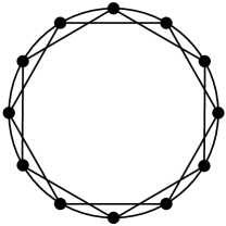
To study the synchronization in small-world networks, we consider the Newman-Watts model [11]. This model constructs a small-world network by starting from a K𝐾K-regular ring network (Fig. 1) as substrate, then randomly adds new links with probability p𝑝p.

Refer to caption
Figure 1: A 4-regular ring network.
Theorem 4.

Under assumptions 1 and 2, the limiting probability of stable synchronization of an unweighted Newman-Watts small-world network of oscillators, with parameters p𝑝p and K𝐾K, as N𝑁N\to\infty, is lower bounded by

PstabLB(ε|𝝀)=superscriptsubscript𝑃stabLBconditional𝜀𝝀absent\displaystyle P_{\mbox{\scriptsize stab}}^{\mbox{\scriptsize LB}}(\varepsilon|\mbox{$\boldsymbol{\lambda}$})= [i=2N1(ϕ1λiλ1ϕi)n]delimited-[]superscriptsubscriptproduct𝑖2𝑁1superscriptsubscriptitalic-ϕ1subscript𝜆𝑖subscript𝜆1subscriptitalic-ϕ𝑖𝑛\displaystyle\left[\prod_{i=2}^{N-1}\left(\frac{\phi_{1}~{}\lambda_{i}}{\lambda_{1}~{}\phi_{i}}\right)^{n}\right]
×j=0aj(N1)P((N1)n2+j,λ12ε2ϕ12σ2),\displaystyle\times\sum_{j=0}^{\infty}a^{(N-1)}_{j}P\left(\frac{(N-1)n}{2}+j,\frac{\lambda_{1}^{2}\varepsilon^{2}}{\phi_{1}^{2}\sigma^{2}}\right), (25)

where

σ=lim suptF𝜸𝚺𝜸F𝜸T+(K+Np)H𝜽𝚺𝜽H𝜽T1/2.𝜎subscriptlimit-supremum𝑡superscriptnormsubscriptF𝜸subscript𝚺𝜸superscriptsubscriptF𝜸𝑇𝐾𝑁𝑝subscriptH𝜽subscript𝚺𝜽subscriptsuperscriptH𝑇𝜽12\displaystyle\sigma=\limsup_{t\to\infty}~{}\|\mbox{{\bf F}}_{\mbox{$\boldsymbol{\gamma}$}}\mbox{$\boldsymbol{\Sigma}$}_{\mbox{$\boldsymbol{\gamma}$}}\mbox{{\bf F}}_{\mbox{$\boldsymbol{\gamma}$}}^{T}+(K+Np)\mbox{{\bf H}}_{\mbox{$\boldsymbol{\theta}$}}\mbox{$\boldsymbol{\Sigma}$}_{\mbox{$\boldsymbol{\theta}$}}\mbox{{\bf H}}^{T}_{\mbox{$\boldsymbol{\theta}$}}\|^{1/2}.
Proof.

The Laplacian matrix of a Newman-Watts small world network is

LNW=LRing+LER,subscriptLNWsubscriptLRingsubscriptLER\mbox{{\bf L}}_{\mbox{\scriptsize NW}}=\mbox{{\bf L}}_{\mbox{\scriptsize Ring}}+\mbox{{\bf L}}_{\mbox{\scriptsize ER}},

where LRingsubscriptLRing\mbox{{\bf L}}_{\mbox{\scriptsize Ring}} and LERsubscriptLER\mbox{{\bf L}}_{\mbox{\scriptsize ER}} are the laplacians of a K𝐾K-regular ring and an Erdös-Rényi network with parameter p𝑝p. Using Weyl’s inequalities we can bound the minimum and maximum eigenvalues of the small-world [21]

max{μminRing,μminER}μminNWdmin,subscriptsuperscript𝜇Ringsubscriptsuperscript𝜇ERsuperscriptsubscript𝜇NWsubscript𝑑\displaystyle\max\{\mu^{\mbox{\scriptsize Ring}}_{\min},\mu^{\mbox{\scriptsize ER}}_{\min}\}\leq\mu_{\min}^{\mbox{\scriptsize NW}}\leq d_{\min},
μmaxRing+μmaxERμmaxNWdmax,subscriptsuperscript𝜇Ringsubscriptsuperscript𝜇ERsuperscriptsubscript𝜇NWsubscript𝑑\displaystyle\mu^{\mbox{\scriptsize Ring}}_{\max}+\mu^{\mbox{\scriptsize ER}}_{\max}\geq\mu_{\max}^{\mbox{\scriptsize NW}}\geq d_{\max},

where the eigenvalues of a K𝐾K-regular ring is [21]

μiRingsubscriptsuperscript𝜇Ring𝑖\displaystyle\mu^{\mbox{\scriptsize Ring}}_{i} =\displaystyle= K2siniKπ2Ncos(K+2)iπ2NsiniπN,𝐾2𝑖𝐾𝜋2𝑁𝐾2𝑖𝜋2𝑁𝑖𝜋𝑁\displaystyle K-2\frac{\sin\frac{iK\pi}{2N}\cos\frac{(K+2)i\pi}{2N}}{\sin\frac{i\pi}{N}},

and subscripts min\min and max\max refer to smallest non-zero and maximum eigenvalue of L in corresponding configurations, respectively. The remaining of the proof is similar to that of Theorem 3 and is omitted in the interest of brevity. ∎

VII Numerical Example

In this section we verify our analytical results using numerical examples. We consider the van der Pol oscillator [20] which has the following dynamics

f(xi,𝜸i)=[xi2x1iγi(xi121)xi2].fsubscriptx𝑖subscript𝜸𝑖delimited-[]subscript𝑥𝑖2subscript𝑥1𝑖subscript𝛾𝑖subscriptsuperscript𝑥2𝑖11subscript𝑥𝑖2\displaystyle\mbox{{\bf f}}(\mbox{{\bf x}}_{i},\mbox{$\boldsymbol{\gamma}$}_{i})=\left[\begin{array}[]{c}x_{i2}\\ -x_{1i}-\gamma_{i}(x^{2}_{i1}-1)x_{i2}\end{array}\right]. (28)

We note that since the van der Pol oscillator has a limit cycle, as t𝑡t\to\infty, s is a periodic trajectory. Hence, the Jacobians are also periodic. We can, therefore, solve (6) analytically using Fourier series [20].

We assume that the nodes are coupled through their first states by

h(xj,xi,𝜽ij)=[θij1(x1jx1i)+θij20].hsubscriptx𝑗subscriptx𝑖subscript𝜽𝑖𝑗delimited-[]subscript𝜃𝑖𝑗1subscript𝑥1𝑗subscript𝑥1𝑖subscript𝜃𝑖𝑗20\mbox{{\bf h}}(\mbox{{\bf x}}_{j},\mbox{{\bf x}}_{i},\mbox{$\boldsymbol{\theta}$}_{ij})=\left[\begin{array}[]{c}\theta_{ij1}(x_{1j}-x_{1i})+\theta_{ij2}\\ 0\end{array}\right].

Thus, the Jacobians of f(.)\mbox{{\bf f}}(.)and h(.)\mbox{{\bf h}}(.) around (s,𝜸¯,𝜽¯)sbold-¯𝜸bold-¯𝜽(\mbox{{\bf s}},\mbox{$\boldsymbol{\bar{\gamma}}$},\mbox{$\boldsymbol{\bar{\theta}}$}) are

FxsubscriptFx\displaystyle\mbox{{\bf F}}_{\mbox{{\bf x}}} =\displaystyle= [0112γ¯s1s2γ¯(1s12)],delimited-[]0112¯𝛾subscript𝑠1subscript𝑠2¯𝛾1superscriptsubscript𝑠12\displaystyle\left[\begin{array}[]{cc}0&1\\ -1-2\bar{\gamma}s_{1}s_{2}&\bar{\gamma}(1-s_{1}^{2})\\ \end{array}\right],
HxsubscriptHx\displaystyle\mbox{{\bf H}}_{\mbox{{\bf x}}} =\displaystyle= [θ¯1000],delimited-[]subscript¯𝜃1000\displaystyle\left[\begin{array}[]{cc}\bar{\theta}_{1}&0\\ 0&0\\ \end{array}\right],
FγsubscriptF𝛾\displaystyle\mbox{{\bf F}}_{\gamma} =\displaystyle= [0(1s12)s2],delimited-[]01superscriptsubscript𝑠12subscript𝑠2\displaystyle\left[\begin{array}[]{c}0\\ (1-s_{1}^{2})s_{2}\\ \end{array}\right],
H𝜽subscriptH𝜽\displaystyle\mbox{{\bf H}}_{\mbox{$\boldsymbol{\theta}$}} =\displaystyle= [0100],delimited-[]0100\displaystyle\left[\begin{array}[]{cc}0&1\\ 0&0\\ \end{array}\right],

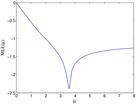
where s=[s1s2]Tssuperscriptdelimited-[]subscript𝑠1subscript𝑠2𝑇\mbox{{\bf s}}=[s_{1}~{}s_{2}]^{T}. Fig. 2 depicts the maximum Lyapunov exponent of FxμHxsubscriptFx𝜇subscriptHx\mbox{{\bf F}}_{\mbox{{\bf x}}}-\mu\mbox{{\bf H}}_{\mbox{{\bf x}}} as a function of μ𝜇\mu, where μ𝜇\mu is the eigenvalue of Laplacian matrix of the network.
Refer to caption
Figure 2: Maximum Lyapunov Exponent (MLE) as a function of eigenvalues of Laplacian matrix of the network, μ𝜇\mu.

Furthermore,

visubscriptv𝑖\displaystyle\mbox{{\bf v}}_{i} =[j=1Nujik=1Najkδθkj2(1s12)s2j=1Nujiδγj].absentdelimited-[]superscriptsubscript𝑗1𝑁superscriptsubscript𝑢𝑗𝑖superscriptsubscript𝑘1𝑁subscript𝑎𝑗𝑘𝛿subscript𝜃𝑘𝑗21superscriptsubscript𝑠12subscript𝑠2superscriptsubscript𝑗1𝑁superscriptsubscript𝑢𝑗𝑖𝛿subscript𝛾𝑗\displaystyle=\left[\begin{array}[]{c}\sum_{j=1}^{N}u_{ji}^{*}\sum_{k=1}^{N}a_{jk}\delta\theta_{kj2}\\ (1-s_{1}^{2})s_{2}\sum_{j=1}^{N}u_{ji}^{*}\delta\gamma_{j}\\ \end{array}\right]. (35)

It is clear that visubscriptv𝑖\mbox{{\bf v}}_{i} are independent of δθij1𝛿subscript𝜃𝑖𝑗1\delta\theta_{ij1}.

Refer to caption
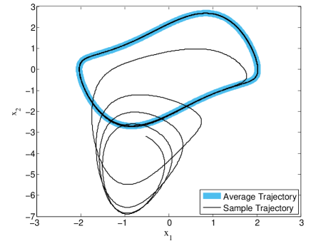
Figure 3: Synchronization manifold, s, and a sample trajectory, x1subscriptx1\mbox{{\bf x}}_{1}, for a ring network of van der Pol oscillators.

Also, covariance matrix of visubscriptv𝑖\mbox{{\bf v}}_{i} of a K𝐾K-regular ring network for 𝜸¯=1bold-¯𝜸1\mbox{$\boldsymbol{\bar{\gamma}}$}=1 can be calculated from (23) as

𝚺ii=[Kθ¯12σθ2200σγ2((1s12)s2)2],subscript𝚺𝑖𝑖delimited-[]𝐾superscriptsubscript¯𝜃12superscriptsubscript𝜎𝜃2200superscriptsubscript𝜎𝛾2superscript1superscriptsubscript𝑠12subscript𝑠22\displaystyle\mbox{$\boldsymbol{\Sigma}$}_{ii}=\left[\begin{array}[]{cc}K{\bar{\theta}}_{1}^{2}\sigma_{\theta 2}^{2}&0\\ 0&\sigma_{\gamma}^{2}((1-s_{1}^{2})s_{2})^{2}\end{array}\right], (38)

and

sup𝚺ii=[Kθ¯12σθ22009.93σγ2],supremumsubscript𝚺𝑖𝑖delimited-[]𝐾superscriptsubscript¯𝜃12superscriptsubscript𝜎𝜃22009.93superscriptsubscript𝜎𝛾2\displaystyle\sup\mbox{$\boldsymbol{\Sigma}$}_{ii}=\left[\begin{array}[]{cc}K\bar{\theta}_{1}^{2}\sigma_{\theta 2}^{2}&0\\ 0&9.93\sigma_{\gamma}^{2}\end{array}\right], (41)

where sup((1s12)s2)2supremumsuperscript1superscriptsubscript𝑠12subscript𝑠22\sup((1-s_{1}^{2})s_{2})^{2} is determined by simulation to be 9.939.939.93 and the supremums are calculated over one period of the limit cycle. Hence, σ=max(Kθ¯1σθ2,3.15σγ)𝜎𝐾subscript¯𝜃1subscript𝜎subscript𝜃23.15subscript𝜎𝛾\sigma=\max(\sqrt{K}\bar{\theta}_{1}\sigma_{\theta_{2}},3.15\sigma_{\gamma}).

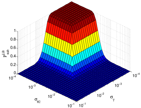
Now, consider a 666-regular ring network of size N=100𝑁100N=100, where γ𝒩(1,0.01)similar-to𝛾𝒩10.01\gamma\sim\mbox{${\mathcal{N}}$}(1,0.01) and 𝜽𝒩([10]T,0.01I)similar-to𝜽𝒩superscriptdelimited-[]10𝑇0.01I\mbox{$\boldsymbol{\theta}$}\sim\mbox{${\mathcal{N}}$}([1~{}0]^{T},0.01\mbox{{\bf I}}). Fig. 3 depicts the synchronization manifold, s, and a sample trajectory, x1subscriptx1\mbox{{\bf x}}_{1}, converging to s. Fig. 4 presents the analytical lower bound on the probability of stable ε𝜀\varepsilon-synchronization in the considered ring network, as a function of σθ2subscript𝜎subscript𝜃2\sigma_{\theta_{2}} and σγsubscript𝜎𝛾\sigma_{\gamma} for ε=0.40𝜀0.40\varepsilon=0.40. As it can be seen, the probability of synchronization falls sharply as the variances of mismatches increase. Moreover, we observe that the range of σγsubscript𝜎𝛾\sigma_{\gamma} and σθ2subscript𝜎subscript𝜃2\sigma_{\theta_{2}} for which the network is stable with high probability is rectangular. This is explained by noting that σ𝜎\sigma is related to the maximum of σγsubscript𝜎𝛾\sigma_{\gamma} and σθ2subscript𝜎subscript𝜃2\sigma_{\theta_{2}}, as it can be seen in (41). Another observation from Fig. 4 is that even small mismatches leads to instability of the synchronization state even with a relatively large tolerance of ε=0.40𝜀0.40\varepsilon=0.40.

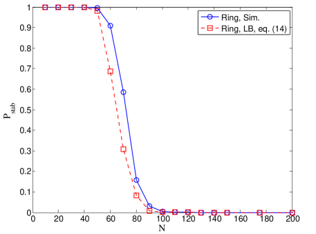
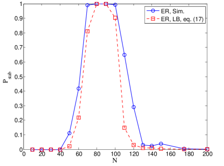
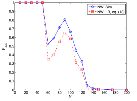
We now proceed to compare a ring network, an Erdös-Rényi network and a Newman-Watts (small-world) network. For a fair comparison, we choose the network parameters such that all networks have the same number of nodes and the same average node degree. That is, we consider a N=100𝑁100N=100 node, 101010-regular ring, an Erdös-Rényi network with N=100𝑁100N=100 and randomness parameter p=0.1𝑝0.1p=0.1, and a Newman-Watts network generated from a N=100𝑁100N=100 node, 666-regular ring and link addition probability p=0.4×100/94=0.4167𝑝0.4100940.4167p=0.4\times 100/94=0.4167. Fig. 5 presents the probability of stability versus network size, N𝑁N, for these three networks with ε=0.4𝜀0.4\varepsilon=0.4. As it can be seen for the Ring network (Fig. 5 (a)), as N𝑁N increases, even though the variance of the mismatch input is constant, σ=3.15σγ𝜎3.15subscript𝜎𝛾\sigma=3.15\sigma_{\gamma}, the ε𝜀\varepsilon-synchronization of the network deteriorates. This is because as the degree of the nodes are kept constant and network size increases, the algebraic connectivity111Algebraic connectivity is defined as the second smallest eigenvalue of the Laplacian matrix of a network.[21]. of the network,

μN1ring=k2sin(kπ/2N)cos((k+2)π/2N)sin(π/N),subscriptsuperscript𝜇ring𝑁1𝑘2𝑘𝜋2𝑁𝑘2𝜋2𝑁𝜋𝑁\mu^{\scriptsize\mbox{ring}}_{N-1}=k-2\frac{\sin(k\pi/2N)\cos((k+2)\pi/2N)}{\sin(\pi/N)},

decreases. For large N𝑁N, in our example, smaller algebraic connectivity means smaller MLE (See Fig. 2), hence the probability of ε𝜀\varepsilon-synchronization falls sharply.

Refer to caption
Figure 4: PstabLBsubscriptsuperscript𝑃LBstabP^{\mbox{\scriptsize LB}}_{\mbox{\scriptsize stab}} in the ring network as a function of σθ2subscript𝜎subscript𝜃2\sigma_{\theta_{2}} and σγsubscript𝜎𝛾\sigma_{\gamma} for ε=0.4𝜀0.4\varepsilon=0.4.

Fig. 5 (b) presents the probability of ε𝜀\varepsilon-stability of the Erdös-Rényi network. It is interesting to note that since the network is disconnected for smaller network sizes, the network is not synchronized. As network size continues to grow, the network becomes connected and synchronization behavior emerges. This behavior continues until the growth in the network size, increases the variance of the mismatch input, v, to the extent that the network falls out of ε𝜀\varepsilon-stability.

Fig. 5 (c) presents the probability of ε𝜀\varepsilon-stability for the Newman-Watts network. It is interesting to note the mechanisms at work as N𝑁N increases: At first, when N𝑁N is small there are very few added links given a small value of p𝑝p. Thus, the network has not yet transitioned into a small-world and its algebraic connectivity is still quite close to that of the ring topology. Thus, as the size of the network increases its second smallest eigenvalue decreases. Since the variance of mismatch, v, is constant (σb=3.15σγsubscript𝜎𝑏3.15subscript𝜎𝛾\sigma_{b}=3.15\sigma_{\gamma}), the probability of stability decreases. As N𝑁N continues to increase, by adding links in random, sufficient number of long range connections are established and the small-world transition is achieved. Consequently, algebraic connectivity of the network starts to grow rapidly. Hence, λisubscript𝜆𝑖\lambda_{i} increase and, therefore, PstabLBsubscriptsuperscript𝑃LBstabP^{\mbox{\scriptsize LB}}_{\mbox{\scriptsize stab}} improves. As N𝑁N continues to increases K+Npσθ2𝐾𝑁𝑝subscript𝜎subscript𝜃2\sqrt{K+Np}\sigma_{\theta_{2}} overtakes 3.15σγ3.15subscript𝜎𝛾3.15\sigma_{\gamma} in the variance of mismatch and its destructive effect surpasses the improvement caused by transition to small-world. Consequently, we observe that PstabLBsubscriptsuperscript𝑃LBstabP^{\mbox{\scriptsize LB}}_{\mbox{\scriptsize stab}} begins to drop.

Refer to caption
(a)
Refer to caption
(b)
Refer to caption
(c)
Figure 5: Probability of stability as a function N𝑁N, for (a) ring, (b) Erdös-Rényi, and (c) Newman-Watts networks.
Refer to caption
(a)
Refer to caption
(b)
Refer to caption
(c)
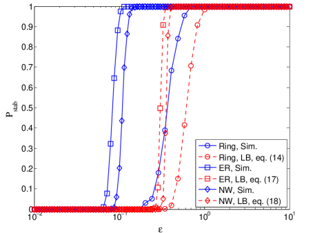
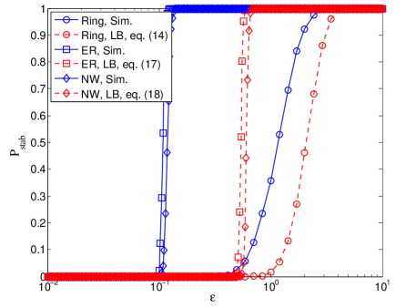
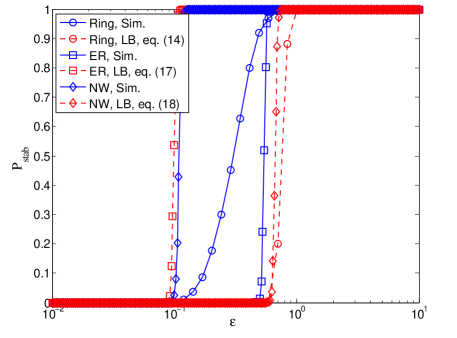
Figure 6: Pstabsubscript𝑃stabP_{\mbox{\scriptsize stab}} as a function of ε𝜀\varepsilon for the ring, NW and Erdös-Rényi networks: (a) N=100,d¯=10formulae-sequence𝑁100¯𝑑10N=100,\bar{d}=10, (b) N=200,d¯=10formulae-sequence𝑁200¯𝑑10N=200,\bar{d}=10, and N=200,d¯=20formulae-sequence𝑁200¯𝑑20N=200,\bar{d}=20.

Figs. 6 (a) through (c) depict the probability of ε𝜀\varepsilon-stability as a function of ε𝜀\varepsilon in the considered Ring, Erdös-Réyni, and Newman-Watts networks for different N𝑁N and d¯¯𝑑\bar{d}: (a) N=100,d¯=10formulae-sequence𝑁100¯𝑑10N=100,\bar{d}=10, (b) N=200,d¯=10formulae-sequence𝑁200¯𝑑10N=200,\bar{d}=10, and N=200,d¯=20formulae-sequence𝑁200¯𝑑20N=200,\bar{d}=20. As it can be seen, the analytical lower bound and the simulation result for the ring network are reasonably close. This is due to the homogeneity of its node degrees, i.e. di=Ksubscript𝑑𝑖𝐾d_{i}=K, which holds true for the other networks as N𝑁N approaches infinity. The other point directly observed from these figures is that the rise in the probability of the stability is much sharper in the Erdös-Réyni and Newman-Watts networks, this is because the spread of the spectrum, [μmin,μmaxsubscript𝜇subscript𝜇\mu_{\min},\mu_{\max}], for these networks are smaller than that of ring topology. This, in fact, causes the Lyapunov exponents of the traverse modes to be closer to each other and hence the networks become easily and rapidly synchronized. Other interesting observation is that the results for the Erdös-Réyni and Newman-Watts networks are similar. The reason can be sought in the effectiveness of communication in both networks to each other. As it has been shown in [10], even though small-worlds are strongly locally connected (due to ring substrate), they have almost the same average shortest path length of Erdös-Réyni networks. This results in almost the same communication efficiency in small-worlds as Erdös-Réyni network. Hence, the synchronizability of both types of networks are similar.

VIII Conclusion

We had seen that mismatch in either couplings or the local dynamics does not allow perfect synchronization. Rather, the network can only be synchronized to a neighborhood of the synchronization manifold. Considering this relaxed notion of synchronization we have provided a generalized master stability function that takes the mismatches into account. We then used this master stability function to derive lower bounds on the probability of synchronization in regular, Erdös-Rényi, and Newman-Watts networks. We verified our results using numerical examples involving networks of van der Pol oscillators. These examples clearly shows the different phase transition behavior of the different network models.

Appendix A Proof of Lemma 2

Proof.

The state space equation for the 𝜼isubscript𝜼𝑖\mbox{$\boldsymbol{\eta}$}_{i} can be written as

𝜼i˙˙subscript𝜼𝑖\displaystyle\dot{\mbox{$\boldsymbol{\eta}$}_{i}} =\displaystyle= (FxμHx)𝜼i+(FxHx)𝜼i+1+vi(t),subscriptFx𝜇subscriptHxsubscript𝜼𝑖subscriptFxsubscriptHxsubscript𝜼𝑖1subscriptv𝑖𝑡\displaystyle\left(\mbox{{\bf F}}_{\mbox{{\bf x}}}-\mu\mbox{{\bf H}}_{\mbox{{\bf x}}}\right)\mbox{$\boldsymbol{\eta}$}_{i}+(\mbox{{\bf F}}_{\mbox{{\bf x}}}-\mbox{{\bf H}}_{\mbox{{\bf x}}})\mbox{$\boldsymbol{\eta}$}_{i+1}+\mbox{{\bf v}}_{i}(t), (42)

for iN𝑖𝑁i\neq N, and

𝜼N˙˙subscript𝜼𝑁\displaystyle\dot{\mbox{$\boldsymbol{\eta}$}_{N}} =\displaystyle= (FxμHx)𝜼N+vN(t).subscriptFx𝜇subscriptHxsubscript𝜼𝑁subscriptv𝑁𝑡\displaystyle\left(\mbox{{\bf F}}_{\mbox{{\bf x}}}-\mu\mbox{{\bf H}}_{\mbox{{\bf x}}}\right)\mbox{$\boldsymbol{\eta}$}_{N}+\mbox{{\bf v}}_{N}(t). (43)

The solution of (42) and (43) are

𝜼i(t)subscript𝜼𝑖𝑡\displaystyle\mbox{$\boldsymbol{\eta}$}_{i}(t) =\displaystyle= 𝚽(t,0)𝜼i(0)+0t𝚽(t,τ)vi(τ)𝑑τ𝚽𝑡0subscript𝜼𝑖0superscriptsubscript0𝑡𝚽𝑡𝜏subscriptv𝑖𝜏differential-d𝜏\displaystyle\mathbf{\Phi}(t,0)\mbox{$\boldsymbol{\eta}$}_{i}(0)+\int_{0}^{t}\mathbf{\Phi}(t,\tau)\mbox{{\bf v}}_{i}(\tau)d\tau
+0t𝚽(t,τ)(FxHx)𝜼i+1(τ)𝑑τ,superscriptsubscript0𝑡𝚽𝑡𝜏subscriptFxsubscriptHxsubscript𝜼𝑖1𝜏differential-d𝜏\displaystyle+\int_{0}^{t}\mathbf{\Phi}(t,\tau)(\mbox{{\bf F}}_{\mbox{{\bf x}}}-\mbox{{\bf H}}_{\mbox{{\bf x}}})\mbox{$\boldsymbol{\eta}$}_{i+1}(\tau)d\tau,

for iN𝑖𝑁i\neq N and

𝜼N(t)subscript𝜼𝑁𝑡\displaystyle\mbox{$\boldsymbol{\eta}$}_{N}(t) =\displaystyle= 𝚽(t,0)𝜼N(0)+0t𝚽(t,τ)vN(τ)𝑑τ,𝚽𝑡0subscript𝜼𝑁0superscriptsubscript0𝑡𝚽𝑡𝜏subscriptv𝑁𝜏differential-d𝜏\displaystyle\mathbf{\Phi}(t,0)\mbox{$\boldsymbol{\eta}$}_{N}(0)+\int_{0}^{t}\mathbf{\Phi}(t,\tau)\mbox{{\bf v}}_{N}(\tau)d\tau,

where 𝚽(t,τ)=𝐙(t)𝐙1(τ)𝚽𝑡𝜏𝐙𝑡superscript𝐙1𝜏\mathbf{\Phi}(t,\tau)=\mathbf{Z}(t)\mathbf{Z}^{-1}(\tau), and 𝐙𝐙\mathbf{Z} is the normal fundamental matrix of FxμHxsubscriptFx𝜇subscriptHx\mbox{{\bf F}}_{\mbox{{\bf x}}}-\mu\mbox{{\bf H}}_{\mbox{{\bf x}}} [23].

Applying triangle inequality yields

𝜼i(t)delimited-∥∥subscript𝜼𝑖𝑡\displaystyle\lVert\mbox{$\boldsymbol{\eta}$}_{i}(t)\rVert \displaystyle\leq 𝚽(t,0)𝜼i(0)delimited-∥∥𝚽𝑡0delimited-∥∥subscript𝜼𝑖0\displaystyle\lVert\mathbf{\Phi}(t,0)\rVert\lVert\mbox{$\boldsymbol{\eta}$}_{i}(0)\rVert
+0t(FxHx)𝜼i+1(τ)+vi(τ)𝚽(t,τ)𝑑τ,superscriptsubscript0𝑡delimited-∥∥subscriptFxsubscriptHxsubscript𝜼𝑖1𝜏subscriptv𝑖𝜏delimited-∥∥𝚽𝑡𝜏differential-d𝜏\displaystyle+\int_{0}^{t}\lVert(\mbox{{\bf F}}_{\mbox{{\bf x}}}-\mbox{{\bf H}}_{\mbox{{\bf x}}})\mbox{$\boldsymbol{\eta}$}_{i+1}(\tau)+\mbox{{\bf v}}_{i}(\tau)\rVert\lVert\mathbf{\Phi}(t,\tau)\rVert d\tau,

for i{1,,N1}𝑖1𝑁1i\in\{1,...,N-1\}, and

𝜼N(t)delimited-∥∥subscript𝜼𝑁𝑡\displaystyle\lVert\mbox{$\boldsymbol{\eta}$}_{N}(t)\rVert \displaystyle\leq 𝚽(t,0)𝜼N(0)+0tvN(τ)𝚽(t,τ)𝑑τ,delimited-∥∥𝚽𝑡0delimited-∥∥subscript𝜼𝑁0superscriptsubscript0𝑡delimited-∥∥subscriptv𝑁𝜏delimited-∥∥𝚽𝑡𝜏differential-d𝜏\displaystyle\lVert\mathbf{\Phi}(t,0)\rVert\lVert\mbox{$\boldsymbol{\eta}$}_{N}(0)\rVert+\int_{0}^{t}\lVert\mbox{{\bf v}}_{N}(\tau)\rVert\lVert\mathbf{\Phi}(t,\tau)\rVert d\tau,

which, as t𝑡t\to\infty, yields

lim supt𝜼isubscriptlimit-supremum𝑡delimited-∥∥subscript𝜼𝑖\displaystyle\limsup_{t\to\infty}\lVert\mbox{$\boldsymbol{\eta}$}_{i}\rVert \displaystyle\leq 𝜼i(0)lim supt𝚽(t,0)delimited-∥∥subscript𝜼𝑖0subscriptlimit-supremum𝑡delimited-∥∥𝚽𝑡0\displaystyle\lVert\mbox{$\boldsymbol{\eta}$}_{i}(0)\rVert\limsup_{t\to\infty}\lVert\mathbf{\Phi}(t,0)\rVert (44)
+lim suptvilim supt0t𝚽(t,τ))dτ\displaystyle+\limsup_{t\to\infty}\lVert\mbox{{\bf v}}_{i}\rVert\limsup_{t\to\infty}\int_{0}^{t}\lVert\mathbf{\Phi}(t,\tau))\rVert d\tau
+lim suptFxHxlim supt𝜼i+1subscriptlimit-supremum𝑡delimited-∥∥subscriptFxsubscriptHxsubscriptlimit-supremum𝑡delimited-∥∥subscript𝜼𝑖1\displaystyle+\limsup_{t\to\infty}\lVert\mbox{{\bf F}}_{\mbox{{\bf x}}}-\mbox{{\bf H}}_{\mbox{{\bf x}}}\rVert\limsup_{t\to\infty}\lVert\mbox{$\boldsymbol{\eta}$}_{i+1}\rVert
×lim supt0t𝚽(t,τ)dτ,\displaystyle\quad\quad\quad\quad\times\limsup_{t\to\infty}\int_{0}^{t}\lVert\mathbf{\Phi}(t,\tau)\rVert d\tau,

and

lim supt𝜼Nsubscriptlimit-supremum𝑡delimited-∥∥subscript𝜼𝑁absent\displaystyle\limsup_{t\to\infty}\lVert\mbox{$\boldsymbol{\eta}$}_{N}\rVert\leq 𝜼N(0)lim supt𝚽(t,0)delimited-∥∥subscript𝜼𝑁0subscriptlimit-supremum𝑡delimited-∥∥𝚽𝑡0\displaystyle\lVert\mbox{$\boldsymbol{\eta}$}_{N}(0)\rVert\limsup_{t\to\infty}\lVert\mathbf{\Phi}(t,0)\rVert
+lim suptvNlim supt0t𝚽(t,τ)𝑑τ.subscriptlimit-supremum𝑡delimited-∥∥subscriptv𝑁subscriptlimit-supremum𝑡superscriptsubscript0𝑡delimited-∥∥𝚽𝑡𝜏differential-d𝜏\displaystyle+\limsup_{t\to\infty}\lVert\mbox{{\bf v}}_{N}\rVert\limsup_{t\to\infty}\int_{0}^{t}\lVert\mathbf{\Phi}(t,\tau)\rVert d\tau. (45)

We know that there exists positive real ϕitalic-ϕ\phi such that [23]

𝚽(t,τ)ϕeλ(tτ),delimited-∥∥𝚽𝑡𝜏italic-ϕsuperscript𝑒𝜆𝑡𝜏\displaystyle\lVert\mathbf{\Phi}(t,\tau)\rVert\leq\phi e^{-\lambda(t-\tau)},

where λ𝜆\lambda is the maximum Lyapunov exponent of FxμHxsubscriptFx𝜇subscriptHx\mbox{{\bf F}}_{\mbox{{\bf x}}}-\mu\mbox{{\bf H}}_{\mbox{{\bf x}}}. If λ>0𝜆0\lambda>0 this yields

lim supt𝚽(t,0))\displaystyle\limsup_{t\to\infty}\lVert\mathbf{\Phi}(t,0))\rVert =\displaystyle= 0,0\displaystyle 0,
lim supt0t𝚽(t,τ))dτ\displaystyle\limsup_{t\to\infty}\int_{0}^{t}\lVert\mathbf{\Phi}(t,\tau))\rVert d\tau \displaystyle\leq ϕλ.italic-ϕ𝜆\displaystyle\frac{\phi}{\lambda}.

Substituting in (44) and (45) yields,

lim supt𝜼isubscriptlimit-supremum𝑡delimited-∥∥subscript𝜼𝑖\displaystyle\limsup_{t\to\infty}\lVert\mbox{$\boldsymbol{\eta}$}_{i}\rVert \displaystyle\leq ϕλlim suptFxHx𝜼i+1italic-ϕ𝜆subscriptlimit-supremum𝑡delimited-∥∥subscriptFxsubscriptHxdelimited-∥∥subscript𝜼𝑖1\displaystyle\frac{\phi}{\lambda}\limsup_{t\to\infty}\lVert\mbox{{\bf F}}_{\mbox{{\bf x}}}-\mbox{{\bf H}}_{\mbox{{\bf x}}}\rVert\lVert\mbox{$\boldsymbol{\eta}$}_{i+1}\rVert
+ϕλlim suptvi,italic-ϕ𝜆subscriptlimit-supremum𝑡delimited-∥∥subscriptv𝑖\displaystyle+\frac{\phi}{\lambda}\limsup_{t\to\infty}\lVert\mbox{{\bf v}}_{i}\rVert,

and

lim supt𝜼Nsubscriptlimit-supremum𝑡delimited-∥∥subscript𝜼𝑁\displaystyle\limsup_{t\to\infty}\lVert\mbox{$\boldsymbol{\eta}$}_{N}\rVert \displaystyle\leq ϕλlim suptvN.italic-ϕ𝜆subscriptlimit-supremum𝑡delimited-∥∥subscriptv𝑁\displaystyle\frac{\phi}{\lambda}\limsup_{t\to\infty}\lVert\mbox{{\bf v}}_{N}\rVert.

Solving the recursive inequalities we get

lim supt𝜼isubscriptlimit-supremum𝑡delimited-∥∥subscript𝜼𝑖\displaystyle\limsup_{t\to\infty}\lVert\mbox{$\boldsymbol{\eta}$}_{i}\rVert \displaystyle\leq j=iN(ϕλ)Nj+1lim suptFx+HxNjsuperscriptsubscript𝑗𝑖𝑁superscriptitalic-ϕ𝜆𝑁𝑗1subscriptlimit-supremum𝑡superscriptdelimited-∥∥subscriptFxsubscriptHx𝑁𝑗\displaystyle\sum_{j=i}^{N}\left(\frac{\phi}{\lambda}\right)^{N-j+1}\limsup_{t\to\infty}\lVert\mbox{{\bf F}}_{\mbox{{\bf x}}}+\mbox{{\bf H}}_{\mbox{{\bf x}}}\rVert^{N-j}
×lim suptvj.\displaystyle\quad\quad\quad\quad\times\limsup_{t\to\infty}\lVert\mbox{{\bf v}}_{j}\rVert.

Appendix B Covariance of v

The covariance of v is

𝚺v=E[(vv¯)(vv¯)T]=[𝚺ij],subscript𝚺v𝐸delimited-[]v¯vsuperscriptv¯v𝑇delimited-[]subscript𝚺𝑖𝑗\displaystyle\mbox{$\boldsymbol{\Sigma}$}_{\mbox{{\bf v}}}={E}[(\mbox{{\bf v}}-\bar{\mbox{{\bf v}}})(\mbox{{\bf v}}-\bar{\mbox{{\bf v}}})^{T}]=[\mbox{$\boldsymbol{\Sigma}$}_{ij}],

where v¯=h(s,s,𝜽¯)(Dind¯inI)¯vtensor-producthss¯𝜽superscriptDinsubscript¯𝑑inI\bar{\mbox{{\bf v}}}=\mbox{{\bf h}}(\mbox{{\bf s}},\mbox{{\bf s}},\bar{\mbox{$\boldsymbol{\theta}$}})\otimes(\mbox{{\bf D}}^{\scriptsize\mbox{in}}-\bar{d}_{\scriptsize\mbox{in}}\mbox{{\bf I}}) and Din=diag([d1indNin])superscriptDindiagdelimited-[]superscriptsubscript𝑑1insuperscriptsubscript𝑑𝑁in\mbox{{\bf D}}^{\scriptsize\mbox{in}}=\mbox{diag}([d_{1}^{\scriptsize\mbox{in}}\cdots d_{N}^{\scriptsize\mbox{in}}]). Thus, the ij𝑖𝑗ijth block of 𝚺vsubscript𝚺v\mbox{$\boldsymbol{\Sigma}$}_{\mbox{{\bf v}}} is

𝚺ijsubscript𝚺𝑖𝑗\displaystyle\mbox{$\boldsymbol{\Sigma}$}_{ij} =\displaystyle= k,l𝒩uikujlE[(F𝜸δ𝜸k+m𝒩amkH𝜽δ𝜽mk)\displaystyle\sum_{k,l\in\mbox{${\mathcal{N}}$}}u_{ik}u_{jl}^{\star}E\left[\left(\mbox{{\bf F}}_{\mbox{$\boldsymbol{\gamma}$}}\delta\mbox{$\boldsymbol{\gamma}$}_{k}+\sum_{m\in\mbox{${\mathcal{N}}$}}a_{mk}\mbox{{\bf H}}_{\mbox{$\boldsymbol{\theta}$}}\delta\mbox{$\boldsymbol{\theta}$}_{mk}\right)\right.
×(F𝜸δ𝜸l+n𝒩alnH𝜽δ𝜽nl)T]\displaystyle\times\left.\left(\mbox{{\bf F}}_{\mbox{$\boldsymbol{\gamma}$}}\delta\mbox{$\boldsymbol{\gamma}$}_{l}+\sum_{n\in\mbox{${\mathcal{N}}$}}a_{ln}\mbox{{\bf H}}_{\mbox{$\boldsymbol{\theta}$}}\delta\mbox{$\boldsymbol{\theta}$}_{nl}\right)^{T}\right]
=\displaystyle= k,l𝒩uikujlF𝜸𝚺𝜸F𝜸Tsubscript𝑘𝑙𝒩subscript𝑢𝑖𝑘superscriptsubscript𝑢𝑗𝑙subscriptF𝜸subscript𝚺𝜸superscriptsubscriptF𝜸𝑇\displaystyle\sum_{k,l\in\mbox{${\mathcal{N}}$}}u_{ik}u_{jl}^{\star}\mbox{{\bf F}}_{\mbox{$\boldsymbol{\gamma}$}}\mbox{$\boldsymbol{\Sigma}$}_{\mbox{$\boldsymbol{\gamma}$}}\mbox{{\bf F}}_{\mbox{$\boldsymbol{\gamma}$}}^{T}
+k,l,m,n𝒩uikujlakmalnH𝜽𝚺𝜽H𝜽T𝟙k=l𝟙m=nsubscript𝑘𝑙𝑚𝑛𝒩subscript𝑢𝑖𝑘superscriptsubscript𝑢𝑗𝑙subscript𝑎𝑘𝑚subscript𝑎𝑙𝑛subscriptH𝜽subscript𝚺𝜽superscriptsubscriptH𝜽𝑇subscript1𝑘𝑙subscript1𝑚𝑛\displaystyle+\sum_{k,l,m,n\in\mbox{${\mathcal{N}}$}}u_{ik}u_{jl}^{\star}a_{km}a_{ln}\mbox{{\bf H}}_{\mbox{$\boldsymbol{\theta}$}}\mbox{$\boldsymbol{\Sigma}$}_{\mbox{$\boldsymbol{\theta}$}}\mbox{{\bf H}}_{\mbox{$\boldsymbol{\theta}$}}^{T}\mathbbm{1}_{k=l}\mathbbm{1}_{m=n}
=\displaystyle= F𝜸𝚺𝜸F𝜸T1i=j+k,m𝒩uikujk|akm|2H𝜽𝚺𝜽H𝜽T.subscriptF𝜸subscript𝚺𝜸superscriptsubscriptF𝜸𝑇subscript1𝑖𝑗subscript𝑘𝑚𝒩subscript𝑢𝑖𝑘superscriptsubscript𝑢𝑗𝑘superscriptsubscript𝑎𝑘𝑚2subscriptH𝜽subscript𝚺𝜽superscriptsubscriptH𝜽𝑇\displaystyle\mbox{{\bf F}}_{\mbox{$\boldsymbol{\gamma}$}}\mbox{$\boldsymbol{\Sigma}$}_{\mbox{$\boldsymbol{\gamma}$}}\mbox{{\bf F}}_{\mbox{$\boldsymbol{\gamma}$}}^{T}1_{i=j}+\sum_{k,m\in\mbox{${\mathcal{N}}$}}u_{ik}u_{jk}^{\star}\lvert a_{km}\rvert^{2}\mbox{{\bf H}}_{\mbox{$\boldsymbol{\theta}$}}\mbox{$\boldsymbol{\Sigma}$}_{\mbox{$\boldsymbol{\theta}$}}\mbox{{\bf H}}_{\mbox{$\boldsymbol{\theta}$}}^{T}.

References

  • [1] N. Wiener, Cybernetics or Control and Communication in the Animal and the Machine.   MIT press, 1965, vol. 25.
  • [2] A. Arenas, A. Díaz-Guilera, J. Kurths, Y. Moreno, and C. Zhou, “Synchronization in complex networks,” Physics Reports, vol. 469, no. 3, pp. 93–153, 2008.
  • [3] A. T. Winfree, “Biological rhythms and the behavior of populations of coupled oscillators,” Journal of Theoretical Biology, vol. 16, no. 1, pp. 15 – 42, 1967.
  • [4] M. E. J. Newman, Networks: An Introduction.   Oxford University Press, 2010.
  • [5] L. M. Pecora and T. L. Carroll, “Master stability for synchronized coupled system,” Physical Review Letters, vol. 80, no. 10, pp. 2109–2112, 1998.
  • [6] A. E. Motter, “Bounding network spectra for network design,” New Journal of Physics, vol. 9, no. 6, p. 182, 2007. [Online]. Available: http://stacks.iop.org/1367-2630/9/i=6/a=182
  • [7] Z. F. Wang and G. Chen, “Synchronization in small-world dynamical networks,” International Journal of Bifurcation and Chaos, vol. 12, pp. 187–192, 2002.
  • [8] S. Manaffam and A. Seyedi, “Synchronization probability in large complex networks,” IEEE Transactions on Circuits and Systems II, vol. 60, no. 10, pp. 697–701, Oct. 2013.
  • [9] C. Zhou, A. E. Motter, and J. Kurths, “Universality in the synchronization of weighted random networks,” Phys. Rev. Lett., vol. 96, no. 3, p. 034101, Jan 2006.
  • [10] D. J. Watts and S. H. Strogatz, “Collective dynamics of ‘Small-World’ networks,” Letters to Nature, vol. 393, pp. 440–442, 1998.
  • [11] M. E. J. Newman and D. Watts, “Scaling and percolation in the small world network model,” Physics Letter E, vol. 60, pp. 7332–7342, 1999.
  • [12] Y. Wu, Y. Shang, M. Chen, C. Zhou, and J. Kurths, “Synchronization in small-world networks,” Chaos, vol. 18, no. 3, pp. 157–165, September 2008.
  • [13] T. Nishikawa, A. E. Motter, Y.-C. Lai, and F. C. Hoppensteadt, “Heterogeneity in oscillator networks: Are smaller worlds easier to synchronize?” Phys. Rev. Lett., vol. 91, no. 1, p. 014101, Jul 2003.
  • [14] J. G. Restrepo, E. Ott, and B. R. Hunt, “Spatial patterns of desynchronization bursts in networks,” Phys. Rev. E, vol. 69, no. 6, p. 066215, Jun 2004.
  • [15] J. Sun, E. M. Bolit, and T. Nishikawa, “Master stability functions for coupled nearly identical dynamical systems,” Europhysics Letters, vol. 85, no. 6, pp. 1–5, 2009.
  • [16] F. Sorrentino and M. Porfiri, “Synchronization of coupled nonidentical dynamical systems,” Europhysics Letters, vol. 93, no. 5, pp. 1–7, 2011.
  • [17] J. Xiang and G. Chen, “On the v-stability of complex dynamical networks,” Automatica, vol. 43, no. 6, pp. 1049 – 1057, 2007.
  • [18] J. Zhao, D. J. Hill, and T. Liu, “Global bounded synchronization of general dynamical networks with nonidentical nodes,” Transactions on Automatic Control, vol. 57, no. 10, pp. 2656–2572, October 2012.
  • [19] S. Acharyya and R. E. Amritkar, “Analysis of parameter mismatches in the master stability function for network synchronization,” Letters Journal Exploring the Frontiers of Physics, vol. 99, no. 4, pp. 1–7, 20121.
  • [20] D. Poland, “Loci of limit cycles,” Physical Review E, vol. 49, no. 1, pp. 49–57, January 1994.
  • [21] B. Mohar, The Laplacian spectrum of graphs.   Wiley, 1991.
  • [22] P. Moschopoulos and W. Canada, “The distribution function of a linear combination of chi-squares,” Computers and Mathematics with Applications, vol. 10, no. 4–5, pp. 383 – 386, 1984.
  • [23] J. L. Daleckii and M. G. Krein, Stability of Solutions of Differential Equations in Banach Space.   American Mathematical Society, 1974, vol. 43.