The equation of state in (2+1)-flavor QCD

Abstract

We present results for the equation of state in (2+1)-flavor QCD using the highly improved staggered quark action and lattices with temporal extent $N_{\tau}=6,\leavevmode\nobreak\ 8,\leavevmode\nobreak\ 10$, and $12$. We show that these data can be reliably extrapolated to the continuum limit and obtain a number of thermodynamic quantities and the speed of sound in the temperature range (130–400) MeV. We compare our results with previous calculations, and provide an analytic parameterization of the pressure, from which other thermodynamic quantities can be calculated, for use in phenomenology. We show that the energy density in the crossover region, $145\leavevmode\nobreak\ {\rm MeV}\leq T\leq 163$ MeV, defined by the chiral transition, is $\epsilon_{c}=(0.18-0.5)\leavevmode\nobreak\ {\rm GeV}/{\rm fm}^{3}$, $i.e.$, $(1.2-3.1)\ \epsilon_{\rm nuclear}$. At high temperatures, we compare our results with resummed and dimensionally reduced perturbation theory calculations. As a byproduct of our analyses, we obtain the values of the scale parameters $r_{0}$ from the static quark potential and $w_{0}$ from the gradient flow.

March 18, 2024

I Introduction

At high temperatures, matter governed by strong interactions (strong interaction matter) undergoes a deconfining transition to a new state, in which the thermodynamics can be described in terms of quark and gluon degrees of freedom. The equation of state (EoS) of such matter, just as for many other thermodynamic systems, is of fundamental importance for understanding its composition as well as its static and dynamical properties. Studying the properties of this matter using Quantum Chromo-Dynamics (QCD) was made possible by the formulation of lattice-regularized QCD Wilson (1974) and the development of numerical algorithms for its analysis Creutz (1980). Lattice calculations of the QCD EoS were first performed in 1980 Engels et al. (1981), and, driven by the steady growth in computing resources and the development of new simulation algorithms, there now exist precise results for the transition temperature Aoki et al. (2009); Bazavov et al. (2012a), fluctuations of conserved charges Borsanyi et al. (2012a); Bazavov et al. (2012b, 2014) as well as the EoS. For recent reviews see for instance Refs. Petreczky (2012a); Philipsen (2013); DeTar and Heller (2009).

The EoS contains information on the relevant degrees of freedom in the thermal medium in different temperature regimes and reflects the transition between different states of matter. A quantitative description of the QCD EoS over a wide temperature range is needed to understand the expansion and cooling of matter in the early universe, as well as of the hot dense nuclear matter created in heavy ion collisions.

To study the QCD EoS across a transition between different states of matter, at which the internal degrees of freedom are highly correlated, requires nonperturbative techniques. However, in the case of strong interaction matter, the need for nonperturbative methods is not restricted to the strongly interacting region close to the QCD transition temperature, but is also needed far above this deconfining transition where well-known infrared problems Linde (1980) prohibit a straightforward perturbative analysis of QCD thermodynamics. Also, at low temperatures, where the hadron resonance gas models (HRG) for the description of the hadronic equation of state are quite successful Braun-Munzinger et al. (2003), lattice QCD calculations are important as they provide the benchmark estimates of thermal properties of in-medium hadrons and the EoS of hadronic matter. In summary, simulations of lattice QCD provide the best approach over the full phenomenologically interesting temperature range in which all sources of errors can be quantified and systematically improved.

The deconfining transition in QCD, with small but non-zero values of the light quark masses, is a rapid crossover that coincides with the restoration of chiral symmetry Aoki et al. (2009); Bazavov et al. (2012a). In fact, it is the latter that characterizes the second order phase transition that occurs in the chiral limit of QCD at finite temperature. At this phase transition the spontaneously broken chiral symmetry is restored. The universal scaling properties of this chiral transition are used to determine the pseudo-critical temperature $T_{c}$ at which the rapid crossover with the physical light and strange quark masses takes place Bazavov et al. (2012a). Extensive simulations of lattice QCD at zero net baryon number density have established that this crossover transition occurs at $T_{c}\sim 155$ MeV for the physical spectrum of two light and a heavier strange quark Aoki et al. (2009); Bazavov et al. (2012a). Even though there is no well-defined separation of phases because of the crossover nature of the transition, it is well established that many thermodynamic properties change rapidly in the vicinity of $T_{c}$. Along with the analysis of fluctuations in the chiral condensate that are used to probe the restoration of chiral symmetry and to determine $T_{c}$, the study of fluctuations in conserved charges provides clear evidence for deconfinement of light and strange quark degrees of freedom, i.e., a transition from hadronic to quark-gluon degrees of freedom around $T_{c}$ Ejiri et al. (2006).

In this paper, we present a detailed analysis of the EoS that captures the crossover transition and the temperature range that is relevant to the hydrodynamic evolution of heavy ion collisions at the Relativistic Heavy Ion Collider (RHIC) and the Large Hadron Collider (LHC). We performed high statistics simulations of lattice QCD on lattices of size $N_{\sigma}^{3}N_{\tau}$ for four values of $N_{\tau}\equiv(aT)^{-1}=6$, $8$, $10$, and $12$ and a large spatial size $N_{\sigma}=4N_{\tau}$. We use these data to show that a controlled extrapolation to the continuum can be performed in the temperature range $130\leavevmode\nobreak\ {\rm MeV}\leq T\leq 400\leavevmode\nobreak\ {\rm MeV}$. We also show that the rapid change in the energy density signaling the liberation of quark-gluon degrees of freedom leads to an estimate of the pseudo-critical temperature that is consistent with that obtained from the analysis of chiral symmetry restoration. Lastly, we provide an accurate parametrization of this EoS that can be used for hydrodynamic modeling of heavy ion collisions (see Ref. Gale et al. (2013) for a recent review) and other phenomenological studies of the thermodynamics of strong interaction matter.

Most of the lattice QCD calculations of the thermodynamics of strong interaction matter use the staggered fermion discretization scheme. The main reason for this is that staggered fermions preserve an essential remnant of the continuum $SU(2)_{L}\times SU(2)_{R}$ chiral symmetry of the light quark sector and are, at the same time, the least demanding computationally. For an overview of EoS calculations using other fermion discretization schemes see Refs. Philipsen (2013); Umeda et al. (2012). Furthermore, simulations of QCD thermodynamics using staggered fermions have been systematically improved by eliminating ${\cal O}(a^{2})$ cutoff effects Heller et al. (1999) and reducing the effects of the so-called taste symmetry breaking, specific to the staggered fermion formulation, by using smeared gauge links Blum et al. (1997); Orginos et al. (1999).

A number of improved staggered formulations have been developed and used to study QCD at finite temperature. In the past, we have simulated the p4 and asqtad actions Karsch et al. (2000); Bernard et al. (2007); Cheng et al. (2008); Bazavov et al. (2009); Cheng et al. (2010). These actions eliminate tree-level ${\cal O}(a^{2})$ cutoff effects on lattices with moderate size, $N_{\tau}>8$, but have large taste symmetry violations at low temperatures. The Wuppertal-Budapest collaboration has used the stout-smeared staggered action Borsanyi et al. (2010a) that very effectively reduces taste symmetry violation effects but still shows large ${\cal O}(a^{2})$ cutoff effects at high temperatures. The first reliable continuum extrapolated results for the QCD EoS have recently been obtained with this action Borsanyi et al. (2014).

The calculations presented in this paper are carried out using the highly improved staggered quark (HISQ) action introduced by the HPQCD collaboration Follana et al. (2007). It was designed to improve both the taste symmetry and the quark dispersion relation by including smeared one-link terms as well as straight three-link terms that completely eliminate ${\cal O}(a^{2})$ discretization errors at tree level. The HISQ action has turned out to yield the smallest violations of taste symmetry among the currently used staggered fermion actions Bazavov et al. (2012a); Bazavov and Petreczky (2013a); Cea et al. (2014). We have used it extensively to carry out high precision studies of the chiral and deconfinement aspects of the QCD transition which lead to the estimate $T_{c}=154(9)$ MeV for the QCD transition temperature. It has also been used to study the fluctuations of conserved charges Bazavov et al. (2012b); Bazavov et al. (2012c, 2013a, 2013b) and various spatial and temporal correlation functions Bazavov and Petreczky (2013b); Kim et al. (2013). The study of fluctuations of conserved charges at high temperatures demonstrates, in particular, that the HISQ action is indeed very effective in reducing cutoff effects Bazavov et al. (2013b).

In this paper, we show that continuum extrapolated results for the EoS of (2+1)-flavor QCD obtained with the HISQ action are in good agreement with those obtained with the stout action Borsanyi et al. (2010a); Borsanyi et al. (2014) . There are, however, systematic differences which may start to become of relevance in the analysis of the approach to the perturbative limit at high temperatures. We will discuss these features in more detail in Secs. IV and V.

The rest of the paper is organized as follows. In Sec. II we discuss the lattice setup and the simulation parameters. Section III contains the results for the trace anomaly, which is the basic thermodynamic quantity obtained from lattice calculations, and from which the EoS is obtained. Section IV discusses the extraction of thermodynamic quantities in the continuum limit. This section ends with an analytical parameterization of the EoS that matches the HRG estimates below $T=130$ MeV and the lattice data between $130$ and $400$ MeV. In Sec. V, we present results on observables that depend on second order derivatives of the pressure with respect to temperature, i.e., the specific heat and the speed of sound. We discuss their phenomenological importance. Also in Sec. V, we discuss how our results for the EoS connect to high temperature perturbative calculations. Finally, Sec. VI contains our conclusions. Technical details of the calculations are given in the appendices.

II Lattice setup

We performed simulations of (2+1)-flavor QCD using the HISQ action and the tree-level improved gauge action. This combination is referred to as the HISQ/tree action. The (2+1)-flavor simulations are defined by three bare parameters, the gauge coupling $\beta=10/g^{2}$, the light-quark mass $m_{l}=m_{u}=m_{d}$, and the heavier strange quark mass $m_{s}$. For a given value of the gauge coupling, we tune the strange quark mass to its physical value by matching the mass of the fictitious unmixed pseudoscalar $\eta_{s\bar{s}}$ meson to 695 MeV. The light quark mass is fixed as a fraction of the strange quark mass, $m_{l}=m_{s}/20$. This is slightly above the physical ratio $m_{l}=m_{s}/27.3$ and corresponds to a pion mass of about 160 MeV in the continuum limit. This difference should, however, give rise to negligible effects in the calculation of the EoS Cheng et al. (2010); Borsanyi et al. (2010a). Having fixed $m_{s}$ and $m_{l}$, the continuum limit is taken along a line of constant physics (LCP) controlled by a single parameter, the gauge coupling $\beta$.

The LCP for the HISQ/tree action and $m_{l}=m_{s}/20$ has been established, and reported in Ref. Bazavov et al. (2012a), based on a set of zero-temperature ensembles that span the range of gauge couplings $\beta=5.9-7.28$. In that study, the associated sets of finite temperature ensembles were generated on lattices with temporal extent $N_{\tau}=6$, $8$, and $12$, and a fixed aspect ratio $N_{\sigma}/N_{\tau}=4$ for the spatial extent. In Appendix A, we list all the zero- and finite-temperature gauge field ensembles used in this study along with the final statistics. Here we briefly summarize the additional simulations carried out, and the improvements made, compared to those presented in Ref. Bazavov et al. (2012a).

1. Additional zero- and finite-temperature ensembles were generated at $\beta=7.373$, $7.596$, and $7.825$.

2. A new set of finite temperature lattices with $N_{\tau}=10$ were generated.

3. The statistics are substantially increased for all existing ensembles, in some cases by more than an order of magnitude compared to Ref. Bazavov et al. (2012a).

4. The determination of the LCP on finer lattices is improved by measurements of the static quark potential and the hadron spectrum on new zero-temperature ensembles.

The lattice spacing $a$, corresponding to the coupling $\beta$, was determined by calculating the scales $r_{0}$ Sommer (1994) and $r_{1}$ Bernard et al. (2005), defined in terms of the static potential as

$$\left.r^{2}\frac{dV}{dr}\right|_{r_{i}}=C_{i}\;\;,\;\;i=0,1\ ,$$ (1)

where $C_{0}=1.65$ and $C_{1}=1.0$. At each $\beta$, these scales are determined by first extracting the potential $V(r)$ by fitting the lattice data to

$$V(r)=C+\frac{B}{r}+\sigma r\ ,$$ (2)

and then calculating its derivative in intervals around the values of $r_{1}$ and $r_{0}$, as described in Ref. Bazavov et al. (2012a). The details of the determination of $r_{0}/a$ and $r_{1}/a$ and the extrapolation of the ratio, $r_{0}/r_{1}$, to the continuum limit are given in Appendix B. The extrapolated result is $r_{0}/r_{1}=1.5092(39)$, which gives $r_{0}=0.4688(41)$ fm using the physical value $r_{1}=0.3106(14)(8)(4)$ fm Bazavov et al. (2010a). This estimate of $r_{0}$ is in agreement with $r_{0}=0.48(1)(1)$ fm given in Ref. Aoki et al. (2009).

To crosscheck the precision of the determination of the lattice spacing, we also calculated the scale $w_{0}$ first proposed in Ref. Borsanyi et al. (2012b). The details of this calculation are also given in Appendix B, and we obtain $w_{0}/r_{1}=0.5619(21)$ in the continuum limit. This translates to $w_{0}=0.1749(14)$ fm, in agreement with $w_{0}=0.1755(18)(4)$ fm given in Ref. Borsanyi et al. (2012b).

We have also measured the masses and decay constants of several light hadrons. These allow us to improve the determination of the LCP at weaker coupling and provide further crosschecks on the scale setting in the continuum limit. We find that the different ways to set the lattice scale using hadronic observables agree with each other and the scale determined using $r_{1}$ within the estimated errors. The details of these analyzes are presented in Appendix C.

III The trace anomaly

Figure 1: The trace anomaly calculated with the HISQ/tree action at different $N_{\tau}$ and compared with results from previous calculations with the p4 and asqtad actions on $N_{\tau}=8$ lattices Bazavov et al. (2009), except for the two highest temperatures, where we show the $N_{\tau}=6$ p4 data from Ref. Petreczky (2009) and Ref. Cheng et al. (2008), respectively.

Figure 2: The gluonic (left) and fermionic (right) parts of the trace anomaly for different $N_{\tau}$. See text for details.

The QCD partition function on a hypercubic lattice of size $N_{\sigma}^{3}N_{\tau}$, after integration over the fermion degrees of freedom, is given by

$$Z(\beta,N_{\sigma},N_{\tau})=\int\prod_{x,\mu}dU_{x,\mu}e^{-S(U)}\;,$$ (3)

where $U_{x,\mu}\in SU(3)$ are the gauge field variables, labeled by $x$ and $\mu$, defined on the links between lattice points and the Euclidean action $S(U)$ is the sum of the gauge and fermionic parts:

$$S(U)=\beta S_{G}(U)-S_{F}(U)\;.$$ (4)

The temperature in physical units is set by the temporal extent $N_{\tau}$ of the lattice and related to the lattice spacing $a$ as $T=1/(aN_{\tau})$.

The trace of the energy-momentum tensor, also called trace anomaly or the interaction measure, is related to the pressure $p$ as (see Ref. Cheng et al. (2008))

$$\frac{\Theta^{\mu\mu}(T)}{T^{4}}=\frac{\epsilon-3p}{T^{4}}=T\frac{d}{dT}\left(\frac{p}{T^{4}}\right)\;,$$ (5)

with $\epsilon$ denoting the energy density. $\Theta^{\mu\mu}(T)$ can be defined on the lattice as the total derivative of $\ln Z$ with respect to the lattice spacing $a$:

$$\Theta^{\mu\mu}=\epsilon-3p=-\frac{T}{V}\frac{d\ln Z}{d\ln a}\;.$$ (6)

The right hand side of Eq. (6) is straightforward to evaluate on the lattice and gives

$$\displaystyle\frac{\epsilon-3p}{T^{4}}\equiv\frac{\Theta^{\mu\mu}_{G}(T)}{T^{4}}+\frac{\Theta^{\mu\mu}_{F}(T)}{T^{4}}\;,$$ (7)

$$\displaystyle\frac{\Theta^{\mu\mu}_{G}(T)}{T^{4}}=R_{\beta}\left[\langle s_{G}\rangle_{0}-\langle s_{G}\rangle_{\tau}\right]N_{\tau}^{4}\;,$$ (8)

$$\displaystyle\frac{\Theta^{\mu\mu}_{F}(T)}{T^{4}}=-R_{\beta}R_{m}[2m_{l}\left(\langle\bar{\psi}\psi\rangle_{l,0}-\langle\bar{\psi}\psi\rangle_{l,\tau}\right)$$

$$\displaystyle\qquad\qquad+m_{s}\left(\langle\bar{\psi}\psi\rangle_{s,0}-\langle\bar{\psi}\psi\rangle_{s,\tau}\right)]N_{\tau}^{4}\;.$$ (9)

Here $\langle s_{G}\rangle_{\tau(0)}$ is the expectation value of the action density for the gauge fields evaluated at finite (zero) temperature and $\langle\bar{\psi}\psi\rangle_{l(s),\tau(0)}$ stands for the expectation values of light ($l$) and strange ($s$) quark chiral condensates evaluated at finite (zero) temperature. Subtracting the zero temperature values in the above expressions ensures that all thermodynamic quantities are finite in the continuum limit. In Eq. (9), we have used the single flavor normalization for both the light and strange quark condensates as in previous works Cheng et al. (2008); Bazavov et al. (2009); Bazavov et al. (2012a). The nonperturbative beta function and mass renormalization function are defined as Cheng et al. (2008); Bazavov et al. (2009)

$$\displaystyle R_{\beta}(\beta)=\frac{r_{1}}{a}\left({{\rm d}(r_{1}/a)\over{\rm d}\beta}\right)^{-1}\;,$$ (10)

$$\displaystyle R_{m}(\beta)=\frac{1}{m_{s}(\beta)}\frac{{\rm d}m_{s}(\beta)}{{\rm d}\beta}\;.$$ (11)

The determination of these functions is discussed in Appendices B–D. In the above equations, we explicitly separated the contributions to the trace anomaly that come from purely gluonic operators $\Theta^{\mu\mu}_{G}(T)$ and fermionic operators $\Theta^{\mu\mu}_{F}(T)$. Even though we will refer to them as the gluonic and fermionic parts, it would be misleading to consider $\Theta^{\mu\mu}_{F}(T)$ as the quark contribution to the trace anomaly. For example, for massless quarks $\Theta^{\mu\mu}_{F}(T)/T^{4}$ is zero, while massless quarks certainly contribute to the trace anomaly. At high temperatures, where the effect of nonzero quark masses is expected to be small, the quark contribution almost exclusively comes from $\Theta^{\mu\mu}_{G}(T)$. As we will see below, this expectation is confirmed by our numerical data. The above separation of the trace anomaly into $\Theta^{\mu\mu}_{G}(T)$ and $\Theta^{\mu\mu}_{F}(T)$ is, however, useful in the analysis of lattice data as they are expected to be affected differently by the taste symmetry breaking inherent in staggered fermions and because the statistical errors are also different.

The pressure can be calculated using the integral method, i.e., by inverting Eq. (5):

$$\frac{p(T)}{T^{4}}=\frac{p_{0}}{T_{0}^{4}}+\int_{T_{0}}^{T}dT^{\prime}\frac{\Theta^{\mu\mu}}{T^{\prime 5}}\;.$$ (12)

The choice of the reference temperature $T_{0}$ and pressure $p_{0}$ is discussed in Sec. IV. All other thermodynamic quantities, defined as appropriate derivatives of the partition function with respect to the temperature, can be calculated from Eqs. (5) and (12) by using standard thermodynamic identities.

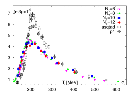
Since the trace anomaly is the central quantity in the lattice calculations of the EoS, we discuss its properties in some detail. In Fig. 1, we compare results for the trace anomaly obtained with the HISQ/tree action on lattices with temporal extent $N_{\tau}=6$, $8$, $10$, and $12$ with our previous findings using the p4 and asqtad actions Cheng et al. (2008); Bazavov et al. (2009); Petreczky (2009). The cutoff effects are much smaller in the HISQ/tree action and the height of the peak is significantly reduced. Below the peak, the HISQ/tree data are larger than the p4 and asqtad results, but significantly smaller at temperatures around and higher than the peak. These large deviations reflect the fact that the asqtad and the p4 actions have much larger cutoff effects at low temperatures and in the crossover region (see discussions in Ref. Bazavov et al. (2012a)). The smaller taste violations of the HISQ action lead to a smaller root-mean-square mass in the pseudoscalar sector Bazavov et al. (2012a), i.e., to a smaller average pion mass, which leads to a larger trace anomaly as well as larger pressure and energy density in the low temperature, hadronic region. For $T>350$ MeV, we find reasonably good agreement between the results obtained with different actions. This is, to some extent, expected as at such high temperatures, i.e., at small $a$, all the above actions should have small cutoff effects. This expectation has been demonstrated in the calculations of quark-number susceptibilities Bazavov et al. (2013b). In Sec. IV, we show that having small cutoff effects in the data with the HISQ/tree action allows us to make robust continuum extrapolations and obtain a precise EoS in the temperature range 130–400 MeV.

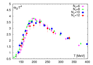
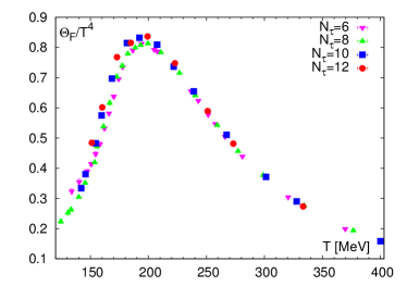
A closer look at the HISQ/tree action data shown in Figs. 1, 2, and 3 reveals some cutoff effects at low temperatures and in the peak region. It is instructive to discuss these cutoff effects separately in terms of the gluonic, $\Theta_{G}^{\mu\mu}$, and the fermionic, $\Theta_{F}^{\mu\mu}$, contributions defined in Eqs. (8) and (9), respectively, and shown in Fig. 2. We find that the trace anomaly is dominated by the gluonic part. The fermionic contribution is about $(20-25)\%$ of the gluonic contribution in the peak region, rises to $\sim 35\%$ below it, and becomes much smaller at high temperatures. At $T=400$ MeV, it is only about $10\%$. Around the peak, $\Theta_{G}^{\mu\mu}$, and consequently the trace anomaly, shows a decrease with increasing $N_{\tau}$, i.e., the continuum limit is approached from above.

The statistical errors and the lattice discretization effects in the HISQ/tree data are smaller in the fermionic part compared to the gluonic part. In $\Theta_{F}/T^{4}$, we observe significant cutoff effects only at the lowest temperature $T\sim 133$ MeV, where the $N_{\tau}=6$ and 8 data differ by about 30%. This small size of cutoff effects in $\Theta_{F}^{\mu\mu}$ with the HISQ/tree action in the low temperature region is in contrast to results obtained using the asqtad and the p4 actions, where the fermionic part showed significantly larger cutoff effects. We also note that cutoff effects arising from taste symmetry violations have opposite effects in $\Theta_{F}^{\mu\mu}$ and $\Theta_{G}^{\mu\mu}$. While a larger root-mean-square (RMS) mass for the pions leads to smaller values of $\Theta_{G}^{\mu\mu}$ at low temperatures, it leads to larger values in $\Theta_{F}^{\mu\mu}$ as the chiral condensates are larger for larger pion masses.

In the total trace anomaly, significant discretization effects are observed only in the peak and low-temperature regions. Within errors, we find no cutoff effects on comparing $N_{\tau}=6,\leavevmode\nobreak\ 8$, and $10$, data for $T<145$ MeV. In the interval $145\leavevmode\nobreak\ {\rm MeV}<T<170\leavevmode\nobreak\ {\rm MeV}$, we observe some cutoff dependence, with the largest difference between the $N_{\tau}=6$ and $8$ data.

Figure 3: The trace anomaly in the low temperature region compared with the hadron resonance gas model (solid line).

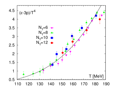
At low temperatures, all thermodynamic quantities are expected to be well-described by the hadron resonance gas (HRG) model, in which all the hadrons and hadron resonances are assumed to contribute to the thermodynamics as non-interacting particles. Many previous studies have confirmed this expectation Karsch et al. (2003); Cheng et al. (2009); Huovinen and Petreczky (2010); Borsanyi et al. (2010b); Borsanyi et al. (2012a); Bazavov et al. (2012b); Bazavov et al. (2013a). The trace anomaly in the HRG model is given by

$$\displaystyle\left(\frac{\epsilon-3p}{T^{4}}\right)^{HRG}=$$

$$\displaystyle\sum_{m_{i}\leq m_{max}}\frac{d_{i}}{2\pi^{2}}\sum_{k=1}^{\infty}\frac{(-\eta_{i})^{k+1}}{k}\left(\frac{m_{i}}{T}\right)^{3}K_{1}(\frac{km_{i}}{T})\;,$$ (13)

where different particle species of mass $m_{i}$ have degeneracy factors $d_{i}$ and $\eta_{i}=-1(+1)$ for bosons (fermions). The particle masses are taken from the Particle Data Book Beringer et al. (2012), including all known states up to the resonance mass of $m_{max}=2.5$ GeV. We compare the predictions of the HRG model with our data for the trace anomaly in the low temperature region in Fig. 3. For $T<145$ MeV the lattice data do not show any significant $N_{\tau}$ dependence and are in good agreement with estimates from the HRG model. This agreement will be used in an important way for the continuum extrapolation and for the calculation of the pressure described in the next section. For temperatures in the interval $145\leavevmode\nobreak\ {\rm MeV}<T<170\leavevmode\nobreak\ {\rm MeV}$, the $N_{\tau}=8,\leavevmode\nobreak\ 10$ and $12$ lattice data lie above the HRG curve, while the $N_{\tau}=6$ data lie systematically below. In Sec. IV, we show that the cutoff effects in the $N_{\tau}=6$ data are large in this temperature interval.

IV Thermodynamics in the continuum limit

In this section, we describe the calculation of the pressure and the energy and entropy densities in the continuum limit. The main step in this calculation is the extrapolation of the lattice data for the trace anomaly $\Theta^{\mu\mu}$ from $N_{\tau}=6$, $8$, $10$, and $12$ lattices to the continuum limit. Noting that the leading lattice discretization effects ($N_{\tau}$ dependence) for staggered fermions are expected to be proportional to $(aT)^{2}\sim 1/N_{\tau}^{2}$, we use the fit ansatz

$$\frac{\Theta^{\mu\mu}(T)}{T^{4}}=A+\sum_{i=1}^{n_{k}+3}B_{i}\times S_{i}(T)+\frac{C+\sum_{i=1}^{n_{k}+3}D_{i}\times S_{i}(T)}{N_{\tau}^{2}}\;,$$ (14)

where $n_{k}$ denotes the number of knots in the interior of the fit interval and the $S_{i}$ are a set of basis cubic splines with discontinuities only in the third derivative at the specified knots as described below. The positions of the knots and the constants $A,\ B_{i},\ C,$ and $D_{i}$ are parameters that are determined by the fit. To test whether it is sufficient to keep just the leading $1/N_{\tau}^{2}$ term, we also considered the next, $O(1/N_{\tau}^{4})$, correction,

$$\frac{E+\sum_{i=1}^{n_{k}+3}F_{i}\times S_{i}(T)}{N_{\tau}^{4}}\;.$$ (15)

Adding these terms to the quadratic fit, given in Eq. (14), defines the quartic fit also discussed below.

The basic assumption underlying the proposed fit ansatz is that the data and the variation with $N_{\tau}$ can be described by a set of piecewise continuous splines of cubic order. The temperature interval to be fitted is divided into sub-regions by a finite number of internal knots $n_{k}$, which we further assume are independent of $N_{\tau}$. The number and position of these knots specify a set of basis splines that forms a complete set over the full interval, i.e., any piecewise continuous cubic function can be fitted by them. The number of knots needed depends, in general, on the complexity of the data; and the total number of basis splines invoked by the fit depends on the number of knots specified. The positions of the knots are outputs of the least-square minimization procedure we use.

A number of choices need to be specified before we can discuss the fits.

• The errors in each data point for $\Theta^{\mu\mu}(T)/T^{4}$ are assumed to be normally distributed and independent, since these come from independent simulations.

• The entire analysis is done within a bootstrap procedure using 20,001 samples. This number was chosen to make the sampling error in the bootstrap estimate of the standard error $1\%$. The bootstrap samples were generated by selecting each data point from a normal distribution with its width given by the quoted error. The final error band for $\Theta^{\mu\mu}(T)/T^{4}$ is given by the $1\sigma$ spread of the bootstrap values at each temperature. The statistical package R R Core Team (2013); Venables and Ripley (2002); Jr et al. (2014) was used to implement this analysis.

• The values of temperature at which simulations have been done are not uniform, in particular we do not have much data on $N_{\tau}=10$ and $12$ lattices for $T<130$  MeV and $T>400$ MeV. Our results will, therefore, be restricted to the range $130\leavevmode\nobreak\ {\rm MeV}\leq T\leq 400$ MeV.

• Our goal is to use the minimum number of knots, and thus, the minimum number of parameters. We studied the $\chi^{2}$ resulting from the least-square minimization procedure to settle on the number of knots.

• We analyze the data using both the quadratic and quartic ansatz and with and without the $N_{\tau}=6$ data. Our final results are obtained using the quadratic fit without the $N_{\tau}=6$ data.

• The data on $N_{\tau}=8$ lattices for $T\leq 130$ MeV are insufficient to constrain the fits at the lower end. We, therefore, use the estimate $\Theta^{\mu\mu}(T)/T^{4}=1.007$ with slope $0.032$ at $T=130$ MeV, obtained from the HRG model, for the continuum extrapolated value. To justify this choice we note that the HRG model is a good approximation at this temperature and insensitive to possible higher resonances missed in the hadron spectrum Bazavov et al. (2014). Indeed, we find that the lattice data and the HRG estimates agree for $T<145$ MeV. To take into account the uncertainty in the HRG estimates, both the estimate and the slope were picked using a Gaussian distribution about their central values with a conservatively chosen width, $10\%$ of their respective values.We implemented this constrain by replacing the spline $B_{1}$ by a term proportional to $T-130$ MeV with its coefficient given by the HRG value. This constraint, therefore, reduces the number of free parameters in Eq. (14) by two.

• The data on $N_{\tau}=8$ lattices in the temperature range (400–610)/ MeV was used to stabilize the quadratic fits up to $400$ MeV. For the quartic fits, both the $N_{\tau}=6$ and $8$ data at $T>400$ MeV were used.

To decide on the number of knots to use, we fit the $N_{\tau}=8,\ 10$, and $12$ data with the quadratic ansatz with 2–4 internal knots. The fit with two knots was the most stable and the $\chi^{2}$ did not improve significantly with additional knots. The choice of two knots is consistent with the observation that the data show three main regions: the low temperature region $T\raise 1.29167pt\hbox{$<$\kern-7.5pt\raise-4.73611pt\hbox{$\sim$}}175$ MeV, the peak region (175–225 MeV) and the high temperature region $T\raise 1.29167pt\hbox{$>$\kern-7.5pt\raise-4.73611pt\hbox{$\sim$}}225$ MeV. The fit parameters and the location of the knots are outputs of the $\chi^{2}$ minimization procedure. This fit has 53 data points, 5 basis splines and 12 free parameters, i.e., the 10 parameters remaining in Eq. (14) after imposing the HRG value and slope at $T=130$ MeV and the locations of the two knots. This ansatz fits all the data, and the $\chi^{2}/{\rm dof}=0.9$ for ${\rm dof}=41$ was well distributed, $i.e.$, it was not dominated by a few points nor by any one of the three regions. The distribution of the positions of the knots over the 20,001 samples had central values of $170$ MeV and $229$ MeV with a standard deviation of 8 MeV. This fit, called the final fit, is used for our continuum results as the tests itemized below did not improve upon it:

• Adding more knots to the final fit did not improve the fit. The additional parameters were poorly determined, and in most bootstrap samples two or more knots were coincident.

• We added the $N_{\tau}=6$ data to the final fit. The $\chi^{2}/{\rm dof}$ increased and the fit became skewed. It adjusted to preferentially fit the low error $N_{\tau}=6$ points and the $\chi^{2}$ became dominated by the $N_{\tau}=12$ data below the peak. We concluded that the quadratic ansatz is insufficient to fit the data at all four $N_{\tau}$ values.

• We explored the quartic ansatz to fit the data at all four $N_{\tau}$ values. In this case, the best fit required three knots. The resulting error band overlaps with that of the the final fit except in the peak region, where it is about $1\sigma$ lower. The position of the knots are not as stable as in the final fit, and in many bootstrap samples, two knots were coincident. To summarize, the final quadratic fit was preferred over the quartic fit as it is based on data closer to the continuum limit, has the least number of parameters and fits the data well as shown in Fig. 4.

Figure 4: The data for the trace anomaly and the result (thick lines showing the $1\sigma$ bootstrap error bands) of applying Eq. (14) with $N_{\tau}=8$, $10$, and $12$. The parameters in Eq. (14) and their errors, defining this final fit, were determined from these data as discussed in the text. The error bands shown are generated by the same bootstrap process used to estimate the fit parameters and their errors. The additional $2\%$ error that is added to the final continuum result to account for the uncertainty in the determination of the temperature scale as discussed in the text is not included in these plots.

Figure 5: Spline fits to the trace anomaly for several values of the lattice spacing $aT=1/N_{\tau}$ and the result of our continuum extrapolation (left). Note that the error bands shown here do not include the 2% scale error. The right hand panel shows suitably normalized pressure, energy density, and entropy density as a function of the temperature. In this case the 2% scale error is included in the error bands. The dark lines show the prediction of the HRG model. The horizontal line at $95\pi^{2}/60$ in the right panel corresponds to the ideal gas limit for the energy density and the vertical band marks the crossover region, $T_{c}=(154\pm 9)$ MeV.

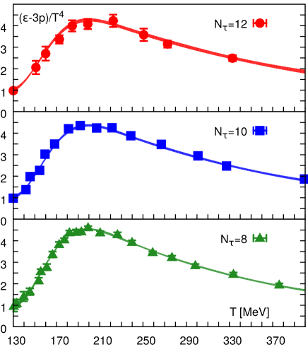
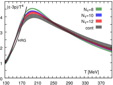
The quality of the final fit using Eq. (14) is demonstrated in Fig. 4 where we show that the bootstrap error bands of the final fit describe the $N_{\tau}=8$, $10$, and $12$ data very well. On the other hand, as stated previously, we find that the $N_{\tau}=6$ data lie outside the range of applicability of the quadratic ansatz. The same error bands are compared with the final continuum extrapolated result (black band) in Fig. 5.

Having determined the final fit, we obtained the pressure $p/T^{4}$ by numerically integrating the bootstrap samples for $\Theta^{\mu\mu}(T)$ between $130$ MeV and $400$ MeV using Eq. (12). For the integration constant $p_{0}$, the pressure at $T=130$ MeV, we picked a value from a normal distribution with the mean value $p_{0}/T_{0}^{4}=0.4391$, again taken from the HRG model, and width $0.0439$, a conservative $10\%$ error estimate on this HRG value. Since the estimate of $p_{0}/T_{0}^{4}$ is independent of the calculation of $\Theta^{\mu\mu}(T)$, this choice effectively adds a $\delta p_{0}$ in quadrature to the errors from integrating $\Theta^{\mu\mu}(T)/T^{4}$. Knowing $\Theta^{\mu\mu}(T)/T^{4}\equiv(\epsilon-3p)/T^{4}$ and $p/T^{4}$, it is straightforward to derive the energy density, $\epsilon$, and the entropy density $s=(\epsilon+p)/T$.

The final systematic error that is folded into the estimates of all the thermodynamic quantities is the uncertainty in the determination of the lattice scale $a$, and thus the values of the temperature $T$ used in the fits. Based on the uncertainty analyses in the determination of the lattice scale $a$ ($\sim 1.3\%$) and tuning of the $m_{s}$ to stay on the LCP presented in Appendices B and C, we assigned an overall conservative $2\%$ uncertainty in $T$, which we add linearly to the error estimates already assigned by the bootstrap process. In practice, at each $T$ and for each observable, we picked the minimum and maximum values of the $1\sigma$ bootstrap envelope in the region $T\pm 2\%$. This new envelope is then used as the final uncertainty band for all the continuum results shown in the figures and discussed below.

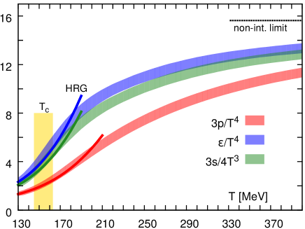
Our continuum extrapolated results for the trace anomaly and other thermodynamic observables are shown in Fig. 5 and the data are given in Table 1. For $T<150$ MeV, the trace anomaly is well approximated by the HRG estimate shown by the solid line in Fig. 5 (left). For $T>150$ MeV, the $N_{\tau}\geq 8$ lattice results are systematically higher than the HRG estimate as shown in Fig. 3, and the slopes of the HRG and continuum extrapolated curves start to differ as shown in Fig. 5. In the peak region, $(\epsilon-3p)/T^{4}$ has a maximum of about $4.05(15)$ at $T\sim 204$ MeV. This maximal value from simulations with the HISQ/tree action is significantly smaller than our previous results with the p4 and asqtad actions which were incorporated in the HotQCD parametrization Bazavov et al. (2009) of the EoS, as well as in the s95p parametrization of the EoS that is frequently used in hydrodynamic models Huovinen and Petreczky (2010).

$T[{\rm MeV}]$	$\Theta^{\mu\mu}/T^{4}$	$p/T^{4}$	$\epsilon/T^{4}$	$s/T^{3}$	$C_{V}/T^{3}$	$c_{s}^{2}$
130	1.01(-10)(+19)	0.439(-44)(+65)	2.33(-16)(+33)	2.77(-20)(+39)	16.5(-0.9)(+3.0)	0.168(-15)(+6)
135	1.21(-21)(+23)	0.481(-67)(+69)	2.65(-35)(+38)	3.13(-41)(+44)	20.4(-3.0)(+3.1)	0.153(-10)(+12)
140	1.46(-24)(+25)	0.529(-72)(+75)	3.05(-41)(+43)	3.58(-47)(+50)	24.5(-3.2)(+3.4)	0.146(-8)(+9)
145	1.76(-27)(+28)	0.586(-78)(+82)	3.52(-46)(+48)	4.11(-52)(+55)	28.6(-3.4)(+3.6)	0.144(-6)(+7)
150	2.09(-29)(+30)	0.651(-85)(+89)	4.05(-50)(+52)	4.70(-58)(+60)	32.6(-3.6)(+3.6)	0.144(-6)(+7)
155	2.43(-31)(+32)	0.726(-93)(+97)	4.61(-54)(+56)	5.34(-62)(+65)	36.2(-3.6)(+3.5)	0.148(-7)(+7)
160	2.76(-32)(+32)	0.808(-100)(+105)	5.19(-57)(+59)	6.00(-66)(+68)	39.3(-3.4)(+3.3)	0.153(-8)(+9)
165	3.07(-32)(+31)	0.898(-108)(+112)	5.76(-59)(+60)	6.66(-69)(+70)	41.8(-3.2)(+3.0)	0.159(-9)(+10)
170	3.34(-31)(+30)	0.994(-115)(+118)	6.32(-60)(+60)	7.32(-70)(+71)	43.8(-2.9)(+2.7)	0.167(-10)(+10)
175	3.56(-29)(+28)	1.094(-121)(+124)	6.85(-60)(+60)	7.94(-71)(+71)	45.2(-2.6)(+2.4)	0.176(-11)(+10)
180	3.74(-27)(+25)	1.197(-126)(+129)	7.33(-59)(+59)	8.53(-71)(+70)	46.2(-2.4)(+2.1)	0.185(-11)(+10)
185	3.88(-25)(+23)	1.302(-130)(+133)	7.78(-58)(+57)	9.08(-71)(+71)	47.0(-2.2)(+1.9)	0.194(-11)(+10)
190	3.97(-22)(+19)	1.406(-134)(+136)	8.19(-57)(+56)	9.60(-69)(+68)	47.5(-1.9)(+1.7)	0.202(-10)(+10)
195	4.03(-19)(+16)	1.510(-137)(+139)	8.56(-56)(+54)	10.07(-68)(+67)	47.9(-1.7)(+1.6)	0.210(-10)(+10)
200	4.05(-16)(+14)	1.613(-140)(+141)	8.89(-54)(+52)	10.50(-67)(+65)	48.1(-1.6)(+1.5)	0.218(-10)(+10)
205	4.05(-14)(+14)	1.713(-142)(+143)	9.19(-52)(+50)	10.90(-65)(+63)	48.4(-1.5)(+1.6)	0.225(-10)(+10)
210	4.03(-15)(+15)	1.810(-143)(+143)	9.46(-50)(+48)	11.27(-64)(+62)	48.6(-1.6)(+1.6)	0.232(-10)(+10)
215	3.99(-16)(+16)	1.904(-144)(+144)	9.70(-48)(+47)	11.61(-62)(+60)	48.8(-1.6)(+1.7)	0.238(-10)(+9)
220	3.94(-17)(+17)	1.995(-144)(+144)	9.93(-47)(+46)	11.92(-61)(+59)	49.1(-1.7)(+1.8)	0.243(-9)(+9)
225	3.88(-18)(+17)	2.083(-145)(+144)	10.13(-46)(+45)	12.21(-59)(+58)	49.4(-1.8)(+1.8)	0.247(-9)(+8)
230	3.82(-18)(+18)	2.168(-145)(+144)	10.32(-45)(+44)	12.49(-59)(+58)	49.8(-1.8)(+1.9)	0.251(-8)(+8)
235	3.76(-19)(+18)	2.249(-144)(+143)	10.50(-45)(+44)	12.75(-59)(+58)	50.3(-1.9)(+1.9)	0.254(-8)(+7)
240	3.69(-19)(+19)	2.328(-144)(+143)	10.68(-44)(+44)	13.00(-58)(+58)	50.7(-1.9)(+1.9)	0.256(-8)(+7)
245	3.63(-20)(+19)	2.403(-144)(+143)	10.84(-44)(+44)	13.24(-58)(+57)	51.1(-1.9)(+1.9)	0.259(-7)(+7)
250	3.57(-20)(+20)	2.476(-143)(+142)	10.99(-44)(+44)	13.47(-57)(+57)	51.5(-1.9)(+1.9)	0.261(-7)(+6)
255	3.50(-21)(+20)	2.546(-143)(+142)	11.14(-44)(+44)	13.68(-57)(+57)	51.9(-1.9)(+1.9)	0.264(-7)(+6)
260	3.44(-21)(+21)	2.613(-143)(+142)	11.28(-44)(+44)	13.89(-58)(+57)	52.2(-1.9)(+1.9)	0.266(-7)(+6)
265	3.38(-21)(+21)	2.678(-142)(+141)	11.41(-44)(+44)	14.09(-58)(+57)	52.5(-1.9)(+1.8)	0.268(-6)(+6)
270	3.32(-21)(+21)	2.741(-142)(+141)	11.54(-44)(+44)	14.28(-57)(+57)	52.8(-1.8)(+1.8)	0.270(-6)(+6)
275	3.26(-21)(+21)	2.801(-141)(+141)	11.66(-44)(+44)	14.46(-57)(+57)	53.1(-1.8)(+1.8)	0.272(-6)(+5)
280	3.20(-21)(+21)	2.859(-141)(+140)	11.77(-44)(+43)	14.63(-57)(+57)	53.3(-1.8)(+1.7)	0.274(-6)(+5)
285	3.14(-21)(+21)	2.915(-141)(+140)	11.88(-43)(+43)	14.80(-57)(+57)	53.6(-1.8)(+1.7)	0.276(-5)(+5)
290	3.08(-21)(+21)	2.969(-140)(+140)	11.99(-43)(+43)	14.95(-57)(+56)	53.8(-1.7)(+1.7)	0.278(-5)(+5)
295	3.02(-20)(+21)	3.021(-140)(+140)	12.08(-43)(+43)	15.11(-56)(+56)	54.0(-1.7)(+1.7)	0.280(-5)(+5)
300	2.96(-20)(+21)	3.072(-140)(+139)	12.18(-43)(+43)	15.25(-56)(+56)	54.2(-1.7)(+1.7)	0.282(-5)(+6)

Table 1: Continuum extrapolated results for the trace anomaly $\Theta^{\mu\mu}$, pressure $p$, energy density $\epsilon$, entropy density $s$, specific heat $C_{V}$, and the square of the speed of sound $c_{s}^{2}$ in appropriate units of the temperature $T$. The asymmetry in the errors, given in the two brackets, arises from the 2% systematic error in asigned to the temperature scale.

$T[{\rm MeV}]$	$\Theta^{\mu\mu}/T^{4}$	$p/T^{4}$	$\epsilon/T^{4}$	$s/T^{3}$	$C_{V}/T^{3}$	$c_{s}^{2}$
305	2.91(-20)(+21)	3.120(-139)(+139)	12.27(-43)(+42)	15.39(-56)(+55)	54.3(-1.7)(+1.7)	0.283(-5)(+6)
310	2.85(-20)(+20)	3.167(-139)(+139)	12.35(-42)(+42)	15.52(-56)(+55)	54.5(-1.7)(+1.7)	0.285(-6)(+6)
315	2.79(-19)(+20)	3.212(-139)(+138)	12.43(-42)(+42)	15.64(-56)(+55)	54.6(-1.7)(+1.7)	0.286(-6)(+6)
320	2.74(-19)(+20)	3.256(-139)(+138)	12.51(-42)(+41)	15.76(-55)(+55)	54.8(-1.7)(+1.7)	0.288(-6)(+6)
325	2.69(-19)(+20)	3.298(-138)(+138)	12.58(-42)(+41)	15.88(-55)(+54)	54.9(-1.7)(+1.7)	0.289(-6)(+7)
330	2.63(-19)(+19)	3.338(-138)(+137)	12.65(-41)(+41)	15.99(-54)(+54)	55.0(-1.7)(+1.7)	0.291(-6)(+7)
335	2.58(-19)(+19)	3.377(-138)(+137)	12.71(-41)(+41)	16.09(-54)(+54)	55.1(-1.7)(+1.8)	0.292(-6)(+7)
340	2.53(-19)(+19)	3.415(-137)(+137)	12.78(-41)(+40)	16.19(-54)(+53)	55.2(-1.7)(+1.8)	0.293(-7)(+7)
345	2.48(-20)(+19)	3.452(-137)(+136)	12.83(-41)(+40)	16.29(-54)(+53)	55.3(-1.7)(+1.8)	0.294(-7)(+7)
350	2.43(-20)(+19)	3.487(-136)(+136)	12.89(-40)(+40)	16.38(-53)(+53)	55.4(-1.8)(+1.9)	0.296(-7)(+7)
355	2.38(-20)(+19)	3.521(-136)(+135)	12.94(-40)(+40)	16.47(-53)(+53)	55.5(-1.8)(+1.9)	0.297(-7)(+7)
360	2.33(-20)(+20)	3.554(-136)(+135)	13.00(-40)(+40)	16.55(-53)(+53)	55.6(-1.8)(+1.9)	0.298(-7)(+7)
365	2.29(-21)(+20)	3.586(-135)(+134)	13.04(-40)(+40)	16.63(-53)(+53)	55.7(-1.9)(+1.9)	0.299(-7)(+7)
370	2.24(-21)(+20)	3.617(-135)(+134)	13.09(-40)(+40)	16.71(-53)(+53)	55.8(-1.9)(+2.0)	0.300(-7)(+7)
375	2.20(-21)(+20)	3.647(-134)(+134)	13.14(-40)(+40)	16.78(-53)(+53)	55.8(-1.9)(+2.0)	0.301(-7)(+7)
380	2.15(-22)(+21)	3.675(-134)(+133)	13.18(-40)(+40)	16.85(-53)(+53)	55.9(-2.0)(+2.0)	0.302(-7)(+7)
385	2.11(-22)(+21)	3.703(-134)(+133)	13.22(-40)(+41)	16.92(-53)(+53)	56.0(-2.0)(+2.0)	0.302(-7)(+7)
390	2.07(-22)(+21)	3.730(-133)(+132)	13.26(-40)(+41)	16.99(-53)(+53)	56.1(-2.0)(+2.1)	0.303(-7)(+7)
395	2.03(-22)(+22)	3.756(-133)(+132)	13.30(-40)(+41)	17.05(-53)(+53)	56.2(-2.0)(+2.1)	0.304(-7)(+7)
400	1.99(-22)(+22)	3.782(-132)(+132)	13.34(-40)(+41)	17.12(-53)(+53)	56.2(-2.1)(+2.1)	0.304(-7)(+7)

Table 1 continued

The final continuum extrapolated estimates of the pressure, energy density and entropy density are shown in Fig. 5 (right) and compared with HRG predictions for $T<170$ MeV. Again, there is reasonable agreement for $T<150$ MeV. Above $T=150$ MeV, HRG estimates lie along the lower edge of the error-band of the lattice estimates.

Figure 6: The comparison of the HISQ/tree and stout results for the trace anomaly, the pressure, and the entropy density.

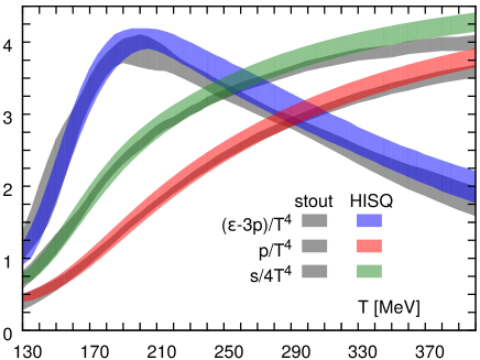
We can now compare our results with the results obtained by the Wuppertal-Budapest Collaboration using the stout action Borsanyi et al. (2014). This comparison is shown in Fig. 6 for the trace anomaly, the pressure and the entropy density. We find good agreement in the trace anomaly with the stout results over the full temperature range ($130-400$) MeV. Note, however, that above the peak the central values with the stout action lie systematically below ours. As a result, our estimates of the pressure become systematically larger for $T>200$ MeV. By $T=400$ MeV, the difference between the central values in the two calculations increases to about $6\%$. The two results, however, still agree within errors. The difference in the entropy density reaches about $7\%$ by $T=400$ MeV, and in this case the two estimates differ by about $2\sigma$. These differences suggest that more detailed calculations of the trace anomaly at higher temperatures are needed. In particular, it would be important to see if the differences persist at higher temperatures where a comparison with resummed perturbative calculations should be possible (see Sec. V.C).

IV.1 Parametrization of the equation of state

We close this section by providing an analytical parametrization of the pressure of (2+1)-flavor QCD, summarized in Table 1, that can be used in phenomenological applications and hydrodynamic modeling of strong interaction matter. We choose an ansatz that incorporates basic features of the low and high temperature limits, i.e., it ensures that the pressure becomes exponentially small at low temperatures and approaches the ideal gas limit at high temperatures. We find that the following parametrization provides an excellent description of all bulk thermodynamic observables discussed in the previous sections, including the specific heat and speed of sound that require second derivatives of $p/T^{4}$ with respect to the temperature to be discussed in the next section,

$$\frac{p}{T^{4}}=\frac{1}{2}\left(1+\tanh(c_{t}(\bar{t}-t_{0}))\right)\cdot$$

$$\frac{p_{id}+a_{n}/\bar{t}+b_{n}/\bar{t}^{2}+c_{n}/\bar{t}^{3}+d_{n}/\bar{t}^{4}}{1+a_{d}/\bar{t}+b_{d}/\bar{t}^{2}+c_{d}/\bar{t}^{3}+d_{d}/\bar{t}^{4}}\;,$$ (16)

where $\bar{t}=T/T_{c}$ and the QCD transition temperature $T_{c}=154$ MeV is a conveniently chosen normalization. In this parametrization, $p_{id}=95\pi^{2}/180$ is the ideal gas value of $p/T^{4}$ for massless 3-flavor QCD. It is also the appropriate infinite temperature limiting value for QCD with light and strange quarks that could be refined to include additional perturbative corrections. However, at present we do not see any need for this. We also note that fixing $c_{n}=c_{d}=0$ gives an excellent parametrization of all our numerical data and is in good agreement with the HRG estimate, at least down to $T=100$ MeV. Furthermore, this parametrization agrees with the $N_{\tau}=8$ data well beyond $T=400$ MeV.

$c_{t}$	$a_{n}$	$b_{n}$	$c_{n}$	$d_{n}$
3.8706	-8.7704	3.9200	0	0.3419
$t_{0}$	$a_{d}$	$b_{d}$	$c_{d}$	$d_{d}$
0.9761	-1.2600	0.8425	0	-0.0475

Table 2: Parameters used in the ansatz given in Eq. (16) for the pressure of (2+1)-flavor QCD in the temperature interval $T\in[100\leavevmode\nobreak\ {\rm MeV},400\leavevmode\nobreak\ {\rm MeV}]$.

The values of the parameters in our ansatz for the pressure, Eq. (16), are summarized in Table 2. The results of this ansatz for the speed of sound, energy density, and specific heat are compared with our continuum extrapolated error bands in Figs. 7 and 8.

V Specific heat, the speed of sound and deconfinement

All thermodynamic quantities, for fixed light and strange quark masses, depend on a single parameter—the temperature. In Section IV, we derived the basic thermodynamic observables ($\epsilon,\leavevmode\nobreak\ p,\leavevmode\nobreak\ s$) from the continuum extrapolated trace anomaly $\Theta^{\mu\mu}(T)$. We now discuss two closely related observables that involve second order derivatives of the QCD partition function with respect to the temperature, i.e., the specific heat,

$$C_{V}=\left.\frac{\partial\epsilon}{\partial T}\right|_{V}\equiv\left(4\frac{\epsilon}{T^{4}}+T\left.\frac{{\partial}(\epsilon/T^{4})}{\partial T}\right|_{V}\right)T^{3}\,,$$ (17)

and the speed of sound,

$$c_{s}^{2}=\frac{\partial p}{\partial\epsilon}=\frac{\partial p/\partial T}{\partial\epsilon/\partial T}=\frac{s}{C_{V}}\;.$$ (18)

The quantity $T{{\rm d}(\epsilon/T^{4})}/{{\rm d}T}$ can be calculated directly from the trace anomaly and its derivative with respect to temperature,

$$T\frac{{\rm d}\epsilon/T^{4}}{{\rm d}T}=3\frac{\Theta^{\mu\mu}}{T^{4}}+T\frac{{\rm d}\Theta^{\mu\mu}/T^{4}}{{\rm d}T}\;.$$ (19)

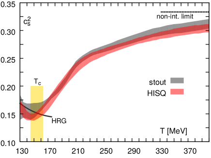
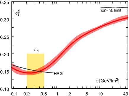
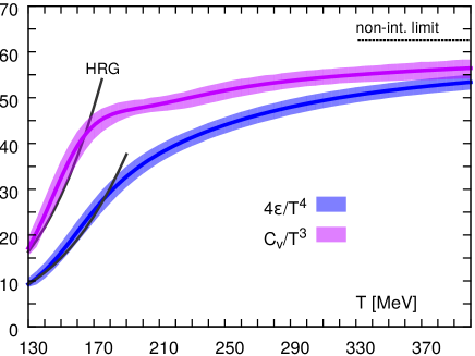
These identities show that the estimates for the specific heat and the speed of sound should be of a quality similar to $\epsilon/T^{4}$ or $p/T^{4}$. In Figs. 7 and 8, we show the agreement between the bootstrap error bands for these quantities and the estimates obtained by taking second order derivatives of the analytic parameterization for $p/T^{4}$ given in Eq. 16. The latter are shown as dark lines inside the bootstrap error bands.

Figure 7: The speed of sound squared from lattice QCD and the HRG model versus temperature (top) and energy density (bottom). In the upper figure, our results (HISQ) are compared with those obtained with the stout action Borsanyi et al. (2014). The vertical band marks the location of the crossover region $T_{c}=(154\pm 9)$ MeV in the upper figure and the corresponding range in energy density , $\epsilon_{c}=(0.18-0.5)\leavevmode\nobreak\ {\rm GeV/fm}^{3}$, in the lower figure. The dark line within each error band is the prediction of the analytical parameterization given in Eq. (16).

V.1 Speed of sound, the softest point of the EoS and the critical energy density

In Fig. 7 (top), we show the speed of sound as a function of the temperature and compare our results with those obtained by using the stout action Borsanyi et al. (2014). We find that the HISQ/tree and the stout results agree within the estimated errors. The softest point of the EoS Hung and Shuryak (1995) at $T\simeq(145-150)$ MeV, i.e., at the minimum of the speed of sound, lies on the low temperature side of the crossover region. At this point, the speed of sound is only slightly below the corresponding HRG value. This follows from the good agreement between HRG estimates and our lattice QCD results for the energy density and the pressure. Furthermore, the value $c_{s}^{2}\simeq 0.15$ is roughly half way between zero, the value expected at a second order phase transition with diverging specific heat, and the value for an ideal massless gas, $c_{s}^{2}=1/3$. At the high temperature end, $T\sim 350$ MeV, it reaches within $10\%$ of the ideal gas value.

The softest point of the EoS is of interest in the phenomenology of heavy ion collisions as it characterizes the temperature and energy density range in which the expansion and cooling of matter slows down. The system spends a longer time in this temperature range, and one expects to observe characteristic signatures from this regime. To facilitate a more direct comparison with experiments, we show $c_{s}^{2}$ as a function of the energy density in physical units in Fig. 7 (bottom) using the parametrization given in Eq. 16 to convert temperature to energy density. At the softest point, the energy density is only slightly above that of normal nuclear matter, $\epsilon_{\rm nuclear}=150\leavevmode\nobreak\ {\rm MeV}/{\rm fm}^{3}$. In the crossover region, $T_{c}=(154\pm 9)$ MeV Bazavov et al. (2012a), the energy density varies from $180\leavevmode\nobreak\ {\rm MeV}/{\rm fm}^{3}$ at the lower edge to $500\leavevmode\nobreak\ {\rm MeV}/{\rm fm}^{3}$ at the upper edge, slightly above the energy density inside the proton $\epsilon_{\rm proton}=\leavevmode\nobreak\ 450\leavevmode\nobreak\ {\rm MeV}/{\rm fm}^{3}$.

The QCD crossover region, thus, starts at or close to the softest point of the EoS and the entire crossover region corresponds to relatively small values of the energy density, $(1.2-3.1)\epsilon_{\rm nuclear}$. This value is about a factor of four smaller than that of an ideal quark-gluon gas in this temperature range. In the next subsection, we will discuss to what extent this has consequences for the size of fluctuations in the energy density, i.e., the specific heat.

V.2 Specific heat and deconfinement

The intuitive characterization of deconfinement at the QCD phase transition is that the liberation of many new degrees of freedom give rise to a rapid increase in the energy density, ideally with an infinite slope at $T_{c}$ as in a conventional second order phase transition. This rapid rise would then show up as a peak (or even a divergence) in the specific heat, which could serve as an indicator for the pseudo-critical (or critical) temperature. However, the specific heat of (2+1)-flavor QCD, shown in Fig. 8, exhibits a rapid increase but no peak. In the crossover region, $C_{V}/\epsilon\simeq 8/T$ is a factor of two larger than for an ideal quark-gluon gas; the specific heat reaches about half of its ideal gas value, $(C_{V}/T^{3})_{ideal}=4(\epsilon/T^{4})_{ideal}=95\pi^{2}/15$; and the energy density reaches only about one quarter of its limiting high temperature, ideal gas value.

Figure 8: Error bands showing the continuum extrapolation of the specific heat and energy density and solid lines obtained from the parametrization given in Eq. (16). Also shown are the HRG estimates at low temperatures and the ideal gas limit at high temperatures.

The analysis of the quark-mass dependence of the QCD transition temperature, the chiral condensate and, in particular, the peak in the chiral susceptibility suggest that for physical values of the quark masses QCD is sufficiently close to the chiral limit to be sensitive to the chiral phase transition Bazavov et al. (2012a) and exhibit an almost universal, pseudo-critical behavior controlled by it. The peak observed in the chiral susceptibility is dominated by the second derivative of the singular part of the free energy with respect to the quark mass Bazavov et al. (2012a). Extending that generic scaling analysis, one may have expected that, for physical quark masses, the pseudo-critical behavior would also lead to large fluctuations in the energy density and that the specific heat would exhibit a peak in the crossover region controlled by the second derivative with respect to temperature of the same singular part of the free energy.

There may be at least two reasons for the difference in behavior between the chiral susceptibility and the specific heat, which are second derivatives of the partition function with respect to the quark mass and the temperature, respectively. First, thermal fluctuations are controlled by the thermal critical exponent $\alpha$, i.e., $C_{V}/T^{3}\sim|T-T_{c}|^{-\alpha}$. In the 3-d $O(4)$ universality class, which is relevant for the chiral phase transition, the exponent $\alpha\simeq-0.21$ is negative Engels and Karsch (2012). Consequently, unlike the chiral susceptibility, the specific heat stays finite at $T_{c}$ even in the chiral limit. The singular part of the free energy Engels and Karsch (2012), which gives the leading temperature dependence in the vicinity of $T_{c}$, contributes only a cusp in $C_{V}$. This can be seen by examining the energy density near $T_{c}$,

$$\frac{\epsilon}{T^{4}}=e_{0}+e_{1}\left(\frac{T-T_{c}}{T_{c}}\right)+{\cal O}\left(|T-T_{c}|^{1-\alpha}\right)\;,$$ (20)

where the dominant contribution, $e_{0}$, comes from the regular part and the singular contributions, $\sim|T-T_{c}|^{1-\alpha}$, are sub-dominant. From Eq. (17), we get

$$\frac{C_{V}}{T^{3}}=c_{0}+\frac{A^{\pm}}{\alpha}\left|\frac{T-T_{c}}{T_{c}}\right|^{-\alpha}+{\cal O}\left(T-T_{c}\right)\;,$$ (21)

with $c_{0}=4e_{0}+e_{1}$ and $A^{+}$ ($A^{-}$) are the amplitudes above (below) $T_{c}$. The ratio of these amplitudes is universal and positive; $A^{+}/A^{-}=1.842(43)$ in the 3-d O(4) universality class Engels and Karsch (2012). Since $\alpha$ is negative, the singular part gives only a cusp, which should persist in the chiral limit but may not be easy to detect if the regular contributions are large.

The second reason for the lack of a peak in $C_{V}/T^{3}$ is that the contributions from the regular part of the free energy are large in the high temperature phase Engels and Karsch (2012), and are ${\cal O}(g^{0})$ at infinite temperature. Furthermore, as discussed above, the regular terms dominate even in the crossover region. To make this observation more explicit, we note from Eq. (17) that $C_{V}/T^{3}$ can be written in terms of the energy density, $\epsilon/T^{4}$, and its derivative,

$$T\frac{{\rm d}\epsilon/T^{4}}{{\rm d}T}\equiv\frac{\overline{C}_{V}}{T^{3}}\;.$$ (22)

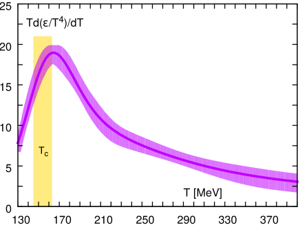
The dominant singular terms are contained in the second term ($\overline{C}_{V}/T^{3}$) or, more specifically, in the temperature derivative of the trace anomaly, i.e., the second term in Eq. (19). The contribution of the regular terms to $\overline{C}_{V}/T^{3}$ is strongly suppressed at high temperatures; it is zero in the infinite temperature ideal gas limit and receives contributions starting at ${\cal O}(g^{4})$ in perturbation theory. Thus, while $C_{V}$ and $\overline{C}_{V}$ have identical leading contributions from the singular part near $T_{c}$, the contribution from the regular part is much smaller in $\overline{C}_{V}$. Consequently, the singular behavior is not masked and $\overline{C}_{V}$ has a pronounced peak close to the chiral crossover region as shown in Fig. 9. To summarize, the location of the peak in the temperature derivative of $\epsilon/T^{4}$ is a good indicator of deconfinement, i.e., the liberation of quark-gluon degrees of freedom, and occurs close to the chiral transition in QCD as shown in Fig. 9.

Figure 9: Derivative of $\epsilon/T^{4}$ with respect to temperature. The vertical band gives the chiral crossover temperature determined from the location of the peak in the disconnected chiral susceptibility.

V.3 Approach to the perturbative limit

In this subsection, we discuss how our results for the (2+1)-flavor EoS connect to analytic calculations at high temperatures.

At sufficiently high temperatures, thermodynamics should be describable in terms of a weakly interacting quark-gluon gas, and at infinite temperature all thermodynamic quantities will converge to the ideal gas limit. Plots in Fig. 5 show that at our highest temperature value, $T=400$ MeV, the entropy and energy density and pressure are still $13\%$, $18\%$ and $27\%$, respectively, below the ideal gas limit. In contrast to other quantities, e.g., susceptibilities of conserved charge fluctuations, these deviations from the ideal gas limit are still quite large. This is probably due to large nonperturbative contributions in the gluonic sector of QCD which are present in bulk thermodynamic observables but are suppressed in observables that, at tree level, only depend on the quark sector of QCD.

Although, for some observables, resummation Haque et al. (2014) or dimensional reduction Laine and Schroder (2006) based perturbative calculations show good agreement with lattice QCD calculations already at temperatures $T\sim 400$ MeV, for others this is not the case. In particular, their functional dependence on temperature is still significantly different in this temperature range, which can lead to larger differences in higher order derivatives between perturbative and lattice QCD calculations. As our current continuum-extrapolated EoS is limited to $T<400$ MeV, we cannot perform a detailed comparison with perturbation theory but point out a few qualitative features.

We have shown in Fig. 6 that continuum-extrapolated results for the trace anomaly obtained with the stout and the HISQ discretization schemes agree within errors. At high temperatures, however, the HISQ results are systematically above the stout results. This propagates into other thermodynamic observables, e.g., the pressure. The systematic differences, however, cancel to a large extent in ratios. For example, the ratio of the trace anomaly and the pressure,

$$\frac{\Theta^{\mu\mu}}{p}=\frac{\epsilon}{p}-3\;,$$ (23)

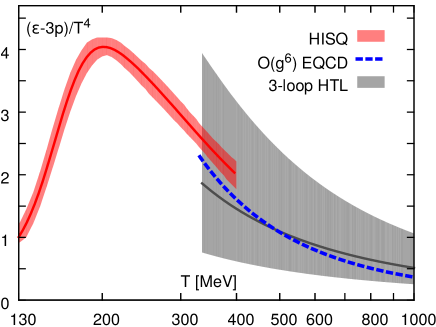
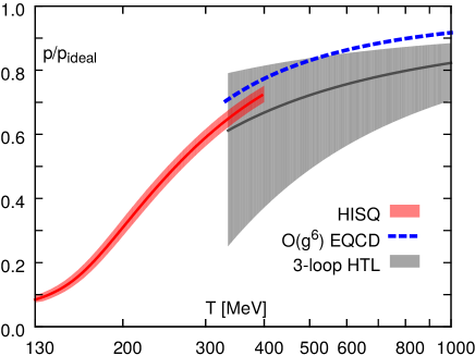
is in excellent agreement between the two calculations and thus provides a good starting point for a comparison with high temperature perturbative calculations. In Fig. 10, we show results for the ratio $\Theta^{\mu\mu}/p$ and compare with perturbative calculations performed in the Hard Thermal Loop (HTL) Haque et al. (2014) and Electrostatic QCD (EQCD) Laine and Schroder (2006) schemes. The broad band for the three-loop HTL calculation corresponds to varying the renormalization scale in the interval $\mu=(1-4)\pi T$ and the black line in this band corresponds to $\mu=2\pi T$. The EQCD and HTL results for $\mu=2\pi T$ are in good agreement, and the lattice QCD results approach these estimates for $T\raise 1.29167pt\hbox{$>$\kern-7.5pt\raise-4.73611pt\hbox{$\sim$}}500$ MeV.

Figure 10: The ratio of the trace anomaly and the pressure from (2+1)-flavor QCD calculations with the HISQ and stout actions, respectively. These results are compared to HTL and EQCD (dashed line) calculations. The black line corresponds to the HTL calculation with renormalization scale $\mu=2\pi T$.

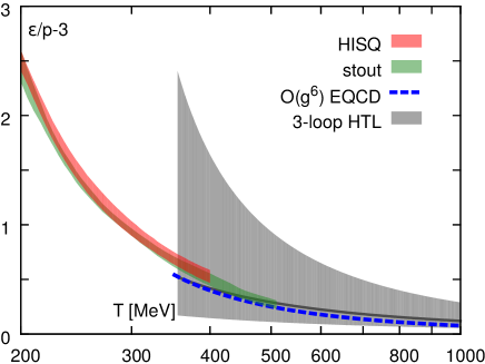
In Fig. 11, we compare the three-loop HTL estimates with lattice QCD calculations of the trace anomaly (top) and the pressure (bottom). Also shown, with a dashed line in Figs. 10 and 11, is the result of an ${\cal O}(g^{6})$ calculation performed in the dimensional reduction scheme (EQCD). The lattice QCD results are in qualitative agreement with these perturbative calculations, with the ${\cal O}(g^{6})$ EQCD estimate lying below the lattice QCD results for the trace anomaly and above for the pressure at $T=400$ MeV.

One could try fixing the scale uncertainty in the HTL calculation by matching one of the observables to the lattice QCD result, e.g., the pressure. Results for other observables, e.g., the trace anomaly would then be parameter free predictions. It is clear from Fig. 11 that such a simultaneously agreement between HTL and lattice QCD calculations of $p/T^{4}$ and $(\epsilon-3p)/T^{4}$ is not forthcoming. Making the HTL and the lattice QCD estimates agree for the trace anomaly by reducing the value for the renormalization scale $\mu$ would decrease the HTL results for $p/T^{4}$ even further and, thereby, increase the deviation from the lattice QCD results.

Lastly, the EQCD result for the pressure in the temperature range $(400-1000)$ MeV is about 10% larger than the HTL result with $\mu=2\pi T$. To resolve the open question whether at these high temperatures the pressure obtained from lattice QCD calculations is better described by the HTL or the EQCD calculations requires lattice simulations at higher temperatures.

Figure 11: Comparison of the (2+1)-flavor calculation of the trace anomaly (top) and pressure (bottom) with HTL and EQCD (dashed line) calculations. The black line corresponds to the HTL calculation with renormalization scale $\mu=2\pi T$. Note that this solid line would move up for the trace anomaly and move down for the pressure if the scale $\mu$ in HTL is reduced.

VI Conclusions

We have calculated the trace anomaly and the equation of state in (2+1)-flavor QCD with almost physical quark masses using the HISQ/tree action on lattices with temporal extent $N_{\tau}=6,\leavevmode\nobreak\ 8,\leavevmode\nobreak\ 10$, and $12$. We find that the lattice discretization errors in the HISQ/tree action are small, and we obtain reliable continuum extrapolated results for a number of thermodynamic quantities for $130\leavevmode\nobreak\ {\rm MeV}<T<400\leavevmode\nobreak\ {\rm MeV}$. In fact, the trace anomaly calculated on the $N_{\tau}=12$ lattices agrees with the continuum-extrapolated results within errors. Our main results are summarized in Figs. 1, 5, and 6. Based on these results, we propose in Eq. 16 an analytical parameterization of the pressure for use in phenomenological studies that matches the HRG estimates below $T=130$ MeV and the lattice data between $(130-400)$ MeV.

We have compared our new results obtained using the HISQ/tree action with our previous calculations performed using the asqtad and the p4 actions Bazavov et al. (2009), and with the recent continuum extrapolated stout results Borsanyi et al. (2014). For $T<300$ MeV, the HISQ/tree results are very different from the results obtained using the p4 and the asqtad actions on $N_{\tau}=8$ lattices, $i.e.$, without an extrapolation to the continuum limit. At higher temperatures, the results show reasonable agreement as expected since all three actions have small lattice artifacts.

Results for our continuum extrapolated trace anomaly presented in Sec. IV agree well with those from the stout action Borsanyi et al. (2014). The discrepancy between the HotQCD results and the stout results discussed in Bazavov et al. (2009); Borsanyi et al. (2014) was due to the large cutoff effects in the previous estimates with the p4 and the asqtad actions and because our earlier results had not been extrapolated to the continuum limit.

We find reasonably good agreement for the pressure obtained using the stout and the HISQ/tree actions for $T<300$ MeV as shown in Fig. 6. At higher temperatures, there is some tension between the two estimates because the results for the trace anomaly, $\Theta^{\mu\mu}(T)/T^{4}$, obtained with the HISQ/tree action lie systematically above those from the stout action. Consequently, the pressure, which is the integral of $\Theta^{\mu\mu}(T)/T^{5}$, will start to differ significantly at high temperatures if the observed trends persist. In this paper, we focused on the temperature region $130\leavevmode\nobreak\ {\rm MeV}<T<400\leavevmode\nobreak\ {\rm MeV}$, which is the most relevant for phenomenological applications. Over this temperature range, the difference is unlikely to have a significant effect on the modeling of the hydrodynamic evolution of the system produced in heavy ion collisions (see the discussion in Ref. Huovinen and Petreczky (2010)). It is important to check, however, if this tension persists at higher temperatures, especially if one wants to determine to what extent the quark-gluon plasma is strongly or weakly coupled by comparing lattice and resummed perturbation theory results for the pressure or for the entropy density. Such calculations are left for future studies.

Appendix A HISQ ensembles and topological charge history

A.1 HISQ ensembles

To simulate the HISQ/tree action, we use the same Rational Hybrid Monte Carlo algorithm Clark et al. (2005) with mass preconditioning Hasenbusch (2001) as in the previous study Ref. Bazavov et al. (2012a). Details of these simulations are given in Ref. Bazavov et al. (2010b) and in Table 3 we present the key lattice parameters of our simulation, namely the gauge coupling $\beta=10/g^{2}$, the quark masses, the lattice dimensions, the accumulated statistics in terms of molecular dynamics time units (TU), and the length of the trajectories. The zero temperature lattices were saved every 5 TUs (or 6 TU for the fine lattices), and the finite temperature lattices were saved every 10 TUs.

			$T=0$			$N_{\tau}=6$	$N_{\tau}=8$	$N_{\tau}=10$	$N_{\tau}=12$
$\beta$	$m_{l}$	$m_{s}$	$N_{s}^{3}\times N_{\tau}$	$TU$	length	$TU$	$TU$	$TU$	$TU$
5.900	0.00660	0.1320	$24^{3}\times 32$	3700	1/4	30290	—	—	—
5.950	0.00615	0.1230	$24^{3}\times 32$	4715	1/4	30990	—		—
6.000	0.00569	0.1138	$24^{3}\times 32$	4890	1/3	31730	—	—	—
6.025	0.00550	0.1100	$24^{3}\times 32$	5250	1/3	33990	—	—	—
6.050	0.00532	0.1064	$24^{3}\times 32$	4655	1/3	32100	74210	—	—
6.075	0.00518	0.1036	$24^{3}\times 32$	4085	1/3	32990	—	—	—
6.100	0.00499	0.0998	$28^{3}\times 32$	4190	1/3	39900	—	—	—
6.125	0.00483	0.0966	$32^{4}$	8645	1/3	32990	67720	—	—
6.150	0.00468	0.0936	$24^{3}\times 32$	7795	1/3	31130	—	—	—
6.175	0.00453	0.0906	$32^{4}$	9080	1/3	30990	60480	—	—
6.195	0.00440	0.0880	$32^{4}$	8445	1/2	33150	25790	—	—
6.245	0.00415	0.0830	$32^{4}$	8505	1/2	30990	28070	—	—
6.285	0.00395	0.0790	$32^{4}$	7350	1/2	30990	40250	—	—
6.341	0.00370	0.0740	$32^{4}$	6705	1	30990	33310	—	—
6.354	0.00364	0.0728	$32^{4}$	8000	1	30990	220312	—	—
6.390	0.00347	0.0694	$32^{4}$	4602	1	—	269636	—	—
6.423	0.00335	0.0670	$32^{4}$	7970	1	30990	113315	—	—
6.460	0.00320	0.0640	$32^{3}\times 64$	2900	1	—	84841	—	—
6.488	0.00310	0.0620	$32^{4}$	19465	1	30990	65281	103060	—
6.515	0.00302	0.0604	$32^{4}$	17385	1	30990	140212	108530	—
6.550	0.00291	0.0582	$32^{4}$	8805	1	30990	136781	—	—
6.575	0.00282	0.0564	$32^{4}$	21455	1	30990	144241	106750	—
6.608	0.00271	0.0542	$32^{4}$	21195	1	30990	171977	113920	—
6.664	0.00257	0.0514	$32^{4}$	21200	1	30990	94440	175500	—
6.740	0.00238	0.0476	$48^{4}$	8005	1	—	88520	217740	48230
6.800	0.00224	0.0448	$32^{4}$	39077	1	30990	110200	299550	57136
6.880	0.00206	0.0412	$48^{4}$	8095	1	—	110020	360690	65678
6.950	0.00193	0.0386	$32^{4}$	39670	1	30990	117780	318700	76080
7.030	0.00178	0.0356	$48^{4}$	16390	1	—	96991	152330	97801
7.150	0.00160	0.0320	$48^{3}\times 64$	8094	2	29620	96342	163900	106150
7.280	0.00142	0.0284	$48^{3}\times 64$	7956	2	37340	103748	118460	110330
7.373	0.00125	0.0250	$48^{3}\times 64$	9246	2	20780	116390	108100	164450
7.596	0.00101	0.0202	$64^{4}$	9514	2	36650	120000	113510	171020
7.825	0.00082	0.0164	$64^{4}$	9536	2	44390	119200	116070	105970

Table 3: Parameters used in simulations with the HISQ/tree action on $N_{\tau}=6$, $8$ $10$, and $12$ lattices and the LCP defined by $m_{l}/m_{s}=0.05$. The quark masses are given in units of the lattice spacing $a$. The statistics in molecular dynamics time units $TU$ are given for both the zero and finite temperature runs. The column “length” lists the length of the trajectory in TU before the Metropolis accept-reject step for zero-temperature runs. All the finite temperature lattices have trajectories of unit length except for $\beta=5.90$ and $5.95$, where it was 0.5 TU. The lattice sizes used for the finite temperature simulations were $24^{3}\times 6$, $32^{3}\times 8$, $40^{3}\times 10$, and $48^{3}\times 12$. Measurements were performed after 1 TU on all ensembles, except for the large zero-temperature lattices with length=2 TU, where they were performed every 2 TUs.

A.2 Topological charge history

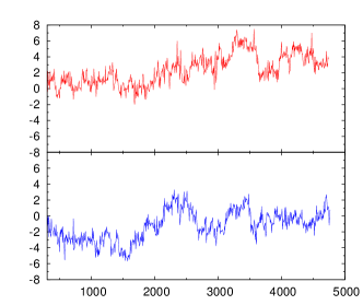
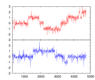
The topological charge history gives an indication of the ergodicity of the molecular dynamics evolution. Ideally, we want a reasonably good coverage of the most probable topological charge sectors. This occurs when tunneling between the topological charge sectors is reasonably frequent. It is expected that the tunneling rate decreases as the lattice spacing is decreased. Therefore, to test ergodicity in our molecular dynamics evolution, we look at the least favorable case, namely our finest lattices.

In our previous study we checked the evolution of the topological charge in our simulations down to lattice spacings $a=0.066$ fm, and found that it fluctuated quite rapidly Bazavov et al. (2012a). In the present study the lattice spacing for our two finest lattices corresponding to $\beta=7.596$ and $\beta=7.825$ is smaller still, namely, $a=0.049$ fm and $0.041$ fm, respectively. In Fig. 12 we show the evolution of the topological charge for those two ensembles. The figures show a slower tunneling rate than in our previous study, but we still see a reasonable coverage of the topological charge sectors.

Figure 12: The evolution of topological charge in Monte-Carlo time for $\beta=7.596$ (left) and $\beta=7.825$ (right). The top and bottom panels correspond to two different streams for hybrid Monte-Carlo evolution.

Appendix B Lattice scale

To translate lattice observables to physical dimensionfull quantities, we need to measure the lattice spacing. We consider three methods for determining the scale: the static-quark-potential parameters $r_{1}$ or $r_{0}$, the gradient flow parameter $w_{0}$ Borsanyi et al. (2012b), and the kaon decay constant $f_{K}$. Our preferred method uses the static quark potential. The other methods are used as a cross check. We discuss here the the former three ways to set the scale and defer the discussion of $f_{K}$ to Appendix C.

B.1 Static quark potential

The static quark potential is used indirectly to set the scale. In brief, a standard radius $r_{0}$ Sommer (1994) or $r_{1}$ Bernard et al. (2005) is calculated from the measured heavy quark potential using Eqs. (1) and (2). On any ensemble, the standard radii are first determined in lattice units: $r_{0}/a$ and $r_{1}/a$. The values of $r_{0}$ and $r_{1}$ in the continuum limit are known in physical units from other lattice studies, based on, for example, the experimental value of $f_{\pi}$. From them and $r_{0}/a$ one can infer the value of $a$.

The static potential for the HISQ/tree action has been studied in Ref. Bazavov et al. (2012a) for a large range of gauge couplings $\beta$. We extended these studies in the following ways. We improved significantly the statistical accuracy of the calculation of the static potential at the highest beta values considered in Ref. Bazavov et al. (2012a), namely for $\beta=6.88,\leavevmode\nobreak\ 6.95,\leavevmode\nobreak\ 7.03,\leavevmode\nobreak\ 7.15$ and $7.28$. To them we added calculations of the potential at $\beta=6.740,\leavevmode\nobreak\ 7.373,\leavevmode\nobreak\ 7.596$, and $7.825$. As in our previous study, we used Coulomb gauge fixing and calculated the potential from the correlation of two Wilson lines of length $\tau$ at distance $R$. The potential is then obtained from the logarithm of the ratio of two such correlators at neighboring $\tau$ values. We fit this ratio to a constant plus a term that decays exponentially in Euclidean time $\tau$ in the interval $[\tau_{min}:\tau_{max}]$. We also studied the variation of the potential due to different choices $[\tau_{min}:\tau_{max}]$ to estimate possible systematic errors. To be specific, we used finally [2:4], [3:7], [4:9], [3:9], [4:9], [4:10], [4:10], [5:8], and [6:11] for $\beta=6.740,\leavevmode\nobreak\ 6.88,\leavevmode\nobreak\ 6.95,\leavevmode\nobreak\ 7.03,\leavevmode\nobreak\ 7.15,\leavevmode\nobreak\ 7.28,\leavevmode\nobreak\ 7.373,\leavevmode\nobreak\ 7.596$, and $7.825$, respectively.

The scales $r_{0}/a$ or $r_{1}/a$ are then determined by separately fitting the resulting potential to a Coulomb-plus-linear-plus-constant form in the $r$-intervals around the values of $r_{1}$ and $r_{0}$, respectively. We vary the fit intervals, and the variations in the extracted values of $r_{1}/a$ and $r_{0}/a$ are used as estimates of systematic errors. In most cases, the systematic errors are larger than the statistical ones. The statistical and systematic errors are added in quadrature to estimate the total error for $r_{0}$ and $r_{1}$. The values $r_{0}/a$, $r_{1}/a$ and their ratios $r_{0}/r_{1}$ determined in this study as well as from Ref. Bazavov et al. (2012a) are given in Table 4. As in our previous study, the ratio $r_{0}/r_{1}$ appears to be independent of $\beta$ (lattice spacing) within the estimated errors Bazavov et al. (2012a). Accordingly, as before, we fit the values of $r_{0}/r_{1}$ given in Table 4 to a constant for $\beta\geq 6.423$ and obtain

$$(r_{0}/r_{1})_{cont}=1.5092\pm 0.0039,\leavevmode\nobreak\ \chi^{2}/{\rm dof}=0.22\;.$$ (24)

This value agrees well with our previous estimate $r_{0}/r_{1}=1.508(5)$ Bazavov et al. (2012a). We also fit the ratio $r_{0}/r_{1}$ using only the data for $\beta\geq 6.664$ and $\beta\geq 6.608$, obtaining $r_{0}/r_{1}=1.5083(44)$ and $r_{0}/r_{1}=1.5075(43)$ with similar $\chi^{2}/{\rm dof}$. These values agree well with the one given in Eq. (24). Therefore we use Eq. (24) as our final estimate for $r_{0}/r_{1}$.

$\beta$	$r_{0}/a$	$r_{1}/a$	$r_{0}/r_{1}$
5.900	1.909(11)	1.230(133)	1.552(168)
6.000	2.094(21)	1.386(80)	1.511(89)
6.050	2.194(22)	1.440(31)	1.524(36)
6.100	2.289(21)	1.522(30)	1.504(33)
6.195	2.531(24)	1.670(30)	1.516(31)
6.285	2.750(30)	1.822(30)	1.509(30)
6.341	2.939(11)	1.935(30)	1.519(24)
6.354	2.986(41)	1.959(30)	1.524(31)
6.423	3.189(22)	2.096(21)	1.522(18)
6.460	3.282(32)	2.165(20)	1.516(20)
6.488	3.395(31)	2.235(21)	1.519(20)
6.550	3.585(14)	2.369(21)	1.513(15)
6.608	3.774(20)	2.518(21)	1.499(15)
6.664	3.994(14)	2.644(23)	1.511(14)
6.740	4.293(32)	2.856(11)	1.503(13)
6.800	4.541(30)	3.025(22)	1.501(15)
6.880	4.959(28)	3.265(23)	1.519(14)
6.950	5.249(20)	3.485(22)	1.506(11)
7.030	5.691(32)	3.763(13)	1.512(10)
7.150	6.299(59)	4.212(42)	1.495(20)
7.280	7.140(53)	4.720(33)	1.513(15)
7.373	7.801(79)	5.172(34)	1.508(18)
7.596	9.443(237)	6.336(56)	1.490(40)
7.825	11.51(378)	7.690(58)	1.497(50)

Table 4: Values of $r_{1}$ and $r_{0}$ in lattice units for different $\beta$

To determine the lattice spacing as function of $\beta$, we fit $a/r_{1}$ to the Allton-type ansatz Allton (1997),

$$\displaystyle\frac{a}{r_{1}}=\frac{c_{0}f(\beta)+c_{2}(10/\beta)f^{3}(\beta)}{1+d_{2}(10/\beta)f^{2}(\beta)}\;,$$ (25)

$$\displaystyle f(\beta)=\left(\frac{10b_{0}}{\beta}\right)^{-b_{1}/(2b_{0}^{2})}\exp(-\beta/(20b_{0}))\;.$$ (26)

Here $b_{0}$ and $b_{1}$ are the well-known coefficients of the two-loop beta function, which for the three-flavor case are $b_{0}=9/(16\pi^{2})$, $b_{1}=1/(4\pi^{4})$. At small $\beta$, the parameter $r_{1}$ is small in lattice units. Therefore, to avoid possibly large discretization effects, for $\beta<6.423$, where $r_{0}/a$ is more reliably determined, we use $r_{1}/a=r_{0}/a/(r_{0}/r_{1})_{cont}$ with $(r_{0}/r_{1})_{cont}$ from Eq. (24) (see discussions in Ref. Bazavov et al. (2012a)). The fit gives $\chi^{2}/{\rm dof}=0.25$ and

$$c_{0}=43.1\pm 0.3\;,$$ (27)

$$c_{2}=343236\pm 41191\;,$$ (28)

$$d_{2}=5514\pm 755\;.$$ (29)

The errors on the above fit parameters have also been estimated using the bootstrap method which gives very similar results. The differences between the above parametrization of $r_{1}/a$ and the previous one from Ref. Bazavov et al. (2012a) are less than $0.2\%$ for $\beta<6.8$. For larger beta values the differences are larger but do not exceed $1.3\%$. To convert all quantities to physical units, as in Ref. Bazavov et al. (2012a), we use the value $r_{1}=0.3106$ fm from Bazavov et al. (2010a).

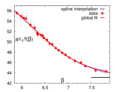
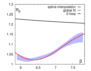
To test the uncertainty in the scale parametrization, we also fit the data for $a/r_{1}$ to the asymptotic form $f(\beta)$ times a smoothing spline. The smoothing spline is determined by minimizing the $\chi^{2}$ plus the integral of the square of the second derivative of the fit function in the considered interval times a real parameter $sm$. We chose the largest possible value of the smoothing parameter $sm=0.7$ that still gives an acceptable $\chi^{2}/{\rm dof}=1.13$. To estimate the uncertainties of the spline, we performed a bootstrap analysis. In Fig. 13, we show the $r_{1}$ scale as a function of $\beta$, normalized by the asymptotic two-loop beta function $f(\beta)$. The errors are bootstrap errors. The Allton-type fit and the smoothing spline fits give very similar results as well as uncertainties.

To calculate the EoS, we also need the nonperturbative beta function

$$R_{\beta}=-a\frac{d\beta}{da}=\frac{r_{1}}{a}\left(\frac{d(r_{1}/a)}{d\beta}\right)^{-1}\;.$$ (30)

Figure 13 shows $R_{\beta}$ obtained from both the Allton-type and smoothing-spline fits, together with bootstrap errors. The fit and the splines agree within the errors. The largest error in $R_{\beta}$ is about 3%. At sufficiently large $\beta$, i.e., close to the continuum limit, $R_{\beta}$ is expected to be given by its asymptotic two-loop form

$$R_{\beta}^{2-{\rm loop}}=20b_{0}+200b_{1}/\beta.$$ (31)

The asymptotic limit is approached from below Cheng et al. (2008), as with the p4 action. However, for the HISQ action, we see that the deviations are at most $20\%$ over the range considered, compared with a factor of two deviation in the case of the p4 action Cheng et al. (2008). In our calculations of the EoS we use $R_{\beta}$ obtained from the fit with the Allton-type ansatz.

Figure 13: The scale $a/r_{1}$ normalized by the asymptotic two-loop beta function (top) and the nonperturbative beta function, $R_{\beta}$, (bottom) as a function of $\beta$, which has been derived from this using Eq. (30); the fit and spline interpolations are also shown.

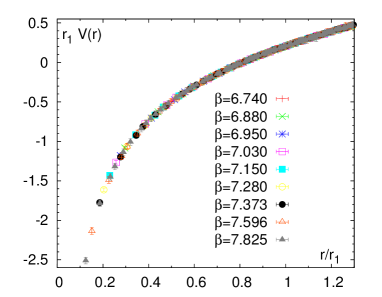
Finally, we compare the potential calculated at different $\beta$. To do so, we normalize it with an additive constant. We do this by requiring that the potential $V(r_{1})=0.2060/r_{1}$. This normalization condition is equivalent to the one used in Ref. Bazavov et al. (2012a). Here we choose $r_{1}$, because it has smaller errors on fine lattices. The normalized potential in units of $r_{1}$ is plotted in Fig. 14 against the tree-level improvement radius $r\rightarrow r_{I}$, where $r_{I}$ is the improved distance defined from the free lattice gluon propagator Bazavov et al. (2012a). Down to distances $r=0.2r_{1}$ or $r=0.062$fm, we find no significant dependence on the lattice spacing within the estimated errors.

Figure 14: The static potential versus distance in units of $r_{1}$ for different $\beta$. Here we use the improved estimator $r_{I}$ to define the distance $r$.

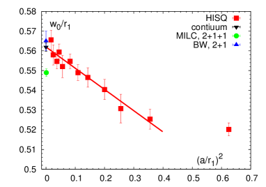
To cross check our determination of the lattice spacing, we also calculated the scale $w_{0}$, defined from the gradient flow Borsanyi et al. (2012b). Our results for the $w_{0}$ scale are shown in Fig. 15 in units of $r_{1}$. As above, for $\beta<6.423$ the value of $r_{1}$ was estimated as $r_{0}/(r_{0}/r_{1})_{cont}$. As one can see from the figure, this ratio appears to scale as $a^{2}$ for $(a/r_{1})^{2}<0.4$, i.e., for $\beta\geq 6.195$. We perform a continuum extrapolation of the ratio $w_{0}/r_{1}$ using a simple form $(w_{0}/r_{1})_{cont}+h_{w}(a/r_{1})^{2}$. In the continuum limit, we obtain $(w_{0}/r_{1})_{cont}=0.5619(21)$ or $w_{0}=0.1749(14)$ fm. This value agrees with the value quoted in Ref. Borsanyi et al. (2012b), $w_{0}=0.1755(18)(4)$ fm, within the estimated errors. Our value of $w_{0}$ is higher than the preliminary value reported by MILC $w_{0}=0.1711(2)(8)(2)(3)$fm for 2+1+1 flavor QCD Bazavov et al. (2013c). For the slope parameter we get $h_{w}=-0.1076(149)$ with $\chi^{2}/{\rm dof}=0.38$. If we use the $w_{0}$ scale instead of the $r_{1}$ scale, the temperature values for $N_{\tau}=8$ lattices for $T<150$ MeV would be lower by $6\%$, and for $N_{\tau}=10$ and $12$ calculations the differences in the temperature scale would be only $4\%$ or less.

Figure 15: The $w_{0}$ scale as function of the lattice spacing together with the continuum extrapolation. Also shown are results from 2+1 flavor QCD Borsanyi et al. (2012b) and 2+1+1 flavor QCD Bazavov et al. (2013c).

Appendix C Hadronic observables

C.1 Line of constant physics

It is standard practice to present results for thermodynamic quantities as a function of temperature at fixed, renormalized quark masses. We start by setting a constant value of the strange quark mass $m_{s}$, preferably, its physical value, and then set the mass of the light quarks to $m_{s}/20$. We determine the strange quark mass by requiring that the mass of the un-mixed pseudoscalar $s\bar{s}$ meson, $\eta_{s\bar{s}}$ is equal to a prescribed value expressed in units of $r_{1}$. We aim at the value suggested by leading order chiral perturbation theory, where the mass of $\eta_{s\bar{s}}$ meson in terms of the kaon and pion masses is, $M_{\eta_{s\bar{s}}}=\sqrt{2m_{K}^{2}-m_{\pi}^{2}}=686$ MeV. In practice, this requires some tuning and, as discussed later, it turns out that our LCP is best described by the value $M_{\eta_{s\bar{s}}}=695$ MeV. Setting the line of constant physics (LCP) in this way requires a combination of determining the lattice spacing in physical units (see Appendix B) and the hadron spectrum at zero temperature, including, at least, the mass of the $\eta_{s\bar{s}}$, a calculation with costs that mount as the lattice spacing decreases. Thus, some retuning is usually needed to correct for an imprecise determination.

For the present study, we extend the LCP of our previous work Bazavov et al. (2012a) to weaker coupling in order to cover the range needed for $N_{\tau}=12$. In our previous work, the hadron spectrum was measured along the LCP up to $\beta=6.8$. The masses of the pseudoscalar mesons were also measured at $\beta=7.28$ with the relatively low statistics of about 1,400 equilibrated time units. Here, we added or extended nine $T=0$ ensembles with $6.8<\beta\leq 7.825$ as described in Appendix B. On the extended ensembles, in addition to measuring thermodynamic quantities needed for the zero temperature subtraction, we measured the masses and decay constants of the pseudoscalar mesons and the masses of the vector mesons. These quantities allow us to quantify the lattice artifacts due to taste breaking and can be used as an alternative means to set the lattice spacing, thus providing additional validation of our calculations.

$\beta$	$aM_{\pi}$	$aM_{K}$	$aM_{\eta_{s\bar{s}}}$
5.900	0.20162(09)	0.63407(17)	0.86972(11)
6.000	0.18381(37)	0.57532(51)	0.79046(27)
6.195	0.15143(14)	0.47596(16)	0.65506(11)
6.285	0.13823(50)	0.43501(47)	0.59951(28)
6.354	0.12923(15)	0.40628(20)	0.55982(17)
6.423	0.12022(12)	0.37829(19)	0.52161(17)
6.460	0.11528(21)	0.36272(34)	0.50137(32)
6.488	0.11245(15)	0.35313(27)	0.48716(17)
6.515	0.10975(12)	0.34453(29)	0.47516(29)
6.550	0.10629(16)	0.33322(38)	0.45989(24)
6.575	0.10469(68)	0.32521(55)	0.44869(50)
6.608	0.10001(17)	0.31333(28)	0.43286(29)
6.664	0.09572(18)	0.29837(37)	0.41178(32)
6.740	0.087991(64)	0.27735(12)	0.38342(10)
6.800	0.0849(18)	0.26387(99)	0.36257(68)
6.880	0.07714(16)	0.24314(16)	0.33630(11)
7.030	0.06744(15)	0.21202(19)	0.29381(20)
7.150	0.06126(18)	0.19231(20)	0.26631(16)
7.280	0.05516(17)	0.17209(19)	0.23824(18)
7.373	0.04990(22)	0.15530(16)	0.21531(12)
7.596	0.04106(44)	0.12896(30)	0.17810(12)
7.825	0.03425(23)	0.10695(46)	0.14731(15)

Table 5: The pseudoscalar meson masses for the HISQ/tree action along the $m_{l}=0.05m_{s}$ LCP.

Figure 16: The calculated masses of the $\eta_{s\bar{s}}$ meson normalized by the chosen LCP value $M_{\eta_{s\bar{s}}}=695$ MeV as a function of $\beta$.

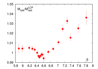
The masses of the three pseudoscalar mesons are given in lattice units in Table 5. The mass of the $\eta_{s\bar{s}}$ normalized by the value $M_{\eta_{s\bar{s}}}=695$ MeV used to define the LCP is plotted in Fig. 16 as a function of $\beta$. As one can see, the central values are systematically above the nominal value of $685.8$ MeV quoted in Ref. Davies et al. (2010). The average value from ensembles with $\beta<7.03$ is about $695$ MeV. Therefore, we define our LCP using this value. That is, we choose a strange quark mass that gives $M_{\eta_{s\bar{s}}}=695$ MeV. The resulting strange quark mass is then about $2.6\%$ larger than its physical value. For $\beta\leq 7.03$ we find that $M_{\eta_{s\bar{s}}}$ (and, in turn, the strange quark mass) along the LCP agrees with the physical values within (1–2)$\sigma$. For the finest ensembles, $\beta>7.03$, we see a systematic deviation of $M_{\eta_{s\bar{s}}}$ towards higher values — by as much as about 3.5%.

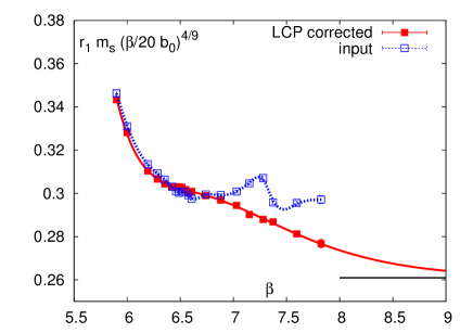
For the calculation of the trace anomaly, we need the strange quark mass $m_{s}$ and its derivative as a function of $\beta$ along the LCP. As we have seen, the strange-quark mass input into the simulation drifts slightly above the LCP. We correct for this drift using lowest order chiral perturbation theory, $i.e.$, we assume that $M_{\eta_{s\bar{s}}}^{2}$ is proportional to $m_{s}$ and calculate the strange quark mass that gives $M_{\eta_{s\bar{s}}}=695$ MeV. This corrected value is compared with the value used in the simulations in Fig. 17. For the worst case, $\beta=7.825$, this amounts to lowering $m_{s}$ used by about 7% from the simulated value. The pion and kaon masses follow a pattern similar to that of the $\eta_{s\bar{s}}$ meson, i.e., they are roughly constant for $\beta<7.03$ and increase for larger beta values by approximately the same fractional amount.

We then fit the product $r_{1}m_{s}^{LCP}$ using a renormalization-group-inspired form

$$r_{1}m_{s}^{LCP}\equiv\tilde{m}_{s}=r_{1}m^{RGI}\left(\frac{20b_{0}}{\beta}\right)^{4/9}\frac{1+m_{1}\frac{10}{\beta}f^{2}(\beta)+m_{2}(\frac{10}{\beta})^{2}f^{2}(\beta)+m_{3}\frac{10}{\beta}f^{4}(\beta)}{1+dm_{1}\frac{10}{\beta}f^{2}(\beta)}\;,$$ (32)

where $f(\beta)$ is the 2-loop beta function given by Eq. 26. For the fit parameters we get

$$m^{RGI}=0.2609\pm 0.0030,$$ (33)

$$m_{1}=35600\pm 6097,$$ (34)

$$m_{2}=-21760\pm 3202,$$ (35)

$$m_{3}=(2.67\pm 0.50)\cdot 10^{7},$$ (36)

$$dm_{1}=2420\pm 1346$$ (37)

$$\chi^{2}/{\rm dof}=0.51.$$ (38)

The resulting fit is shown in Fig. 17 together with a smoothing spline fit to the input strange-quark masses.

Figure 17: The input strange quark mass and the strange quark mass along LCP together with the respective fits shown as lines. The input quark masses have been fitted with a smooth spline. The horizontal line shows the assymptotic value.

C.2 Pseudoscalar decay constants

The decay constants of pseudoscalar mesons can be used to check the lattice scale and to estimate the cutoff effects in the $T=0$ calculations. Results for the decay constants are shown in Table 6.

$\beta$	$af_{\pi}$	$af_{K}$	$af_{\eta}$	# sources
6.000	0.11243(21)	0.13224(31)	0.15290(22)	1
6.195	0.09179(21)	0.10835(13)	0.12525(13)	1
6.285	0.08366(22)	0.09826(13)	0.11390(13)	1
6.354	0.07825(40)	0.09146(19)	0.10598(11)	1
6.423	0.07241(18)	0.08515(11)	0.09854(07)	2
6.460	0.06885(11)	0.08185(09)	0.09454(08)	4
6.515	0.06534(18)	0.07707(15)	0.08946(09)	4
6.575	0.06104(49)	0.07265(19)	0.08405(14)	2
6.740	0.052190(50)	0.061731(41)	0.071354(27)	2
6.800	0.04883(83)	0.05774(18)	0.06717(14)	1
6.880	0.045544(67)	0.053749(42)	0.062236(28)	2
7.030	0.03951(12)	0.046566(68)	0.054148(43)	2
7.150	0.03486(10)	0.041636(68)	0.048654(42)	2
7.280	0.03067(13)	0.036894(64)	0.043237(38)	2
7.373	0.02787(20)	0.033825(82)	0.039609(43)	2
7.596	0.02224(20)	0.02741(21)	0.032344(59)	2
7.825	0.01756(32)	0.022526(85)	0.026808(51)	2

Table 6: Results for decay constants of the pseudoscalar mesons in lattice units for the HISQ/tree action along the $m_{l}=0.05m_{s}$ LCP. We use the normalization in which $f_{\pi}\sim 90$ MeV. In the last column, we list the number of source points used on each configuration to increase the statistics.

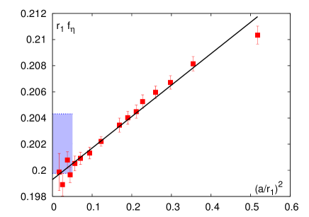
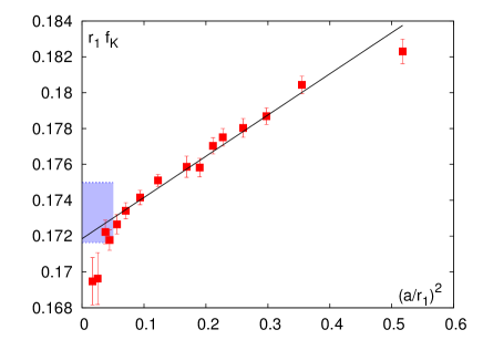
Since they are quite sensitive to the values of the quark masses, we need to take into account the deviations from the LCP, as well as the fact that even on the LCP our quark masses are slightly heavier than the physical ones. Thus, we need to interpolate/extrapolate in the quark masses. To do this we assume that the pseudoscalar decay constants depend linearly on the sum of the quark masses and use the numerical results given in Table 6 to determine the slope for each value of $\beta$. The values of the $\eta_{s\bar{s}}$ meson decay constant $f_{\eta}$ and the kaon decay constant $f_{K}$ have been interpolated to the physical quark masses using this slope. The results are shown in Fig. 18 in units of $r_{1}$. The kaon decay constant has large finite size errors at the two smallest lattices spacings. Therefore, we do not include the corresponding data in the fit. We extrapolate the values of $r_{1}f_{\eta}$ and $r_{1}f_{K}$ to zero lattice spacing assuming a simple form

$$f_{i}r_{1}=(f_{i}r_{1})^{cont}+e_{i}(a/r_{1})^{2},\leavevmode\nobreak\ \leavevmode\nobreak\ i=K,\eta.$$ (39)

For the kaon decay constant we get $(r_{1}f_{K})^{cont}=0.17186(24)$ and $e_{K}=0.0230(11)$ with $\chi^{2}/{\rm dof}=1.20$. For the $\eta_{s\bar{s}}$ decay constant we get $(r_{1}f_{\eta})^{cont}=0.19930(24)$ and $e_{\eta}=0.024(12)$ with $\chi^{2}/{\rm dof}=0.77$. The continuum extrapolation is also shown in Fig. 18, where we compare it with the value of $r_{1}f_{\eta}$ quoted in Ref. Davies et al. (2010), and find reasonable agreement. The “PDG” value plotted there is based on the PDG value of $f_{\pi}$ and the value of $f_{K}/f_{\pi}=1.194(5)$ from the recent FLAG review Aoki et al. (2013), which gives $f_{K}=155.7(9)/\sqrt{2}$ MeV. We find agreement within estimated errors.

Figure 18: The decay constants of $\eta_{s\bar{s}}$ meson (left) and kaon (right) together with the continuum extrapolations. The data are corrected for deviations from the LCP as described in the text. The bands show the value of these decay constants from Ref. Davies et al. (2010) and PDG. Here we use the value $r_{1}=0.3106(14)(8)(4)$ fm. The errors on $r_{1}$ have been added linearly and combined with the errors on $f_{\eta}$ and $f_{K}$ in quadratures.

C.3 Vector meson masses

The masses of the three vector mesons $\rho$, $K^{*}$, and $\phi$ are listed in Table 7. All three masses are adjusted to the LCP in a manner similar to the decay constants. For $\rho$ and $K^{*}$ the contribution of an excited state of the same parity is significant in the available temporal range; however, fits with an excited state typically yield low confidence levels. Therefore, in reporting masses on our finest lattices we take, as a systematic error, the difference in the fitted masses with and without an excited state of the same parity. This error is combined linearly with the statistical error in the table.

$\beta$	$aM_{\rho}$	$aM_{K^{*}}$	$aM_{\phi}$
6.195	0.7562(36)	0.8842(18)	1.0050(93)
6.354	0.6375(35)	0.7499(26)	0.8523(08)
6.423	0.6047(43)	0.6950(22)	0.7925(08)
6.460	0.5784251)	0.6709(43)	0.7644(22)
6.488	0.5647(24)	0.6478(22)	0.7363(07)
6.550	0.5324(24)	0.6118(20)	0.6929(14)
6.608	0.5072(39)	0.5757(08)	0.6523(10)
6.664	0.4732(43)	0.5501(26)	0.6180(10)
6.740	0.4286(31)	0.4996(22)	0.5732(05)
6.880	0.2828(489)	0.4359(17)	0.5000(04)
7.030	0.2937(326)	0.3750(126)	0.4333(09)
7.150	0.2866(108)	0.3387(107)	0.3901(15)
7.280	0.2535(96)	0.3026(20)	0.3467(25)
7.373	0.2363(119)	0.2774(33)	0.3165(06)
7.596	0.1923(61)	0.2272(25)	0.2593(15)
7.825	0.1543(120)	0.1884(57)	0.2140(19)

Table 7: Masses of the vector mesons in lattice units.

In Fig. 19, we show the $\phi$ meson mass $m_{\phi}$ in $r_{1}$ units as a function of the lattice spacing together with the continuum extrapolation. Again, we use the simple form $(r_{1}m_{\phi})_{cont}+g_{\phi}(a/r_{1})^{2}$ to do the continuum extrapolations, and get $(r_{1}m_{\phi})=1.5961(30)$ and $g_{\phi}=0.236(18)$ with $\chi^{2}/{\rm dof}=0.42$. Our continuum extrapolation agrees with the experimental result (shown as the band).

Figure 19: The $\phi$ meson mass as function of the lattice spacing together with the continuum extrapolation. The data are corrected for deviations from the LCP as described in the text. The band shows the experimental value.

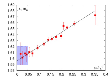
In summary, as one can see from Figs. 18 and 19, the hadronic observables provide additional valuable cross-checks for the determination of the lattice spacing. The cutoff dependence of $f_{K}$ and $m_{\phi}$ is very similar to the cutoff dependence of $w_{0}$. Therefore, the change in the lattice spacing and the temperature scale will be similar to the case when $w_{0}$ is used to set the lattice spacing.

Appendix D Observables for EoS

In this appendix, we summarize the quantities we used to evaluate the trace anomaly. They include the expectation values of local observables such as the gauge action density $s_{G}$ and the light and strange quark condensates. At nonzero temperature, we also report results for the disconnected light and strange chiral susceptibilities ($\chi_{l}^{disc}$ and $\chi_{s}^{disc}$), i.e., the fluctuations of the light and strange quark condensates, as well as the bare Polyakov loop $L_{bare}$. We use the same definitions of these quantities as in Ref. Bazavov et al. (2012a). In particular, the quark condensates are normalized per single flavor, the disconnected chiral susceptibility for light quarks is normalized for two flavors, and the disconnected chiral susceptibility for strange quarks is normalized for a single flavor.

The gauge action density and the quark condensates for zero temperature are given in Table 8. The observables at nonzero temperature are summarized in Tables 9, 10, 11, and 12 for $N_{\tau}=6,\leavevmode\nobreak\ 8,\leavevmode\nobreak\ 10$, and $12$ lattices.

For the calculation of the trace anomaly, one also needs the lattice spacing in units of $r_{1}$, the nonperturbative beta function $R_{\beta}$, the strange quark mass as function of $\beta$ along the LCP and the mass renormalization function $R_{m}$ calculated along the LCP. The parametrization of $r_{1}/a$ and $R_{\beta}$ and the calculation of their errors have been discussed in Appendix B. In Table 8, we give these quantities with their errors. The value of $m_{s}$ along the LCP has been discussed in Appendix C, where an explicit parametrization of $\tilde{m}_{s}=r_{1}m_{s}^{LCP}$ has been given. The mass renormalization function $R_{m}$ can be written as

$$R_{m}=-R_{\beta}^{-1}(1-\tilde{R}_{m}R_{\beta}),\quad\tilde{R}_{m}=\frac{1}{\tilde{m}_{s}}\frac{d\tilde{m}_{s}}{d\beta}.$$ (40)

The values of $\tilde{m}_{s}$ and $\tilde{R}_{m}R_{\beta}$ are also given in Table 8. As one can see from Figs. 16 and 17, the deviations of the input strange quark masses from the LCP for $\beta\geq 7.03$ are at most $7\%$ and are below $1\%$ for $\beta<7.03$. To include the errors arising from the deviations from the LCP, we assign a 1% error to $m_{s}$ for $\beta<7.03$ and 10% errors to $m_{s}$ for $\beta\geq 7.03$ in Eq. (9). All the errors discussed above are added in quadratures to get the the total error estimate of the trace anomaly presented in Sec. III. Our estimate of the systematic errors on the trace anomaly due to the deviations from LCP includes only the difference between the input $m_{s}$ and the value of $m_{s}$ along the LCP. Since $m_{l}/m_{s}$ is kept constant, there is no additional uncertainty due to $m_{l}$. The value of $m_{s}$, however, will affect the expectation value of the gluon action and the quark condensates shown in Eqs.(8,9). We did not estimate these effects, but based on the past experience Bernard et al. (2007); Cheng et al. (2010) we expect that these will be small.

$\beta$	$\langle s_{G}\rangle$	$\langle\bar{\psi}\psi\rangle_{l}$	$\langle\bar{\psi}\psi\rangle_{s}$	$r_{1}/a$	$R_{\beta}$	$\tilde{m}_{s}$	$R_{\beta}R_{m}$
5.900	2.632783(101)	0.049104(40)	0.105812(26)	1.264( 5)	1.048(17)	0.16563(166)	-1.6999(114)
5.950	2.597143(81)	0.043881(54)	0.098036(32)	1.325( 5)	1.043(17)	0.16060(161)	-1.5925(97)
6.000	2.561602(72)	0.038908(37)	0.090108(26)	1.390( 4)	1.038(16)	0.15646(156)	-1.4972(77)
6.025	2.544156(82)	0.036579(45)	0.086515(29)	1.424( 4)	1.036(15)	0.15468(155)	-1.4545(66)
6.050	2.526767(19)	0.034355(45)	0.083052(30)	1.459( 4)	1.034(15)	0.15306(153)	-1.4149(60)
6.075	2.509536(128)	0.032248(36)	0.079962(31)	1.494( 4)	1.032(14)	0.15160(152)	-1.3783(51)
6.100	2.492425(78)	0.030236(36)	0.076478(23)	1.531( 4)	1.030(14)	0.15028(150)	-1.3448(47)
6.125	2.475464(21)	0.028340(18)	0.073315(10)	1.568( 4)	1.028(13)	0.14908(149)	-1.3141(40)
6.150	2.458696(42)	0.026433(38)	0.070257(16)	1.607( 4)	1.027(13)	0.14799(148)	-1.2866(36)
6.175	2.442094(39)	0.024793(20)	0.067305(13)	1.646( 4)	1.025(12)	0.14701(147)	-1.2614(31)
6.195	2.429035(30)	0.023470(19)	0.064892(12)	1.679( 4)	1.025(12)	0.14629(146)	-1.2435(29)
6.245	2.396804(11)	0.020449(14)	0.059664(10)	1.762( 4)	1.023(10)	0.14470(145)	-1.2049(20)
6.285	2.3716826(153)	0.0183176(150)	0.0557043(69)	1.833( 4)	1.022( 9)	0.14362(144)	-1.1803(16)
6.341	2.3374387(197)	0.0156426(187)	0.0506613(102)	1.936( 4)	1.021( 8)	0.14231(142)	-1.1538(12)
6.354	2.3297339(226)	0.0151142(157)	0.0495513(82)	1.961( 4)	1.021( 8)	0.14204(142)	-1.1489(12)
6.390	2.3084526(343)	0.0135987(151)	0.0464432(90)	2.031( 4)	1.021( 8)	0.14133(141)	-1.1373(11)
6.423	2.2894362(269)	0.0124345(110)	0.0440691(80)	2.098( 5)	1.022( 8)	0.14072(141)	-1.1292(10)
6.460	2.2685484(184)	0.0111926(157)	0.0413543(72)	2.175( 5)	1.022( 8)	0.14008(140)	-1.1223(10)
6.488	2.2530949(69)	0.0103368(80)	0.0395263(45)	2.235( 5)	1.023( 9)	0.13962(140)	-1.1186(10)
6.515	2.2384913(119)	0.0096409(162)	0.0379912(95)	2.295( 5)	1.024( 9)	0.13919(139)	-1.1160(10)
6.550	2.2198533(261)	0.0087186(96)	0.0359905(69)	2.375( 5)	1.026(10)	0.13864(139)	-1.1141(11)
6.575	2.2068224(107)	0.0081675(80)	0.0345257(68)	2.434( 5)	1.027(10)	0.13826(138)	-1.1134(11)
6.608	2.1899477(85)	0.0074639(60)	0.0327412(57)	2.513( 5)	1.029(10)	0.13776(138)	-1.1134(11)
6.664	2.1620782(110)	0.0064352(101)	0.0302931(50)	2.654( 5)	1.033(10)	0.13691(137)	-1.1150(11)
6.740	2.1257817(133)	0.0053945(96)	0.0272312(48)	2.856( 5)	1.039(10)	0.13574(136)	-1.1196(12)
6.800	2.0982834(130)	0.0045273(53)	0.0250900(34)	3.026( 6)	1.045(10)	0.13479(135)	-1.1244(12)
6.880	2.0630924(76)	0.0038178(57)	0.0224907(35)	3.266( 7)	1.053(10)	0.13348(133)	-1.1313(12)
6.950	2.0336080(100)	0.0030671(68)	0.0206297(36)	3.491( 7)	1.061(10)	0.13230(132)	-1.1373(13)
7.030	2.0012582(67)	0.0027057(50)	0.0186364(23)	3.764( 8)	1.071(10)	0.13091(1309)	-1.1435(13)
7.150	1.9552310(112)	0.0021015(39)	0.0162827(22)	4.209(11)	1.085(11)	0.12878(1288)	-1.1507(15)
7.280	1.9083452(117)	0.0015991(68)	0.0140717(28)	4.743(13)	1.101(11)	0.12646(1265)	-1.1552(16)
7.373	1.8765238(46)	0.0012932(102)	0.0122227(24)	5.160(15)	1.112(12)	0.12481(1248)	-1.1562(17)
7.596	1.8053831(35)	0.0008701(71)	0.0095488(14)	6.297(24)	1.135(21)	0.12103(1210)	-1.1524(28)
7.825	1.7388070(42)	0.0005625(54)	0.0075428(23)	7.696(51)	1.154(27)	0.11751(1175)	-1.1420(33)

Table 8: The gauge action density, light and strange quark condensates at zero temperatures. Also shown are the values of $r_{1}/a$, $\tilde{m}_{s}$, $R_{\beta}$ and $R_{\beta}R_{m}$ used in the calculation of the trace anomaly along the LCP.

$\beta$	$T$ [MeV]	$\langle s_{G}\rangle$	$\langle\bar{\psi}\psi\rangle_{l}$	$\langle\bar{\psi}\psi\rangle_{s}$	$\chi^{disc}_{l}$	$\chi^{disc}_{s}$	$L_{bare}$
5.900	133.8	2.632253(64)	0.044948(25)	0.105106(15)	0.577(10)	0.0644(17)	0.002599(20)
5.950	140.3	2.596445(58)	0.038962(28)	0.097108(17)	0.655(12)	0.0681(19)	0.003157(22)
6.000	147.2	2.560827(68)	0.032932(30)	0.088920(16)	0.741(11)	0.0704(14)	0.004077(20)
6.025	150.8	2.543240(18)	0.029995(27)	0.085152(10)	0.810(16)	0.0711(15)	0.004600(32)
6.050	154.5	2.525666(19)	0.027029(32)	0.081458(18)	0.946(26)	0.0754(27)	0.005294(33)
6.075	158.2	2.508305(33)	0.024144(50)	0.078122(26)	1.061(19)	0.0777(21)	0.006013(28)
6.100	162.1	2.490962(34)	0.020983(31)	0.074290(16)	1.148(23)	0.0798(18)	0.007027(18)
6.125	166.0	2.473804(31)	0.017975(47)	0.070757(17)	1.223(24)	0.0816(29)	0.008156(31)
6.150	170.1	2.456840(33)	0.014837(53)	0.067264(24)	1.313(28)	0.0889(19)	0.009463(53)
6.175	174.3	2.439980(29)	0.012008(39)	0.063819(18)	1.148(26)	0.0906(31)	0.010942(55)
6.195	177.8	2.426644(30)	0.009958(46)	0.061004(18)	1.009(22)	0.0932(15)	0.012192(42)
6.245	186.5	2.394214(29)	0.006302(37)	0.054910(31)	0.440(12)	0.0866(23)	0.015619(71)
6.285	194.1	2.368816(49)	0.004572(23)	0.050296(23)	0.1963(71)	0.0753(28)	0.018535(49)
6.341	205.0	2.334602(54)	0.003229(14)	0.044690(24)	0.0686(34)	0.0724(20)	0.022822(75)
6.354	207.6	2.326948(71)	0.0030128(68)	0.043460(18)	0.05033(157)	0.06293(215)	0.023805(68)
6.423	222.1	2.286667(62)	0.0022268(37)	0.037597(16)	0.01467(44)	0.04245(122)	0.029564(72)
6.488	236.6	2.250583(43)	0.0018235(37)	0.033135(14)	0.00656(46)	0.02796(45)	0.034892(104)
6.515	243.0	2.236043(44)	0.0017067(23)	0.031671(12)	0.00394(25)	0.02268(48)	0.037358(81)
6.550	251.4	2.217540(36)	0.0015783(23)	0.029853(10)	0.00289(28)	0.01663(45)	0.040428(102)
6.575	257.7	2.204590(57)	0.0014903(19)	0.028517(10)	0.00186(20)	0.01368(46)	0.042698(84)
6.608	266.1	2.187842(66)	0.0013966(12)	0.026962( 8)	0.00166(13)	0.01048(32)	0.045373(81)
6.664	281.0	2.160154(56)	0.00127253(92)	0.0249128(67)	0.000646(55)	0.006665(202)	0.050566(88)
6.800	320.4	2.096708(55)	0.00104636(41)	0.0207485(33)	0.000170(48)	0.002140(77)	0.062640(66)
6.950	369.6	2.032442(34)	0.00086791(28)	0.0172826(20)	0.000055(14)	0.000795(36)	0.076417(96)
7.150	445.6	1.954433(30)	0.000696540(50)	0.01390563(83)	0.00000214(44)	0.0002043(52)	0.094300(69)
7.280	502.1	1.907706(57)	0.000609280(48)	0.01216886(50)	0.00000388(166)	0.0001201(108)	0.105861(91)
7.373	546.3	1.875942(38)	0.000531641(23)	0.01062292(55)	0.000001297(43)	0.0002442(32)	0.113932(98)
7.596	666.7	1.805019(28)	0.000422615(31)	0.00844724(40)	0.000001080(397)	0.0001474(113)	0.132910(111)
7.825	814.8	1.738571(16)	0.000338793(10)	0.00677357(19)	0.0000003877(22)	0.00007679(64)	0.151621(112)

Table 9: Expectation value of local observables calculated on $N_{\tau}=6$ lattices

$\beta$	$T$ [MeV]	$\langle s_{G}\rangle$	$\langle\bar{\psi}\psi\rangle_{l}$	$\langle\bar{\psi}\psi\rangle_{s}$	$\chi^{disc}_{l}$	$\chi^{disc}_{s}$	$L_{bare}$
6.050	115.8	2.5266237(348)	0.0327762(186)	0.0828810(115)	0.4139(69)	0.05669(150)	0.0004353(134)
6.125	124.5	2.4753158(262)	0.0264181(110)	0.0730705(82)	0.4706(75)	0.06081(109)	0.0006204(47)
6.175	130.7	2.4419268(287)	0.0225733(227)	0.0669802(122)	0.4779(81)	0.05382(134)	0.0008371(116)
6.195	133.3	2.4288377(376)	0.0211403(154)	0.0645320(91)	0.4973(132)	0.05412(245)	0.0009414(166)
6.245	139.9	2.3965418(294)	0.0177511(150)	0.0591829(61)	0.5346(109)	0.05172(93)	0.0012420(117)
6.285	145.5	2.3713746(283)	0.0151984(242)	0.0550896(84)	0.5607(334)	0.04938(161)	0.0016083(177)
6.341	153.7	2.3370256(418)	0.0118052(185)	0.0498389(77)	0.7507(139)	0.05228(141)	0.0022252(131)
6.354	155.7	2.3292352(137)	0.0109211(513)	0.0485851(197)	0.8123(357)	0.05624(304)	0.0024708(325)
6.390	161.3	2.3079034(111)	0.0088051(453)	0.0452635(142)	0.8915(238)	0.05593(184)	0.0031329(387)
6.423	166.6	2.2887805(179)	0.0069624(573)	0.0426307(216)	0.9083(238)	0.05822(342)	0.0038408(355)
6.460	172.7	2.2678076(214)	0.0050971(363)	0.0395899(152)	0.6520(254)	0.05707(351)	0.0048401(370)
6.488	177.5	2.2523061(146)	0.0040973(324)	0.0375676(211)	0.4791(204)	0.05586(308)	0.0055937(523)
6.515	182.2	2.2376344(146)	0.0033605(111)	0.0358104(81)	0.3208(65)	0.05421(204)	0.0064548(245)
6.550	188.6	2.2189982(111)	0.0026714(70)	0.0335964(50)	0.1676(32)	0.04600(150)	0.0076062(174)
6.575	193.3	2.2059639(144)	0.0023153(61)	0.0319944(50)	0.1061(20)	0.04065(91)	0.0084632(181)
6.608	199.5	2.1890447(95)	0.0019665(55)	0.0300405(69)	0.0554(18)	0.03770(106)	0.0096959(240)
6.664	210.7	2.1612301(160)	0.00161467(242)	0.0274505(65)	0.02910(72)	0.028704(850)	0.0118668(196)
6.740	226.8	2.1249421(157)	0.00132194(152)	0.0243573(47)	0.01123(37)	0.017709(487)	0.0150425(309)
6.800	240.3	2.0975154(118)	0.00117166(80)	0.0223027(32)	0.00606(20)	0.010758(192)	0.0176361(287)
6.880	259.3	2.0624169(93)	0.00102161(56)	0.0199079(30)	0.00282(16)	0.005774(105)	0.0213349(344)
6.950	277.2	2.0329709(115)	0.00092680(48)	0.0182584(25)	0.00138(13)	0.003370(64)	0.0246964(418)
7.030	298.9	2.0006938(123)	0.00083316(37)	0.0165135(12)	0.00080(21)	0.001763(20)	0.0286964(278)
7.150	334.2	1.9547446(127)	0.00072858(127)	0.014507068(795)	0.0001447(228)	0.0007811(177)	0.0349571(493)
7.280	376.6	1.9079588(118)	0.00063333(87)	0.012635689(523)	0.0000317(121)	0.0003433(117)	0.0419502(385)
7.373	409.7	1.8762085(84)	0.00055109(22)	0.011005082(305)	0.0000075(24)	0.0004985(47)	0.0470148(330)
7.596	500.0	1.8051472(106)	0.00043608(17)	0.008714430(192)	0.0000040(28)	0.0002289(36)	0.0595132(289)
7.825	611.1	1.73864086(834)	0.0003485897(29)	0.006968632(67)	0.000000600( 3)	0.00011855(51)	0.0725663(201)

Table 10: Expectation value of local observables calculated on $N_{\tau}=8$ lattices

$\beta$	$T$ [MeV]	$\langle s_{G}\rangle$	$\langle\bar{\psi}\psi\rangle_{l}$	$\langle\bar{\psi}\psi\rangle_{s}$	$\chi^{disc}_{l}$	$\chi^{disc}_{s}$	$L_{bare}$
6.488	142.0	2.2529939(94)	0.008717(66)	0.0392107(30)	0.4696(80)	0.03671(59)	0.0006332(54)
6.515	145.8	2.2383351(92)	0.007845(53)	0.0376092(21)	0.4983(48)	0.03601(67)	0.0007530(46)
6.575	154.6	2.2066486(87)	0.005916(112)	0.0339874(45)	0.6199(111)	0.03566(87)	0.0011236(72)
6.608	159.6	2.1897092(97)	0.004863(141)	0.0320595(57)	0.6914(140)	0.03790(54)	0.0014074(111)
6.664	168.6	2.1618075(67)	0.003366(119)	0.0293881(48)	0.5971(104)	0.03805(76)	0.0020061(99)
6.740	181.4	2.1254552(49)	0.002058(44)	0.0260341(30)	0.2350(27)	0.03178(63)	0.0030709(50)
6.800	192.2	2.0979463(46)	0.001551(21)	0.0237258(22)	0.10175(85)	0.02664(27)	0.0040471(52)
6.880	207.5	2.0627661(47)	0.001196(11)	0.0210031(13)	0.03805(50)	0.01794(15)	0.0055452(50)
6.950	221.8	2.0332765(52)	0.0010256(87)	0.0191246(19)	0.01785(44)	0.01182(21)	0.0069963(116)
7.030	239.1	2.0009567(52)	0.0008889(70)	0.0171719(16)	0.00732(49)	0.00655(12)	0.0088725(130)
7.150	267.4	1.9549570(41)	0.0007594(33)	0.01496641(85)	0.002826(227)	0.002693(65)	0.0118853(116)
7.280	301.3	1.9081112(43)	0.0006518(22)	0.01296143(67)	0.000578(120)	0.001005(28)	0.0155783(205)
7.373	327.8	1.8763272(51)	0.0005648(11)	0.01125795(32)	0.000239(83)	0.000522(29)	0.0183751(154)
7.596	400.0	1.8052323(39)	0.00044450(86)	0.008876950(228)	0.0000210(201)	0.0001413(88)	0.0256495(265)
7.825	488.9	1.7387004(82)	0.00035425( 5)	0.007080600(105)	0.00000040(14)	0.0000461(10)	0.0337466(261)

Table 11: Expectation value of local observables calculated on $N_{\tau}=10$ lattices

$\beta$	$T$ [MeV]	$\langle s_{G}\rangle$	$\langle\bar{\psi}\psi\rangle_{l}$	$\langle\bar{\psi}\psi\rangle_{s}$	$\chi^{disc}_{l}$	$\chi^{disc}_{s}$	$L_{bare}$
6.740	151.2	2.1257086(54)	0.004079(97)	0.0269239(25)	0.4498(119)	0.02317(53)	0.0004772(73)
6.800	160.2	2.0981866(76)	0.003016(120)	0.0246617(30)	0.5714(211)	0.02569(175)	0.0007167(44)
6.880	172.9	2.0629734(44)	0.001882(75)	0.0218834(45)	0.3838(75)	0.02479(102)	0.0011690(73)
6.950	184.8	2.0334633(59)	0.001339(52)	0.0198904(40)	0.1644(30)	0.02098(123)	0.0016813(86)
7.030	199.2	2.0011122(72)	0.001025(22)	0.0177901(23)	0.0617(15)	0.01489(61)	0.0024077(75)
7.150	222.8	1.9550761(46)	0.000808(10)	0.0153880(17)	0.0183(10)	0.00823(55)	0.0037030(71)
7.280	251.1	1.9082143(37)	0.000675(13)	0.0132415(21)	0.0061(12)	0.00312(13)	0.0054060(154)
7.373	273.1	1.8764082(49)	0.0005792(88)	0.01146391(89)	0.0042(12)	0.002445(51)	0.0068171(125)
7.596	333.3	1.8052889(42)	0.00045065(76)	0.00899511(28)	0.000093(58)	0.000682(11)	0.0106861(146)
7.825	407.4	1.7387435(49)	0.000358140(90)	0.00715650(16)	0.000000601(50)	0.0001120(91)	0.0153196(362)

Table 12: Expectation value of local observables calculated on $N_{\tau}=12$ lattices

References

- Wilson (1974) K. G. Wilson, Phys. Rev. D10, 2445 (1974).
- Creutz (1980) M. Creutz, Phys.Rev. D21, 2308 (1980).
- Engels et al. (1981) J. Engels, F. Karsch, H. Satz, and I. Montvay, Phys. Lett. B101, 89 (1981).
- Aoki et al. (2009) Y. Aoki, S. Borsanyi, S. Durr, Z. Fodor, S. D. Katz, et al., JHEP 0906, 088 (2009), eprint 0903.4155.
- Bazavov et al. (2012a) A. Bazavov, T. Bhattacharya, M. Cheng, C. DeTar, H. Ding, et al., Phys. Rev. D85, 054503 (2012a), eprint 1111.1710.
- Borsanyi et al. (2012a) S. Borsanyi, Z. Fodor, S. D. Katz, S. Krieg, C. Ratti, et al., JHEP 1201, 138 (2012a), eprint 1112.4416.
- Bazavov et al. (2012b) A. Bazavov et al. (HotQCD Collaboration), Phys.Rev. D86, 034509 (2012b), eprint 1203.0784.
- Bazavov et al. (2014) A. Bazavov, H. T. Ding, P. Hegde, O. Kaczmarek, F. Karsch, et al. (2014), eprint 1404.6511.
- Petreczky (2012a) P. Petreczky, J. Phys. G39, 093002 (2012a), eprint 1203.5320.
- Philipsen (2013) O. Philipsen, Prog. Part. Nucl. Phys. 70, 55 (2013), eprint 1207.5999.
- DeTar and Heller (2009) C. DeTar and U. Heller, Eur.Phys.J. A41, 405 (2009), eprint 0905.2949.
- Linde (1980) A. D. Linde, Phys. Lett. B96, 289 (1980).
- Braun-Munzinger et al. (2003) P. Braun-Munzinger, K. Redlich, and J. Stachel (2003), to appear in Quark Gluon Plasma 3, eds. R.C. Hwa and Xin-Nian Wang, World Scientific Publishing, eprint nucl-th/0304013.
- Ejiri et al. (2006) S. Ejiri, F. Karsch, and K. Redlich, Phys.Lett. B633, 275 (2006), eprint hep-ph/0509051.
- Gale et al. (2013) C. Gale, S. Jeon, and B. Schenke, Int.J.Mod.Phys. A28, 1340011 (2013), eprint 1301.5893.
- Umeda et al. (2012) T. Umeda et al. (WHOT-QCD Collaboration), Phys.Rev. D85, 094508 (2012), eprint 1202.4719.
- Heller et al. (1999) U. M. Heller, F. Karsch, and B. Sturm, Phys. Rev. D60, 114502 (1999), eprint hep-lat/9901010.
- Blum et al. (1997) T. Blum, C. E. Detar, S. A. Gottlieb, K. Rummukainen, U. M. Heller, et al., Phys. Rev. D55, 1133 (1997), eprint hep-lat/9609036.
- Orginos et al. (1999) K. Orginos, D. Toussaint, and R. Sugar (MILC Collaboration), Phys. Rev. D60, 054503 (1999), eprint hep-lat/9903032.
- Karsch et al. (2000) F. Karsch, E. Laermann, and A. Peikert, Phys. Lett. B478, 447 (2000), eprint hep-lat/0002003.
- Bernard et al. (2007) C. Bernard, T. Burch, C. E. DeTar, S. Gottlieb, L. Levkova, et al., Phys. Rev. D75, 094505 (2007), eprint hep-lat/0611031.
- Cheng et al. (2008) M. Cheng, N. Christ, S. Datta, J. van der Heide, C. Jung, et al., Phys. Rev. D77, 014511 (2008), eprint 0710.0354.
- Bazavov et al. (2009) A. Bazavov, T. Bhattacharya, M. Cheng, N. Christ, C. DeTar, et al., Phys. Rev. D80, 014504 (2009), eprint 0903.4379.
- Cheng et al. (2010) M. Cheng, S. Ejiri, P. Hegde, F. Karsch, O. Kaczmarek, et al., Phys. Rev. D81, 054504 (2010), eprint 0911.2215.
- Borsanyi et al. (2010a) S. Borsanyi, G. Endrodi, Z. Fodor, A. Jakovac, S. D. Katz, et al., JHEP 1011, 077 (2010a), eprint 1007.2580.
- Borsanyi et al. (2014) S. Borsanyi, Z. Fodor, C. Hoelbling, S. D. Katz, S. Krieg, et al., Phys.Lett. B370, 99 (2014), eprint 1309.5258.
- Follana et al. (2007) E. Follana et al. (HPQCD Collaboration, UKQCD Collaboration), Phys. Rev. D75, 054502 (2007), eprint hep-lat/0610092.
- Bazavov and Petreczky (2013a) A. Bazavov and P. Petreczky, Phys.Rev. D87, 094505 (2013a), eprint 1301.3943.
- Cea et al. (2014) P. Cea, L. Cosmai, and A. Papa (2014), eprint 1403.0821.
- Bazavov et al. (2012c) A. Bazavov, H. Ding, P. Hegde, O. Kaczmarek, F. Karsch, et al., Phys. Rev. Lett. 109, 192302 (2012c), eprint 1208.1220.
- Bazavov et al. (2013a) A. Bazavov, H. T. Ding, P. Hegde, O. Kaczmarek, F. Karsch, et al., Phys. Rev. Lett. 111, 082301 (2013a), eprint 1304.7220.
- Bazavov et al. (2013b) A. Bazavov, H. T. Ding, P. Hegde, F. Karsch, C. Miao, et al. (2013b), eprint 1309.2317.
- Bazavov and Petreczky (2013b) A. Bazavov and P. Petreczky, Eur.Phys.J. A49, 85 (2013b), eprint 1303.5500.
- Kim et al. (2013) S. Kim, P. Petreczky, and A. Rothkopf (2013), eprint 1310.6461.
- Petreczky (2012b) P. Petreczky (HotQCD Collaboration), PoS LATTICE2012, 069 (2012b), eprint 1211.1678.
- Bazavov (2013) A. Bazavov (HotQCD Collaboration), Nucl.Phys.A904-905 2013, 877c (2013), eprint 1210.6312.
- Bazavov and Petreczky (2010) A. Bazavov and P. Petreczky (HotQCD collaboration), J. Phys. Conf. Ser. 230, 012014 (2010), eprint 1005.1131.
- Sommer (1994) R. Sommer, Nucl. Phys. B411, 839 (1994), eprint hep-lat/9310022.
- Bernard et al. (2005) C. Bernard et al. (MILC Collaboration), Phys. Rev. D71, 034504 (2005), eprint hep-lat/0405029.
- Bazavov et al. (2010a) A. Bazavov et al. (MILC Collaboration), PoS LATTICE2010, 074 (2010a), eprint 1012.0868.
- Borsanyi et al. (2012b) S. Borsanyi, S. Durr, Z. Fodor, C. Hoelbling, S. D. Katz, et al., JHEP 1209, 010 (2012b), eprint 1203.4469.
- Petreczky (2009) P. Petreczky, Nucl. Phys. A830, 11C (2009), eprint 0908.1917.
- Karsch et al. (2003) F. Karsch, K. Redlich, and A. Tawfik, Eur. Phys. J. C29, 549 (2003), dedicated to Rolf Hagedorn, eprint hep-ph/0303108.
- Cheng et al. (2009) M. Cheng, P. Hendge, C. Jung, F. Karsch, O. Kaczmarek, et al., Phys. Rev. D79, 074505 (2009), eprint 0811.1006.
- Huovinen and Petreczky (2010) P. Huovinen and P. Petreczky, Nucl. Phys. A837, 26 (2010), eprint 0912.2541.
- Borsanyi et al. (2010b) S. Borsanyi et al. (Wuppertal-Budapest Collaboration), JHEP 1009, 073 (2010b), eprint 1005.3508.
- Beringer et al. (2012) J. Beringer et al. (Particle Data Group), Phys.Rev. D86, 010001 (2012).
- R Core Team (2013) R Core Team, R: A Language and Environment for Statistical Computing (Vienna, Austria, 2013), URL http://www.R-project.org/.
- Venables and Ripley (2002) W. N. Venables and B. D. Ripley, Modern Applied Statistics with S (Springer, New York, 2002), 4th ed., iSBN 0-387-95457-0, URL http://www.stats.ox.ac.uk/pub/MASS4.
- Jr et al. (2014) F. E. H. Jr, with contributions from Charles Dupont, and many others., Hmisc: Harrell Miscellaneous (2014), r package version 3.14-4, URL http://CRAN.R-project.org/package=Hmisc.
- Hung and Shuryak (1995) C. Hung and E. V. Shuryak, Phys.Rev.Lett. 75, 4003 (1995), eprint hep-ph/9412360.
- Engels and Karsch (2012) J. Engels and F. Karsch, Phys. Rev. D85, 094506 (2012), eprint 1105.0584.
- Haque et al. (2014) N. Haque, A. Bandyopadhyay, J. O. Andersen, M. G. Mustafa, M. Strickland, et al., JHEP 1405, 027 (2014), eprint 1402.6907.
- Laine and Schroder (2006) M. Laine and Y. Schroder, Phys.Rev. D73, 085009 (2006), eprint hep-ph/0603048.
- Clark et al. (2005) M. Clark, A. Kennedy, and Z. Sroczynski, Nucl. Phys. Proc. Suppl. 140, 835 (2005), eprint hep-lat/0409133.
- Hasenbusch (2001) M. Hasenbusch, Phys.Lett. B519, 177 (2001), eprint hep-lat/0107019.
- Bazavov et al. (2010b) A. Bazavov et al. (MILC collaboration), Phys. Rev. D82, 074501 (2010b), eprint 1004.0342.
- Allton (1997) C. R. Allton, Nucl.Phys.Proc.Suppl. 53, 867 (1997), eprint hep-lat/9610014.
- Bazavov et al. (2013c) A. Bazavov et al. (The MILC Collaboration) (2013c), eprint 1311.1474.
- Davies et al. (2010) C. Davies, E. Follana, I. Kendall, G. Lepage, and C. McNeile (HPQCD Collaboration), Phys. Rev. D81, 034506 (2010), eprint 0910.1229.
- Aoki et al. (2013) S. Aoki, Y. Aoki, C. Bernard, T. Blum, G. Colangelo, et al. (2013), eprint 1310.8555.