Automatic discovery of cell types and microcircuitry from neural connectomics

Abstract

Neural connectomics has begun producing massive amounts of data, necessitating new analysis methods to discover the biological and computational structure. It has long been assumed that discovering neuron types and their relation to microcircuitry is crucial to understanding neural function. Here we developed a nonparametric Bayesian technique that identifies neuron types and microcircuitry patterns in connectomics data. It combines the information traditionally used by biologists, including connectivity, cell body location and the spatial distribution of synapses, in a principled and probabilistically-coherent manner. We show that the approach recovers known neuron types in the retina and enables predictions of connectivity, better than simpler algorithms. It also can reveal interesting structure in the nervous system of C. elegans, and automatically discovers the structure of a microprocessor. Our approach extracts structural meaning from connectomics, enabling new approaches of automatically deriving anatomical insights from these emerging datasets.

1. Electrical Engineering and Computer Science, University of California, Berkeley

2. Department of Physical Medicine and Rehabilitation, Northwestern University and Rehabilitation Institute of Chicago, Chicago, Illinois

3. Department of Physiology, Northwestern University, Chicago, Illinois

4. Department of Applied Mathematics, Northwestern University, Chicago, Illinois

Introduction

Emerging connectomics techniques [1, 2] promise to quantify the location and connectivity of each neuron within a tissue volume. These massive datasets will far exceed the capacity of neuroanatomists to manually trace small circuits, thus necessitating computational, quantitative, and automatic methods for understanding neural circuit structure. The impact of this kind of high-throughput transition has been seen before – rise of sequencing techniques necessitated the development of novel computational methods to understand genomic structure, ushering in bioinformatics as an independent discipline [3].

The brain consists of multiple kinds of neurons, each of which is hypothesized to have a specific role in the overall computation. Neuron types differ in many ways, e.g. chemical or morphological, but they also differ in the way they connect to one another. In fact, the idea of well defined, type-dependent local connectivity patterns (microcircuits) has been prominent in many areas, from sensory (e.g. retina, [4] to processing (e.g. neocortex [5]) to movement (e.g. spinal cord) [6]. These sorts of repeated computing patterns are a common feature of computing systems, even arising in human-made computing circuits. It remains an important challenge to develop algorithms to use anatomical data, e.g. connectomics, to automatically back out underlying microcircuitry.

The discovery of structure is a crucial aspect of network science. Early approaches focused on global graph properties, such as the types of scaling present in the network [7]. While this approach leads to an understanding of the global network, more recent work aims at identifying very small-scale repeat patterns, or “motifs” in networks[8]. These motifs are defined not between different node types, but rather represent repeated patterns of topology.

The discovery of structure in probabilistic graphs is a well-known problem in machine learning. Commonly used algorithms include community-based-detection methods [9], and stochastic block models [10]. While these approaches can incorporate the probabilistic nature of neural connections [11] they do not incorporate the additional richer structure present in connectomics data – the location of cell bodies, the spatial distribution of synapses, and the distances between neurons. Of particular importance is that the probability of connections has a strong spatial component, a factor that is hard to reconcile with many other methods. A model attempting to fully capture the variation in the nervous system should take into account the broad set of available features.

When it comes to neuroscience and other computing systems, we expect patterns of connectivity much more complex than traditional motifs, exhibiting a strong spatial dependence arising from the complex genetic, chemical, and activity-based neural development processes.

To address these challenges, here we describe a Bayesian nonparametric model that can discover circuit structure automatically from connectomics data: the cell types, their spatial patterns of interconnection, and the locations of somata and synapses. We show that by incorporating this additional information, our model both accurately predicts the connection as well as agrees with human neuroanatomists as to the identification of cell types.

We primarily focus on the recently-released mouse retina connectome [12], but additionally examine the C. elegans connectome [13], and then “connectome” of a classical microprocessor [14]. Comparing the cell types discovered by the algorithms with those obtained manually by human anatomists reveals a high degree of agreement. We thus present a scalable probabilistic approach to infer microcircuitry from connectomics data available today and in the future.

Figure 1: Deriving circuitry and types from connectomics data a. As input we take the connectivity betwen cells (b), the distance between them (c), the depth of the cell bodies (d), and the depth profile of the syanpses (e). f. Our algorithm discovers hidden cell types in this connectivity data by assuming all cells of a type share a distance-dependent connectivity profile, similar depth, and a similar synpatic density profile, with cells of other types. This results in a clustering of the cells by those hidden types. f.) shows the cell connectivity matrix with cells of the same type grouped together. g.) shows the learned probability of connection between our different types at various distances – in this case, the cells are likely to connect when they are close. h. shows the probability of connection between two cell types that very rarely connect – there’s a background “base” connection rate to account for errors in data, but the probability is very low. We can plot this these types (i) to show the relationship and spatial connections, and how probable various types are to connect to one another. j.) The connectivity between our discovered types changes as a function of distance.

Results

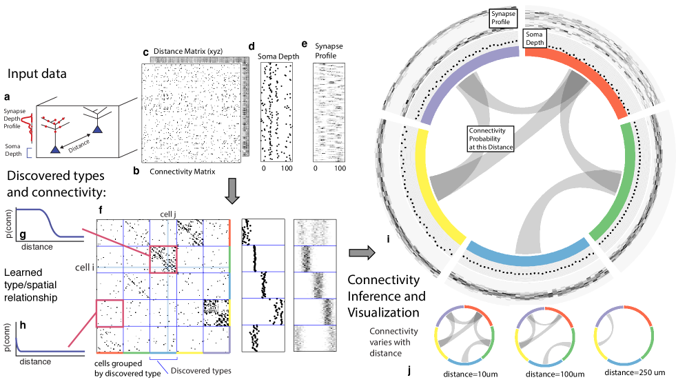
We build a structured probabilistic model which begins with the generic notion of a cell being a member of a single, unobserved type – and these types affect soma depth, distribution of synapses, as well as a cell type and distance dependent connection probability. For example, retinal ganglion cells may synapse on nearby, but not far away, amacrine cells, with ganglion cells being superficial and having a broad distribution of synapses.

From these assumptions (priors) we develop a generative Bayesian model that estimates the underlying cell types and how they connect. We take as input (fig  1a) the connectivity matrix of cells (fig  1b) , a matrix of the distance between cells (fig  1c), the per-cell soma depth (fig  1d) and the depth profile of the cell’s synapses (fig  1e). We perform joint probabilistic inference to automatically learn the number of cell types, which cells belong to which type, their type-specific connectivity, and how connections between types vary with distance. We also simultaneously learn the soma depth associated with each type and the typical synaptic density profile (fig  1f-h.).

We apply our algorithm to datasets from mouse retina, C. elegans and a historical microprocessor. Anatomists classify cells based on many features, giving us a meaningful baseline to compare against.

We start with a model for connectivity, the infinite stochastic block model (iSBM)[15, 16], which has been shown to meaningfully cluster connection graphs while learning the number of hidden groups, or types. We extend this approach by adding distance dependence to model salient aspects of microcircuitry via logistic and exponential distance-link functions. We additionally model cell body depth unimodally and synapse density profile multimodially (see Methods for mathematical details).

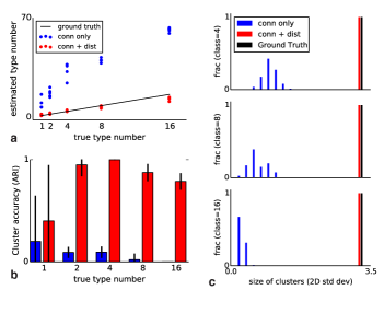
To validate our model, we performed a series of simulations to test if the model can accurately recover the true underlying network structure and cell type identity. We thus simulate data for which we know the correct structure and comparing the estimated structure based on the algorithm (see methods) with the one we used for simulation. We find that the model does a good job of recovering the correct number of cell types, (fig 2a), the the cell identities (fig 2b), and the spatial extent of each type (fig 2c). For comparison, existing infinite stochastic block model assumes cell type alone matters, and thus finds small neighborhoods of connected nodes (instead of global connectivity patterns). The model converges relatively quickly to an estimate of the most probable values for the cell types, which is enabled by using a combination of simulated annealing and parallelized Markov chain Monte Carlo (see methods for details). Thus we can apply our model to simulated datasets with structure and scale similar to that of our biological datasets and recover the known correct structure.

Figure 2: Correct recovery of true numbers of hidden types in synthetic data when incorporating spatial information. a.) The infinite stochastic block model (which only uses connectivity information) over-estimates the number of classes as it fails to take distance into account, whereas our modeling of the combination of distance and connectivity finds close to the true number of classes. b.) ARI, a measure of “correct clustering”, for different true class counts, between our model and a traditional iSBM. c.) For synthetic data, type discovery based only on connectivity are tiny spatially-localized groups – in contrast, our model recovers the true spatial extent of the underlying types.

Learning types and circuitry in the retina

Figure 3: Discovering cell classes in the mouse retina connectome. a.) Input connectivity data for 950 cells for which soma positions were known. b. clustered connectivity matrix. c.) connectivity diagram showing our clusters, as well as the cell depth and anatomist-labeled cell type of each cell. Our model shows moderate agreement with the cell types traditionally identified by anatomist laminar-specific connectivity patterns. d.) Connectivity between our clusters as a function of distance – the cluster consisting primarily of retinal ganglion cells (lower left-center) exhibits the expected near and far connectivity. e.) The spatial distribution of our cell types – each cell type tesselates space.

The mouse retina [4] is a neural circuit which we expect to have connectivity patterns that are well approximated by our generative model. It is known that there are multiple classes of cells that can be broadly grouped into: ganglion cells that transmit information to the rest of the brain, bipolar cells that connect between different cells, and amacrine cells that feed into the ganglion cells. Recent research [12] has produced a large dataset containing both the types of cells from orthogonal approaches, and also the connectivity matrix between all reconstructed cells.

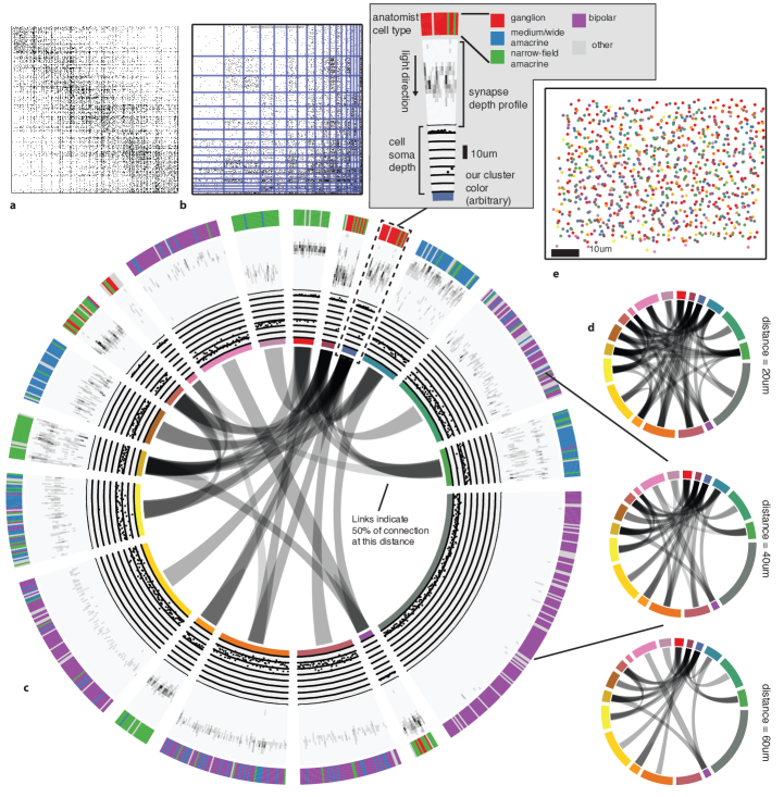
The algorithm took less than 2 hours to perform inference, dividing neurons into a set of cell types (fig 3c, each wedge is a type). For each pair of neurons there is a specific distance dependent connection probability (fig 3b,c,d), which is well approximated by the model fit. Moreover, each type of cell is rather isotropically distributed across space (fig 3e) as should be expected for true cell types.

Comparing the results of the algorithm to other information sources allows evaluating the quality of the type determination. Our types closely reflect the (anatomist-determined) segmentation of cells into retinal ganglion, narrow amacrine, medium/wide amacrine, and bipolar cells (fig 3c, outermost ring). We find that the types we find tend to reflect the known laminar distribution in the retina (fig 3c, middle ring).

The algorithm yields a separation of neurons into a smaller number of types than the fully granular listing of 71 types found by the original authors of the paper, although is still highly correlated with those finer type distinctions (see supp Mouse Retina. It is our expectation that, with larger datasets, even closer agreement would be found.

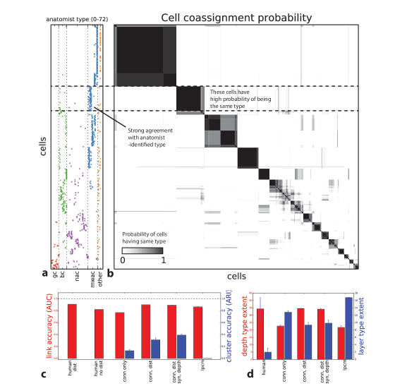
Our fully Bayesian model produces a distribution over probable clusterings. Figure 4 shows this posterior distribution as a cell-cell coassignment matrix, sorted to find maximum block structure. Each large, dark block represents a collection of cells believed with strong probability to be of the same type. When we plot (fig 4b) the anatomist-derived cell types along the left, we can see that each block consists of a roughly-homogeneous collection of types.

We evaluate our model along three sets of parameters (Fig.4): how closely does our clustering agree with neuroanatomists’ knowledge? Given two cells, how accurately can our model predict the link between them? And how closely does the spatial extent (within a layer) of our identified types agree with the known neuroanatomists.

As a first measure we compare link prediction accuracy across the methods (Fig.4 B AUC, red). We find that given the dataset many techniques allow for good link-predictive accuracy. All the methods allow decent link prediction with an AUC in the .9 range. However, our algorithm clearly outperforms the simple statistical models that only use connectivity.

As a second measure we compare link prediction accuracy across the methods (Fig.4 B ARI, blue). We find that our algorithm far outperforms the controls. We also find that when it is based on more of the same information used by anatomists use then it gets better at agreeing with these anatomists. In particular, using connectivity, distance, synapse distribution and soma depth leads to the highest ARI. When using the available information the algorithm produces a good fit to human anatomist judgments.

Finally we look at the spatial extent of the discovered types both within a layer and between layers (Fig.4 C). We see that, in the absence of distance information, mere connectivity information results in types which only span a small region of space – essentially “local cliques”. Incorporation of distance information results in types which span the entire extent of the layer. The depth variance of all models continues to be substantially larger than that predicted by human anatomists – future directions of work include attempting to more strongly encode this prior belief of laminarity.

Figure 4: Visualizing type inference uncertainty. Our fully Bayesian model gives a confidence estimate (posterior probability) that any two given cells are of the same type. In b.) we visualize that cell-cell coassignment matrix, showing the probability that cell i is of the same type as cell j on a range from 0.0 to 1.0. The block structure shows subsets of cells which are believed to all belong to the same type. For comparison, a.) shows the anatomist-defined type for each cell, grouped broadly into the coarse types identified in the previous figure. Link vs cluster accuracy c. A comparison of the predictive accuracy (area under the curve) for hand-labeled anatomical data, versus inclusion of additional sources of information, as well as the clustering accuracy. Note that our model sacrifies very little predictive accuracy for additional clustering accuracy. By comparison, conventional methods fail at one or both. d. ) The spatial extent (in depth and area) of the types identified by humans and our various algorithmic approaches.

Recovering spatial connectivity in multiple graphs simultaneously

Having shown our model to work on the repeating tessellated, laminar structure of the mammilian retina, we then apply our model to a structurally very different connectome – the whole body of a small roundworm: Caenorhabditis elegans is a model system in developmental neuroscience[13], with the location and connectivity of each of 302 neurons developmentally determined, leading to early measurement of the connectome. Unlike the retina, only the motor neurons in C. elegans exhibit regular distribution in space – along the body axis. Most interneurons are concentrated in various ganglia that project throughout the entire animal, and the sensory neurons are primarily located in a small number of anterior ganglia. C. elegans also differs from the retina in that the measured connectome is actually two separate graphs – one of directed chemical synapses and another of undirected electrical synapses.

Figure 5: Discovering connectivity and type in C. elegans. a.) Initial C. elegans cell connectivity matrix, red are (directional) chemical synapses, blue are electrical synapses. Point size is proportional to synapse count between those cells. b.) Clustered adjacency matrix showing identified clusters. c.) Inter-cluster connectivity, showing the position of each cell along the body axis as well as the “true” cell type – both coarse (motor, sensory, and interneuron) as well as fine (small text labels).

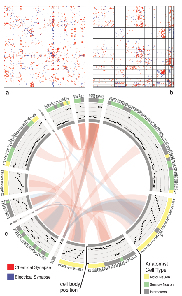
Using both the chemical and electrical connectivity (see methods), we determined the underlying clusters explained by connectivity and distance (fig 5a). A superficial inspection of the results shows clustering into groups consisting roughly homogeneously of motor neurons, sensory neurons, and interneurons. Closer examination reveals agreement with the classifications originally outlined by White in 1986.

We identify cell types that reflect the known motor/non-motor neuron classes, even though this system lacks the strong repeat microcircuitry our model was designed for. Motor-neuron types AS, DA, and VA, all exclusively postsynaptic, are identified as a common type, as are motor-neuron types VD and DD. Traditional types VC, DB, and VB also mostly share a cluster. Various head motor neurons, including types SMD and RMD, are clustered together. Interneurons with known anatomically-distinct connectivity patterns, such as AVA (2 cells), are clustered into pure types.The algorithm even correctly places the single-cell types DVB and DVC by themselves.

Note our clustering does not perfectly reflect known divisions – several combinations of head and sensory neurons are combined, and a difficult-to-explain group of mostly VB and DB motor neuron types, with VC split between various groups. Our identified cell types thus reflect a “coarsening” of known types, based entirely on connectivity and distance information, even when the organism exhibits substantially less spatial regularity than the retina.

Types and connectivity in artificial structures

Figure 6: Discovering connectivity and type the 6502 microprocessor. a.) is the micrograph of the original microprocessor, with the region containing the registers under study highlighted. b.) Our graph consists of the interconnections of MOS field-effect transistors with three terminals, Gate, C1, and C2. Reconstruction technique did not permit resolution of C1 and C2 into source and drain. c.) The spatial distribution of the transistors in each cluster show a clear pattern d.) The clusters and connectivity versus distance for connections between Gate and C1, Gate and C2, and C1 and C2 terminals on a transistor. Red and teal types have a terminal pulled down to ground and mostly function as inverters. Purple class are clocked, stateful transistors, orange control the ALU and yellow control the special data bus (SDB).

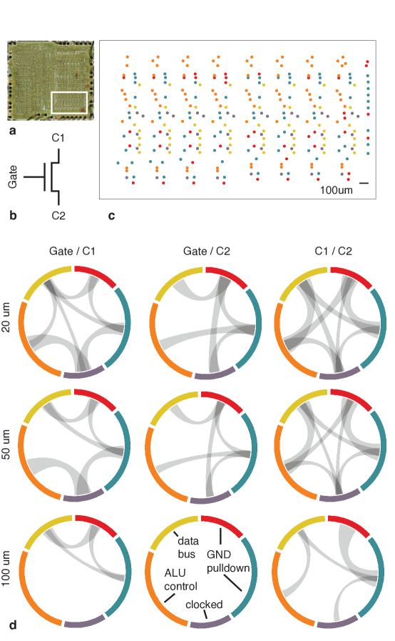
To show the applicability of our method to other connectome-style datasets, we obtained the spatial location and interconnectivity of the transistors in a classic microprocessor, the MOS Technology 6502 (used in the Apple II) [14]. Computer architects use common patterns of transistors when designing circuits, with each transistor having a “type” in the circuit. We identified a region of the processor with complex but known structure containing the primary 8-bit registers X, Y, and S (fig 6).

Our algorithm identifies areas of spatial homogeneity that mirror the known structure in the underlying architectural circuit, segmenting transistor types recognizable to computer architects. Using the original schematics, we see that one identified type contains the “clocked” transistors, which retain digital state. Two other types contain transistors with pins C1 or C2 connected to ground, mostly serving as inverters. An additional identified type controls the behavior of the three registers of interest (X, Y, and S) with respect to the SB data bus, either allowing them to latch or drive data from the bus. The repeat patterns of spatial connectivity are visible in figure 6c, showing the man-made horizontal and vertical layout of the same types of transistors.

Discussion

We have presented a machine learning technique that allows cell types and microcircuitry to be discovered from connectomics data. We have shown its applicability to regularly structured laminar neural circuits like the retina, as well as a less structured whole neuronal organism (C. elegans) and an artificial processor. When compared to existing methods, we show how the incorporation of all of this data yields results that combine both high link-prediction accuracy and high agreement with human anatomists. We have found that combining the available data types allows us to discover cell types and microcircuitry that were known to exist in the systems based on decades of previous research and allows good prediction of connectivity.

For our probabilistic models, no known solution exists to exactly find the most probable parsing of the neurons into cell-types and connectivity patterns. We employ a collection of Markov-chain Monte carlo techniques (see Methods) but while different initializations converge to similar ultimate values, we can never realistically obtain the global optimum. There are a broad range of techniques that may offer good approximations to the global optimum and future work could adapt them to find more precise solutions to our problem.

For our probabilistic model, inference becomes slower as the amount of data increases. Our algorithm required several hours for 1000 neurons. Scaling this class of probabilistic model is an active area of research, and recent results in both variational methods [17] and spectral learning [18] and future work could adapte them to find faster approximate solutions to our problem.

Larger datasets will allow algorithms to distinguish more distinct types and we expect closer agreement with existing anatomical knowledge as more data become available. Moreover, in general, for such problems precision increases with the size of the dataset and the cells that we have are not sufficient to statistically distinguish all the cell types known in anatomy (such as the $\sim 70$ in the retina). Still, using only connectivity and distance it is possible to meaningfully divide neurons into types.

Our small collection of hand-selected distance-dependent likelihood functions are clearly non-exhaustive, and assume monotonicity of connectivity probability – for a given class, closer cells are never less-likely to connect. This is known to be insufficient for various neural systems. Future models could incorporate a wider variety of likelihood functions, or even learn the global functional form from the data.

There exist a range of previous approaches to the discovery of neural microcircuitry[19, 20, 21, 22]. These generally involve a great deal of manual labor and ad-hoc determination of what constitutes a “type” of cell – to this day there are disagreements in the literature as to the “true” types in the mammalian retina. Much as phylogenomics has changed our understanding of animal ontologies, modern large scale data will allow the efficient unbiased discovery of cell types and circuits. The sheer amount of available data demands the introduction of algorithmic approaches.

The development of automatic identification and quantification of cell type may also provide a new computational phenotype for quantifying the effect of disease, genetic interventions, and developmentally-experienced neural activity. Our method can in principle identify neuron-types across non-connected graphs, e.g. across animals. For example, the types of neurons in one animal can be associated with the types of neurons in another animal, in the same way as this is already possible through molecular marker [23]. This could be particularly important if cell types appear that are due to properties of the stimuli and experience as opposed to just the molecular properties of cells, such as color and orientation selective types in primary visual cortex [24, 25]. This would allow comparative quantitative anatomy across animals, and aid the search for the ultimate causes of connectivity.

Our model combines connectivity, cellular, and synaptic properties, and suggests the way towards combining even richer data. Distinct cell types differ in morphology, connectivity, transcriptomics, relation to behavior or stimuli and many other ways. Algorithms combining this data and type type information may allow us to synthesize all the available information from one experiment or even across experiments into a joint model of brain structure and function.

Our work shows how rich probabilistic models can contribute to computational neuroanatomy. Eventually, algorithms will have to become a central tool for anatomists, as it will progressively become impossible for humans to parse the huge datasets. This transition may follow a similar transition to that of molecular biology (with gene-finding algorithms) and evolutionary biology with (computational phylogenetics). Ultimately, computational approaches may help resolve the significant disagreements across human anatomists.

Methods Summary

For the basic link-distance model, we take as input a connectivity matrix $R$ defining the connections between cell $e_{i}$ and $e_{j}$, as well as a distance function $d(e_{i},e_{j})$ representing a (physical) distance between adjacent cells. See the supplemental material for extension to multiple connectivity matrices. We assume there exist an unknown number $K$ of latent (unobserved) cell types, $k\in\{1,2,3,\dots,K\}$, and that each cell $e_{i}$ belongs to a single cell type. We indicate a cell $e_{i}$ is of type $k$ using the assignment vector $\mathbf{(}c)$, so $c_{i}=k$. The observed connectivity between two cells $R(e_{i},e_{j})$ then depends only on their latent type and their distance through a link function $f(\cdot,d(e_{i},e_{j}))$. We assume $f$ is parameterized based on the latent type, $c_{i}=m$ and $c_{j}=n$, via a parameter$\eta_{mn}$, as well as a set of global hyper parameters $\theta$, such that the link function is $f(d(e_{i},e_{j})|\eta_{mn},\theta)$.

We then jointly infer the maximum a posteriori (MAP) estimate of the class assignment vector $\mathbf{(}c)=\{c_{i}\}$, the parameter matrix $\eta_{mn}$, and the global model hyperparameters $\theta$ :

$$p(\mathbf{c},\eta,\theta|R)\propto\prod_{i,j}p(R(e_{i},e_{j})|f(d(e_{i},e_{j})|\eta_{c_{i}c_{j}}),\theta)\prod_{m,n}p(\eta_{mn}|\theta)p(\theta)p(\mathbf{c}|\alpha)p(\alpha)p(\theta)$$ (1)

For the retina data, we then extend the model with the additional features indicated. Cell soma depth is modeled as a cell-type-dependent Gaussian with latent (unknown) per-type mean and variance. Similarly, each cell has some number $N_{i}$ of synapses, each of which is drawn from a cell-type-specific density profile with up to three modes.

Inference is performed in three steps via composable transition kernels – one for structural, one for per-type parameters, and one kernel for global parameters and hyperparameters. Details of data preprocessing, inference parameters, and runtime can be found in the Methods section.

• Acknowledgments We thank Josh Vogelstein for discussions and reading of the manuscript, Finale Doshi-Velez for early discussions on the model, and Erica Peterson, and Jonathan Glidden, and Yarden Katz for extensive manuscript review. Funding for compute time was provided by Amazon Web Services “AWS in Education” grants.

• Author Contributions KK and EJ developed model. EJ derived inference, implemented code, tested, and ran experiments. KK and EJ wrote manuscript text and solicited feedback.

• Competing Interests The authors declare that they have no competing financial interests.

• Correspondence Correspondence and requests for materials should be addressed to E.J. (email: jonas@eecs.berkeley.edu).

Methods

Probabilistic Model

Our model is a extension of the iSBM [15, 16] to incorporate spatial relations between entities, inspired by attempts to extend these models with arbitrary discriminative functions[26].

We take as input a connectivity matrix $R$ defining the connections between cell $e_{i}$ and $e_{j}$, as well as a distance function $d(e_{i},e_{j})$ representing a (physical) distance between adjacent cells. See the supplemental material for extension to multiple connectivity matrices. We assume there exist an unknown number $K$ of latent (unobserved) cell types, $k\in\{1,2,3,\dots,K\}$, and that each cell $e_{i}$ belongs to a single cell type. We indicate a cell $e_{i}$ is of type $k$ using the assignment vector $\mathbf{(}c)$, so $c_{i}=k$. The observed connectivity between two cells $R(e_{i},e_{j})$ then depends only on their latent type and their distance through a link function $f(\cdot,d(e_{i},e_{j}))$. We assume $f$ is parameterized based on the latent type, $c_{i}=m$ and $c_{j}=n$, via a parameter$\eta_{mn}$, as well as a set of global hyper parameters $\theta$, such that the link function is $f(d(e_{i},e_{j})|\eta_{mn},\theta)$.

We then jointly infer the maximum a posteriori (MAP) estimate of the class assignment vector $\mathbf{(}c)=\{c_{i}\}$, the parameter matrix $\eta_{mn}$, and the global model hyperparameters $\theta$ :

$$p(\mathbf{c},\eta,\theta|R)\propto\prod_{i,j}p(R(e_{i},e_{j})|f(d(e_{i},e_{j})|\eta_{c_{i}c_{j}}),\theta)\prod_{m,n}p(\eta_{mn}|\theta)p(\theta)p(\mathbf{c}|\alpha)p(\alpha)p(\theta)$$ (2)

We describe the spatial “Logistic-distance Bernoulli” function here, and others in the supplemental material.

The “logistic-distance Bernoulli” spatial model assumes that, if cell $e_{i}$ is of type $m$ and cell $e_{j}$ is of type $n$, then $\eta_{mn}=(\mu_{mn},\lambda_{mn})$, and the probability that two cells $e_{i}$ and $e_{j}$ are connected is given by

$$p^{*} = \frac{1.0}{1+\exp\frac{d(e_{i},e_{j})-\mu_{mn}}{\lambda_{mn}}}$$ (3)

$$p = p^{*}\cdot(p_{max}-p_{min})+p_{min}$$ (4)

where $p_{max}$ and $p_{min}$ are global per-graph parameters.

We place an exponential priors on the latent parameters:

$$\mu_{mn}\sim\exp(\mu|\mu^{hp})$$ (5)

$$\lambda_{mn}\sim\exp(\lambda|\lambda^{hp})$$ (6)

using $\lambda^{hp}$ and $\mu^{hp}$ as global per-graph hyperparameters.

We use a Dirichlet-process prior on class assignments, which allows the number of classs to be determined automatically. In brief, for $N$ total cells, the probability of a cell belonging to a class is proportional to the number of datapoints already in that class, $N_{k}$, such that $p(c_{i}=k)\propto\frac{m_{k}}{N+\alpha}$ and the probability of the cell belonging to a new class $k^{\prime}$ is $p(c_{i}=k^{\prime})\propto\frac{\alpha}{N+\alpha}$. $\alpha$ is the global concentration parameter – larger values of $\alpha$ make the model more likely to propose new classes. We grid the parameter $\alpha$ and allow the best value to be learned from the data.

Where we model cell depth, we assume that each cell type has a typical depth, and thus a Gaussian distribution of $s_{i}$. We assume $s_{i}\sim N(\mu^{(s)}_{k},\sigma^{2(s)}_{k})$, where the $(s)$ superscript indicates these model parameters are associated with the soma-depth portion of our model. We use a conjugate prior for $(\mu^{(s)}_{k},\sigma^{2(s)}_{k})$ with $\mu^{(s)}_{k}\sim N(\mu^{(s)}_{hp},\sigma^{2(s)}_{k}/\kappa^{(s)}_{hp})$ and $\sigma^{2(s)}_{k}\sim\chi^{-1}(\sigma^{2(s)}_{hp},\nu^{(s)}_{hp}$. The use of conjugacy simplifies inference while allowing for each cell-type to have its own depth mean and distribution.

Where we model synapse depth profile, we assume that each cell type has a characteristic depth distribution of synaptic contact points, and thus a mixture of Gaussians distribution over cell $i$’s $N_{i}$ contact points, $\mathbf{g^{i}}$. We do this by assuming the $g^{i}_{j}$ are drawn from an $M=3$-component mixture of Gaussians. Thus associated with each cell type $k$ is a vector of $M$ Gaussian means $(\mu^{g}_{k,1},\cdots,\mu^{g}_{k,M})$, and a mixture vector $\pi_{k}$. This representation can thus model depth distributions of contact points that have up to three modes, an assumption that is well matched in the bulk of anatomical studies of cell-type dependent connectivity.

Inference

We perform posterior inference via Markov-chain Monte Carlo (MCMC), annealing on the global likelihood during the traditional burn-in phase. MCMC transition kernels for different parts of the state space can be chained together to construct a kernel whose ergodic distribution is the target ergodic distribution over the entire state space.

Our first transition kernel (“structural”) performs gibbs sampling of the assignment vector $p(\mathbf{c}|\eta,\theta,\alpha)$. The lack of conjugacy in our likelihood model makes an explicit evaluation of the conditional assignment probabilities impossible, motivating us to use an auxiliary variable method [27] in which a collection of ephemeral classs are explicitly represented for the duration of the Gibbs scan.

We then employ a transition kernel to update the per-component parameter values $\eta_{mn}$. Conditioned on the assignment vector $\mathbf{c}$ and the model hyperparameters $\theta,\alpha$ the individual $\eta_{mn}$ are independent. We slice sample [28] each component’s parameters, choosing the slice width as a function of the global hyperparameter range.

The global hyper-parameters, both $\alpha$ and $\theta$, are allowed to take on a discrete set of possible values. As $\theta$ is often a tuple of possible values, we explore the cartesian product of all possible values. We then Gibbs sample (our final transition kernel), which is always possible in a small, finite, discrete state space.

We chain these three kernels together, and then globally anneal on the likelihood from a temperature of $T=64$ down to $T=1$ over $900$ iterations unless otherwise indicated, and then run the chain for another $100$ iterations. We then generate at least $20$ samples, each taken from the end of a single Markov chain initialized from different random initial points in the state space. For visualization we pick the chain with the highest log likelihood, but for all numerical comparisons (including link probability and cluster accuracy) we use this full collection of samples from the posterior distribution to estimate the resulting statistics.

Link Prediction

As a proxy for link-prediction accuracy we compute the probability of a link between two cells using each model, trained fully on the data. While this method is potentially prone to overfitting, the overfitting will be shared across models and in fact will preferentially bias in favor of competing models which over-cluster the data. We use a full collection of posterior samples when computing the link probability, and then compute the area under the ROC curve for each.

Model Comparison

We compare our model with a standard network clustering model, the latent-position clustering model. This model assumes each cell belongs to one of K clusters, and each cluster is associated with a $d-$dimensional Gaussian distribution. The probability of a link is then a function of the distance between the data points in this continuous-space. We use [29] a variational implementation provided in R, parametrically varying the number of latent dimensions and the number of requested groups. While this model provides reasonable link predictive accuracy, the clusterings dramatically disagree with those from human anatomists.

Parameters

Hierarchical generative models can be sensitive to hyperparameter settings, thus for most hyperparamters we perform inference. In cases where we cannot we run separate collections of markov chains at separate settings and show the results across all pooled parameters. For the case of the mouse retina data, we consisder maximum link probability $p_{max}\in\{0.95,0.9,0.7\}$, variance scales for the synapse density profile of $\sigma^{2}\in\{0.01,0.1,1.0\}$ (of normalized depth), and $K\in\{2,3\}$ possible synapse density profile mixture components. For the connectivity-distance-only model we actually perform inference over both $p_{max}$ and $p_{min}$.

Mixing of our Markov chains

Evaluating whether or not approximate inference methods, such as MCMC, produce samples which are valid approximations of the posterior distribution is an ongoing area of research in the computational statistics community. We use a rough proxy here – synthetic likelihood evaluation. For synthetic datasets of sizes comparable to our real data size, do we recover known ground truth information after running our markov chains for the appropriate amount of time?

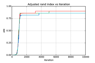
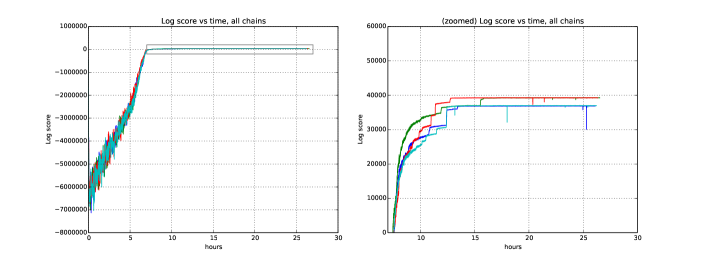
Figures 7 and 8 shows the cluster accuracy (ARI) to ground truth and the total log score as a function of runtime. We see dramatic changes in log score initially as we vary the temperature, stabilizing as runtime progresses, for each chain. Then we see the characteristic jumps between nearby modes towards the end of the run, in both log score and ARI. Importantly, regardless of whether our model over- or under-estimates the exact posterior variance about the network, we find points in the latent variable space that are both predictive and parsimonious, largely agreeing with the human anatomists and predicting existing connections.

Figure 7: Adjusted rand index for synthetic data as a function of run iteration.

Figure 8: Total model score (log score) vs iteration

Mouse Retina

Dense serial electron microscopy of a $114\mu m\times 80\mu m$ area in the mouse retina by [12] yielded a listing of places where neurons come into contact. There were over 1000 cells originally, and selected the $950$ for which the location of the soma could be reconstructed from the provided cell plots (soma locations were not provided by the study’s authors in machine-readable form). Ultimately this left a matrix between the total synapse-like contact area between all pairs of 950 cells. Area was thresholded at $0.1\mu m$, determined by hand, to yield a 950 $\times$ 950 entry matrix that served as input to our algorithm. We measured the distance between cells using the reconstructed soma centers, and used the Logistic-Distance spatial relation. Hyperprior griddings are shown in supplemental section Hyperprior grids and hyperprior inference.

C. elegans

We obtained the connectome of c. elegans from data published previously [30], and isolated the 279 nonpharyngeal neurons, with a total of 6393 chemical synapses and 890 gap junctions originally cleaned up in [31]. A cell’s position was its distance along the anterior-posterior axis normalized between zero and one. We used both networks, the chemical network as a directed graph and the electrical network as undirected graph. We use the synapse counts with the logistic-distance poisson likelihood, scaling the counts by 4.0 to compensate for the Poisson’s overdispersion.

Microprocessor

We extracted the connection graph for the transistors in the MOS6502 [32]. Each transistor has three terminals (gate, source, drain), but the methods of the original dataset were unable to consistently resolve which of the C1 and C2 terminals were source and drain, leading to ambiguity in our encoding. We identified a region consisting of three registers X, Y, and S via visual inspection and focused our efforts there. We created a total of six connectivity matrices by examining possible terminal pairings. One graph, for example, $R^{gc_{1}}(e_{i},e_{j})=1$ if transistor $e_{j}$ and $e_{j}$ are connected via pins $g$ and $c_{1}$.

Supplemental Material

Other Likelihoods

We reparameterized the Logistic-Distance Bernoulli likelihood to better capture the microprocessor data structure. We are explicitly setting the maximum probability $p$ of the logistic function on a per-component basis, drawing from a global $p\sim\operatorname{Beta}(\alpha_{hp},\beta_{hp})$. Then $\lambda$ is set for each component as a global hyperparameter, $\lambda$.

The “logstic-distance Poisson” spatial model is used to explicitly mode the count of synapses, $c$, between two neurons. The probability of c synapses between two neurons is distributed $c\sim\textrm{Poisson}(c|r)$, where $r$ (the “rate”) is generated by a scaled logistic function (the logistic function has range $[0,1]$. For each component $\eta_{mn}$ we learn both the threshold $\mu_{mn}$ and the rate scaling factor $r_{mn}$ Thus if for cells $m$ and $n$ are likely to have on average $20$ synases if they are closer than $5\mu m$, then $\mu_{mn}=5$ and $r_{mn}=20$ ”

Thus the probability of $R(e_{i},e_{j})=c$ synapses between two cells $e_{i}$ and $e_{j}$ is given by:

$$r^{*} = \frac{1.0}{1+\exp\frac{d(e_{i},e_{j})-\mu_{mn}}{\lambda}}$$ (7)

$$r = r^{*}\cdot(r_{mn}-r_{min})+r_{min}$$ (8)

$$R(e_{i},e_{j})\sim\textrm{Poisson}(c|r)$$ (9)

where $\lambda$ and $r_{min}$ are per-graph parameters. Per-component parameters $\mu_{mn}\sim\exp(\mu|\mu^{hp})$ and $r_{mn}\sim\exp(r_{mn}|r_{scale}^{hp})$.

Source code and data

All source code and materials for running experiments can be obtained from the project website, at

https://github.com/ericmjonas/netmotifs/

and the content of this paper along with scripts to run experiments and generate all figures can be found at

https://github.com/ericmjonas/connect-disco-paper/

All preprocessed data has been made publicaly available as well.

Please contact the author for pre-publication access.

Extension to multiple graphs

The model can handle multiple graphs $R^{q}$ simultaneously with a shared clustering by extending the likelihood to include the product of the likelihoods of the individual graphs.

$$p(\mathbf{c},\{\eta^{q}\},\{\theta^{q}\}|\{R^{q}\})\propto\prod_{q}\Bigg{(}\prod_{i,j}p(R^{q}(e_{i},e_{j})|f(d(e_{i},e_{j})|\eta^{q}_{c_{i}c_{j}},\theta^{q})\prod_{m,n}p(\eta^{q}_{mn}|\theta^{q})p(\theta^{q})\Bigg{)}p(\mathbf{c}|\alpha)p(\alpha)$$ (10)

Hyperprior grids and hyperprior inference

For the mouse retina Logistic-Distance Bernoulli model, we gridded $\mu^{hp}$ and $\lambda^{hp}$ into 40 $\log_{10}$-spaced points 1.0 and 80.

For the c. elegans data with the Logistic Distance poisson model, we gridded $\mu_{hp}$ and $\lambda$ into 20 $\log_{10}$-spaced points bween 0.2 and 2.0, and the $ratescale^{hp}$ parameter into 20 $\log_{10}$-spaced points between 2.0 and 20.0. We globally set $rate_{min}=0.01$.

For the microprocessor with the Logistic Distance fixed lambda Bernoulli likelihood, we gridded $mu_{hp}$ into 50 $\log_{10}$-spaced points between 10 and 500 and set $\lambda=\mu_{hp}/10$. $p_{min}\in\{0.001,0.01,0.02\}$ and both $p_{\alpha}$ and $p_{\beta}\in\{0.1,1.0,2.0\}$.

Measuring clustering similarity

The adjusted rand index (ARI) is a measure of the similarity of two different clusterings [33] – two identical clusters have an ARI of 1.0 while progressively more dissimilar clusters have lower ARIs, becoming negative as the clustering gets anti-correlated.

References

- [1] Joshua L Morgan and Jeff W Lichtman “Why not connectomics?” In Nature Methods 10.6, 2013, pp. 494–500 DOI: 10.1038/nmeth.2480
- [2] Anthony M Zador et al. “Sequencing the connectome.” In PLoS biology 10.10, 2012, pp. e1001411 DOI: 10.1371/journal.pbio.1001411
- [3] Daniel C Koboldt et al. “The next-generation sequencing revolution and its impact on genomics.” In Cell 155.1 Elsevier Inc., 2013, pp. 27–38 DOI: 10.1016/j.cell.2013.09.006
- [4] R H Masland “The fundamental plan of the retina.” In Nature neuroscience 4.9, 2001, pp. 877–86 DOI: 10.1038/nn0901-877
- [5] V B Mountcastle “The columnar organization of the neocortex.” In Brain : a journal of neurology 120 ( Pt 4, 1997, pp. 701–22 URL: http://www.ncbi.nlm.nih.gov/pubmed/9153131
- [6] Sten Grillner et al. “Microcircuits in action–from CPGs to neocortex.” In Trends in neurosciences 28.10, 2005, pp. 525–33 DOI: 10.1016/j.tins.2005.08.003
- [7] D J Watts and S H Strogatz “Collective dynamics of ’small-world’ networks.” In Nature 393.6684, 1998, pp. 440–2 DOI: 10.1038/30918
- [8] R Milo et al. “Network motifs: simple building blocks of complex networks.” In Science (New York, N.Y.) 298.5594, 2002, pp. 824–7 DOI: 10.1126/science.298.5594.824
- [9] M Girvan and M E J Newman “Community structure in social and biological networks.” In Proceedings of the National Academy of Sciences of the United States of America 99.12, 2002, pp. 7821–6 DOI: 10.1073/pnas.122653799
- [10] Krzysztof Nowicki and Tom a. Snijders “Estimation and Prediction for Stochastic Blockstructures” In Journal of the American Statistical Association 96.455, 2001, pp. 1077–1087 DOI: 10.1198/016214501753208735
- [11] Sean L Hill et al. “Statistical connectivity provides a sufficient foundation for specific functional connectivity in neocortical neural microcircuits.” In Proceedings of the National Academy of Sciences of the United States of America 109.42, 2012, pp. E2885–94 DOI: 10.1073/pnas.1202128109
- [12] Moritz Helmstaedter et al. “Connectomic reconstruction of the inner plexiform layer in the mouse retina” In Nature 500.7461 Nature Publishing Group, 2013, pp. 168–174 DOI: 10.1038/nature12346
- [13] JG White, E Southgate, JN Thomson and S BRenner “The Structure of the Nervous System of the Nematode Caenorhabditis elegans” In Philosophical transactions of the Royal Society of London. Series B, Biological sciences 314.1165, 1986, pp. 1–340
- [14] Greg James, Barry Silverman and Brian Silverman “Visualizing a classic CPU in action” In ACM SIGGRAPH 2010 Talks on - SIGGRAPH ’10 New York, New York, USA: ACM Press, 2010, pp. 1 DOI: 10.1145/1837026.1837061
- [15] Charles Kemp, JB Tenenbaum and TL Griffiths “Learning systems of concepts with an infinite relational model” In Twenty-first National Conference on Artificial Intelligence (AAAI-06), 2006 URL: http://www.aaai.org/Papers/AAAI/2006/AAAI06-061.pdf
- [16] Zhao Xu, Volker Tresp, Kai Yu and Hans-peter Kriegel “Infinite Hidden Relational Models” In Proceedings of the Twenty-Second Conference on Uncertainty in Artificial Intelligence, 2006
- [17] Matthew D Hoffman, David M Blei, Chong Wang and John Paisley “Stochastic Variational Inference” In Journal of Machine Learning Research 14, 2013, pp. 1303–1347
- [18] Anima Anandkumar et al. “Tensor Decompositions for Learning Latent Variable Models”, 2012, pp. 1–55 arXiv:arXiv:1210.7559v2
- [19] Vernon B Mountcastle “Modality and topographic properties of single neurons of cat’s somatic sensory cortex” In Journal of Neurophysiology 20, 1957, pp. 408–434 URL: http://jn.physiology.org/content/jn/20/4/408.full.pdf
- [20] RJ Douglas and KA Martin “A functional microcircuit for cat visual cortex.” In The Journal of Physiology, 1991, pp. 735–769 URL: http://jp.physoc.org/content/440/1/735.short
- [21] Peter Barthó et al. “Characterization of neocortical principal cells and interneurons by network interactions and extracellular features.” In Journal of neurophysiology 92.1, 2004, pp. 600–8 DOI: 10.1152/jn.01170.2003
- [22] T.F. Freund and G. Buzsáki “Interneurons of the hippocampus” In Hippocampus 6.4, 1998, pp. 347–470 DOI: 10.1002/(SICI)1098-1063(1996)6:4¡347::AID-HIPO1¿3.0.CO;2-I
- [23] Solange P Brown and Shaul Hestrin “Cell-type identity: a key to unlocking the function of neocortical circuits.” In Current opinion in neurobiology 19.4, 2009, pp. 415–21 DOI: 10.1016/j.conb.2009.07.011
- [24] Lawrence C Sincich and Jonathan C Horton “The circuitry of V1 and V2: integration of color, form, and motion.” In Annual review of neuroscience 28, 2005, pp. 303–26 DOI: 10.1146/annurev.neuro.28.061604.135731
- [25] Peter Lennie and J Anthony Movshon “Coding of color and form in the geniculostriate visual pathway (invited review)” In Journal of the Optical Society of America A 22.10, 2005, pp. 2013 DOI: 10.1364/JOSAA.22.002013
- [26] Kevin P Murphy “Machine Learning: A Probabilistic Perspective” Cambridge: The MIT Press, 2012
- [27] Radford M. Neal “Markov Chain Sampling Methods for Dirichlet Process Mixture Models” In Journal of Computational and Graphical Statistics 9.2, 2000, pp. 249 DOI: 10.2307/1390653
- [28] R.M. Neal “Slice sampling” In Annals of Statistics 31.3 JSTOR, 2003, pp. 705–741 DOI: 10.1214/aos/1056562461
- [29] Michael Salter-Townshend and Thomas Brendan Murphy “Variational Bayesian inference for the Latent Position Cluster Model for network data” In Computational Statistics & Data Analysis 57.1 Elsevier B.V., 2013, pp. 661–671 DOI: 10.1016/j.csda.2012.08.004
- [30] Lav R Varshney et al. “Structural properties of the Caenorhabditis elegans neuronal network.” In PLoS computational biology 7.2, 2011, pp. e1001066 DOI: 10.1371/journal.pcbi.1001066
- [31] Beth L Chen, David H Hall and Dmitri B Chklovskii “Wiring optimization can relate neuronal structure and function.” In Proceedings of the National Academy of Sciences of the United States of America 103.12, 2006, pp. 4723–8 DOI: 10.1073/pnas.0506806103
- [32] “Github: Visual6502” In 2013 URL: https://github.com/trebonian/visual6502
- [33] Lawrence Hubert and Phipps Arabie “Comparing partitions” In Journal of Classification 2.1, 1985, pp. 193–218 DOI: 10.1007/BF01908075