Structure of the third moment
of the generalized Rosenblatt distribution

Shuyang Bai  Murad Taqqu
Abstract

The Rosenblatt distribution appears as limit in non-central limit theorems. The generalized Rosenblatt distribution is obtained by allowing different power exponents in the kernel that defines the usual Rosenblatt distribution. We derive an explicit formula for its third moment, correcting the one in Maejima and Tudor (2012) and Tudor (2013). Evaluating this formula numerically, we are able to confirm that the class of generalized Hermite processes is strictly richer than the class of Hermite processes.

00footnotetext: Key words Long memory; Self-similar processes; ; Rosenblatt processes; Generalized Rosenblatt processes 2010 AMS Classification: 60G18, 60F05

1 Introduction

The Rosenblatt process is a non-Gaussian self-similar process with stationary increments. It can be represented by a double Wiener-Itô integral as follows:

Zγ(t)=A20t(sx1)+γ(sx2)+γ𝑑sB(dx1)B(dx2),subscript𝑍𝛾𝑡𝐴superscriptsubscriptsuperscript2superscriptsubscript0𝑡superscriptsubscript𝑠subscript𝑥1𝛾superscriptsubscript𝑠subscript𝑥2𝛾differential-d𝑠𝐵𝑑subscript𝑥1𝐵𝑑subscript𝑥2Z_{\gamma}(t)=A~{}\int_{\mathbb{R}^{2}}^{\prime}~{}\int_{0}^{t}(s-x_{1})_{+}^{\gamma}(s-x_{2})_{+}^{\gamma}ds~{}B(dx_{1})B(dx_{2}), (1)

where A0𝐴0A\neq 0 is a constant, the prime indicates the exclusion of the diagonals x1=x2subscript𝑥1subscript𝑥2x_{1}=x_{2} in the integral, γ(3/4,1/2)𝛾3412\gamma\in(-3/4,-1/2), and B()𝐵B(\cdot) is a Brownian random measure. The process is self-similar with Hurst index H=2γ+2(1/2,1)𝐻2𝛾2121H=2\gamma+2\in(1/2,1), that is, for any constant a>0𝑎0a>0, {Z(at)}𝑍𝑎𝑡\{Z(at)\} and {aHZ(t)}superscript𝑎𝐻𝑍𝑡\{a^{H}Z(t)\} have the same finite-dimensional distributions.

The marginal distribution of Zγ(t)subscript𝑍𝛾𝑡Z_{\gamma}(t), which we call the Rosenblatt distribution, was first characterized by Rosenblatt (1961), and the Rosenblatt process was then defined in Taqqu (1975). The Rosenblatt process belongs to a more general class of processes called Hermite processes. A k𝑘k-th order Hermite process is defined through a k𝑘k-tuple Wiener Itô integral with integrand 0tj=1k(sxj)+γdssuperscriptsubscript0𝑡superscriptsubscriptproduct𝑗1𝑘superscriptsubscript𝑠subscript𝑥𝑗𝛾𝑑𝑠\int_{0}^{t}\prod_{j=1}^{k}(s-x_{j})_{+}^{\gamma}ds in (1), where 1/21/(2k)<γ<1/21212𝑘𝛾12-1/2-1/(2k)<\gamma<-1/2. The Rosenblatt process is thus a Hermite process with k=2𝑘2k=2. Hermite processes can appear as limits in so-called non-central limit theorems involving a nonlinear function of a long-range dependent Gaussian process (Dobrushin and Major (1979), Taqqu (1979)), or a nonlinear function of a long-range dependent linear process (Surgailis (1982), Ho and Hsing (1997)).

Maejima and Tudor (2012) considered the following extension of the Rosenblatt process:

Zγ1,γ2(t)=A220t[(sx1)+γ1(sx2)+γ2+(sx1)+γ2(sx2)+γ1]𝑑sB(dx1)B(dx2),subscript𝑍subscript𝛾1subscript𝛾2𝑡𝐴2superscriptsubscriptsuperscript2superscriptsubscript0𝑡delimited-[]superscriptsubscript𝑠subscript𝑥1subscript𝛾1superscriptsubscript𝑠subscript𝑥2subscript𝛾2superscriptsubscript𝑠subscript𝑥1subscript𝛾2superscriptsubscript𝑠subscript𝑥2subscript𝛾1differential-d𝑠𝐵𝑑subscript𝑥1𝐵𝑑subscript𝑥2Z_{\gamma_{1},\gamma_{2}}(t)=\frac{A}{2}~{}\int_{\mathbb{R}^{2}}^{\prime}~{}\int_{0}^{t}[(s-x_{1})_{+}^{\gamma_{1}}(s-x_{2})_{+}^{\gamma_{2}}+(s-x_{1})_{+}^{\gamma_{2}}(s-x_{2})_{+}^{\gamma_{1}}]ds~{}B(dx_{1})B(dx_{2}), (2)

where

γ1,γ2(1,1/2) and γ1+γ2>3/2.subscript𝛾1subscript𝛾2112 and subscript𝛾1subscript𝛾232\gamma_{1},\gamma_{2}\in(-1,-1/2)\text{ and }\gamma_{1}+\gamma_{2}>-3/2.

We shall call Zγ1,γ2(t)subscript𝑍subscript𝛾1subscript𝛾2𝑡Z_{\gamma_{1},\gamma_{2}}(t) a generalized Rosenblatt process. They computed the second and the third moment of the Zγ1,γ2(1)subscript𝑍subscript𝛾1subscript𝛾21Z_{\gamma_{1},\gamma_{2}}(1), but unfortunately their formula for the third moment is incorrect. The third moment will play a crucial role in the identification of the process.

The generalized Rosenblatt process Zγ1,γ2(t)subscript𝑍subscript𝛾1subscript𝛾2𝑡Z_{\gamma_{1},\gamma_{2}}(t) belongs to a broad class of self-similar process with stationary increments defined on a Wiener chaos called generalized Hermite process, which was first introduced by Mori and Oodaira (1986). See also Bai and Taqqu (2014b) for details.

A generalized Hermite process can be represented by a multiple Wiener-Itô integral as

Zg(t)=0tg(sx1,,sxk)1{s1>x1,,sk>xk}𝑑sB(dx1)B(dxk),subscript𝑍𝑔𝑡superscriptsubscriptsuperscriptsubscript0𝑡𝑔𝑠subscript𝑥1𝑠subscript𝑥𝑘subscript1formulae-sequencesubscript𝑠1subscript𝑥1subscript𝑠𝑘subscript𝑥𝑘differential-d𝑠𝐵𝑑subscript𝑥1𝐵𝑑subscript𝑥𝑘Z_{g}(t)=\int_{\mathbb{R}}^{\prime}~{}\int_{0}^{t}g(s-x_{1},\ldots,s-x_{k})1_{\{s_{1}>x_{1},\ldots,s_{k}>x_{k}\}}ds~{}B(dx_{1})\ldots B(dx_{k}), (3)

where the nonzero function g𝑔g is called a generalized Hermite kernel (GHK) and is defined by the following two properties:

  1. 1.

    g(λx1,,λxk)=λαg(x1,,xk)𝑔𝜆subscript𝑥1𝜆subscript𝑥𝑘superscript𝜆𝛼𝑔subscript𝑥1subscript𝑥𝑘g(\lambda x_{1},\ldots,\lambda x_{k})=\lambda^{\alpha}g(x_{1},\ldots,x_{k}), for some α(k/21/2,k/2)𝛼𝑘212𝑘2\alpha\in(-k/2-1/2,-k/2);

  2. 2.

    +k|g(1+x1,,1+xk)g(x1,,xk)|𝑑𝐱<subscriptsuperscriptsubscript𝑘𝑔1subscript𝑥11subscript𝑥𝑘𝑔subscript𝑥1subscript𝑥𝑘differential-d𝐱\int_{\mathbb{R}_{+}^{k}}|g(1+x_{1},\ldots,1+x_{k})g(x_{1},\ldots,x_{k})|d\mathbf{x}<\infty.

The first condition is one of homogeneity to ensure that the resulting process Zg(t)subscript𝑍𝑔𝑡Z_{g}(t) is self-similar. The second condition ensures that the integrand in (3) is square integrable. By heuristically interchanging the order of the two integrations 0tdssuperscriptsubscript0𝑡𝑑𝑠\int_{0}^{t}\cdot ds and kB(dx1)B(dxk)superscriptsubscriptsuperscript𝑘𝐵𝑑subscript𝑥1𝐵𝑑subscript𝑥𝑘\int_{\mathbb{R}^{k}}^{\prime}\cdot B(dx_{1})\ldots B(dx_{k}) in (3), the process can be viewed as an integrated process of a stationary nonlinear moving average, which explains the stationary increments of Zg(t)subscript𝑍𝑔𝑡Z_{g}(t).

Note that for Zγ1,γ2subscript𝑍subscript𝛾1subscript𝛾2Z_{\gamma_{1},\gamma_{2}} in (2),

g(x1,x2)=A2[x1γ1x2γ2+x1γ2x2γ1],𝑔subscript𝑥1subscript𝑥2𝐴2delimited-[]superscriptsubscript𝑥1subscript𝛾1superscriptsubscript𝑥2subscript𝛾2superscriptsubscript𝑥1subscript𝛾2superscriptsubscript𝑥2subscript𝛾1g(x_{1},x_{2})=\frac{A}{2}[x_{1}^{\gamma_{1}}x_{2}^{\gamma_{2}}+x_{1}^{\gamma_{2}}x_{2}^{\gamma_{1}}],

and α=γ1+γ2𝛼subscript𝛾1subscript𝛾2\alpha=\gamma_{1}+\gamma_{2}. It follows Bai and Taqqu (2014b) that Zg(t)subscript𝑍𝑔𝑡Z_{g}(t) is self-similar with Hurst index

H=α+k/2+1(1/2,1).𝐻𝛼𝑘21121H=\alpha+k/2+1\in(1/2,1).

The process Zgsubscript𝑍𝑔Z_{g} and other related processes appear as limits in various types of non-central limit theorems involving Voterra-type nonlinear process. See Bai and Taqqu (2014c) and Bai and Taqqu (2014a) for details. The following is a natural question:

Is the class of generalized Hermite processes strictly richer than the class of Hermite processes for a given k𝑘k and H𝐻H? 111Processes differing by a multiplicative constant are considered to be the same process.

Since all generalized Hermite processes are H𝐻H-self-similar with stationary increments, they all have identical covariances up to a multiplicative factor. Hence the covariance cannot be of any help in answering the preceding question.

In this paper, we answer the preceding question positively by computing explicitly the second and the third moment of the marginal law of the generalized Rosenblatt process Zγ1,γ2(t)subscript𝑍subscript𝛾1subscript𝛾2𝑡Z_{\gamma_{1},\gamma_{2}}(t) in (2) at t=1𝑡1t=1, namely, the law of Zγ1,γ2(1)subscript𝑍subscript𝛾1subscript𝛾21Z_{\gamma_{1},\gamma_{2}}(1) which we call the generalized Rosenblatt distribution. Since the second and the third moments can be expressed in terms of beta functions, one can evaluate the moments numerically in an accurate way, and use them to show that the preceding question has a positive answer.

Remark 1.1.

The second moment formula (4) has been obtained in Lemma 2.2 of Maejima and Tudor (2012)222Maejima and Tudor (2012) also attempted to compute the third moment, but unfortunately the function fH1,H2(u1,u2,u3)subscript𝑓subscript𝐻1subscript𝐻2subscript𝑢1subscript𝑢2subscript𝑢3f_{H_{1},H_{2}}(u_{1},u_{2},u_{3}) in the proof of their Proposition 3.1 was not computed correctly. The exponents in the first and the third factor of fH1,H2(u1,u2,u3)subscript𝑓subscript𝐻1subscript𝐻2subscript𝑢1subscript𝑢2subscript𝑢3f_{H_{1},H_{2}}(u_{1},u_{2},u_{3}) should be H11subscript𝐻11H_{1}-1 and H21subscript𝐻21H_{2}-1 respectively according to their Lemma 2.1. This error was reproduced in the proof of Proposition 3.10 of Tudor (2013)..

The paper is organized as follows. In Section 2, we state our formulas for the second and the third moments of Zγ1,γ2(1)subscript𝑍subscript𝛾1subscript𝛾21Z_{\gamma_{1},\gamma_{2}}(1). Section 3 contains some preliminary lemmas. Section 4 contains the proof of the results of Section 2. In Section 5, we present the numerical evaluation of the third moment of a standardized Zγ1,γ2(1)subscript𝑍subscript𝛾1subscript𝛾21Z_{\gamma_{1},\gamma_{2}}(1) and answer positively the question stated above.

2 Main results

The random variable Zγ1,γ2(1)subscript𝑍subscript𝛾1subscript𝛾21Z_{\gamma_{1},\gamma_{2}}(1) defined in (2) has mean μ1(γ1,γ2)=0subscript𝜇1subscript𝛾1subscript𝛾20\mu_{1}(\gamma_{1},\gamma_{2})=0 since it is expressed as a Wiener-Itô integral. The following theorem provides an explicit expression of the second and the third moment of Zγ1,γ2(1)subscript𝑍subscript𝛾1subscript𝛾21Z_{\gamma_{1},\gamma_{2}}(1).

Theorem 2.1.

The second moment of Zγ1,γ2(1)subscript𝑍subscript𝛾1subscript𝛾21Z_{\gamma_{1},\gamma_{2}}(1) is

μ2(γ1,γ2)=subscript𝜇2subscript𝛾1subscript𝛾2absent\displaystyle\mu_{2}(\gamma_{1},\gamma_{2})= A2(γ1+γ2+2)(2(γ1+γ2)+3)×\displaystyle\frac{A^{2}}{(\gamma_{1}+\gamma_{2}+2)(2(\gamma_{1}+\gamma_{2})+3)}\times
[B(γ1+1,γ1γ21)B(γ2+1,γ1γ21)+B(γ1+1,2γ11)B(γ2+1,2γ21)],delimited-[]Bsubscript𝛾11subscript𝛾1subscript𝛾21Bsubscript𝛾21subscript𝛾1subscript𝛾21Bsubscript𝛾112subscript𝛾11Bsubscript𝛾212subscript𝛾21\displaystyle\big{[}\mathrm{B}(\gamma_{1}+1,-\gamma_{1}-\gamma_{2}-1)\mathrm{B}(\gamma_{2}+1,-\gamma_{1}-\gamma_{2}-1)+\mathrm{B}(\gamma_{1}+1,-2\gamma_{1}-1)\mathrm{B}(\gamma_{2}+1,-2\gamma_{2}-1)\big{]}, (4)

where B(x,y)B𝑥𝑦\mathrm{B}(x,y) denotes the beta function (6). The third moment of Zγ1,γ2(1)subscript𝑍subscript𝛾1subscript𝛾21Z_{\gamma_{1},\gamma_{2}}(1) is

μ3(γ1,γ2)=subscript𝜇3subscript𝛾1subscript𝛾2absent\displaystyle\mu_{3}(\gamma_{1},\gamma_{2})= 2A3(γ1+γ2+2)(3(γ1+γ2)+5)×\displaystyle\frac{2A^{3}}{(\gamma_{1}+\gamma_{2}+2)(3(\gamma_{1}+\gamma_{2})+5)}\times
[σ{1,2}3B(γσ1+1,γσ1γσ31)B(γσ1+1,γσ1γσ21)B(γσ2+1,γσ2γσ31)×\displaystyle\Big{[}\sum_{\sigma\in\{1,2\}^{3}}B(\gamma_{\sigma_{1}}+1,-\gamma_{\sigma_{1}}-\gamma_{\sigma_{3}^{\prime}}-1)B(\gamma_{\sigma_{1}^{\prime}}+1,-\gamma_{\sigma_{1}^{\prime}}-\gamma_{\sigma_{2}}-1)B(\gamma_{\sigma_{2}^{\prime}}+1,-\gamma_{\sigma_{2}^{\prime}}-\gamma_{\sigma_{3}}-1)\times
B(γσ1+γσ2+2,γσ2+γσ3+2)],\displaystyle\qquad\quad~{}~{}B(\gamma_{\sigma_{1}^{\prime}}+\gamma_{\sigma_{2}}+2,\gamma_{\sigma_{2}^{\prime}}+\gamma_{\sigma_{3}}+2)\Big{]}, (5)

where σ=(σ1,σ2,σ3)𝜎subscript𝜎1subscript𝜎2subscript𝜎3\sigma=(\sigma_{1},\sigma_{2},\sigma_{3}) with σi=1subscript𝜎𝑖1\sigma_{i}=1 or 222, and σsuperscript𝜎\sigma^{\prime} is the complement of σ𝜎\sigma, namely, σi=3σisubscriptsuperscript𝜎𝑖3subscript𝜎𝑖\sigma^{\prime}_{i}=3-\sigma_{i}.

To compare the values of the third moment as γ1subscript𝛾1\gamma_{1} and γ2subscript𝛾2\gamma_{2} vary, we shall set the variance μ2(γ1,γ2)=1subscript𝜇2subscript𝛾1subscript𝛾21\mu_{2}(\gamma_{1},\gamma_{2})=1. By Theorem 2.1, this determines the constant A𝐴A as:

A(γ1,γ2)=((γ1+γ2+2)(2(γ1+γ2)+3)B(γ1+1,γ1γ21)B(γ2+1,γ1γ21)+B(γ1+1,2γ11)B(γ2+1,2γ21))1/2.𝐴subscript𝛾1subscript𝛾2superscriptsubscript𝛾1subscript𝛾222subscript𝛾1subscript𝛾23Bsubscript𝛾11subscript𝛾1subscript𝛾21Bsubscript𝛾21subscript𝛾1subscript𝛾21Bsubscript𝛾112subscript𝛾11Bsubscript𝛾212subscript𝛾2112A(\gamma_{1},\gamma_{2})=\left(\frac{(\gamma_{1}+\gamma_{2}+2)(2(\gamma_{1}+\gamma_{2})+3)}{\mathrm{B}(\gamma_{1}+1,-\gamma_{1}-\gamma_{2}-1)\mathrm{B}(\gamma_{2}+1,-\gamma_{1}-\gamma_{2}-1)+\mathrm{B}(\gamma_{1}+1,-2\gamma_{1}-1)\mathrm{B}(\gamma_{2}+1,-2\gamma_{2}-1)}\right)^{1/2}.

Hence

Corollary 2.2.

The third moment of the standardized Zγ1,γ2(1)subscript𝑍subscript𝛾1subscript𝛾21Z_{\gamma_{1},\gamma_{2}}(1) is

M3(γ1,γ2)=F1(γ1,γ2)F2(γ1,γ2)F3(γ1,γ2),subscript𝑀3subscript𝛾1subscript𝛾2subscript𝐹1subscript𝛾1subscript𝛾2subscript𝐹2subscript𝛾1subscript𝛾2subscript𝐹3subscript𝛾1subscript𝛾2\displaystyle M_{3}(\gamma_{1},\gamma_{2})=F_{1}(\gamma_{1},\gamma_{2})F_{2}(\gamma_{1},\gamma_{2})F_{3}(\gamma_{1},\gamma_{2}),

where

F1(γ1,γ2)=2(γ1+γ2+2)1/2(2(γ1+γ2)+3)3/2(3(γ1+γ2)+5)1,subscript𝐹1subscript𝛾1subscript𝛾22superscriptsubscript𝛾1subscript𝛾2212superscript2subscript𝛾1subscript𝛾2332superscript3subscript𝛾1subscript𝛾251F_{1}(\gamma_{1},\gamma_{2})=2(\gamma_{1}+\gamma_{2}+2)^{1/2}(2(\gamma_{1}+\gamma_{2})+3)^{3/2}(3(\gamma_{1}+\gamma_{2})+5)^{-1},
F2(γ1,γ2)=subscript𝐹2subscript𝛾1subscript𝛾2absent\displaystyle F_{2}(\gamma_{1},\gamma_{2})= σ{1,2}3B(γσ1+1,γσ1γσ31)B(γσ1+1,γσ1γσ21)B(γσ2+1,γσ2γσ31)×\displaystyle\sum_{\sigma\in\{1,2\}^{3}}B(\gamma_{\sigma_{1}}+1,-\gamma_{\sigma_{1}}-\gamma_{\sigma_{3}^{\prime}}-1)B(\gamma_{\sigma_{1}^{\prime}}+1,-\gamma_{\sigma_{1}^{\prime}}-\gamma_{\sigma_{2}}-1)B(\gamma_{\sigma_{2}^{\prime}}+1,-\gamma_{\sigma_{2}^{\prime}}-\gamma_{\sigma_{3}}-1)\times
B(γσ1+γσ2+2,γσ2+γσ3+2),𝐵subscript𝛾superscriptsubscript𝜎1subscript𝛾subscript𝜎22subscript𝛾superscriptsubscript𝜎2subscript𝛾subscript𝜎32\displaystyle\qquad\quad~{}~{}B(\gamma_{\sigma_{1}^{\prime}}+\gamma_{\sigma_{2}}+2,\gamma_{\sigma_{2}^{\prime}}+\gamma_{\sigma_{3}}+2),

and

F3(γ1,γ2)=[B(γ1+1,γ1γ21)B(γ2+1,γ1γ21)+B(γ1+1,2γ11)B(γ2+1,2γ21)]3/2.subscript𝐹3subscript𝛾1subscript𝛾2superscriptdelimited-[]Bsubscript𝛾11subscript𝛾1subscript𝛾21Bsubscript𝛾21subscript𝛾1subscript𝛾21Bsubscript𝛾112subscript𝛾11Bsubscript𝛾212subscript𝛾2132F_{3}(\gamma_{1},\gamma_{2})=\left[\mathrm{B}(\gamma_{1}+1,-\gamma_{1}-\gamma_{2}-1)\mathrm{B}(\gamma_{2}+1,-\gamma_{1}-\gamma_{2}-1)+\mathrm{B}(\gamma_{1}+1,-2\gamma_{1}-1)\mathrm{B}(\gamma_{2}+1,-2\gamma_{2}-1)\right]^{-3/2}.

3 Preliminary lemmas

We shall use the following cumulant formula for a double Wiener-Itô integral (see, e.g., (8.4.3) of Nourdin and Peccati (2012)):

Lemma 3.1.

If f𝑓f is a symmetric function in L2(2)superscript𝐿2superscript2L^{2}(\mathbb{R}^{2}), then the m𝑚m-th cumulant of the double Wiener-Itô integral X=2f(y1,y2)B(dy1)B(dy2)𝑋superscriptsubscriptsuperscript2𝑓subscript𝑦1subscript𝑦2𝐵𝑑subscript𝑦1𝐵𝑑subscript𝑦2X=\int_{\mathbb{R}^{2}}^{\prime}f(y_{1},y_{2})B(dy_{1})B(dy_{2}) is given by the following circular integral:

κm(X)=2m1(m1)!mf(y1,y2)f(y2,y3)f(ym1,ym)f(ym,y1)𝑑y1𝑑ym.subscript𝜅𝑚𝑋superscript2𝑚1𝑚1subscriptsuperscript𝑚𝑓subscript𝑦1subscript𝑦2𝑓subscript𝑦2subscript𝑦3𝑓subscript𝑦𝑚1subscript𝑦𝑚𝑓subscript𝑦𝑚subscript𝑦1differential-dsubscript𝑦1differential-dsubscript𝑦𝑚\kappa_{m}(X)=2^{m-1}(m-1)!\int_{\mathbb{R}^{m}}f(y_{1},y_{2})f(y_{2},y_{3})\ldots f(y_{m-1},y_{m})f(y_{m},y_{1})dy_{1}\ldots dy_{m}.

Note, however, that for a random variable with zero mean, which is the case for Zγ1,γ2(1)subscript𝑍subscript𝛾1subscript𝛾21Z_{\gamma_{1},\gamma_{2}}(1), the second and the third cumulants coincide with the second and the third moments respectively.

The following formulas involving the beta function B(x,y)B𝑥𝑦\mathrm{B}(x,y) will be used many times:

B(x,y):=01ux1(1u)y1𝑑u=0wx1(1+w)xy𝑑w=Γ(x)Γ(y)Γ(x+y)assignB𝑥𝑦superscriptsubscript01superscript𝑢𝑥1superscript1𝑢𝑦1differential-d𝑢superscriptsubscript0superscript𝑤𝑥1superscript1𝑤𝑥𝑦differential-d𝑤Γ𝑥Γ𝑦Γ𝑥𝑦\mathrm{B}(x,y):=\int_{0}^{1}u^{x-1}(1-u)^{y-1}du=\int_{0}^{\infty}w^{x-1}(1+w)^{-x-y}dw=\frac{\Gamma(x)\Gamma(y)}{\Gamma(x+y)} (6)

for all x,y>0𝑥𝑦0x,y>0.

Lemma 3.2.

For a,b(1,1/2)𝑎𝑏112a,b\in(-1,-1/2),

(s1u)+a(s2u)+b𝑑u=(s2s1)+a+b+1B(a+1,ab1)+(s1s2)+a+b+1B(b+1,ab1).subscriptsubscriptsuperscriptsubscript𝑠1𝑢𝑎subscriptsuperscriptsubscript𝑠2𝑢𝑏differential-d𝑢superscriptsubscriptsubscript𝑠2subscript𝑠1𝑎𝑏1𝐵𝑎1𝑎𝑏1superscriptsubscriptsubscript𝑠1subscript𝑠2𝑎𝑏1B𝑏1𝑎𝑏1\int_{\mathbb{R}}(s_{1}-u)^{a}_{+}(s_{2}-u)^{b}_{+}du=(s_{2}-s_{1})_{+}^{a+b+1}B(a+1,-a-b-1)+(s_{1}-s_{2})_{+}^{a+b+1}\mathrm{B}(b+1,-a-b-1).
Proof.

Suppose without loss of generality s1<s2subscript𝑠1subscript𝑠2s_{1}<s_{2}, then

s1(s1u)a(s2u)b𝑑usuperscriptsubscriptsubscript𝑠1superscriptsubscript𝑠1𝑢𝑎superscriptsubscript𝑠2𝑢𝑏differential-d𝑢\displaystyle\int_{-\infty}^{s_{1}}(s_{1}-u)^{a}(s_{2}-u)^{b}du =(s2s1)a+b+1s1(s1us2s1)a(s2us2s1)bd(us2s1)absentsuperscriptsubscript𝑠2subscript𝑠1𝑎𝑏1superscriptsubscriptsubscript𝑠1superscriptsubscript𝑠1𝑢subscript𝑠2subscript𝑠1𝑎superscriptsubscript𝑠2𝑢subscript𝑠2subscript𝑠1𝑏𝑑𝑢subscript𝑠2subscript𝑠1\displaystyle=(s_{2}-s_{1})^{a+b+1}\int_{-\infty}^{s_{1}}\left(\frac{s_{1}-u}{s_{2}-s_{1}}\right)^{a}\left(\frac{s_{2}-u}{s_{2}-s_{1}}\right)^{b}d\left(\frac{u}{s_{2}-s_{1}}\right)
=(s2s1)a+b+10wa(1+w)b𝑑w,absentsuperscriptsubscript𝑠2subscript𝑠1𝑎𝑏1superscriptsubscript0superscript𝑤𝑎superscript1𝑤𝑏differential-d𝑤\displaystyle=(s_{2}-s_{1})^{a+b+1}\int_{0}^{\infty}w^{a}(1+w)^{b}dw,

by the change of variable w=(s1u)/(s2s1)𝑤subscript𝑠1𝑢subscript𝑠2subscript𝑠1w=(s_{1}-u)/(s_{2}-s_{1}). Note that a,b<1/2𝑎𝑏12a,b<-1/2 guarantees that a+b+1<0𝑎𝑏10a+b+1<0. ∎

Lemma 3.3.

For a,b>1𝑎𝑏1a,b>-1 and x<y𝑥𝑦x<y,

xy(ux)a(yu)b𝑑u=(yx)a+b+1B(a+1,b+1).superscriptsubscript𝑥𝑦superscript𝑢𝑥𝑎superscript𝑦𝑢𝑏differential-d𝑢superscript𝑦𝑥𝑎𝑏1B𝑎1𝑏1\int_{x}^{y}(u-x)^{a}(y-u)^{b}du=(y-x)^{a+b+1}\mathrm{B}(a+1,b+1).
Proof.
xy(ux)a(yu)b𝑑usuperscriptsubscript𝑥𝑦superscript𝑢𝑥𝑎superscript𝑦𝑢𝑏differential-d𝑢\displaystyle\int_{x}^{y}(u-x)^{a}(y-u)^{b}du =(yx)a+b+1xy(uxyx)a(yuyx)bd(uyx)absentsuperscript𝑦𝑥𝑎𝑏1superscriptsubscript𝑥𝑦superscript𝑢𝑥𝑦𝑥𝑎superscript𝑦𝑢𝑦𝑥𝑏𝑑𝑢𝑦𝑥\displaystyle=(y-x)^{a+b+1}\int_{x}^{y}\left(\frac{u-x}{y-x}\right)^{a}\left(\frac{y-u}{y-x}\right)^{b}d\left(\frac{u}{y-x}\right)
=(yx)a+b+101wa(1w)b𝑑w.absentsuperscript𝑦𝑥𝑎𝑏1superscriptsubscript01superscript𝑤𝑎superscript1𝑤𝑏differential-d𝑤\displaystyle=(y-x)^{a+b+1}\int_{0}^{1}w^{a}(1-w)^{b}dw.

Lemma 3.4.

For βj>1subscript𝛽𝑗1\beta_{j}>-1, j=1,,m𝑗1𝑚j=1,\ldots,m, m2𝑚2m\geq 2, such that β1++βm+m>1subscript𝛽1subscript𝛽𝑚𝑚1\beta_{1}+\ldots+\beta_{m}+m>1, we have

0<s1<<sm<1(sms1)β1(s2s1)β2(s3s2)β3(smsm1)βm𝑑s1smsubscript0subscript𝑠1subscript𝑠𝑚1superscriptsubscript𝑠𝑚subscript𝑠1subscript𝛽1superscriptsubscript𝑠2subscript𝑠1subscript𝛽2superscriptsubscript𝑠3subscript𝑠2subscript𝛽3superscriptsubscript𝑠𝑚subscript𝑠𝑚1subscript𝛽𝑚differential-dsubscript𝑠1subscript𝑠𝑚\displaystyle\int_{0<s_{1}<\ldots<s_{m}<1}(s_{m}-s_{1})^{\beta_{1}}(s_{2}-s_{1})^{\beta_{2}}(s_{3}-s_{2})^{\beta_{3}}\ldots(s_{m}-s_{m-1})^{\beta_{m}}ds_{1}\ldots s_{m} (7)
=\displaystyle= (m+β1++βm)1(m1+β1++βm)1Γ(β2+1)Γ(β3+1)Γ(βm+1)Γ(β2+β3++βm+m1).superscript𝑚subscript𝛽1subscript𝛽𝑚1superscript𝑚1subscript𝛽1subscript𝛽𝑚1Γsubscript𝛽21Γsubscript𝛽31Γsubscript𝛽𝑚1Γsubscript𝛽2subscript𝛽3subscript𝛽𝑚𝑚1\displaystyle(m+\beta_{1}+\ldots+\beta_{m})^{-1}(m-1+\beta_{1}+\ldots+\beta_{m})^{-1}\frac{\Gamma(\beta_{2}+1)\Gamma(\beta_{3}+1)\ldots\Gamma(\beta_{m}+1)}{\Gamma(\beta_{2}+\beta_{3}+\ldots+\beta_{m}+m-1)}.
Proof.

For convenience set Cm=(m+β1++βm)1subscript𝐶𝑚superscript𝑚subscript𝛽1subscript𝛽𝑚1C_{m}=(m+\beta_{1}+\ldots+\beta_{m})^{-1}, and Cm1=(m1+β1++βm)1superscriptsubscript𝐶𝑚1superscript𝑚1subscript𝛽1subscript𝛽𝑚1C_{m-1}^{\prime}=(m-1+\beta_{1}+\ldots+\beta_{m})^{-1}. The starting expression (7) can be written as:

0<s1<<sm<1smβ1++βm(1s1sm)β1(s2sms1sm)β2(sm1smsm2sm)βm1(1sm1sm)βm𝑑s1smsubscript0subscript𝑠1subscript𝑠𝑚1superscriptsubscript𝑠𝑚subscript𝛽1subscript𝛽𝑚superscript1subscript𝑠1subscript𝑠𝑚subscript𝛽1superscriptsubscript𝑠2subscript𝑠𝑚subscript𝑠1subscript𝑠𝑚subscript𝛽2superscriptsubscript𝑠𝑚1subscript𝑠𝑚subscript𝑠𝑚2subscript𝑠𝑚subscript𝛽𝑚1superscript1subscript𝑠𝑚1subscript𝑠𝑚subscript𝛽𝑚differential-dsubscript𝑠1subscript𝑠𝑚\displaystyle\int_{0<s_{1}<\ldots<s_{m}<1}s_{m}^{\beta_{1}+\ldots+\beta_{m}}\left(1-\frac{s_{1}}{s_{m}}\right)^{\beta_{1}}\left(\frac{s_{2}}{s_{m}}-\frac{s_{1}}{s_{m}}\right)^{\beta_{2}}\ldots\left(\frac{s_{m-1}}{s_{m}}-\frac{s_{m-2}}{s_{m}}\right)^{\beta_{m-1}}\left(1-\frac{s_{m-1}}{s_{m}}\right)^{\beta_{m}}ds_{1}\ldots s_{m}
=\displaystyle= 01sβ1++βm+m1𝑑s0<u1<<um1<1(1u1)β1(um1um2)βm1(1um1)βm𝑑um1𝑑u1superscriptsubscript01superscript𝑠subscript𝛽1subscript𝛽𝑚𝑚1differential-d𝑠subscript0subscript𝑢1subscript𝑢𝑚11superscript1subscript𝑢1subscript𝛽1superscriptsubscript𝑢𝑚1subscript𝑢𝑚2subscript𝛽𝑚1superscript1subscript𝑢𝑚1subscript𝛽𝑚differential-dsubscript𝑢𝑚1differential-dsubscript𝑢1\displaystyle\int_{0}^{1}s^{\beta_{1}+\ldots+\beta_{m}+m-1}ds\int_{0<u_{1}<\ldots<u_{m-1}<1}(1-u_{1})^{\beta_{1}}\ldots(u_{m-1}-u_{m-2})^{\beta_{m-1}}(1-u_{m-1})^{\beta_{m}}du_{m-1}\ldots du_{1}
=\displaystyle= Cm0<u1<<um1<1(1u1)β1(u2u1)β2(um1um2)βm1(1um1)βm𝑑um1𝑑u1.subscript𝐶𝑚subscript0subscript𝑢1subscript𝑢𝑚11superscript1subscript𝑢1subscript𝛽1superscriptsubscript𝑢2subscript𝑢1subscript𝛽2superscriptsubscript𝑢𝑚1subscript𝑢𝑚2subscript𝛽𝑚1superscript1subscript𝑢𝑚1subscript𝛽𝑚differential-dsubscript𝑢𝑚1differential-dsubscript𝑢1\displaystyle C_{m}\int_{0<u_{1}<\ldots<u_{m-1}<1}(1-u_{1})^{\beta_{1}}(u_{2}-u_{1})^{\beta_{2}}\ldots(u_{m-1}-u_{m-2})^{\beta_{m-1}}(1-u_{m-1})^{\beta_{m}}du_{m-1}\ldots du_{1}.

Integrating over um1subscript𝑢𝑚1u_{m-1}, we get by Lemma 3.3 that (7) equals

CmB(βm1+1,βm+1)0<u1<<um2<1(1u1)β1(um2um3)βm2(1um2)βm1+βm+1𝑑um2𝑑u1.subscript𝐶𝑚Bsubscript𝛽𝑚11subscript𝛽𝑚1subscript0subscript𝑢1subscript𝑢𝑚21superscript1subscript𝑢1subscript𝛽1superscriptsubscript𝑢𝑚2subscript𝑢𝑚3subscript𝛽𝑚2superscript1subscript𝑢𝑚2subscript𝛽𝑚1subscript𝛽𝑚1differential-dsubscript𝑢𝑚2differential-dsubscript𝑢1\displaystyle C_{m}\mathrm{B}(\beta_{m-1}+1,\beta_{m}+1)\int_{0<u_{1}<\ldots<u_{m-2}<1}(1-u_{1})^{\beta_{1}}\ldots(u_{m-2}-u_{m-3})^{\beta_{m-2}}(1-u_{m-2})^{\beta_{m-1}+\beta_{m}+1}du_{m-2}\ldots du_{1}.

Now by repeatedly applying Lemma 3.3, we can write (7) as:

CmB(βm1+1,βm+1)B(βm2+1,βm1+βm+2)B(β2+1,β3++βm+m2)×\displaystyle C_{m}\mathrm{B}(\beta_{m-1}+1,\beta_{m}+1)\mathrm{B}(\beta_{m-2}+1,\beta_{m-1}+\beta_{m}+2)\ldots\mathrm{B}(\beta_{2}+1,\beta_{3}+\ldots+\beta_{m}+m-2)\times
01(1u1)β1(1u1)β2++βm+m2𝑑u1superscriptsubscript01superscript1subscript𝑢1subscript𝛽1superscript1subscript𝑢1subscript𝛽2subscript𝛽𝑚𝑚2differential-dsubscript𝑢1\displaystyle\int_{0}^{1}(1-u_{1})^{\beta_{1}}(1-u_{1})^{\beta_{2}+\ldots+\beta_{m}+m-2}du_{1}
=\displaystyle= CmCm1Γ(βm1+1)Γ(βm+1)Γ(βm1+βm+2)Γ(βm2+1)Γ(βm1+βm+2)Γ(βm2+βm1+βm+2)Γ(β2+1)Γ(β3++βm+m2)Γ(β2++βm+m1)subscript𝐶𝑚superscriptsubscript𝐶𝑚1Γsubscript𝛽𝑚11Γsubscript𝛽𝑚1Γsubscript𝛽𝑚1subscript𝛽𝑚2Γsubscript𝛽𝑚21Γsubscript𝛽𝑚1subscript𝛽𝑚2Γsubscript𝛽𝑚2subscript𝛽𝑚1subscript𝛽𝑚2Γsubscript𝛽21Γsubscript𝛽3subscript𝛽𝑚𝑚2Γsubscript𝛽2subscript𝛽𝑚𝑚1\displaystyle C_{m}C_{m-1}^{\prime}\frac{\Gamma(\beta_{m-1}+1)\Gamma(\beta_{m}+1)}{{\Gamma(\beta_{m-1}+\beta_{m}+2)}}\frac{\Gamma(\beta_{m-2}+1){\Gamma(\beta_{m-1}+\beta_{m}+2)}}{{\Gamma(\beta_{m-2}+\beta_{m-1}+\beta_{m}+2)}}\ldots\frac{\Gamma(\beta_{2}+1){\Gamma(\beta_{3}+\ldots+\beta_{m}+m-2)}}{\Gamma(\beta_{2}+\ldots+\beta_{m}+m-1)}
=\displaystyle= (m+β1++βm)1(m1+β1++βm)1Γ(β2+1)Γ(β3+1)Γ(βm+1)Γ(β2+β3++βm+m1).superscript𝑚subscript𝛽1subscript𝛽𝑚1superscript𝑚1subscript𝛽1subscript𝛽𝑚1Γsubscript𝛽21Γsubscript𝛽31Γsubscript𝛽𝑚1Γsubscript𝛽2subscript𝛽3subscript𝛽𝑚𝑚1\displaystyle(m+\beta_{1}+\ldots+\beta_{m})^{-1}(m-1+\beta_{1}+\ldots+\beta_{m})^{-1}\frac{\Gamma(\beta_{2}+1)\Gamma(\beta_{3}+1)\ldots\Gamma(\beta_{m}+1)}{\Gamma(\beta_{2}+\beta_{3}+\ldots+\beta_{m}+m-1)}.

4 Proof of Theorem 2.1

Proof.

Set g(x,y)=A2(x+γ1y+γ2+x+γ2y+γ1),𝑔𝑥𝑦𝐴2superscriptsubscript𝑥subscript𝛾1superscriptsubscript𝑦subscript𝛾2superscriptsubscript𝑥subscript𝛾2superscriptsubscript𝑦subscript𝛾1g(x,y)=\frac{A}{2}(x_{+}^{\gamma_{1}}y_{+}^{\gamma_{2}}+x_{+}^{\gamma_{2}}y_{+}^{\gamma_{1}}), and observe that g𝑔g is symmetric. In view of Lemma 3.1, we need to compute the following integral for m=2𝑚2m=2 and m=3𝑚3m=3:

cm=[0,1]m𝑑𝐬I(s1,,sm),subscript𝑐𝑚subscriptsuperscript01𝑚differential-d𝐬𝐼subscript𝑠1subscript𝑠𝑚c_{m}=\int_{[0,1]^{m}}d\mathbf{s}I(s_{1},\ldots,s_{m}), (8)

where

I(s1,,sm)=m𝑑𝐱g(s1x1,s1x2)g(s2x2,s2x3)g(smxm,smx1).𝐼subscript𝑠1subscript𝑠𝑚subscriptsuperscript𝑚differential-d𝐱𝑔subscript𝑠1subscript𝑥1subscript𝑠1subscript𝑥2𝑔subscript𝑠2subscript𝑥2subscript𝑠2subscript𝑥3𝑔subscript𝑠𝑚subscript𝑥𝑚subscript𝑠𝑚subscript𝑥1I(s_{1},\ldots,s_{m})=\int_{\mathbb{R}^{m}}d\mathbf{x}g(s_{1}-x_{1},s_{1}-x_{2})g(s_{2}-x_{2},s_{2}-x_{3})\ldots g(s_{m}-x_{m},s_{m}-x_{1}). (9)

The case m=2𝑚2m=2 was done by Maejima and Tudor (2012). It is instructive, however, to continue using the symbol m𝑚m.

We claim that for m=2,3𝑚23m=2,3, I(s1,,sm)𝐼subscript𝑠1subscript𝑠𝑚I(s_{1},\ldots,s_{m}) does not change if one permutes s1,,smsubscript𝑠1subscript𝑠𝑚s_{1},\ldots,s_{m}. For m=2𝑚2m=2, this is obvious since the integrand is g(s1x1,s1x2)g(s2x2,s2x1)=g(s2x1,s2x2)g(s1x1,s1x2)𝑔subscript𝑠1subscript𝑥1subscript𝑠1subscript𝑥2𝑔subscript𝑠2subscript𝑥2subscript𝑠2subscript𝑥1𝑔subscript𝑠2subscript𝑥1subscript𝑠2subscript𝑥2𝑔subscript𝑠1subscript𝑥1subscript𝑠1subscript𝑥2g(s_{1}-x_{1},s_{1}-x_{2})g(s_{2}-x_{2},s_{2}-x_{1})=g(s_{2}-x_{1},s_{2}-x_{2})g(s_{1}-x_{1},s_{1}-x_{2}) using the symmetry of g𝑔g. For m=3𝑚3m=3, suppose one switches s2subscript𝑠2s_{2} with s3subscript𝑠3s_{3}, then we have by the symmetry of g𝑔g that

g(s1x1,s1x2)g(s3x2,s3x3)g(s2x3,s2x1)𝑔subscript𝑠1subscript𝑥1subscript𝑠1subscript𝑥2𝑔subscript𝑠3subscript𝑥2subscript𝑠3subscript𝑥3𝑔subscript𝑠2subscript𝑥3subscript𝑠2subscript𝑥1\displaystyle g(s_{1}-x_{1},s_{1}-x_{2})g(s_{3}-x_{2},s_{3}-x_{3})g(s_{2}-x_{3},s_{2}-x_{1})
=\displaystyle= g(s1x2,s1x1)g(s2x1,s2x3)g(s3x3,s3x2).𝑔subscript𝑠1subscript𝑥2subscript𝑠1subscript𝑥1𝑔subscript𝑠2subscript𝑥1subscript𝑠2subscript𝑥3𝑔subscript𝑠3subscript𝑥3subscript𝑠3subscript𝑥2\displaystyle g(s_{1}-x_{2},s_{1}-x_{1})g(s_{2}-x_{1},s_{2}-x_{3})g(s_{3}-x_{3},s_{3}-x_{2}).

Now if one changes the sub-indices (which does not affect the integral) of xisubscript𝑥𝑖x_{i}’s in the following way: x2x1subscript𝑥2subscript𝑥1x_{2}\rightarrow x_{1}, x1x2subscript𝑥1subscript𝑥2x_{1}\rightarrow x_{2}, x3x3subscript𝑥3subscript𝑥3x_{3}\rightarrow x_{3}, one gets exactly the original integrand expression:

g(s1x1,s1x2)g(s2x2,s2x3)g(s3x3,s3x1).𝑔subscript𝑠1subscript𝑥1subscript𝑠1subscript𝑥2𝑔subscript𝑠2subscript𝑥2subscript𝑠2subscript𝑥3𝑔subscript𝑠3subscript𝑥3subscript𝑠3subscript𝑥1g(s_{1}-x_{1},s_{1}-x_{2})g(s_{2}-x_{2},s_{2}-x_{3})g(s_{3}-x_{3},s_{3}-x_{1}).

Similarly the integral I(s1,s2,s3)𝐼subscript𝑠1subscript𝑠2subscript𝑠3I(s_{1},s_{2},s_{3}) does not change if one switches s1subscript𝑠1s_{1} with s3subscript𝑠3s_{3} or switches s2subscript𝑠2s_{2} with s3subscript𝑠3s_{3}.

Therefore, I(s1,,sm)𝐼subscript𝑠1subscript𝑠𝑚I(s_{1},\ldots,s_{m}) in (9) is a symmetric function for m=2,3𝑚23m=2,3.333One can check that the symmetry does not hold for m4𝑚4m\geq 4, and hence the arguments in this proof only works for m=2,3𝑚23m=2,3. Hence it suffices to focus the integration on

Em:={(𝐱,𝐬)m×[0,1]m,s1<<sm}.assignsubscript𝐸𝑚formulae-sequence𝐱𝐬superscript𝑚superscript01𝑚subscript𝑠1subscript𝑠𝑚E_{m}:=\{(\mathbf{x},\mathbf{s})\in\mathbb{R}^{m}\times[0,1]^{m},s_{1}<\ldots<s_{m}\}.

Then

cm=subscript𝑐𝑚absent\displaystyle c_{m}= [0,1]m𝑑𝐬m𝑑𝐱g(s1x1,s1x2)g(smxm,smx1)subscriptsuperscript01𝑚differential-d𝐬subscriptsuperscript𝑚differential-d𝐱𝑔subscript𝑠1subscript𝑥1subscript𝑠1subscript𝑥2𝑔subscript𝑠𝑚subscript𝑥𝑚subscript𝑠𝑚subscript𝑥1\displaystyle\int_{[0,1]^{m}}d\mathbf{s}\int_{\mathbb{R}^{m}}d\mathbf{x}g(s_{1}-x_{1},s_{1}-x_{2})\ldots g(s_{m}-x_{m},s_{m}-x_{1})
=\displaystyle= m!Em𝑑𝐬𝑑𝐱g(s1x1,s1x2)g(smxm,smx1).𝑚subscriptsubscript𝐸𝑚differential-d𝐬differential-d𝐱𝑔subscript𝑠1subscript𝑥1subscript𝑠1subscript𝑥2𝑔subscript𝑠𝑚subscript𝑥𝑚subscript𝑠𝑚subscript𝑥1\displaystyle m!\int_{E_{m}}d\mathbf{s}d\mathbf{x}g(s_{1}-x_{1},s_{1}-x_{2})\ldots g(s_{m}-x_{m},s_{m}-x_{1}).

To evaluate the integral, we view the indices below modulo m𝑚m, e.g., xm+1=x1subscript𝑥𝑚1subscript𝑥1x_{m+1}=x_{1} and s0=smsubscript𝑠0subscript𝑠𝑚s_{0}=s_{m}. Then

cm=subscript𝑐𝑚absent\displaystyle c_{m}= m!Am2mEm𝑑𝐬𝑑𝐱i=1m[(sixi)+γ1(sixi+1)+γ2+(sixi)+γ2(sixi+1)+γ1]𝑚superscript𝐴𝑚superscript2𝑚subscriptsubscript𝐸𝑚differential-d𝐬differential-d𝐱superscriptsubscriptproduct𝑖1𝑚delimited-[]superscriptsubscriptsubscript𝑠𝑖subscript𝑥𝑖subscript𝛾1superscriptsubscriptsubscript𝑠𝑖subscript𝑥𝑖1subscript𝛾2superscriptsubscriptsubscript𝑠𝑖subscript𝑥𝑖subscript𝛾2superscriptsubscriptsubscript𝑠𝑖subscript𝑥𝑖1subscript𝛾1\displaystyle m!A^{m}2^{-m}\int_{E_{m}}d\mathbf{s}d\mathbf{x}\prod_{i=1}^{m}[(s_{i}-x_{i})_{+}^{\gamma_{1}}(s_{i}-x_{i+1})_{+}^{\gamma_{2}}+(s_{i}-x_{i})_{+}^{\gamma_{2}}(s_{i}-x_{i+1})_{+}^{\gamma_{1}}]
=\displaystyle= m!Am2mσ{1,2}mEm𝑑𝐬𝑑𝐱i=1m(sixi)+γσi(sixi+1)+γσi,𝑚superscript𝐴𝑚superscript2𝑚subscript𝜎superscript12𝑚subscriptsubscript𝐸𝑚differential-d𝐬differential-d𝐱superscriptsubscriptproduct𝑖1𝑚superscriptsubscriptsubscript𝑠𝑖subscript𝑥𝑖subscript𝛾subscript𝜎𝑖superscriptsubscriptsubscript𝑠𝑖subscript𝑥𝑖1subscript𝛾superscriptsubscript𝜎𝑖\displaystyle m!A^{m}2^{-m}\sum_{\sigma\in\{1,2\}^{m}}\int_{E_{m}}d\mathbf{s}d\mathbf{x}\prod_{i=1}^{m}(s_{i}-x_{i})_{+}^{\gamma_{\sigma_{i}}}(s_{i}-x_{i+1})_{+}^{\gamma_{\sigma_{i}^{\prime}}},

where if σi=1subscript𝜎𝑖1\sigma_{i}=1 then σi=2superscriptsubscript𝜎𝑖2\sigma_{i}^{\prime}=2 and vice versa.

Now since (s1x1)+γσ1(s0x1)+γσm=(s1x1)+γσ1(smx1)+γσmsuperscriptsubscriptsubscript𝑠1subscript𝑥1subscript𝛾subscript𝜎1superscriptsubscriptsubscript𝑠0subscript𝑥1subscript𝛾superscriptsubscript𝜎𝑚superscriptsubscriptsubscript𝑠1subscript𝑥1subscript𝛾subscript𝜎1superscriptsubscriptsubscript𝑠𝑚subscript𝑥1subscript𝛾superscriptsubscript𝜎𝑚(s_{1}-x_{1})_{+}^{\gamma_{\sigma_{1}}}(s_{0}-x_{1})_{+}^{\gamma_{\sigma_{m}^{\prime}}}=(s_{1}-x_{1})_{+}^{\gamma_{\sigma_{1}}}(s_{m}-x_{1})_{+}^{\gamma_{\sigma_{m}^{\prime}}}, we can reorder the terms in the product and write using Lemma 3.2,

cm=subscript𝑐𝑚absent\displaystyle c_{m}= m!Am2mσ{1,2}mEm𝑑𝐬𝑑𝐱i=1m(sixi)+γσi(si1xi)+γσi1𝑚superscript𝐴𝑚superscript2𝑚subscript𝜎superscript12𝑚subscriptsubscript𝐸𝑚differential-d𝐬differential-d𝐱superscriptsubscriptproduct𝑖1𝑚superscriptsubscriptsubscript𝑠𝑖subscript𝑥𝑖subscript𝛾subscript𝜎𝑖superscriptsubscriptsubscript𝑠𝑖1subscript𝑥𝑖subscript𝛾superscriptsubscript𝜎𝑖1\displaystyle m!A^{m}2^{-m}\sum_{\sigma\in\{1,2\}^{m}}\int_{E_{m}}d\mathbf{s}d\mathbf{x}\prod_{i=1}^{m}(s_{i}-x_{i})_{+}^{\gamma_{\sigma_{i}}}(s_{i-1}-x_{i})_{+}^{\gamma_{\sigma_{i-1}^{\prime}}}
=\displaystyle= m!Am2mσ{1,2}m0<s1<<sm<1𝑑𝐬(s1x1)+γσ1(smx1)+γσm𝑑x1i=2m(si1xi)+γσi1(sixi)+γσi𝑑xi𝑚superscript𝐴𝑚superscript2𝑚subscript𝜎superscript12𝑚subscript0subscript𝑠1subscript𝑠𝑚1differential-d𝐬subscriptsuperscriptsubscriptsubscript𝑠1subscript𝑥1subscript𝛾subscript𝜎1superscriptsubscriptsubscript𝑠𝑚subscript𝑥1subscript𝛾superscriptsubscript𝜎𝑚differential-dsubscript𝑥1superscriptsubscriptproduct𝑖2𝑚subscriptsuperscriptsubscriptsubscript𝑠𝑖1subscript𝑥𝑖subscript𝛾superscriptsubscript𝜎𝑖1superscriptsubscriptsubscript𝑠𝑖subscript𝑥𝑖subscript𝛾subscript𝜎𝑖differential-dsubscript𝑥𝑖\displaystyle m!A^{m}2^{-m}\sum_{\sigma\in\{1,2\}^{m}}\int_{0<s_{1}<\ldots<s_{m}<1}d\mathbf{s}、\int_{\mathbb{R}}(s_{1}-x_{1})_{+}^{\gamma_{\sigma_{1}}}(s_{m}-x_{1})_{+}^{\gamma_{\sigma_{m}^{\prime}}}dx_{1}\prod_{i=2}^{m}\int_{\mathbb{R}}(s_{i-1}-x_{i})_{+}^{\gamma_{\sigma_{i-1}^{\prime}}}(s_{i}-x_{i})_{+}^{\gamma_{\sigma_{i}}}dx_{i}
=\displaystyle= m!Am2mσ{1,2}m[B(γσ1+1,γσmγσ11)i=2mB(γσi1+1,γσi1γσi1)]Jσ,𝑚superscript𝐴𝑚superscript2𝑚subscript𝜎superscript12𝑚delimited-[]Bsubscript𝛾subscript𝜎11subscript𝛾superscriptsubscript𝜎𝑚subscript𝛾subscript𝜎11superscriptsubscriptproduct𝑖2𝑚Bsubscript𝛾superscriptsubscript𝜎𝑖11subscript𝛾superscriptsubscript𝜎𝑖1subscript𝛾subscript𝜎𝑖1subscript𝐽𝜎\displaystyle m!A^{m}2^{-m}\sum_{\sigma\in\{1,2\}^{m}}\left[\mathrm{B}(\gamma_{\sigma_{1}}+1,-\gamma_{\sigma_{m}^{\prime}}-\gamma_{\sigma_{1}}-1)\prod_{i=2}^{m}\mathrm{B}(\gamma_{\sigma_{i-1}^{\prime}}+1,-\gamma_{\sigma_{i-1}^{\prime}}-\gamma_{\sigma_{i}}-1)\right]J_{\sigma}, (10)

where

Jσ=0<s1<<sm<1(sms1)γσm+γσ1+1i=2m(sisi1)γσi1+γσi+1d𝐬.subscript𝐽𝜎subscript0subscript𝑠1subscript𝑠𝑚1superscriptsubscript𝑠𝑚subscript𝑠1subscript𝛾superscriptsubscript𝜎𝑚subscript𝛾subscript𝜎11superscriptsubscriptproduct𝑖2𝑚superscriptsubscript𝑠𝑖subscript𝑠𝑖1subscript𝛾superscriptsubscript𝜎𝑖1subscript𝛾subscript𝜎𝑖1𝑑𝐬J_{\sigma}=\int_{0<s_{1}<\ldots<s_{m}<1}(s_{m}-s_{1})^{\gamma_{\sigma_{m}^{\prime}}+\gamma_{\sigma_{1}}+1}\prod_{i=2}^{m}(s_{i}-s_{i-1})^{\gamma_{\sigma_{i-1}^{\prime}}+\gamma_{\sigma_{i}}+1}d\mathbf{s}.

Applying Lemma 3.4 to Jσsubscript𝐽𝜎J_{\sigma}, by setting β1=γσm+γσ1+1subscript𝛽1subscript𝛾superscriptsubscript𝜎𝑚subscript𝛾subscript𝜎11\beta_{1}=\gamma_{\sigma_{m}^{\prime}}+\gamma_{\sigma_{1}}+1, βi=γσi1+γσi+1subscript𝛽𝑖subscript𝛾superscriptsubscript𝜎𝑖1subscript𝛾subscript𝜎𝑖1\beta_{i}=\gamma_{\sigma_{i-1}^{\prime}}+\gamma_{\sigma_{i}}+1 for i=2,,m𝑖2𝑚i=2,\ldots,m, one gets

Jσ=subscript𝐽𝜎absent\displaystyle J_{\sigma}= (m+β1++βm)1(m1+β1++βm)1Γ(β2+1)Γ(β3+1)Γ(βm+1)Γ(β2+β3++βm+m1).superscript𝑚subscript𝛽1subscript𝛽𝑚1superscript𝑚1subscript𝛽1subscript𝛽𝑚1Γsubscript𝛽21Γsubscript𝛽31Γsubscript𝛽𝑚1Γsubscript𝛽2subscript𝛽3subscript𝛽𝑚𝑚1\displaystyle(m+\beta_{1}+\ldots+\beta_{m})^{-1}(m-1+\beta_{1}+\ldots+\beta_{m})^{-1}\frac{\Gamma(\beta_{2}+1)\Gamma(\beta_{3}+1)\ldots\Gamma(\beta_{m}+1)}{\Gamma(\beta_{2}+\beta_{3}+\ldots+\beta_{m}+m-1)}.

Since γσj+γσj=γ1+γ2subscript𝛾subscript𝜎𝑗subscript𝛾superscriptsubscript𝜎𝑗subscript𝛾1subscript𝛾2\gamma_{\sigma_{j}}+\gamma_{\sigma_{j}^{\prime}}=\gamma_{1}+\gamma_{2}, we have

i=1mβi=γσm+γσ1++γσ1+γσm+m=m(γ1+γ2+1)superscriptsubscript𝑖1𝑚subscript𝛽𝑖subscript𝛾superscriptsubscript𝜎𝑚subscript𝛾subscript𝜎1subscript𝛾superscriptsubscript𝜎1subscript𝛾subscript𝜎𝑚𝑚𝑚subscript𝛾1subscript𝛾21\sum_{i=1}^{m}\beta_{i}=\gamma_{\sigma_{m}^{\prime}}+\gamma_{\sigma_{1}}+\ldots+\gamma_{\sigma_{1}^{\prime}}+\gamma_{\sigma_{m}}+m=m(\gamma_{1}+\gamma_{2}+1)

and

i=2mβi=γσ1+(γσ2+γσ2)++(γσm1+γσm1)+γσm+(m1),superscriptsubscript𝑖2𝑚subscript𝛽𝑖subscript𝛾superscriptsubscript𝜎1subscript𝛾subscript𝜎2subscript𝛾superscriptsubscript𝜎2subscript𝛾subscript𝜎𝑚1subscript𝛾superscriptsubscript𝜎𝑚1subscript𝛾subscript𝜎𝑚𝑚1\sum_{i=2}^{m}\beta_{i}=\gamma_{\sigma_{1}^{\prime}}+(\gamma_{\sigma_{2}}+\gamma_{\sigma_{2}^{\prime}})+\ldots+(\gamma_{\sigma_{m-1}}+\gamma_{\sigma_{m-1}^{\prime}})+\gamma_{\sigma_{m}}+(m-1),

where i=1mβi+m=m(γ1+γ2+2)>1superscriptsubscript𝑖1𝑚subscript𝛽𝑖𝑚𝑚subscript𝛾1subscript𝛾221\sum_{i=1}^{m}\beta_{i}+m=m(\gamma_{1}+\gamma_{2}+2)>1 because γ1+γ2>3/2subscript𝛾1subscript𝛾232\gamma_{1}+\gamma_{2}>-3/2 and m2𝑚2m\geq 2, and hence Lemma 3.4 applies. This yields

Jσ=m1[γ1+γ2+2]1[m(γ1+γ2)+2m1]1i=2mΓ(γσi1+γσi+2)Γ(γσ1+γσm+(m2)(γ1+γ2)+2(m1)).subscript𝐽𝜎superscript𝑚1superscriptdelimited-[]subscript𝛾1subscript𝛾221superscriptdelimited-[]𝑚subscript𝛾1subscript𝛾22𝑚11superscriptsubscriptproduct𝑖2𝑚Γsubscript𝛾superscriptsubscript𝜎𝑖1subscript𝛾subscript𝜎𝑖2Γsubscript𝛾superscriptsubscript𝜎1subscript𝛾subscript𝜎𝑚𝑚2subscript𝛾1subscript𝛾22𝑚1\displaystyle J_{\sigma}=m^{-1}[\gamma_{1}+\gamma_{2}+2]^{-1}[m(\gamma_{1}+\gamma_{2})+2m-1]^{-1}\frac{\prod_{i=2}^{m}\Gamma(\gamma_{\sigma_{i-1}^{\prime}}+\gamma_{\sigma_{i}}+2)}{\Gamma\big{(}\gamma_{\sigma_{1}^{\prime}}+\gamma_{\sigma_{m}}+(m-2)(\gamma_{1}+\gamma_{2})+2(m-1)\big{)}}.

Plugging this Jσsubscript𝐽𝜎J_{\sigma} in the expression of cmsubscript𝑐𝑚c_{m} in (10) and using Lemma 3.1, we have

μm(γ1,γ2)=2m1(m1)!cm.subscript𝜇𝑚subscript𝛾1subscript𝛾2superscript2𝑚1𝑚1subscript𝑐𝑚\mu_{m}(\gamma_{1},\gamma_{2})=2^{m-1}(m-1)!c_{m}. (11)

Suppose first m=2𝑚2m=2. In this case, summing over σ{1,2}2𝜎superscript122\sigma\in\{1,2\}^{2} in (10) means letting σ𝜎\sigma take the values (1,1)11(1,1), (1,2)12(1,2), (2,1)21(2,1) and (2,2)22(2,2). We then gain a factor of 222, because, by symmetry, the terms in (10) corresponding to (1,1)11(1,1) and (2,2)22(2,2) are identical and so are the terms corresponding to (1,2)12(1,2) and (2,1)21(2,1). Thus (11) yields (4).

In the case m=3𝑚3m=3, we have

Jσ=31[γ1+γ2+2]1[3(γ1+γ2)+5]1Γ(γσ1+γσ2+2)Γ(γσ2+γσ3+2)Γ(γσ1+γσm+γ1+γ2+4).subscript𝐽𝜎superscript31superscriptdelimited-[]subscript𝛾1subscript𝛾221superscriptdelimited-[]3subscript𝛾1subscript𝛾251Γsubscript𝛾superscriptsubscript𝜎1subscript𝛾subscript𝜎22Γsubscript𝛾superscriptsubscript𝜎2subscript𝛾subscript𝜎32Γsubscript𝛾superscriptsubscript𝜎1subscript𝛾subscript𝜎𝑚subscript𝛾1subscript𝛾24J_{\sigma}=3^{-1}[\gamma_{1}+\gamma_{2}+2]^{-1}[3(\gamma_{1}+\gamma_{2})+5]^{-1}\frac{\Gamma(\gamma_{\sigma_{1}^{\prime}}+\gamma_{\sigma_{2}}+2)\Gamma(\gamma_{\sigma_{2}^{\prime}}+\gamma_{\sigma_{3}}+2)}{\Gamma\big{(}\gamma_{\sigma_{1}^{\prime}}+\gamma_{\sigma_{m}}+\gamma_{1}+\gamma_{2}+4\big{)}}.

So (11) yields (5) using the last equality in (6). This completes the proof of Theorem 2.1.

5 Numerical evaluation of the third moment

We shall show that the class of generalized Hermite distributions strictly contains the class of Hermite distributions. More specifically, we show that the class of generalized Rosenblatt distribution strictly contains the class of Rosenblatt distributions. For this purpose, we restrict throughout the variance

μ2(γ1,γ2)=1,subscript𝜇2subscript𝛾1subscript𝛾21\mu_{2}(\gamma_{1},\gamma_{2})=1,

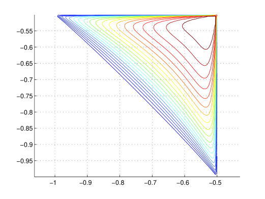
and compute numerically the third moment M3(γ1,γ2)subscript𝑀3subscript𝛾1subscript𝛾2M_{3}(\gamma_{1},\gamma_{2}) as given in Corollary 2.2. Figure 1 displays a contour plot of the third moment μ3(γ1,γ2)subscript𝜇3subscript𝛾1subscript𝛾2\mu_{3}(\gamma_{1},\gamma_{2}) in (5).

Refer to caption
Figure 1: Contour plot of μ3(γ1,γ2)subscript𝜇3subscript𝛾1subscript𝛾2\mu_{3}(\gamma_{1},\gamma_{2}).
Boundaries are given by the lines γ1=1/2subscript𝛾112\gamma_{1}=-1/2, γ2=1/2subscript𝛾212\gamma_{2}=-1/2 and γ1+γ2=3/2subscript𝛾1subscript𝛾232\gamma_{1}+\gamma_{2}=-3/2.

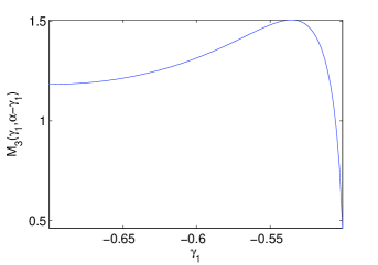
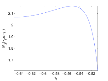
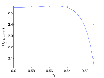
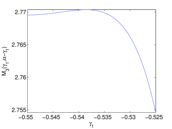
We shall also fix α=γ1+γ2𝛼subscript𝛾1subscript𝛾2\alpha=\gamma_{1}+\gamma_{2}, or equivalently, fix the Hurst index H=α+2𝐻𝛼2H=\alpha+2, and show that the third moment M3(γ1,γ2)subscript𝑀3subscript𝛾1subscript𝛾2M_{3}(\gamma_{1},\gamma_{2}) does change when γ1subscript𝛾1\gamma_{1} changes and γ2=αγ1subscript𝛾2𝛼subscript𝛾1\gamma_{2}=\alpha-\gamma_{1}.

In Tables 1-4 and Figures 1-4, we list and plot the values of

M3(γ1,αγ1)subscript𝑀3subscript𝛾1𝛼subscript𝛾1M_{3}(\gamma_{1},\alpha-\gamma_{1}) against γ1subscript𝛾1\gamma_{1} for H=0.6,0.7,0.8,0.9𝐻0.60.70.80.9H=0.6,0.7,0.8,0.9.
Remark 5.1.

Due to the symmetry, M3(γ1,γ2)=M3(γ2,γ1)subscript𝑀3subscript𝛾1subscript𝛾2subscript𝑀3subscript𝛾2subscript𝛾1M_{3}(\gamma_{1},\gamma_{2})=M_{3}(\gamma_{2},\gamma_{1}). Recall that γ1,γ2(1,1/2)subscript𝛾1subscript𝛾2112\gamma_{1},\gamma_{2}\in(-1,-1/2) with γ1+γ2>3/2subscript𝛾1subscript𝛾232\gamma_{1}+\gamma_{2}>-3/2. Thus α=γ1+γ2(3/2,1)𝛼subscript𝛾1subscript𝛾2321\alpha=\gamma_{1}+\gamma_{2}\in(-3/2,-1) and H=α+2(1/2,1)𝐻𝛼2121H=\alpha+2\in(1/2,1). In Tables 1-4 we let γ1subscript𝛾1\gamma_{1} take values from α/2𝛼2\alpha/2 to 0.5050.505-0.505.

Remark 5.2.

If γ1=γ2subscript𝛾1subscript𝛾2\gamma_{1}=\gamma_{2}, then γ1=γ2=α/2subscript𝛾1subscript𝛾2𝛼2\gamma_{1}=\gamma_{2}=\alpha/2, and M3(α/2,α/2)subscript𝑀3𝛼2𝛼2M_{3}(\alpha/2,\alpha/2) becomes the third moment of the standardized Rosenblatt distribution Zα/2(1)subscript𝑍𝛼21Z_{\alpha/2}(1) (see (1)). Its values (given in the first column in the tables) coincide with those obtained in Veillette and Taqqu (2013). See Table 4 of the supplement of Veillette and Taqqu (2013), where they are listed as a function of the parameter D=1H𝐷1𝐻D=1-H.

Since M3(γ1,γ2)subscript𝑀3subscript𝛾1subscript𝛾2M_{3}(\gamma_{1},\gamma_{2}) varies with γ1+γ2=αsubscript𝛾1subscript𝛾2𝛼\gamma_{1}+\gamma_{2}=\alpha fixed, we conclude that the class of generalized Hermite distributions is strictly richer than the class of Hermite distributions.

γ1subscript𝛾1\gamma_{1} -0.700 -0.678 -0.657 -0.635 -0.613 -0.592 -0.570 -0.548 -0.527 -0.505
M3(γ1,αγ1)subscript𝑀3subscript𝛾1𝛼subscript𝛾1M_{3}(\gamma_{1},\alpha-\gamma_{1}) 1.183 1.189 1.206 1.236 1.281 1.340 1.413 1.486 1.488 0.947
Table 1: M3(γ1,αγ1)subscript𝑀3subscript𝛾1𝛼subscript𝛾1M_{3}(\gamma_{1},\alpha-\gamma_{1}) when α=1.4𝛼1.4\alpha=-1.4 (or H=0.6𝐻0.6H=0.6).
Refer to caption
Figure 2: M3(γ1,αγ1)subscript𝑀3subscript𝛾1𝛼subscript𝛾1M_{3}(\gamma_{1},\alpha-\gamma_{1}) when α=1.4𝛼1.4\alpha=-1.4 (or H=0.6𝐻0.6H=0.6).
γ1subscript𝛾1\gamma_{1} -0.650 -0.634 -0.618 -0.602 -0.586 -0.569 -0.553 -0.537 -0.521 -0.505
M3(γ1,αγ1)subscript𝑀3subscript𝛾1𝛼subscript𝛾1M_{3}(\gamma_{1},\alpha-\gamma_{1}) 2.067 2.071 2.082 2.101 2.125 2.149 2.162 2.135 1.972 1.239
Table 2: M3(γ1,αγ1)subscript𝑀3subscript𝛾1𝛼subscript𝛾1M_{3}(\gamma_{1},\alpha-\gamma_{1}) when α=1.3𝛼1.3\alpha=-1.3 (or H=0.7𝐻0.7H=0.7).
Refer to caption
Figure 3: M3(γ1,αγ1)subscript𝑀3subscript𝛾1𝛼subscript𝛾1M_{3}(\gamma_{1},\alpha-\gamma_{1}) when α=1.3𝛼1.3\alpha=-1.3 (or H=0.7𝐻0.7H=0.7).
γ1subscript𝛾1\gamma_{1} -0.600 -0.589 -0.579 -0.568 -0.558 -0.547 -0.537 -0.526 -0.516 -0.505
M3(γ1,αγ1)subscript𝑀3subscript𝛾1𝛼subscript𝛾1M_{3}(\gamma_{1},\alpha-\gamma_{1}) 2.548 2.549 2.554 2.559 2.564 2.561 2.538 2.465 2.258 1.587
Table 3: M3(γ1,αγ1)subscript𝑀3subscript𝛾1𝛼subscript𝛾1M_{3}(\gamma_{1},\alpha-\gamma_{1}) when α=1.2𝛼1.2\alpha=-1.2 (or H=0.8𝐻0.8H=0.8).
Refer to caption
Figure 4: M3(γ1,αγ1)subscript𝑀3subscript𝛾1𝛼subscript𝛾1M_{3}(\gamma_{1},\alpha-\gamma_{1}) when α=1.2𝛼1.2\alpha=-1.2 (or H=0.8𝐻0.8H=0.8).
γ1subscript𝛾1\gamma_{1} -0.550 -0.545 -0.540 -0.535 -0.530 -0.525 -0.520 -0.515 -0.510 -0.505
M3(γ1,αγ1)subscript𝑀3subscript𝛾1𝛼subscript𝛾1M_{3}(\gamma_{1},\alpha-\gamma_{1}) 2.770 2.770 2.770 2.770 2.766 2.755 2.726 2.659 2.505 2.113
Table 4: M3(γ1,αγ1)subscript𝑀3subscript𝛾1𝛼subscript𝛾1M_{3}(\gamma_{1},\alpha-\gamma_{1}) when α=1.1𝛼1.1\alpha=-1.1 (or H=0.9𝐻0.9H=0.9).
Refer to caption
Figure 5: M3(γ1,αγ1)subscript𝑀3subscript𝛾1𝛼subscript𝛾1M_{3}(\gamma_{1},\alpha-\gamma_{1}) when α=1.1𝛼1.1\alpha=-1.1 (or H=0.9𝐻0.9H=0.9).

Acknowledgments. We would like to thank the referee for noting an error in the original version, and for some other comments leading to the improvement of the paper. This work was partially supported by the NSF grants DMS-1007616 and DMS-1309009 at Boston University.

References

  • Bai and Taqqu (2014a) S. Bai and M. Taqqu. The impact of diagonals of polynomial forms on limit theorems with long memory. arXiv preprint arXiv:1403.7544, 2014a.
  • Bai and Taqqu (2014b) S. Bai and M.S. Taqqu. Generalized Hermite processes, discrete chaos and limit theorems. Stochastic Processes and Their Applications, 124(4):1710–1739, 2014b.
  • Bai and Taqqu (2014c) S. Bai and M.S. Taqqu. Convergence of long-memory discrete k-th order Volterra processes. Preprint arXiv:1403.1903, 2014c.
  • Dobrushin and Major (1979) R.L. Dobrushin and P. Major. Non-central limit theorems for non-linear functional of Gaussian fields. Probability Theory and Related Fields, 50(1):27–52, 1979.
  • Ho and Hsing (1997) H. Ho and T. Hsing. Limit theorems for functionals of moving averages. The Annals of Probability, 25(4):1636–1669, 1997.
  • Maejima and Tudor (2012) M. Maejima and C.A. Tudor. Selfsimilar processes with stationary increments in the second Wiener chaos. Probability and Mathematical Statistics, 32(1):167–186, 2012.
  • Mori and Oodaira (1986) T. Mori and H. Oodaira. The law of the iterated logarithm for self-similar processes represented by multiple Wiener integrals. Probability theory and related fields, 71(3):367–391, 1986.
  • Nourdin and Peccati (2012) I. Nourdin and G. Peccati. Normal Approximations With Malliavin Calculus: From Stein’s Method to Universality. Cambridge Tracts in Mathematics. Cambridge University Press, 2012.
  • Rosenblatt (1961) M. Rosenblatt. Independence and dependence. In Proc. Fourth Berkeley Symp. Math. Statist. Probab, volume 2, pages 431–443, 1961.
  • Surgailis (1982) D. Surgailis. Zones of attraction of self-similar multiple integrals. Lithuanian Mathematical Journal, 22(3):327–340, 1982.
  • Taqqu (1975) M.S. Taqqu. Weak convergence to fractional Brownian motion and to the Rosenblatt process. Probability Theory and Related Fields, 31(4):287–302, 1975.
  • Taqqu (1979) M.S. Taqqu. Convergence of integrated processes of arbitrary Hermite rank. Probability Theory and Related Fields, 50(1):53–83, 1979.
  • Tudor (2013) C.A. Tudor. Analysis of Variations for Self-similar Processes: A Stochastic Calculus Approach. Springer, 2013.
  • Veillette and Taqqu (2013) M.S. Veillette and M.S. Taqqu. Properties and numerical evaluation of the Rosenblatt distribution. Bernoulli, 19(3):982–1005, 2013.

Shuyang Bai        bsy9142@bu.edu
Murad S. Taqqu   murad@bu.edu
Department of Mathematics and Statistics
111 Cumminton Street
Boston, MA, 02215, US