Perfect sampling algorithms for Schur processes

Abstract

We describe random generation algorithms for a large class of random combinatorial objects called Schur processes, which are sequences of random (integer) partitions subject to certain interlacing conditions. This class contains several fundamental combinatorial objects as special cases, such as plane partitions, tilings of Aztec diamonds, pyramid partitions and more generally steep domino tilings of the plane. Our algorithm, which is of polynomial complexity, is both exact (i.e. the output follows exactly the target probability law, which is either Boltzmann or uniform in our case), and entropy optimal (i.e. it reads a minimal number of random bits as an input).

The algorithm encompasses previous growth procedures for special Schur processes related to the primal and dual RSK algorithm, as well as the famous domino shuffling algorithm for domino tilings of the Aztec diamond. It can be easily adapted to deal with symmetric Schur processes and general Schur processes involving infinitely many parameters. It is more concrete and easier to implement than Borodin’s algorithm, and it is entropy optimal.

At a technical level, it relies on unified bijective proofs of the different types of Cauchy and Littlewood identities for Schur functions, and on an adaptation of Fomin’s growth diagram description of the RSK algorithm to that setting. Simulations performed with this algorithm suggest interesting limit shape phenomena for the corresponding tiling models, some of which are new.

1 Introduction

Tilings of the plane by pieces of prescribed shapes (such as dominos or rhombi) are fundamental combinatorial objects that have received much attention in discrete mathematics and computer science. In particular, several tiling problems have been studied as models of two dimensional statistical physics, mainly because their remarkable combinatorial structure makes these models physically interesting, algorithmically manageable, and mathematically tractable.

A celebrated example, introduced in [11], is given by domino tilings of the Aztec diamond, see Figure 1. The first remarkable property of this model is enumerative: the number of domino tilings of the Aztec diamond of size $n$ is $2^{\frac{n(n+1)}{2}}$. This property was proved in [11, 12] in several ways, but one of them is of particular importance for the present paper: this result can be proved using a bijective procedure, called the domino shuffling algorithm, that generates a tiling of the Aztec diamond of size $n$ taking exactly $\frac{n(n+1)}{2}$ bits as an input. This algorithm is not only elegant but also very useful, since it enabled the efficient sampling of large random tilings, and led to the empirical discovery of the arctic circle phenomenon later proved in [15].

Figure 1: Two domino tilings of the Aztec diamond of size $4$.

This paper deals with the extension of this picture to much more general models than that of the Aztec diamond. Indeed in recent years, many other models of tilings or related objects have been introduced and studied, mainly under the enumerative or “limit shape” viewpoint. In particular, it was recently observed that tilings of the Aztec diamond are part of a larger family of models of domino tilings of the plane, called steep tilings [7]. Steep tilings can themselves be represented as sequences of integer partitions known as Schur processes [23, 2], which puts them under the same roof as other well-known objects such as plane partitions [23, 24]. The latter have been much studied as well, and a very elegant and efficient strategy of enumeration and random generation for these objects follows from the Robinson–Schensted–Knuth (RSK) algorithm, see [28, Chap. 7]. Let us mention that the connection between tilings of the Aztec diamond and Schur processes is implicit in the work of Johansson [16]. We will also mention that both steep tilings and plane partitions can be seen as dimer matchings in the square and hexagonal lattices respectively. In recent work [6], it was observed that any Schur process (as defined below) can be realized as a dimer matching on a class of graphs called rail yard graphs.

Our main result, algorithm SchurSample of Section 3, is a random generation algorithm for general Schur processes. Remarkably, the algorithm is a common generalization of both the RSK-based strategy for plane partitions and of the domino shuffling algorithm, thus putting those two well-studied combinatorial algorithms under the same roof. It enables one to efficiently sample large random configurations, which at the empirical level unveils some new properties of their limit shapes. Theorem 3.2 proves correctness.

At a technical level, our main tools are combinatorial constructions dealing with integer partitions subject to interlacing conditions, that can be viewed as bijective proofs of the different Cauchy identities for Schur functions. The obtained algorithm takes as an input a finite sequence of geometric random variables and random bits that can be represented in a graphical way in terms of growth diagrams similar to Fomin’s description of the RSK algorithm, see e.g. [28, Appendix]. In this setting, it is easy to see that the algorithm is entropy optimal (Proposition 3.8). The (polynomial) complexity is also studied (Proposition 3.6).

We then adapt our algorithm in order to produce samples from symmetric Schur processes. These processes are defined on symmetric sequences of partitions, or in a different interpretation on free boundary sequences. They are related to free boundary or symmetric tilings of the plane. Examples include symmetric plane partitions and plane overpartitions. We produce the SymmetricSchurSample algorithm and two variants in Section 4. The modifications we make to obtain these algorithms are related to the Littlewood identities for Schur functions and allow us to obtain generalizations of the symmetric RSK algorithm. Other adaptations of our algorithm are discussed in Sections 5 and 6, and correspond to limiting cases such as unboxed plane partitions or Plancherel-type measures.

We conclude this introduction with references to previous works, and a discussion on how this paper relates to them. The idea of growing Schur processes dynamically has been floating around even before these objects were invented, in the context of the RSK correspondence, and was the subject of several papers. Gessel [13], Krattenthaler [18], Pak–Postnikov [25], and Fomin [28, Chap.7] all discuss RSK-type bijections that are based on a growing procedure, and could be used for sampling special kinds of Schur processes corresponding to the primal-RSK and dual-RSK situation (and indeed in the primal-case of Section 3, the basic building-block we are using is Gessel’s bijection). However, those works do not contain a growing procedure for these objects that both covers the mixed primal/dual case and that is totally concrete and bijective. The first motivation of this paper is to fill this gap, and this level of concreteness enables us to transform the growing procedure into an effective sampling algorithm, that we have entirely implemented.

In a different context, Borodin [2] gives a random sampling algorithm for fully general Schur processes. It is also based on a growing procedure and similarly uses geometric random variables as an input, but contrarily to ours it is not entropy optimal (although this question is not discussed in [2], it is easy to see by comparing with the present paper). Our algorithm, which is based only on two very explicit simple growing rules, is arguably easier to implement. Its simplicity and its entropic efficiency are the second motivation for our work. Let us also note that growing dynamics have been described for generalizations of Schur processes such as Macdonald processes, see e.g. the recent paper of Borodin and Petrov [5], at the cost of an increase in complexity and entropy (and atomic steps are no longer bijections). Finally, RSK-type dynamics have also been a useful tool in the analysis of various probabilistic models [14, 21].

A last situation (maybe more surprisingly related to ours) where growing procedures were employed arises in the study of the Aztec diamond. As mentioned above, Elkies–Kuperberg–Larsen–Propp’s domino shuffling algorithm [12] is a procedure that enables one to recursively grow uniform tilings of an Aztec diamond of increasing size. Initially invented as a combinatorial device with miraculous properties, the Aztec diamond is now understood to be part of a large class of domino tilings of the plane [7] in bijection with certain Schur processes. As it turns out, the domino shuffling algorithm can be viewed as a special case of our growth procedure, thus revealing a part of the structure hidden behind this algorithm (another part is given by the connection with cluster algebras [27]). The third motivation of this paper is therefore to put the domino shuffling under the same roof as growing procedures for Schur processes and the RSK correspondences.

To be complete, let us finally mention a few previous works related to the sampling of tilings of the plane that are not directly related to ours. Propp and Wilson’s coupling from the past method [26] is often used for random sampling of domino tilings. In a different direction, the reader interested in exhaustive sampling of tilings (outside the realm of Schur processes) could consult [10] and references therein.

The paper is organized as follows. In Section 2 we remind the definition of Schur processes and explain its relation to tilings through examples. We also describe the necessary prerequisites on partitions, Schur functions and the vertex operator formalism needed in the rest of the paper. In Section 3 we give the main sampling algorithm for Schur processes after initially describing the two main bijections we use in said algorithm. We also give some samples of large tilings obtained using these algorithms. In Section 4 we modify the algorithm to suit symmetric (free boundary) Schur processes and provide some samples obtained using the algorithms. We discuss sampling from the so-called unbounded Schur process in Section 5 and from the most general Schur process in Section 6. We conclude in Section 7.

2 Reminders on Schur processes

2.1 Basic definitions

A partition $\lambda$ is a nonincreasing sequence of nonnegative integers $\lambda_{1}\geq\lambda_{2}\geq\cdots$ that vanishes eventually. We call each positive $\lambda_{i}$ a part and the number of parts, called the length of $\lambda$, is denoted $\ell(\lambda)$. The empty partition $\emptyset$ is the partition of length zero. We call $|\lambda|:=\sum_{i=1}^{\ell(\lambda)}\lambda_{i}$ the weight of the partition. For any $\lambda$ we have a conjugate partition $\lambda^{\prime}$ whose parts are defined as $\lambda^{\prime}_{i}:=|\{j:\lambda_{j}\geq i\}|$. It is often convenient to represent partitions graphically by either Young or Maya diagrams, see Figure 2. A Maya diagram is an encoding of a partition $\lambda$ as a boolean function $\mathbb{Z}+\frac{1}{2}\to\{\circ,\bullet\}$, where particles $\bullet$ are assigned to the half-integers of the form $\lambda_{i}-i+1/2+n$, $i=1,2,\dots$ and holes $\circ$ to all the others, for some integer $n$. Starting with a Maya diagram one recovers parts of the partition by counting the number of holes to the left of each particle. The positions of the holes actually encode the conjugate partition, being precisely the half-integers of the form $-\lambda^{\prime}_{i}+i+1/2+n$, $i=1,2,\dots$.

(a)

(b)

(c)

Figure 2: The Young diagram of the partition $(2,2,2,1,1)$ shown in: (a) English convention, (b) French convention and (c) Russian convention and a Maya diagram associated to it.

Let $\lambda$ and $\mu$ be two partitions with $\lambda\supseteq\mu$ (that is, $\lambda_{i}\geq\mu_{i}$ for all $i$). They are said to be interlacing and we write $\lambda\succ\mu$ if and only if $\lambda_{1}\geq\mu_{1}\geq\lambda_{2}\geq\mu_{2}\geq\lambda_{3}\geq\cdots$. The interlacing property is equivalent to saying that the skew diagram $\lambda/\mu$ (the set-difference of the Young diagrams of $\lambda$ and $\mu$) is a horizontal strip, i.e. it has at most one square in each column. There is a notion of dual interlacing: we write $\lambda\succ^{\prime}\mu$ if $\lambda^{\prime}\succ\mu^{\prime}$, or equivalently if the skew diagram $\lambda/\mu$ is a vertical strip, i.e.  $0\leq\lambda_{i}-\mu_{i}\leq 1$ for all $i$.

For a word $w=(w_{1},w_{2},\dots,w_{n})\in\{\prec,\succ,\prec^{\prime},\succ^{\prime}\}^{n}$, we say that a sequence of partitions $\Lambda=(\emptyset=\lambda(0),\lambda(1),\dots,\lambda(n)=\emptyset)$ is $w$-interlaced if $\lambda(i-1)\,w_{i}\,\lambda(i)$, for $i=1,\dots,n$. Also, word multiplication is defined as concatenation, e.g. $(\prec)^{3}(\prec^{\prime},\succ)^{2}=(\prec,\prec,\prec,\prec^{\prime},\succ,\prec^{\prime},\succ)$. We are now ready to define Schur processes.

Definition 2.1.

For a word $w=(w_{1},w_{2},\dots,w_{n})\in\{\prec,\succ,\prec^{\prime},\succ^{\prime}\}^{n}$, the Schur process of word $w$ with parameters $Z=(z_{1},\dots,z_{n})$ is the measure on the set of $w$-interlaced sequences of partitions $\Lambda=(\emptyset=\lambda(0),\lambda(1),\dots,\lambda(n)=\emptyset)$ given by

$$Prob(\Lambda)\propto\prod_{i=1}^{n}z_{i}^{||\lambda(i)|-|\lambda(i-1)||}.$$ (2.1)

Remark 2.2.

There is actually a more general definition of Schur processes [23, 2] which we discuss in Section 5. The definition we use for the moment covers most applications, and is actually the same one for which other exact sampling algorithms were given in [2, Section 7].

The most natural specialization of the measure (2.1) (which also ensures convergence) is obtained by choosing a parameter $0<q<1$ and then choosing the $z_{i}$ parameters such that

$$Prob(\Lambda)\propto q^{\text{Volume}(\Lambda)}=q^{\sum_{i}|\lambda(i)|}.$$

This can be accomplished by choosing

$$z_{i}=\left\{\begin{array}[]{ll}q^{-i}&\text{if }w_{i}\in\{\prec,\prec^{\prime}\}\\ q^{i}&\text{if }w_{i}\in\{\succ,\succ^{\prime}\}\\ \end{array}.\right.$$ (2.2)

For some concrete words there might be other, more convenient, choices of $z_{i}$ that also give the $q^{\text{Volume}}$ weight.

Before we proceed with examples, we introduce an encoded shape associated with $w=(w_{1},w_{2},\dots,w_{n})\in\{\prec,\succ,\prec^{\prime},\succ^{\prime}\}^{n}$. Construct a path consisting of horizontal and vertical unit length segments, choosing a horizontal segment if $w_{i}\in\{\prec,\prec^{\prime}\},$ and vertical if $w_{i}\in\{\succ,\succ^{\prime}\}$, and moving in the right-downward direction, as in Figure 3. This path can be seen as the boundary of a Young diagram (in French convention) which we call the encoded shape and denote with $sh(w)$. It is not hard to see that parts of the partition corresponding to $sh(w)$ are obtained by counting the number of $\{\prec,\prec^{\prime}\},$ elements of $w$ lying to the left of a fixed $w_{i}\in\{\succ,\succ^{\prime}\}$.

Figure 3: The encoded shape of $w=(\prec,\prec^{\prime},\succ,\succ^{\prime},\prec,\succ^{\prime},\prec,\succ^{\prime})$ is $sh(w)=(4,3,2,2)$.

2.2 Examples

There are several special cases of interest, listed below. They all correspond to various types of tilings.

Reverse plane partitions

of shape $\mathcal{S}$, where $\mathcal{S}$ is a Young diagram in French convention, are fillings of $\mathcal{S}$ with nonnegative integers that form nondecreasing rows and columns, see Figure 4. In other words, if squares in $\mathcal{S}$ are represented with their position $(i,j)$ ($i$ being the row and $j$ the column the square belongs to, where the bottom-left square is represented with (1,1)), and $\pi_{i,j}$ is the filling of $(i,j)$, then we have $\pi_{i,j}\leq\pi_{k,l}$ whenever $i\leq k$ and $j\leq l$.

For $w\in\{\prec,\succ\}^{n}$, it is not hard to see that $w$-interlaced sequences are in correspondence with reverse plane partitions of shape $sh(w)$, also know as skew plane partitions when zero fillings are ignored. The corresponding interlacing partitions are diagonal slices of the reverse plane partition.

In particular, reverse plane partitions of shape $m^{n}=(\overbrace{m,\dots,m}^{n})$, which are also known as $(m\times n)$-boxed plane partitions, correspond to $w$-interlaced sequence where $w=(\prec)^{m}(\succ)^{n}$.

Figure 4: A reverse plane partition of shape (5,5,3,3) corresponding to the interlacing sequence $\emptyset\prec(1)\prec(3,1)\prec(4,2)\succ(2,2)\succ(2)\prec(3,2)\prec(4,2)\succ(2)\succ\emptyset$.

Domino tilings of the Aztec diamond

of size $n$ are in correspondence with $w$-interlaced sequences where $w=(\prec^{\prime},\succ)^{n}$. The correspondence is described in the part about steep tilings, see Figure 7(a) for illustration of the correspondence. The encoded shape is a staircase partition, i.e. $(n,n-1,\dots,1)$. Notice that since the number of tilings is bounded, there are no convergence issues and one can get any general Schur distribution with generic $Z$ parameters.

Pyramid partitions

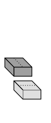
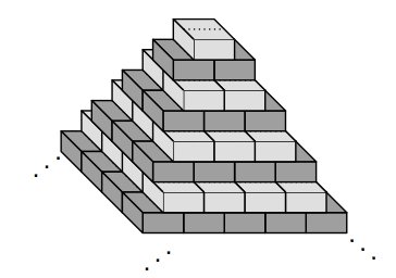
[30] are infinite heaps of blocks of size $2\times 2\times 1$ stacked in a way that resembles pyramids. For a precise definition we first start with a minimal pyramid partition that is an infinite heap of blocks shown in Figure 5(b). For convenience, we use two different colors to represent odd layers versus even layers. A pyramid partition is obtained by removing a finite number of blocks from the minimal pyramid partition where a block can be removed if there are no blocks on top of it, see Figure 5(c) for an example.

(a)

(b)

(c)

Figure 5: Building blocks (a), a minimal pyramid partition (b), a pyramid partition (c).

A view from the top of a pyramid partition reveals a domino tiling corresponding to the pyramid partition, see Figure 6.

Figure 6: Domino tilings corresponding to the pyramid partitions from Figure 5.

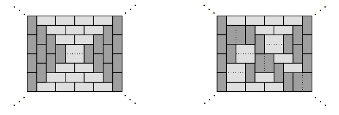
A pyramid partition of width $l$ is obtained from the minimal pyramid partition by removing blocks that lie inside the strip $-l\leq x-y\leq l$, where the center of the top block is placed at (0,0), see Figure 6.

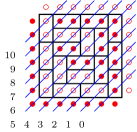
It can be shown that pyramid partitions of width $l$ correspond to $w$-interlaced sequences where $w=(\underbrace{\dots,\prec,\prec^{\prime},\prec,\prec^{\prime}}_{l},\underbrace{\succ,\succ^{\prime},\succ,\succ^{\prime},\dots}_{l})$. See Figure 7(b) for an illustration of the correspondence which is explained below, in the part about steep tilings.

(a)

(b)

Figure 7: (a) A $2\times 2$ Aztec diamond corresponding to the sequence $\emptyset\prec^{\prime}(1,1)\succ(1)\prec^{\prime}(2)\succ\emptyset$. (b) A pyramid partition of width 5 corresponding to the sequence $\emptyset\prec^{\prime}(1)\prec(1,1)\prec^{\prime}(2,2)\prec(2,2,2)\prec^{\prime}(3,3,2)\succ(3,2)\succ^{\prime}(2,1)\succ(2)\succ^{\prime}(1)\succ\emptyset$.

Steep tilings

generalize both Aztec diamonds and pyramid partitions, and are roughly speaking domino tilings of a strip. Before we proceed with a precise definition we introduce some conventions. Assume we are given a domino tiling of a square grid and that the grid is colored in a chessboard fashion. A domino is called positive if its top-left corner belongs to a white square, otherwise the domino is called negative. Also, if a square belongs to a positive domino then to its center we assign a hole $\circ$, otherwise we assign a particle $\bullet$.

Let a word $w=(w_{1},\dots,w_{2l})\in\{\prec,\succ,\prec^{\prime},\succ^{\prime}\}^{2l}$ be such that $w_{2i}\in\{\prec,\succ\}$ and $w_{2i+1}\in\{\prec^{\prime},\succ^{\prime}\}$. Construct a path of length $2l$ consisting of horizontal and vertical unit length segments for each $i=1,\dots,2l$ by choosing a horizontal segment if

$$w_{i}=\left\{\begin{array}[]{ll}\prec^{\prime}&\text{if }i\text{ is odd},\\ \succ&\text{if }i\text{ is even}\\ \end{array}\right.$$

and vertical otherwise, and moving in the right-downward direction, as in Figure 8. Then add an infinite strip of dominoes like in Figure 8. We call this domino tiling a $w$-minimal tiling. Up and to the right of the path are positive dominoes and down and to the left are negative dominoes.

Figure 8: A $w$-minimal tiling for $w=(\prec^{\prime},\prec,\prec^{\prime},\prec,\prec^{\prime},\succ,\succ^{\prime},\succ,\prec^{\prime},\prec)$.

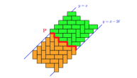
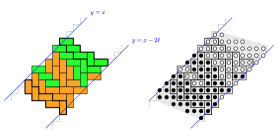
A $w$-steep tiling is a domino tiling obtained from the $w$-minimal tiling by performing finitely many flips, i.e. by replacing a pair of two adjacent vertical dominoes with a pair of two adjacent horizontal dominoes or vice versa. One such example is shown in Figure 9. If we assign particles and holes as described above, we get a representation of a steep tiling as a sequence of partitions (where each diagonal slice is a partition represented by its Maya diagram), see Figure 9.

Figure 9: A $w$-steep tiling for $w=(\prec^{\prime},\prec,\prec^{\prime},\prec,\prec^{\prime},\succ,\succ^{\prime},\succ,\prec^{\prime},\prec).$

.

Let $w=(w_{1},\dots,w_{2l})$ be such that $w_{2i}\in\{\prec,\succ\}$ and $w_{2i+1}\in\{\prec^{\prime},\succ^{\prime}\}$. Using the correspondence shown in Figure 9, it can be shown that $w$-step tilings are in bijection with $w$-interlaced sequences, see [7] for details of the proof. In particular, $w=(\prec^{\prime},\succ)^{n}$ corresponds to $n\times n$ Aztec diamonds and $w=(\prec^{\prime},\prec)^{l}(\succ^{\prime},\succ)^{l}$ to pyramid partitions of width $2l$.

2.3 Schur processes via symmetric functions and vertex operators

Schur processes can be defined using tools coming from representation theory or theoretical physics, namely Schur symmetric functions and vertex operators. We present this here.

We start with the definition of Schur functions, which can be defined in many ways, for example using the Jacobi–Trudi formula, see e.g. [19],

$$s_{\lambda}(x_{1},\dots,x_{n})=\det_{1\leq i,j\leq n}h_{\lambda_{i}-i+j}(x_{1},\dots,x_{n}).$$ (2.3)

Here the $h$’s are the complete symmetric functions. By convention $s_{\emptyset}(\cdot)=1$ and $s_{\lambda}()=\delta_{\lambda,\emptyset}$. We only give the definition for finitely many variables as this is enough for our purposes. Related are the skew Schur functions, which for two partitions $\lambda,\mu$ are zero unless $\mu\subseteq\lambda$, in which case they are defined by

$$s_{\lambda/\mu}(x_{1},\dots,x_{n})=\det_{1\leq i,j\leq n}h_{\lambda_{i}-\mu_{j}-i+j}(x_{1},\dots,x_{n}).$$ (2.4)

Note that $s_{\lambda/\emptyset}=s_{\lambda}$. Let us denote the alphabet $(x_{1},\dots,x_{n})$ by $X$ (and similarly for $Y$). For our purposes, the important identities satisfied by Schur functions are the branching rule

$$s_{\lambda/\mu}(X,Y)=\sum_{\nu}s_{\lambda/\nu}(X)s_{\nu/\mu}(Y)$$ (2.5)

and the Cauchy (and dual Cauchy) identities:

$$\sum_{\nu}s_{\nu/\lambda}(X)s_{\nu/\mu}(Y) =\prod_{i,j}\frac{1}{1-x_{i}y_{j}}\sum_{\kappa}s_{\lambda/\kappa}(Y)s_{\mu/\kappa}(X),$$ (2.6)

$$\sum_{\nu}s_{\nu/\lambda}(X)s_{\nu^{\prime}/\mu^{\prime}}(Y) =\prod_{i,j}(1+x_{i}y_{j})\sum_{\kappa}s_{\lambda^{\prime}/\kappa^{\prime}}(Y)s_{\mu/\kappa}(X).$$ (2.7)

Schur functions can also be defined as a generating series of semi-standard Young tableaux. Precisely, for $\mu\subseteq\lambda$,

$$s_{\lambda/\mu}(x_{1},\dots,x_{n})=\sum_{T}x_{i}^{\#\ \text{of}\ i\ \text{in}\ T},$$ (2.8)

where the sum ranges over all semi-standard Young tableaux of shape $\lambda/\mu$ (fillings of the skew diagram $\lambda/\mu$ with numbers 1 through $n$ such that the numbers weakly increase in rows, from left to right, and strictly increase down columns). Note that, in one variable, we have

$$s_{\lambda/\mu}(x_{1})=x_{1}^{|\lambda|-|\mu|}\delta_{\lambda\succ\mu}.$$ (2.9)

The fact that the two definitions are equivalent is the content of the Lindström–Gessel–Viennot lemma, see e.g. [28]. The Cauchy identities can be proven from the tableaux definition using the RSK correspondence [17].

In the infinite wedge formalism (we refer the reader to, e.g., [23, 24] for details), to each partition $\lambda$ one associates a basis vector $|\lambda\rangle$ (respectively covector $\langle\lambda|$) in the half-infinite wedge vector space denoted in the literature by $\bigwedge^{\frac{\infty}{2}}V$ (respectively in the dual vector space). We add a bilinear form defined by $\langle\lambda|\mu\rangle=\delta_{\lambda,\mu}$. Two important operators, each depending on a parameter, acting on these vectors are $\Gamma_{+}(z)$ and $\Gamma_{-}(z)$. We call them vertex operators. Operator $\Gamma_{+}(z)$ removes, in all possible ways, a horizontal strip with weight $z^{\#\ \text{boxes}}$ from a partition. Operator $\Gamma_{-}(z)$ adds a horizontal strip. More precisely, we have

$$\Gamma_{+}(z)|\lambda\rangle:=\sum_{\mu\prec\lambda}z^{|\lambda|-|\mu|}|\mu\rangle,\qquad\Gamma_{-}(z)|\lambda\rangle:=\sum_{\mu\succ\lambda}z^{|\mu|-|\lambda|}|\mu\rangle.$$

We also define operators $\tilde{\Gamma}_{+}(z)$ and $\tilde{\Gamma}_{-}(z)$ which respectively remove or add vertical strips, i.e.

$$\tilde{\Gamma}_{+}(z)|\lambda\rangle:=\sum_{\mu\prec^{\prime}\lambda}z^{|\lambda|-|\mu|}|\mu\rangle,\qquad\tilde{\Gamma}_{-}(z)|\lambda\rangle:=\sum_{\mu\succ^{\prime}\lambda}z^{|\mu|-|\lambda|}|\mu\rangle.$$

Using the tableaux definition, or the branching rule, one can show that Schur functions take the following form in terms of the $\Gamma$ operators:

$$s_{\lambda/\mu}(x_{1},\dots,x_{n}) =\langle\mu|\Gamma_{+}(x_{1})\cdots\Gamma_{+}(x_{n})|\lambda\rangle=\langle\lambda|\Gamma_{-}(x_{1})\cdots\Gamma_{-}(x_{n})|\mu\rangle,$$ (2.10)

$$s_{\lambda^{\prime}/\mu^{\prime}}(x_{1},\dots,x_{n}) =\langle\mu|\tilde{\Gamma}_{+}(x_{1})\cdots\tilde{\Gamma}_{+}(x_{n})|\lambda\rangle=\langle\lambda|\tilde{\Gamma}_{-}(x_{1})\cdots\tilde{\Gamma}_{-}(x_{n})|\mu\rangle.$$ (2.11)

Observe the action of these operators on the vacuum vector (empty partition vector):

$$\Gamma_{+}(x)|\emptyset\rangle=\tilde{\Gamma}_{+}(x)|\emptyset\rangle=|\emptyset\rangle,\ \langle\emptyset|\Gamma_{-}(y)=\langle\emptyset|\tilde{\Gamma}_{-}(y)=\langle\emptyset|.$$ (2.12)

The following commutation relations hold:

$$\Gamma_{+}(x)\Gamma_{-}(y) =\frac{1}{1-xy}\Gamma_{-}(y)\Gamma_{+}(x),$$ (2.13)

$$\tilde{\Gamma}_{+}(x)\tilde{\Gamma}_{-}(y) =\frac{1}{1-xy}\tilde{\Gamma}_{-}(y)\tilde{\Gamma}_{+}(x),$$ (2.14)

$$\tilde{\Gamma}_{+}(x)\Gamma_{-}(y) =(1+xy)\Gamma_{-}(y)\tilde{\Gamma}_{+}(x),$$ (2.15)

$$\Gamma_{+}(x)\tilde{\Gamma}_{-}(y) =(1+xy)\tilde{\Gamma}_{-}(y)\Gamma_{+}(x).$$ (2.16)

They also satisfy the trivial commutation relations whereby any two operators whose indices are the same (both $+$ or both $-$) commute, regardless of parameters.

It is not hard to see that the commutation relations (2.13) and (2.15) are equivalent to the Cauchy (2.6) and dual Cauchy (2.7) identities. Obviously this is true when $X=(x)$ and $Y=(y)$, and in general this is true by the branching rule, eqs. 2.10 and 2.11. The other two commutation relations are also equivalent to the Cauchy identities by just conjugating all the partitions involved. In Section 3 we will describe bijections that allow us to give (bijective) proofs of the commutation relations, which we further use to obtain our exact sampling algorithm.

The Schur process of word $w$ with parameters $Z$ can be written as

$$Prob(\Lambda)\propto\prod_{i=1}^{n}\langle\lambda(i-1)|\Gamma_{i}(z_{i})|\lambda(i)\rangle$$ (2.17)

where $\Gamma_{i}$ is $\Gamma_{+}$, $\Gamma_{-}$, $\tilde{\Gamma}_{+}$, $\tilde{\Gamma}_{-}$ if $w_{i}$ is $\prec,\succ,\prec^{\prime},\succ^{\prime}$, respectively. The partition function is given by

$$Z_{w}=\sum_{\Lambda}\prod_{i=1}^{n}z_{i}^{||\lambda(i)|-|\lambda(i-1)||}=\langle\emptyset|\prod_{i=1}^{n}\Gamma_{i}(z_{i})|\emptyset\rangle.$$ (2.18)

A simple application of the above commutation relations, along with the action of the vertex operators on the vacuum vectors (2.12) yields:

Proposition 2.3.

The partition function of the Schur process of word $w$ with parameters $Z$ is equal to

$$Z_{w}=\prod_{i<j,w_{i}\in\{\prec,\prec^{\prime}\},w_{j}\in\{\succ,\succ^{\prime}\}}(1+\epsilon_{i,j}z_{i}z_{j})^{\epsilon_{i,j}},$$ (2.19)

where $\epsilon_{i,j}=1$ if $(w_{i},w_{j})\in\{(\prec,\succ^{\prime}),(\prec^{\prime},\succ)\}$ and $\epsilon_{i,j}=-1$ otherwise.

3 Bijective sampling of Schur processes

Exact sampling algorithms based on partition processes for classes of tilings including plane and skew plane partitions [2] (see also [4] for a general approach and [3] for an application of this approach to a restricted class of graphs including, but not limited to, the Aztec diamond graph) and Aztec diamonds (see [12] and remark below) have been proposed before. There is also the coupling from the past approach of Propp and Wilson [26]. In this section we give an overall encompassing algorithm for Schur processes (different from, but similar to, that of [2]) which under appropriate specializations gives exact random sampling of plane (and skew plane) partitions, Aztec diamonds, pyramid partitions and more generally, steep tilings.

Our algorithm is based on bijective proofs of the Cauchy identities for Schur functions, which, as we have explained earlier, are equivalent to the commutation relations between $\Gamma_{+}(x)$ and $\Gamma_{-}(y)$, or, in the dual case, between $\Gamma_{+}(x)$ and $\tilde{\Gamma}_{-}(y)$. Bijections are represented schematically in Figure 10, and the corresponding commutation relations on which they are based in Figure 11. They are given in simple terms and lead to an algorithm that is easy to implement. We note that bijective proofs of Cauchy identities and versions of bijections we describe here appeared earlier in the literature. For the work related to the Cauchy case see Gessel [13], and work related to the dual case see Pak–Postnikov [25] and Krattenthaler [18]. Recent work of Borodin–Petrov [5] puts the Cauchy case in the more general framework of nearest neighbor dynamics. In particular, in Section 7 they provide two bijections for the Cauchy case (one listed below), both of which could be used for a sampling algorithm.

(a)

(b)

Figure 10: A diagrammatic representation of the two bijections. In the Cauchy case (a) we map a pair $(\kappa,G)$ such that $\lambda\succ\kappa\prec\mu$ and $G\in\mathbb{N}$ to $\nu$ such that $\lambda\prec\nu\succ\mu$. In the dual Cauchy case (b) we map a pair $(\kappa,B)$ such that $\lambda\succ^{\prime}\kappa\prec\mu$ and $B\in\{0,1\}$ to $\nu$ such that $\lambda\prec\nu\succ^{\prime}\mu$.

(a)

(b)

Figure 11: The atomic commutation relations of $\Gamma_{+}(x)$ and $\Gamma_{-}(y)$ (a), and of $\Gamma_{+}(x)$ and $\tilde{\Gamma}_{-}(y)$ (b); $G\in\mathbb{N},B\in\{0,1\}$.

Cauchy case

Let $\lambda,\kappa,\mu$ be three partitions such that $\lambda\succ\kappa,\mu\succ\kappa$ and let $G\in\mathbb{N}$. We describe a procedure for building a fourth partition $\nu$ with the properties that $\lambda\prec\nu,\mu\prec\nu$ and $|\lambda|+|\mu|+G=|\kappa|+|\nu|$, in such a way that the mapping $(\kappa,G)\mapsto\nu$ is bijective (i.e. every possible $\nu$ is obtained once and exactly once by the procedure). See Figure 10-a for a schematic representation. We construct $\nu$ (which has at most $\max(\ell(\lambda),\ell(\mu))+1$ parts) by setting

$$\nu_{i}=\begin{cases}\max(\lambda_{1},\mu_{1})+G&\text{if $i=1$},\\ \max(\lambda_{i},\mu_{i})+\min(\lambda_{i-1},\mu_{i-1})-\kappa_{i-1}&\text{if $i>1$}\\ \end{cases}$$ (3.1)

and it is readily checked that the wanted properties hold.

Using the bijection we deduce

$$\sum_{\begin{subarray}{c}\nu\\ \nu\succ\lambda\\ \nu\succ\mu\end{subarray}}x^{|\nu|-|\lambda|}y^{|\nu|-|\mu|}=\sum_{G\geq 0}\sum_{\begin{subarray}{c}\kappa\\ \kappa\prec\lambda\\ \kappa\prec\mu\end{subarray}}x^{|\mu|-|\kappa|+G}y^{|\lambda|-|\kappa|+G}=\frac{1}{1-xy}\sum_{\begin{subarray}{c}\kappa\\ \kappa\prec\lambda\\ \kappa\prec\mu\end{subarray}}x^{|\mu|-|\kappa|}y^{|\lambda|-|\kappa|}.$$ (3.2)

This identity amounts to the commutation relation (2.13), and to the Cauchy identity (2.6) in the case where $X$ and $Y$ are reduced to a single variable.

To obtain a bijective proof of the commutation relation (2.14), one applies the same procedure after a priori conjugating all the partitions and conjugating the resulting $\nu$ at the end.

The first bijective procedure (proving (2.13)) has time complexity $O(\ell(\nu))$ while the second (proving (2.14)) is $O(\max(\ell(\nu),\nu_{1}))$ so both are commonly $O(\max(\ell(\nu),\nu_{1}))$ (and we will need this weaker bound in order to give uniform estimates below).

The above bijection can be turned into a random sampling procedure easily. With the notation set up above, define a method sampleHH (HH stands for horizontal-horizontal and the fact that we are commuting $\Gamma_{+}$ and $\Gamma_{-}$) that does the following:

def sampleHH($\lambda,\mu,\kappa,\xi$)
sample $G\sim Geom(\xi)$
construct $\nu$ based on the bijective procedure described above
return $\nu$

where $Geom(\xi)$ samples a single geometric random variable from the distribution $Prob(k)\propto\xi^{k}$ (we assume $0\leq\xi<1$). Then applying this procedure for $\xi=xy$ will produce $\nu$ distributed as $Prob(\nu)\propto s_{\nu/\lambda}(x)s_{\nu/\mu}(y)$ using minimal entropy (the sampling of a single geometric random variable) and assuming $\lambda,\nu,\kappa$ are coming from a Schur process, in the end so will $\nu$ (from a different Schur process, of course).

A method sampleVV can be defined in the same way and corresponds to commuting $\tilde{\Gamma}_{+}$ and $\tilde{\Gamma}_{-}$.

Dual Cauchy case

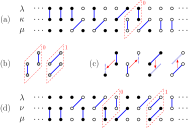
Let $\lambda,\kappa,\mu$ be three partitions such that $\kappa\prec^{\prime}\lambda,\mu\succ\kappa$ and let $B\in\{0,1\}$. We describe a procedure similar to the above one for building a fourth partition $\nu$ with the properties that $\lambda\prec\nu,\mu\prec^{\prime}\nu$ and $|\lambda|+|\mu|+B=|\kappa|+|\nu|$, in such a way that the mapping $(\kappa,B)\mapsto\nu$ is bijective. See Figure 10-b for a schematic representation. Here we directly define the method sampleHV (HV stands for horizontal-vertical and the fact that we are commuting $\Gamma_{+}$ and $\tilde{\Gamma}_{-}$):

def sampleHV($\lambda,\mu,\kappa,\xi$)
sample $B\sim Bernoulli(\frac{\xi}{1+\xi})$
for $i=1\dots\max(\ell(\lambda),\ell(\mu))+1$
if $\lambda_{i}\leq\mu_{i}<\lambda_{i-1}$ then $\nu_{i}=\max(\lambda_{i},\mu_{i})+B$
else $\nu_{i}=\max(\lambda_{i},\mu_{i})$
if $\mu_{i+1}<\lambda_{i}\leq\mu_{i}$ then $B=\min(\lambda_{i},\mu_{i})-\kappa_{i}$
return $\nu$

where $Bernoulli(\xi)$ is a Bernoulli random variable that returns 0 with probability $1-\xi$ and 1 with probability $\xi$. To check the validity of our method, note first that the interlacing conditions for $\kappa$ and $\nu$ amount to

$$\max(\lambda_{i}-1,\mu_{i+1})\leq\kappa_{i}\leq\min(\lambda_{i},\mu_{i}),\quad\max(\lambda_{i},\mu_{i})\leq\nu_{i}\leq\min(\lambda_{i-1},\mu_{i}+1)$$

where by convention $\lambda_{0}=\infty$. In particular, the quantity $\min(\lambda_{i},\mu_{i})-\kappa_{i}$ vanishes unless

$$\mu_{i+1}<\lambda_{i}\leq\mu_{i}$$ (3.3)

in which case it may also take the value $1$. Let $i_{1}<i_{2}<\cdots<i_{r}$ be the $i$’s such that (3.3) holds. Similarly, the quantity $\nu_{i}-\max(\lambda_{i},\mu_{i})$ vanishes unless

$$\lambda_{i}\leq\mu_{i}<\lambda_{i-1}$$ (3.4)

in which case it may also take the value $1$. Let $j_{1}<j_{2}<\cdots<j_{s}$ be the $i$’s such that (3.4) holds. Our method works provided that $s=r+1$ and

$$j_{1}\leq i_{1}<j_{2}\leq i_{2}<\cdots<j_{r}\leq i_{r}<j_{r+1},$$ (3.5)

which follows from the easily checked fact that the mapping

$$i\mapsto\min\{j>i,\lambda_{j}\leq\mu_{j}\}$$

defines a bijection between $\{0,i_{1},i_{2},\ldots,i_{r}\}$ and $\{j_{1},j_{2},\ldots,j_{s}\}$. The $(\kappa,B)\mapsto\nu$ bijection implies

$$\sum_{\begin{subarray}{c}\nu\\ \nu\succ\lambda\\ \mu\prec^{\prime}\nu\end{subarray}}x^{|\nu|-|\lambda|}y^{|\nu|-|\mu|}=\sum_{B\in\{0,1\}}\sum_{\begin{subarray}{c}\kappa\\ \kappa\prec^{\prime}\lambda\\ \kappa\prec\mu\end{subarray}}x^{|\mu|-|\kappa|+B}y^{|\lambda|-|\kappa|+B}=(1+xy)\sum_{\begin{subarray}{c}\kappa\\ \kappa\prec^{\prime}\lambda\\ \kappa\prec\mu\end{subarray}}x^{|\mu|-|\kappa|}y^{|\lambda|-|\kappa|},$$ (3.6)

which amounts to the commutation relation (2.16), and to the dual Cauchy identity (2.7) in the case where $X$ and $Y$ are reduced to a single variable.

Figure 12: Dimer shuffling interpretation of the bijection used in the dual Cauchy case. Given $\lambda,\kappa,\mu$ such that $\lambda\succ^{\prime}\kappa\prec\mu$, we represent their Maya diagrams on top of each other (a). The interlacing conditions ensure that we may match the particles $\bullet$ of the Maya diagrams of $\lambda$ and $\kappa$ together, and the holes $\circ$ of those of $\kappa$ and $\mu$ together, in order to form dimers (blue) that are either vertical or diagonal ($45^{\circ}$). Removing the “blocks” (b) and recording the corresponding bits (red), we slide the remaining dimers according to the rules (c), which are nothing but those of [12, Figure 14] in disguise. Using the recorded bits and the extra bit $B$ (here equal to $1$) to fill the blocks, we obtain bijectively another matching (d) with reversed convention, where the middle Maya diagram corresponds to $\nu$ such that $\lambda\prec\nu\succ^{\prime}\mu$ and $|\nu|+|\kappa|=|\lambda|+|\mu|+B$.

Remark 3.1.

The above bijection admits an interpretation, explained on Figure 12, in terms of matchings (dimers) which will be useful later for the identification with the domino shuffling algorithm. Note that the positions of the “blocks” (Figure 12-b) are precisely given by the $i$’s satisfying (3.3) and (3.4) respectively, so that $\eqref{eq:blockinterlace}$ ensures that the blocks of $(\lambda,\kappa,\mu)$ and $(\lambda,\nu,\mu)$ are interlaced together.

The complexity of sampleHV is $O(\ell(\nu))$ which is bounded above by $O(\max(\ell(\nu),\nu_{1}))$ (recall we will need this weaker bound to produce uniform estimates below). Applying the procedure for $\xi=xy$ will produce $\nu$ distributed as $Prob(\nu)\propto s_{\nu/\lambda}(x)s_{\nu^{\prime}/\mu^{\prime}}(y)$ using minimal entropy (the sampling of a single Bernoulli random variable) and assuming $\lambda,\nu,\kappa$ are coming from a Schur process, in the end so will $\nu$ (from a different Schur process, of course).

A method sampleVH, of the same complexity, is defined by exchanging the roles of $\lambda$ and $\mu$ and corresponds to commuting $\tilde{\Gamma}_{+}$ and $\Gamma_{-}$ according to (2.15).

We introduce a type which can be one of HH, VV, HV or VH and wrap the four atomic sample steps described above in a single method which we call sample:

def sample($\lambda,\mu,\kappa,\xi,type$)
case type:
HH: return sampleHH($\lambda,\mu,\kappa,\xi$)
HV: return sampleHV($\lambda,\mu,\kappa,\xi$)
VH: return sampleVH($\lambda,\mu,\kappa,\xi$)
VV: return sampleVV($\lambda,\mu,\kappa,\xi$)

We now give the exact sampling algorithm for the Schur process of word $w$ with parameters $Z$. We first do a pre-computation step, which produces ${\tt{Par}}(w,Z)=(\pi,X,Y,\text{getType})$, in a way that we describe below. Suppose that $w$ has $m$ elements in $\{\prec,\prec^{\prime}\}$ and $n$ elements in $\{\succ,\succ^{\prime}\}$. We set $\pi$ to be the partition corresponding to the encoded shape $sh(w)$, see Figure 3. Obviously, $m=\pi_{1}$ and $n=\ell(\pi)$. Let $i_{1}\leq\dots\leq i_{m}$ be the indices of elements of $w$ in $\{\prec,\prec^{\prime}\}$, and $j_{n}\leq\dots\leq j_{1}$ the indices of the others. Set $u_{k}=w_{i_{k}}$ and $x_{k}=z_{i_{k}}$, for $1\leq k\leq m$ and $v_{k}=w_{j_{k}}$ and $y_{k}=z_{j_{k}}$, for $1\leq k\leq n$. Then, set $X=(x_{1},\dots,x_{m})$ and $Y=(y_{1},\dots,y_{n})$. We also build a function getType which for each $(i,j)\in\pi$ returns HH, VV, HV or VH if $(u_{i},v_{j})$ is $(\prec,\succ),(\prec^{\prime},\succ^{\prime}),(\prec,\succ^{\prime})$ or $(\prec^{\prime},\succ)$, respectively. For the example from Figure 3 we have $\pi=(4,3,2,2)$, $X=(z_{1},z_{2},z_{5},z_{7})$, $Y=(z_{8},z_{6},z_{4},z_{3})$, $(u_{1},\dots,u_{4})=(\prec,\prec^{\prime},\prec,\prec)$, $(v_{1},\dots,v_{4})=(\succ^{\prime},\succ^{\prime},\succ^{\prime},\succ)$ and getType function values are shown in Figure 13.

Figure 13: Values of getType function for $w=(\prec,\prec^{\prime},\succ,\succ^{\prime},\prec,\succ^{\prime},\prec,\succ^{\prime})$.

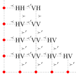
The idea of the algorithm is to build the shape $\pi$, one square at a time, starting from the empty partitions on the coordinate axes (red bullets in Figure 13), where at each square a partition is produced according to the type of the square.

Algorithm SchurSample
Input: $\pi$, partitions $\tau(0,0)=\tau(0,i)=\tau(j,0)=\emptyset$ and parameters $x_{i},y_{j}$, $1\leq i\leq m,1\leq j\leq n$
for $j=1\dots\ell(\pi)$
for $i=1\dots\pi_{j}$
$type$ = getType($i,j$)
$\tau(i,j)$=sample($\tau(i-1,j),\tau(i,j-1),\tau(i-1,j-1),x_{i}y_{j},type$)
Output: The sequence of partitions $\Lambda$ defined by

$$\Lambda:=(\emptyset=\tau(l_{0}),\tau(l_{1}),\dots,\tau(l_{m+n-1}),\tau(l_{m+n})=\emptyset),$$

where $(l_{0}=(0,n),l_{1},\dots,l_{m+n-1},l_{m+n}=(m,0))$ is the ordered sequence of lattice points on the boundary of $\pi$ clockwise from the vertical to the horizontal axis.

Our main result is then

Theorem 3.2.

The algorithm SchurSample produces an exact random sample from the Schur process corresponding to the word $w$ and the parameter list $Z$. This remains true if, in the algorithm, we replace the double for loop by any loop which runs over all the boxes $(i,j)$ of the encoded shape $\pi=sh(w)$ respecting their partial order (i.e. such that $\tau(i_{1},j_{1})$ is sampled before $\tau(i_{2},j_{2})$ if $i_{2}\geq i_{1}$ and $j_{2}\geq j_{1}$).

Proof.

Let $w$ be a word. Denote with $m$ the number of elements of $w$ in $\{\prec,\prec^{\prime}\}$ and with $n$ in $\{\prec,\prec^{\prime}\}$. We prove the statement is true for fixed $m$, $n$ and fixed parameter list $(X,Y)$ (obtained from $Z$ as described above). The proof is by induction on $|sh(w)|$. If $|sh(w)|=0$ then all $\{\succ,\succ^{\prime}\}$ come before $\{\prec,\prec^{\prime}\}$ and so the Schur process is supported on a single element, the sequence of empty partitions, which we sample trivially.

Suppose we can exactly sample a Schur process of $w$ for any word $w$ such that $|sh(w)|\leq k$. Let $w$ be a word with $|sh(w)|=k+1$. Then $w_{i}\in\{\prec,\prec^{\prime}\}$ and $w_{i+1}\in\{\succ,\succ^{\prime}\}$ for some $1\leq i<m+n$. Let $w^{0}$ be the word obtained from $w$ by interchanging elements at the $i$th and $i+1$-st position. Then $sh(w^{0})$ is obtained from $sh(w)$ by removing an outer corner and $|sh(w^{0})|=k$. By the inductive hypothesis we can sample this “smaller” process $\Lambda^{0}$ exactly (note that the parameter list $(X,Y)$ remains the same). We then perform an extra atomic step to add the missing corner to $sh(w^{0})$ to obtain $sh(w)$. That is, if $\lambda,\kappa,\mu$ are the three partitions that sit at the inner corner of $sh(w^{0})$ (like in Figure 10), we sample the outer corner $\nu$ based on the other three partitions using one of the four sample{HH,HV,VH,VV} procedures (chosen based on $(w_{i},w_{i+1})=(\prec,\succ),(\prec,\succ^{\prime}),(\prec^{\prime},\succ)$ or $(\prec^{\prime},\succ^{\prime}),$ respectively). The atomic step exactly samples this corner so that it fits into the new process correctly (everything depends only on the three partitions involved and the type of atomic step). Thus we obtain $\Lambda$ sampled exactly and correctly from $\Lambda^{0}$ by replacing (in $\Lambda^{0}$) the partition $\kappa$ with the partition $\nu$. ∎

Remark 3.3.

In the particular case of domino tilings of the Aztec diamond of size $n$, for which $w=(\prec^{\prime},\succ)^{n}$, our algorithm coincides with the domino shuffling algorithm [12, Section 6], provided that we grow the staircase partition $sh(w)=(n,n-1,\ldots,1)$ diagonal by diagonal. More precisely, we shall sample the $\tau(i,j)$ by increasing order of $i+j$, so that after $k(k+1)/2$ steps ($k=0,\ldots,n$), we have sampled the Schur process corresponding to the word $w^{(k)}=(\succ)^{n-k}(\prec^{\prime},\succ)^{k}(\prec^{\prime})^{n-k}$ hence to the encoded shape $sh(w^{(k)})=(k,k-1,\ldots,1,0,\ldots,0)$. This Schur process corresponds to tilings of the Aztec diamond of size $k$. Using the dimer interpretation of the sampleHV method shown in Figure 12, we see that the procedure for passing from $w^{(k)}$ to $w^{(k+1)}$ coincides with the domino shuffling bijection between diamonds of sizes $k$ and $k+1$. Let us mention that another description of the shuffling algorithm in terms of nonintersecting paths, equivalent to our particle/hole description, is given in [20].

Remark 3.4.

As is clear from the construction, any path going right and down from the vertical axis to the horizontal axis that appears in the construction of the Schur process encoded by $sh(w)$ (i.e., a subpartition of $sh(w)$ in Figure 3) will itself encode a Schur process. However, the process might not be related in a deeper way with the process encoded by $sh(w)$. For example, while $sh(w)$ may correspond to steep tilings, a subpartition of it may not. On the other hand, a subprocess on reverse plane partitions is also a reverse plane partition, or a staircase subprocess of the Aztec diamond is also an Aztec diamond.

Remark 3.5.

One can modify the algorithm slightly for better space complexity (but the same time complexity). At any time it is is enough to store $m+n+1$ partitions where $m=sh(w)_{1}$ and $n=\ell(sh(w))$. Indeed, one can start with the $m+n+1$ red dots depicting empty partitions in Figure 13 and sample using the local rules, but update partitions in place: that is, for example $\tau(1,1)$ would be sampled and then overwritten in the place of $\tau(0,0)$ since the latter is not needed anymore. Similarly $\tau(1,2)$ would be sampled and then overwritten in the place of $\tau(0,1)$ using the same logic, and so on.

The explicit description of the algorithm immediately allows us to estimate its time complexity, which is random and depends on the output. We assume that we can sample Bernoulli and geometric random variables in time $O(1)$. We have:

Proposition 3.6.

The time complexity of SchurSample is $O(|sh(w)|L)$, where we recall that $sh(w)$ is the encoding shape of the Schur process, and where $L:=\max\{\tau(l_{i})_{1},\ell(\tau(l_{i})),i\in[0\dots m+n]\}$ is the maximum of the maximum part and the maximum number of parts of the partitions in the output sequence $\Lambda$.

Proof.

This is clear by induction on $|sh(w)|$. Indeed, we have seen that the complexity of adding a box to $sh(w)$ (Cauchy case and dual Cauchy case) is $O(\max(\ell(\nu),\nu_{1}))$ where $\nu$ is the top-right partition in the added box, which is bounded by $O(L)$. ∎

Remark 3.7.

In some cases we can deterministically bound the quantity $L$ above, thus giving a deterministic, not output-sensitive, bound on the complexity. Suppose we sampled a Schur process of word $w$, and suppose that in doing so we never had to use both the sampleHH and the sampleVV procedure (this fact of course only depends on the word $w$). Plane partitions and Aztec diamonds are examples of such Schur processes. For simplicity, suppose we never had to use the sampleVV procedure (we may have used the sampleHH procedure multiple times though). Then under these assumptions, the time complexity of SchurSample is $O(|sh(w)|m)$ where $m$ is the total number of $\{\prec,\prec^{\prime}\}$ elements in $w$.

We now address entropy minimality/optimality. Consider a sample of the Schur process with word $w$ and encoded shape $sh(w)$. We claim that the random inputs needed to obtain it using SchurSample can be reconstructed. One simply has to proceed backwards, removing boxes from the encoded shape one at a time, and noting that the sample{HH,HV,VH,VV} methods can be reversed (since they are based on bijections) to recover the value of the geometric or Bernoulli random variable that they use. Thus we have:

Proposition 3.8.

Assuming that we can sample sequences of independent geometric random variables and random bits optimally, the algorithm SchurSample is entropy optimal.

Remark 3.9.

In the case of $(m\times n)$-boxed plane partitions (encoded shape is $m^{n}$), the SchurSample algorithm coincides with the RSK correspondence [13]. The latter takes an $m\times n$ array of nonnegative integers (corresponding to the values of the geometric random variables used in our algorithm) and maps it to a pair of semi-standard Young tableaux of common shape $\lambda$. One then takes these two tableaux and conjoins them (view each tableau as a sequence of interlacing partitions starting from $\emptyset$ and ending in $\lambda$) to obtain a plane partition (with central slice given by $\lambda$) which is the sampled plane partition.

Remark 3.10.

The algorithm above can be thus viewed as a generalized RSK correspondence. It takes a word $w$ and a partial matrix $(S_{ij})_{(i,j)\in sh(w)}$ of (geometric/Bernoulli) integers and produces a sequence of partitions which interlace or dually interlace at every step. It reduces to RSK as remarked above, but also to dual RSK, see also [13, 18, 25].

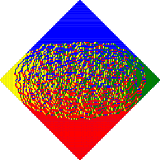
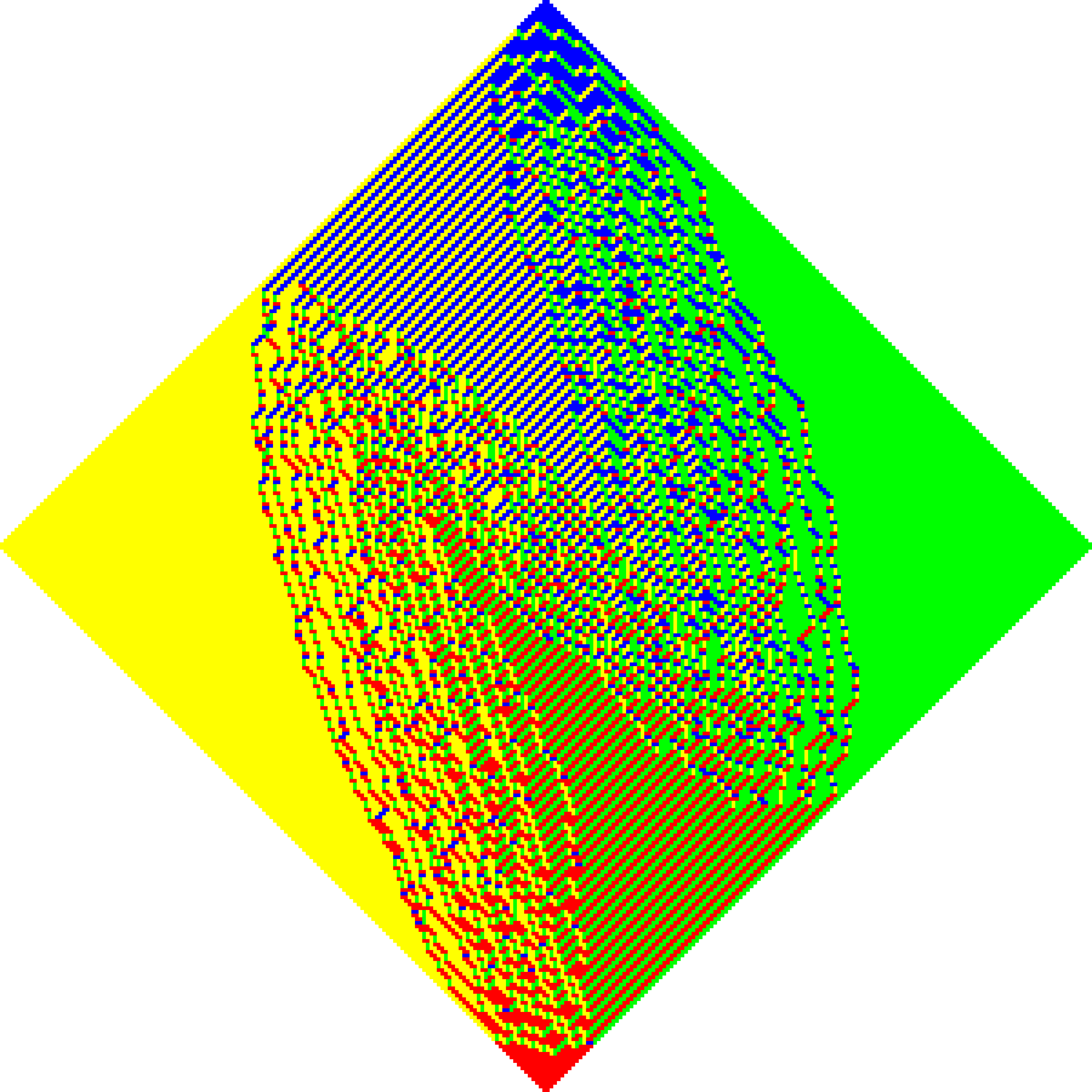
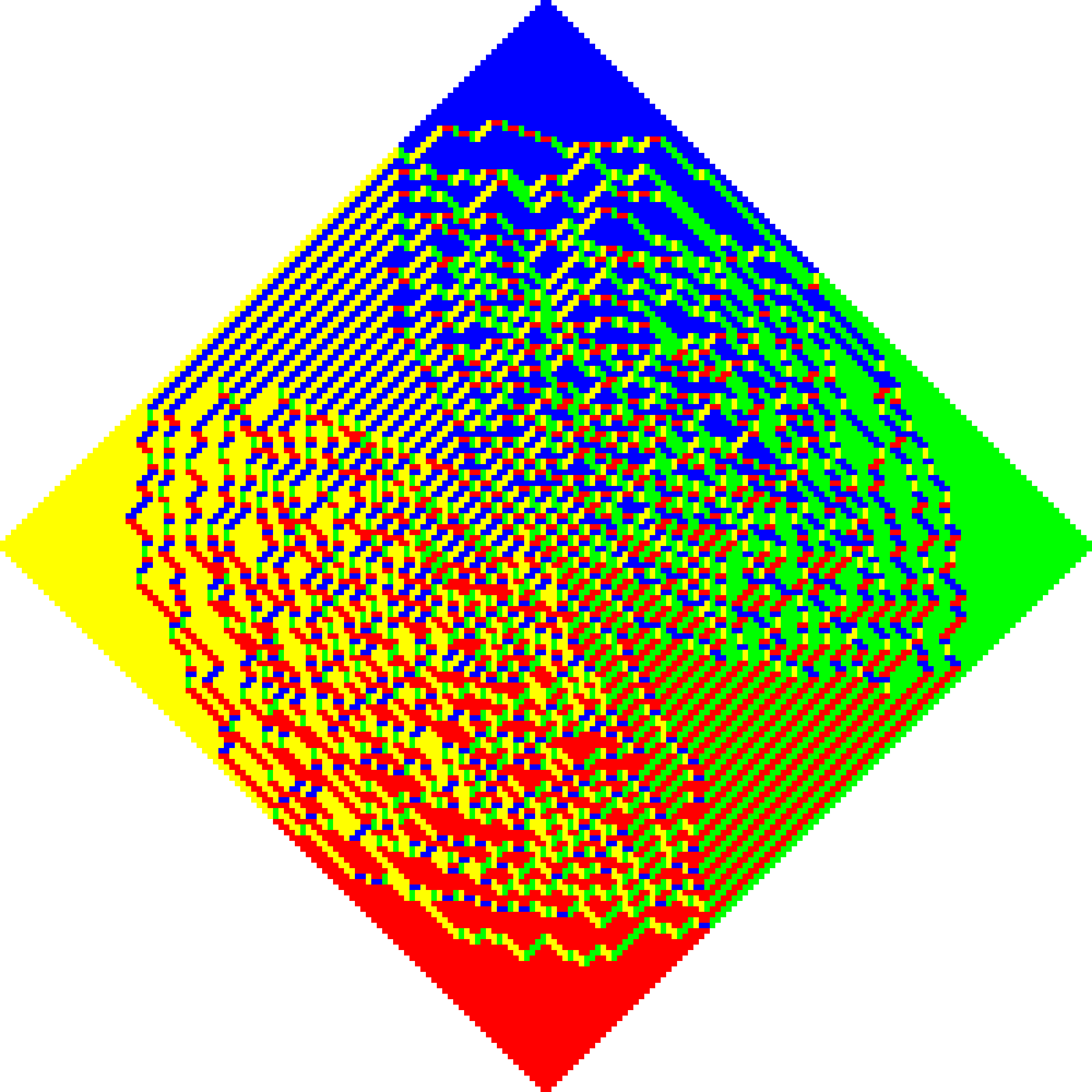
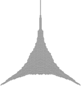
Below we present some samples using the given algorithm. In Figure 14 we present a large plane partition (a) and Aztec diamond (b). The deterministic asymptotic shape is a law of large numbers (see [23] for the case of the plane partition and [15] for the Aztec diamond). In Figure 15, we show a large pyramid partition. Its width and the parameter $q$ are tuned so that its apparent limit shape exhibits two interesting cusp points. Finally, in Figure 16 we present two large Aztec diamonds distributed according to a measure which is not the usual $q^{\text{Volume}}$. We can see (again) the appearance of cusps in the limit shape, as well as nodes (technically, two cusps coming “very close” to one another). This will be studied theoretically in future work.

(a)

(b)

Figure 14: A random large plane partition with base contained in a $100\times 100$ box and $q=0.93$ (a) and a random $100\times 100$ Aztec diamond with $q=0.99$ (b). Both exhibit deterministic limit shapes. The limit shape is known in the second case as the “arctic circle” (the terminology comes from the uniform case $q=1$, in which case the frozen boundary is indeed a circle).

Figure 15: A random pyramid partition of width $100$ with parameter $q=.99$ (only the particles of the corresponding Maya diagrams are displayed, not the dominoes). The apparent limit shape (in green) seems to exhibit cusp points (in blue), an interesting phenomenon that will be the subject of future work.

(a)

(b)

Figure 16: A random $150\times 150$ Aztec diamond with parameters $x_{2i-1}=48,x_{2i}=1/2,y_{2i-1}=16,y_{2i}=1/8,\ \forall i\geq 1$, exhibiting the formation of cusps (a), and a random $100\times 100$ Aztec diamond with parameters $x_{2i-1}=y_{2i-1}=20,x_{2i}=y_{2i}=1/20,\ \forall i\geq 1$ where the two cusps have coalesced (b).

4 Symmetric Schur processes

4.1 Basic definition and examples

We now turn our attention to Schur processes on interlaced sequences with a free boundary, i.e. where the end partition is not fixed. Precisely, for a word $w\in\{\prec,\succ,\prec^{\prime},\succ^{\prime}\}^{n}$ we will define the process on right-free $w$-interlaced sequence of partitions, i.e. $\Lambda=(\emptyset=\lambda(0),\lambda(1),\dots,\lambda(n))$ such that $\lambda(i-1)w_{i}\lambda(i)$, for $i=1,\dots,n$. This is a one-sided free boundary process, or mixed boundary process, since one side of the sequence is fixed (the empty partition), while the other one is free. One can, of course, define a double-sided free boundary Schur process, but we only provide a sampling algorithm for the one-sided free boundary process.

Definition 4.1.

For a word $w=(w_{1},w_{2},\dots,w_{n})\in\{\prec,\succ,\prec^{\prime},\succ^{\prime}\}^{n}$, the right-free Schur process of word $w$ with parameters $(Z;t)=(z_{1},\dots,z_{n};t)$ is the measure on the set of right-free $w$-interlaced sequences of partitions $\Lambda=(\emptyset=\lambda(0),\lambda(1),\dots,\lambda(n)=\lambda)$ given by

$$Prob(\Lambda)\propto t^{|\lambda_{n}|}\prod_{i=1}^{n}z_{i}^{||\lambda(i)|-|\lambda(i-1)||}.$$ (4.1)

Remark 4.2.

Note that we could have omitted the term with parameter $t$ and keep the full generality as the Schur process with parameter $(Z;t)$ is the same as the one with parameter $(\overline{Z};1)$ where $\overline{z}_{i}=t^{\epsilon_{i}}z_{i}$ and $\epsilon_{i}=1$ if $w_{i}\in\{\prec,\prec^{\prime}\}$ and $-1$ otherwise, for $i=1,\dots,n$.

We will also here refer to the right-free Schur process as a symmetric Schur process since it can be defined as a measure on symmetric sequences of length $2n+1$ starting and ending with the empty partition, i.e.

$$(\emptyset=\lambda(0),\lambda(1),\dots,\lambda(n-1),\lambda(n)=\lambda,\lambda(n-1),\dots,\lambda(1),\lambda(0)=\emptyset)$$ (4.2)

with probability proportional to

$$\prod_{i=1}^{2n+1}t_{i}^{||\lambda(i)|-|\lambda(i-1)||}$$ (4.3)

where $t_{i}t_{2n-i+1}=t^{\epsilon_{i}}z_{i}$, for $i=1,\dots,n$.

We now give examples of right-free (or symmetric) interlaced sequences on which the Schur process described above can be defined. These examples correspond to symmetric tilings of a plane.

Symmetric reverse plane partitions

of symmetric shape $\mathcal{S}$, are reverse plane partitions of shape $\mathcal{S}$ with symmetric fillings, i.e. $\pi_{i,j}=\pi_{j,i}$. Of course we assume the shape $\mathcal{S}$ to be symmetric, namely that $(i,j)\in\mathcal{S}$ implies $(j,i)\in\mathcal{S}$. They are in bijection with symmetric $w$-interlaced sequences where $sh(w)=\mathcal{S}$. Special case when $\mathcal{S}$ is the Young diagram of $n^{n}$ corresponds to symmetric $(n\times n)$-boxed plane partitions. Symmetric reverse plane partitions correspond to symmetric planar lozenge tilings.

Plane overpartitions

[9] and, more generally, one-sided free boundary steep tilings [7] are examples of right-free (or equivalently symmetric) domino tilings of a plane. A plane overpartition is a plane partition where in each row the last occurrence of an integer can be overlined or not and all the other occurrences of this integer are not overlined, also in each column the first occurrence of an integer can be overlined or not and all the other occurrences of this integer are overlined. An example of a plane overpartition is given in Figure 17.

Figure 17: A plane overpartition partition corresponding to the interlacing sequence $\emptyset\prec(1)\prec^{\prime}(2)\prec(2,2)\prec^{\prime}(3,3,1)\prec(5,3,1)\prec^{\prime}(5,4,1)\prec(5,4,1,1)\prec^{\prime}(5,4,2,1)$.

Plane overpartitions whose largest filling is at most $n$ are in correspondence with right-free $w$-interlaced sequences where $w=(\prec,\prec^{\prime})^{n}$. Indeed, starting from a plane partition of shape $\lambda$ with the largest part at most $n$ we can form a sequence of interlaced partitions

$$\emptyset=\lambda(0)\prec\lambda(1)\prec^{\prime}\lambda(2)\prec\cdots\prec\lambda(2n-1)\prec^{\prime}\lambda(2n)=\lambda$$

where $\lambda(i)$ is the partition whose shape is formed by all fillings greater than ${n-i/2}$, where the convention is that $\overline{k}=k-1/2$. From this it is clear that they can also be viewed as symmetric pyramid partitions.

Plane overpartitions are a special case of a one-sided free boundary steep tilings, i.e. domino tilings which are in correspondence with right-free $w$-interlaced sequences where $w_{2i}\in\{\prec,\succ\}$ and $w_{2i+1}\in\{\prec^{\prime},\succ^{\prime}\}$. See [7] for details.

4.2 Sampling algorithm

We now give the exact sampling algorithm for the symmetric Schur process of word $w$ with parameters $(Z;1)$. The algorithm is a modification of SchurSample.

Let $w^{sym}=w\cdot w^{*}$, where $w^{*}$ is obtained by reversing the word $w$ first and then by inverting every element in the word, where by inverting we mean replacing $\succ$ (respectively $\succ^{\prime}$) with $\prec$ (respectively $\prec^{\prime}$), and vice versa. Also, let $Z^{sym}=Z\cdot Z^{r}$ where $Z^{r}$ is the reverse of $Z$. For example, for the word $w=(\prec,\succ^{\prime})$ and $Z=(z_{1},z_{2})$, $w^{sym}=(\prec,\succ^{\prime},\prec^{\prime},\succ)$ and $Z^{sym}=(z_{1},z_{2},z_{2},z_{1})$. Set $(\pi,X,Y,\text{getType})={{\tt Par}}(w^{sym},Z^{sym})$ where $\tt{Par}$ is defined in the pre-computation step of $\tt{SchurSample}$. Note that in this case the number of $x$’s and $y$’s is the same and equal to the length of the word $w$, say $n$, and that $x_{i}=y_{i}$, for $i=1,\dots,n$.

The algorithm that produces samples form the symmetric Schur process is obtained from SchurSample for word $w^{sym}$ and parameters $Z^{sym}$ with the following two alternations. Since the output needs to be symmetric, at each step we need to make sure that the partitions corresponding to off-diagonal boxes $(i,j)$ and $(j,i)$ are equal. This just means that we need to add two boxes to the symmetric shape at the same time and use the same sample for both boxes to construct the corresponding partition. The sample will come from either $Geom(x_{i}y_{j})$ or $Bernoulli(x_{i}y_{j})$ depending on the type of the box $(i,j)$. Another difference is that the partitions corresponding to the diagonal boxes $(i,i)$ will be constructed using a sample from $Geom(x_{i})=Geom(\sqrt{x_{i}y_{i}})$. The algorithm is given below.

Algorithm SymmetricSchurSample
Input: $\pi$, partitions $\tau(0,i)=\emptyset=\tau(j,0)$ and parameters $x_{i}=y_{i}$, $0\leq i,j\leq n$
for $j=1\dots\ell(\pi)$
for $i=1\dots\pi_{j}$
if $j>i$
$type$ = getType($i,j$)
$\tau(i,j)$=sample($\tau(i-1,j),\tau(i,j-1),\tau(i-1,j-1),x_{i}y_{j},type$)
elseif $j==i$
$type$ = getType($i,i$)
$\tau(i,i)$=sample($\tau(i-1,i),\tau(i-1,i),\tau(i-1,i-1),x_{i},type$)
elseif $j<i$
$\tau(i,j)=\tau(j,i)$
Output: The sequence of partitions $\Lambda$ defined by

$$\Lambda:=(\emptyset=\tau(l_{0}),\tau(l_{1}),\dots,\tau(l_{n})=\lambda,\dots,\tau(l_{2n-1})=\tau(l_{1}),\tau(l_{2n})=\tau(l_{0})=\emptyset),$$

where $(l_{0}=(0,n),l_{1},\dots,l_{2n-1},l_{2n}=(n,0))$ is the ordered sequence of lattice points on the boundary of $\pi$ clockwise from the vertical to the horizontal axis.

Note that the diagonal elements in the algorithm above are produced either using sampleHH or sampleVV procedure where $\lambda=\mu$ in the notation given in the description of the bijections. So, they are produced using the following bijection $(\kappa,G)\mapsto\nu$ where

$$\nu_{i}=\begin{cases}\mu_{1}+G&\text{if $i=1$},\\ \mu_{i}+\mu_{i-1}-\kappa_{i-1}&\text{if $i>1$}.\\ \end{cases}$$ (4.4)

This is a bijective mapping from $\mu$ and $G\in\mathbb{N}$ such that $\mu\succ\kappa$ to $\nu$ such that $\mu\prec\nu$, for a fixed $\mu$. In addition, we have that $2|\mu|+G=|\kappa|+|\nu|$. Thus, the diagonal elements of type HH are produced using
def sampleH($\mu,\kappa,x$)
sample $G\sim Geom(x)$
construct $\nu$ as in (4.4)
return $\nu$
The diagonal elements of type VV are obtained by conjugating sampleH($\mu^{\prime},\kappa^{\prime},x$). The bijection described above allow us to prove the Littlewood identity [19, p. 93]

$$\sum_{\nu}s_{\nu/\mu}(X)=\prod_{i}\frac{1}{1-x_{i}}\prod_{i<j}\frac{1}{1-x_{i}x_{j}}\sum_{\kappa}s_{\mu/\kappa}(X),$$

or, equivalently, the reflection relations [7]

$$\Gamma_{+}(z)|\underline{t}\rangle =\frac{1}{1-zt}\Gamma_{-}(zt^{2})|\underline{t}\rangle,$$ (4.5)

$$\tilde{\Gamma}_{+}(z)|\underline{t}\rangle =\frac{1}{1-zt}\tilde{\Gamma}_{-}(zt^{2})|\underline{t}\rangle,$$ (4.6)

where

$$|\underline{t}\rangle=\sum_{\nu}t^{|\nu|}|\nu\rangle.$$ (4.7)

The proof follows from:

$$\sum_{\begin{subarray}{c}\nu\\ \mu\prec\nu\end{subarray}}z^{|\nu|-|\mu|}t^{|\nu|}=\sum_{\begin{subarray}{c}\kappa\\ \mu\succ\kappa\end{subarray}}\sum_{G\geq 0}z^{|\mu|-|\kappa|+G}t^{2|\mu|-|\kappa|+G}=\frac{1}{1-zt}\sum_{\begin{subarray}{c}\kappa\\ \mu\succ\kappa\end{subarray}}(zt^{2})^{|\mu|-|\kappa|}t^{|\kappa|}.$$ (4.8)

The partition function of the symmetric Schur process can then be written as:

$$Z^{sym}_{w}=\sum_{\Lambda}t^{|\lambda(n)|}\prod_{i=1}^{n}z_{i}^{||\lambda(i)|-|\lambda(i-1)||}=\langle\emptyset|\prod_{i=1}^{n}\Gamma_{i}(z_{i})|\underline{t}\rangle,$$ (4.9)

where $\Gamma_{i}$ is defined as before, i.e. it is $\Gamma_{+},\Gamma_{-},\tilde{\Gamma}_{+},\tilde{\Gamma}_{-}$ if $w_{i}$ is $\prec,\succ,\prec^{\prime},\succ^{\prime}$, respectively.

Using the commutation relation, reflection relations and action of $\Gamma$’s on the vacuum vectors we get the following proposition.

Proposition 4.3.

The partition function of the right-free Schur process of word $w$ with parameters $(Z;t)$ is

$$Z_{w}^{symm}=\prod_{i,w_{i}\in\{\prec,\prec^{\prime}\}}\frac{1}{1-tz_{i}}\prod_{i<j,w_{i}\in\{\prec,\prec^{\prime}\},w_{j}\in\{\succ,\succ^{\prime}\}}(1+\epsilon_{i,j}z_{i}z_{j})^{\epsilon_{i,j}}\prod_{i<j,w_{i},w_{j}\in\{\prec,\prec^{\prime}\}}(1+\delta_{i,j}t^{2}z_{i}z_{j})^{\delta_{i,j}}$$ (4.10)

where $\epsilon_{i,j}=1$ if $(w_{i},w_{j})\in\{(\prec,\succ^{\prime}),(\prec^{\prime},\succ)\}$ and $\epsilon_{i,j}=-1$ otherwise, $\delta_{i,j}=-1$ if $w_{i}=w_{j}$ and $\delta_{i,j}=1$ otherwise.

4.3 Even row and even column symmetric Schur processes

One can introduce versions of the symmetric Schur process by requesting that the free partition has all even parts or that its conjugate has even parts. We call these the even rows and even columns symmetric Schur processes.

One can derive the partition functions for such processes using the Cauchy identities and the modified versions of the Littlewood identity [19, p. 93]

$$\sum_{\nu\ \text{with even rows}}s_{\nu/\mu}(X) =\prod_{i\leq j}\frac{1}{1-x_{i}x_{j}}\sum_{\kappa\ \text{with even rows}}s_{\mu/\kappa}(X),$$ (4.11)

$$\sum_{\nu\ \text{with even columns}}s_{\nu/\mu}(X) =\prod_{i<j}\frac{1}{1-x_{i}x_{j}}\sum_{\kappa\ \text{with even columns}}s_{\mu/\kappa}(X).$$ (4.12)

They are equivalent to the reflection relations [7]

$$\Gamma_{+}(z)|\underline{t}^{er}\rangle =\frac{1}{1-(zt)^{2}}\Gamma_{-}(zt^{2})|\underline{t}^{er}\rangle,$$ (4.13)

$$\tilde{\Gamma}_{+}(z)|\underline{t}^{er}\rangle =\tilde{\Gamma}_{-}(zt^{2})|\underline{t}^{er}\rangle,$$ (4.14)

$$\Gamma_{+}(z)|\underline{t}^{ec}\rangle =\Gamma_{-}(zt^{2})v^{ec}(t),$$ (4.15)

$$\tilde{\Gamma}_{+}(z)|\underline{t}^{ec}\rangle =\frac{1}{1-(zt)^{2}}\tilde{\Gamma}_{-}(zt^{2})|\underline{t}^{ec}\rangle,$$ (4.16)

where

$$|\underline{t}^{er}\rangle=\sum_{\nu\ \text{with even rows}}t^{|\nu|}|\nu\rangle\quad\text{and}\quad|\underline{t}^{ec}\rangle=\sum_{\nu\ \text{with even columns}}t^{|\nu|}|\nu\rangle.$$ (4.17)

Proposition 4.4.

The partition functions for the even rows/columns symmetric Schur processes read

$$Z_{w}^{symm,\ er} =\prod_{i,w_{i}=\prec}\frac{1}{1-(tz_{i})^{2}}\prod_{i<j,w_{i}\in\{\prec,\prec^{\prime}\},w_{j}\in\{\succ,\succ^{\prime}\}}(1+\epsilon_{i,j}z_{i}z_{j})^{\epsilon_{i,j}}\prod_{i<j,w_{i},w_{j}\in\{\prec,\prec^{\prime}\}}(1+\delta_{i,j}t^{2}z_{i}z_{j})^{\delta_{i,j}},$$ (4.18)

$$Z_{w}^{symm,\ ec} =\prod_{i,w_{i}=\prec^{\prime}}\frac{1}{1-(tz_{i})^{2}}\prod_{i<j,w_{i}\in\{\prec,\prec^{\prime}\},w_{j}\in\{\succ,\succ^{\prime}\}}(1+\epsilon_{i,j}z_{i}z_{j})^{\epsilon_{i,j}}\prod_{i<j,w_{i},w_{j}\in\{\prec,\prec^{\prime}\}}(1+\delta_{i,j}t^{2}z_{i}z_{j})^{\delta_{i,j}}$$ (4.19)

where $\epsilon_{i,j}=1$ if $(w_{i},w_{j})\in\{(\prec,\succ^{\prime}),(\prec^{\prime},\succ)\}$ and $\epsilon_{i,j}=-1$ otherwise, $\delta_{i,j}=-1$ if $w_{i}=w_{j}$ and $\delta_{i,j}=1$ otherwise.

SymmetricSchurEvenRowsSample and SymmetricSchurEvenColumnsSample algorithms are obtained from SymmetricSchurSample by changing the sampling of diagonal elements, i.e. by changing sampleH and sampleV. We start with the even row case. We need to make minor changes to make sure we produce even partitions, i.e. partitions with even rows. In this case we need a bijection that maps pairs of even partitions $\kappa$, where $\mu\succ\kappa$, and $G\in\mathbb{N}$ to even partitions $\nu$ such that $\mu\prec\nu$. We can achieve this by setting

$$\nu_{i}=\begin{cases}2\lceil\mu_{1}/2\rceil+2G&\text{if $i=1$},\\ 2\lceil\mu_{i}/2\rceil+2\lfloor\mu_{i-1}/2\rfloor-\kappa_{i-1}&\text{if $i>1$}.\\ \end{cases}$$ (4.20)

The bijection satisfies $2|\mu|+2G=|\kappa|+|\nu|$ and can be used to prove the Littlewood identity (4.11) or equivalently (4.13) and (4.14). SymmetricSchurEvenRowsSample is obtained from SymmetricSchurSample by replacing sampleH with sampleH^er:
def sampleH^er($\mu,\kappa,x$)
sample $G\sim Geom(x^{2})$
construct $\nu$ as in (4.20)
return $\nu$

For the even column case, we need a bijection that maps even column partitions $\kappa$, where $\mu\succ\kappa$ to even column partitions $\nu$ such that $\mu\prec\nu$. We can achieve this by setting

$$\nu_{i}=\begin{cases}\mu_{1}&\text{if $i=1$},\\ \mu_{i}+\mu_{i-1}-\kappa_{i-1}&\text{if $i>1$}.\\ \end{cases}$$ (4.21)

The bijection satisfies $2|\mu|=|\kappa|+|\nu|$ and can be used to prove the Littlewood identity (4.12) or equivalently (4.15) and (4.16). In this case we replace sampleH with sampleH^ec:
def sampleH^ec($\mu,\kappa,x$)
construct $\nu$ as in (4.21)
return $\nu$

Note that sampleH^ec is deterministic since in this case we do not need to produce a random number $G$, as in previous cases.

Remark 4.5.

Correctness, complexity analysis and the entropy optimality of the regular SchurSample algorithm transfer, mutatis mutandis, to the symmetric cases.

Remark 4.6.

Our sampling algorithm is based on an RSK-type correspondence between symmetric $w^{sym}$-interlaced sequences and symmetric fillings of $sh(w^{sym})$. Depending on the type of the box, the fillings are either nonnegative integers or elements of $\{0,1\}$. Each box $(i,j)$, where $i\leq j$ has a corresponding term in the partition function. The three groups of terms, see Proposition 4.3, correspond to three groups of boxes (diagonal boxes, the upper part of $\pi$ corresponding to the encoded shape of $w$, and the group of all other boxes i.e., below the second group and to the left of the diagonal boxes). Even row or even column cases are similar except we use different bijections for diagonal boxes and in the even column case all diagonal boxes are filled with zeros. The three algorithms for sampling symmetric Schur processes described above can be viewed as generalizations of the symmetric RSK [17, 28].

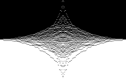
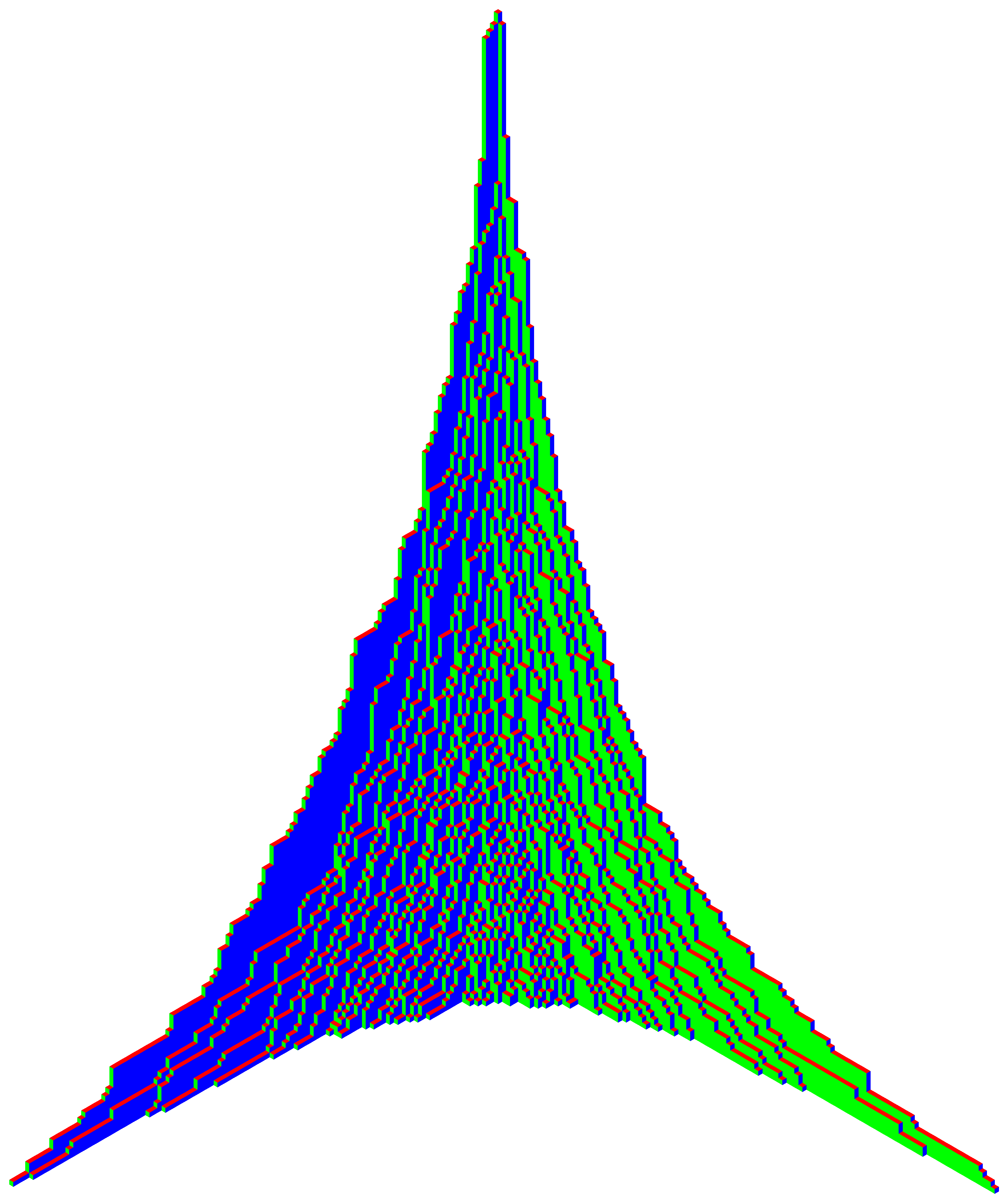
In Figure 18 we present, side by side, the output of sampling a plane partition with parameter $q=0.953$ and a symmetric plane partition with parameter $q_{s}=q^{2}$. The two outputs are clearly comparable and one observes a similarity in the limit shapes, but note that the two $q$ parameters are related to each other by squaring (this is accounted for by the fact that we are sampling “half” as many geometric random variables in the symmetric case compared to the non-symmetric case). In Figure 19 we present the particle configuration associated to an unbounded symmetric pyramid partition with parameter $q=0.95$ and the plot (as a plane partition) of the associated plane overpartition tableau (see example in Figure 17), after the mapping $\overline{i}\mapsto 2i-1,i\mapsto 2i$. Note the plane partition is a strict plane partition in the terminology of [29].

(a)

(b)

Figure 18: A random plane partition for $q=0.953$ (a) and a random symmetric plane partition for $q^{2}$ (b).

(a)

(b)

Figure 19: An unbounded symmetric pyramid partition (only particles and holes depicted) (a) and the height function (as a plane partition) of the plane overpartition coming from (half) the associated symmetric Schur process (b), after we have replaced $\overline{i}\mapsto 2i-1,i\mapsto 2i$ in the tableau.

5 Schur processes with infinitely many parameters

In Definition 2.1 we consider Schur processes depending on a finite number of parameters: a finite word $w$ defining the interlacing relations, and a sequence of weights $Z$ controlling the size variation of the partitions. This is not the most general definition of a Schur process as, for instance, one could consider infinite sequences of interlaced partitions such as those coding for (unboxed) plane partitions [23]. In this section we explain how to handle such a situation, and the most general Schur process will be discussed in the next section.

For simplicity we will concentrate on the case of a bi-infinite sequence of partitions $\Lambda=(\lambda(i))_{i\in\mathbb{Z}}$ forming a “pyramid” in the sense that

$$\begin{cases}\lambda(i)\succ\lambda(i+1)\text{ or }\lambda(i)\succ^{\prime}\lambda(i+1)&\text{for $i\geq 0$,}\\ \lambda(i)\succ\lambda(i-1)\text{ or }\lambda(i)\succ^{\prime}\lambda(i-1)&\text{for $i\leq 0$,}\\ \lambda(i)=\emptyset&\text{for $|i|$ large enough.}\end{cases}$$ (5.1)

In the terminology of Section 2, we are considering a $w$-interlaced sequence of partitions where $w$ is bi-infinite word where no $\prec$ or $\prec^{\prime}$ appears on the right of a $\succ$ or $\succ^{\prime}$. This situation includes unboxed plane partitions (when we have only unprimed symbols) and pyramid partitions of arbitrary width (when primed and unprimed symbols alternate). To each sequence satisfying (5.1), we associate a weight

$$W(\Lambda)=\prod_{i\geq 0}a_{i}^{|\lambda(-i)|-|\lambda(-i-1)|}\prod_{j\geq 0}b_{j}^{|\lambda(j)|-|\lambda(j+1)|}$$ (5.2)

where the $a$’s and $b$’s are nonnegative real parameters. The most natural specialization is again the $q^{\text{Volume}}$ measure which is here obtained for instance by taking $a_{i}=b_{i}=q^{i+1/2}$ for all $i\geq 0$. By adapting Proposition 2.3, it is straightforward to check that the partition function reads

$$Z_{w}=\prod_{i,j\geq 0}(1+\epsilon_{i,j}a_{i}b_{j})^{\epsilon_{i,j}},$$ (5.3)

where $\epsilon_{i,j}=1$ if $(w_{-i},w_{j+1})\in\{(\prec,\succ^{\prime}),(\prec^{\prime},\succ)\}$ and $\epsilon_{i,j}=-1$ otherwise. It is finite whenever

$$\sum_{i\geq 0}(a_{i}+b_{i})<\infty,$$ (5.4)

so that normalizing (5.2) yields a probability measure over sequences satisfying (5.1), which we call the pyramidal Schur process of parameters $(a_{i},b_{i})_{i\geq 0}$. Note that the marginal law of $\lambda(0)$ is a Schur measure [22].

Our goal is to describe a perfect sampling algorithm for the pyramidal Schur process (and thus for the Schur measure). Conceptually speaking, it consists in sampling an infinite collection of independent geometric or Bernoulli random variables that has finite support, then applying our RSK-type correspondence. Let us present this in our algorithmic setting. Observe that, when we truncate the weight sequences, i.e. when we set $a_{i}=b_{i}=0$ for $i\geq M$, then $\lambda(i)=\emptyset$ for $|i|\geq M$ and we are back to the finite setting, so that we may apply the SchurSample finite algorithm. Roughly speaking our generalized algorithm consists in first sampling a suitable $M$ then applying the finite algorithm modified so as to remove the bias.

More precisely, in the truncated setting, the SchurSample algorithm receives as input the encoded shape $\pi_{M}=M^{M}$ (i.e. a $M\times M$ square) and the parameters $X=(x_{1},\ldots,x_{M})=(a_{M-1},\ldots,a_{0})$ and $Y=(y_{1},\ldots,y_{M})=(b_{M-1},\ldots,b_{0})$. Recall that generating the partition $\tau(i,j)$ corresponding to the box $(i,j)$ of $\pi_{M}$ involves sampling, independently of all the other boxes, a geometric or Bernoulli random variable with parameter depending on $x_{i}y_{j}=a_{M-i}b_{M-j}$. It is convenient to perform the change of coordinates $(i,j)\to(M-i,M-j)$ so that to the law of the random variable $U_{i,j}$ attached to the box $(i,j)$ does not depend on $M$, as long as $i,j<M$. Note that, in the new coordinates, we now generate the $\tau(i,j)$ in decreasing partial order of $(i,j)$, starting with the boundary conditions $\tau(M,j)=\tau(i,M)=\emptyset$. The law of $U_{i,j}$ ($0\leq i,j<M$) reads explicitly

$$U_{i,j}\sim\begin{cases}Geom(c_{i,j})&\text{where $c_{i,j}=a_{i}b_{j}\phantom{/(1+a_{i}b_{j})}$ if $\epsilon_{i,j}=-1$,}\\ Bernoulli(c_{i,j})&\text{where $c_{i,j}=a_{i}b_{j}/(1+a_{i}b_{j})$ if $\epsilon_{i,j}=1$.}\end{cases}$$ (5.5)

By a natural coupling, we may realize all values of $M$ on the same probability space, so that $U_{i,j}$ ($i,j\geq 0$) is a random variable independent of $M$. Using (5.4) and the Borel-Cantelli lemma, it is not difficult to check that, almost surely, only finitely many $U_{i,j}$ are nonzero. Therefore there exists $M$ such that $U_{i,j}=0$ unless $0\leq i,j<M$, and it can be seen that the output of the truncated algorithm does not depend on $M$ provided it satisfies this condition.

Rather than sampling $M$ itself, it is convenient to reduce the problem to a unidimensional one by labeling the boxes by a single integer. A convenient choice is to label the boxes using the Cantor pairing function $k(i,j)=(i+j)(i+j+1)/2+j$ which defines a bijection $\mathbb{N}\times\mathbb{N}\to\mathbb{N}$ ($k(0,0)=0$, $k(1,0)=1$, $k(0,1)=2$, $k(2,0)=3\dots$). Setting $K=\sup\{k(i,j):i,j\geq 0\text{ and }\ U_{i,j}>0\}$, we have

$$\mathbb{P}(K\leq k)=\prod_{\begin{subarray}{c}i,j\geq 0\\ k(i,j)>k\end{subarray}}(1-c_{i,j})$$ (5.6)

which is positive by (5.4) and tends to $1$ as $k\to\infty$. This explicit expression makes it theoretically possible to sample $K$, for instance by drawing a uniform real (Lebesgue) random variable $V$ on $[0,1]$ and taking the largest $k$ such that $\mathbb{P}(K\leq k)<V$. Discussing a practical perfect algorithm to do that on a real-world computer is beyond the scope of this paper, though this could be conceivably done by computing sufficiently good bounds for the right hand side of (5.6) and sampling enough digits in the binary expansion of $V$. Let us mention by the way that the mere efficient sampling of geometric random variables of arbitrary parameter on a real-world computer is already a nontrivial task [8].

Conditionally on $\{K=k\}$, the distribution of the $U_{i,j}$ is easy to describe: all $U_{i,j}$ with $k(i,j)>k$ are zero, all $U_{i,j}$ with $k(i,j)<k$ remain distributed as in (5.5), and if $k=k(i,j)$ then $U_{i,j}=1$ if $\epsilon_{i,j}=1$ and $U_{i,j}\sim 1+Geom(c_{i,j})$ if $\epsilon_{i,j}=-1$. Once we have generated the random inputs, we then generate the partitions $\tau(i,j)$ in a way similar to before. We summarize this discussion in the following pseudocode and proposition.

Algorithm UnboundedSchurSample
Input: parameters $a_{i}$ and $b_{i}$, $i\geq 0$
initialize a sparse partition-valued matrix $\tau(i,j)=\emptyset$ for all $i,j\geq 0$
sample $K$ distributed as (5.6)
if $K==-\infty$: return empty Schur process
find $(i_{0},j_{0})$ such that $K=k(i_{0},j_{0})$, $n_{0}=i_{0}+j_{0}$
case getType($i_{0},j_{0}$):
(HV$|$VH): $\tau(i_{0},j_{0})=1$
HH: $\tau(i_{0},j_{0})=1+Geom(a_{i_{0}}b_{i_{0}})$
VV: $\tau(i_{0},j_{0})=(1+Geom(a_{i_{0}}b_{i_{0}}))^{\prime}$
for $n=n_{0}\dots 1$
for $j=0\dots n$
if $n==n_{0}$ and $j\geq j_{0}$: next
$type$ = getType($n_{0}-j,j$)
$\tau(i,j)$=sample($\tau(i+1,j),\tau(i,j+1),\tau(i+1,j+1),a_{i}b_{j},type$)
Output: The sequence of partitions $\lambda(i)$, $i\in\mathbb{Z}$, defined by

$$\lambda(i):=\begin{cases}\tau(-i,0)\text{ if $i<0$, }\\ \tau(0,i)\text{ otherwise.}\end{cases}$$

Proposition 5.1.

The output of the algorithm UnboundedSchurSample is distributed as the pyramidal Schur process of parameters $(a_{i},b_{i})_{i\geq 0}$.

Our algorithm can be straightforwardly adapted to infinite sequences of partitions satisfying more general interlacing conditions than (5.1), and also to free or periodic [1] boundary conditions. Indeed, in all these models, the partition function is equal to a convergent infinite product [7], and there exists a RSK-type bijection which maps the process to a countable collection of independent geometric or Bernoulli random variables whose support is almost surely finite, and which can be sampled using a similar strategy.

6 General Schur processes with exponential specializations

In this section we sketch how to sample the most general Schur process [23, 2], defined as a measure over sequences $\Lambda$ of integer partitions of the form

$$\emptyset\subset\lambda(1)\supset\mu(1)\subset\lambda(2)\supset\mu(2)\subset\cdots\supset\mu(N-1)\subset\lambda(N)\subset\emptyset$$ (6.1)

where the probability of a given sequence is given by

$$Prob(\Lambda)\propto s_{\lambda(1)}(\rho_{0}^{+})s_{\lambda(1)/\mu(1)}(\rho_{1}^{-})s_{\lambda(2)/\mu(1)}(\rho_{1}^{+})\cdots s_{\lambda(N)/\mu(N-1)}(\rho_{N-1}^{+})s_{\lambda(N)}(\rho_{N}^{-}).$$ (6.2)

Here the parameters $\rho_{i}^{+}$ ($i=0,\ldots,N-1$) and $\rho_{i}^{-}$ ($i=1,\ldots,N$) are nonnegative specializations of the algebra of symmetric functions, which means that there exist countable collections of nonnegative real parameters $\alpha^{\pm}_{i,k}$ and $\beta^{\pm}_{i,k}$ ($k\geq 1$), and nonnegative real parameters $\gamma_{i}^{\pm}$, such that

$$\sum_{k\geq 1}(\alpha^{\epsilon}_{i,k}+\beta^{\epsilon}_{i,k})<\infty$$ (6.3)

for all $i$ and $\epsilon\in\{+,-\}$, and

$$H(\rho_{i}^{\epsilon};u):=\sum_{n=0}^{\infty}h_{n}(\rho_{i}^{\epsilon})u^{n}=e^{\gamma_{i}^{\epsilon}u}\prod_{k\geq 1}\frac{1+\beta^{\epsilon}_{i,k}u}{1-\alpha^{\epsilon}_{i,k}u}.$$ (6.4)

This indeed suffices to determine the values of the (skew) Schur functions appearing in (6.2) via (2.3) and (2.4).

Definition 2.1 corresponds to the situation where all parameters $\gamma_{i}^{\pm}$ are zero, and only a finite number of parameters $\alpha^{\pm}_{i,k}$ and $\beta^{\pm}_{i,k}$ are nonzero. Indeed, assuming that $\alpha^{\pm}_{i,k}=\beta^{\pm}_{i,k}$ for $k>M$, we have

$$\begin{split}s_{\lambda/\mu}(\rho^{\epsilon}_{i})&=\sum_{\nu:\mu\subset\nu\subset\lambda}s_{\nu/\mu}(\alpha^{\epsilon}_{i,1},\ldots,\alpha^{\epsilon}_{i,M})s_{\lambda^{\prime}/\nu^{\prime}}(\beta^{\epsilon}_{i,1},\ldots,\beta^{\epsilon}_{i,M})\\ &=\langle\mu|\Gamma_{+}(\alpha^{\epsilon}_{i,1})\cdots\Gamma_{+}(\alpha^{\epsilon}_{i,M})\tilde{\Gamma}_{+}(\beta^{\epsilon}_{i,1})\cdots\tilde{\Gamma}_{+}(\beta^{\epsilon}_{i,M})|\lambda\rangle\end{split}$$ (6.5)

which may be readily expanded as a sum over finite sequences of interlaced partitions, as in our original definition. (To make the connection precise we shall take $n=4MN$, $w=(\prec^{M}\prec^{\prime M}\succ^{M}\succ^{\prime M})^{N}$ and get the parameters $Z$ by listing all the parameters $\alpha$ and $\beta$ in a suitable order. Note that, in Definition 2.1, we may assume without loss of generality $w$ to be of this form, upon taking some $z_{i}$’s to be zero hence forcing some pairs of successive partitions to be equal.)

If we lift the restriction that only a finite number of parameters $\alpha^{\pm}_{i,k}$ and $\beta^{\pm}_{i,k}$ are nonzero, but keep the restriction that all the $\gamma_{i}^{\pm}$ vanish, then we may produce a perfect sample of the Schur process following the strategy of Section 5, which treats the case $N=1$, but can be easily adapted to general $N$.

Therefore, to sample the most general Schur process, our only missing ingredient is an algorithm to handle the $\gamma$ parameters, that correspond to exponential specializations. For simplicity we again treat only the case $N=1$ (that is to say we only need to sample a single partition whose law is a Schur measure) with $\rho_{0}^{+}$ a “pure” exponential specialization (i.e. $\alpha_{0,k}^{+}=\beta_{0,k}^{+}=0$ for all $k\geq 1$) and $\rho_{1}^{-}$ either another pure exponential specialization (Plancherel case) or a specialization with $\gamma_{1}^{-}=0$ (mixed case). The adaptation to the most general situation is left to the reader.

For any fixed skew shape $\lambda/\mu$, we have the well-known identity [28]

$$\lim_{n\to\infty}s_{\lambda/\mu}(\underbrace{t/n,\ldots,t/n}_{n\text{ times}})=f^{\lambda/\mu}\frac{t^{|\lambda/\mu|}}{|\lambda/\mu|!}$$ (6.6)

where $f^{\lambda/\mu}$ is the number of standard Young tableaux of shape $\lambda/\mu$. This corresponds to the so-called exponential specialization of the ring of symmetric functions. Suppose that, in the pyramidal Schur process defined in Section 5, instead of working with fixed parameters $(a_{i},b_{i})_{i\geq 0}$, we take

$$a_{i}^{(n)}=\begin{cases}\frac{a}{n}&\text{if $0\leq i\leq n-1$}\\ 0&\text{if $i\geq n$}\end{cases}$$ (6.7)

and we then let $n\to\infty$. We may either take the $b$’s of a similar form (Plancherel case), or keep them fixed (mixed case). Then we readily see that the law of $\lambda(0)$ converges weakly as $n\to\infty$ to the probability measure given by

$$Prob(\lambda(0))\propto\begin{cases}\displaystyle(ab)^{|\lambda|}\left(\frac{f^{\lambda}}{|\lambda|!}\right)^{2}&\text{(Plancherel case)},\\ \displaystyle a^{|\lambda|}\frac{f^{\lambda}}{|\lambda|!}s_{\lambda}(b_{0},b_{1},\ldots)&\text{(mixed case)}.\\ \end{cases}$$ (6.8)

The Plancherel case indeed corresponds to the (poissonized) Plancherel measure on integer partitions, see [22] and references therein. It can also be seen that the full process converges, up to a suitable rescaling of the “time” (for instance the law of $\lambda(-\lfloor xn\rfloor)$ converges for any $x\geq 0$).

In the Plancherel case, it is well-known that a perfect sampling algorithm is given by a poissonized version of the classical Robinson–Schensted correspondence, or Fomin’s equivalent description in terms of growth diagrams, see e.g. [28, Appendix] or [18]. Indeed, applying our SchurSample algorithm to the finite approximation of order $n$ (6.7), the encoded shape is a rectangle of width $n$ and we need to sample independently for each box $(i,j)$ a geometric or Bernoulli random variable whose parameter is (essentially) $(ab)/n^{2}$ (Plancherel case) or $ab_{j}/n$ (mixed case). These samples form an array of nonnegative integers whose nonzero entries converge, in the large $n$ limit and after a suitable rescaling, to a simple Poisson point process, which is two-dimensional in the Plancherel case and unidimensional (one per “$b_{i}$ line”) in the mixed case. However, we need not sample such a Poisson point process fully, since only the relative order of the coordinates of the points matters. More precisely, it is easily seen that, in the finite approximation of order $n$, we have $\tau(i+1,j)=\tau(i,j)$ (resp. $\tau(i,j)=\tau(i,j+1)$) whenever the array contains no nonzero entry in row $i$ (resp. in column $j$). Thus, in practice, $\tau(i,j)$ takes only a finite (but random) number of values in the large $n$ limit. As mentioned above this reduces in the Plancherel case to Fomin’s description of the RS correspondence, as the relevant data from the 2D Poisson point process is nothing but a random permutation of random length $Poisson(ab)$. In the mixed case, we obtain a different algorithm which interpolates between the classical RS and the RSK algorithms. The corresponding measure was studied by O’Connell [21] from the perspective of conditioned random walks. It corresponds to a Poissonized version of the RS bijection (in the terminology of [21], Section 2.2) between words $\{1,\dots,k\}\to\mathbb{N}^{*}$ and pairs $(P,Q)$ of tableaux with $P$ semi-standard and $Q$ standard. In the measure, $Q$ gives rise to the Plancherel factor and $P$ to the Schur function. We also note that the dynamics (sampling algorithm) in the mixed case, once one takes $n\to\infty$, becomes a continuous time dynamics governed by exponential clocks (one per “$b_{i}$ line”) which appeared in the work of Borodin and Ferrari [4].

7 Conclusion

In this article we have presented an efficient polynomial time algorithm for sampling from Schur processes and symmetric Schur processes. It makes minimal use of randomness and leads to efficient sampling algorithms for a variety of tilings including plane partitions, the Aztec diamond and pyramid partitions.

The Schur functions have generalizations in the Macdonald functions, and while an algorithm can be written down in this case, it will not be polynomial for the branching (Pieri) coefficients in this general setting depend on the skew diagram. It is unlikely that an efficient sampling algorithm will exist (but see [5] for dynamics generalizing RSK to the Macdonald level). However, Macdonald measures on steep tilings are of interest independent of sampling, and we hope to address this in the future. Also of interest is the case where one replaces Schur by Schur’s $P$-functions (a degenerate case of the Macdonald hierarchy). Here, because of the “free-fermionic” nature of the problem, there may be hope for a fast perfect sampling algorithm.

In a different direction, random sampling can be used to conjecture and prove various laws of large numbers for Schur processes. Some such laws have been proven, but more await discovery, especially regarding steep tilings, as we illustrated on Figure 15. This will be addressed in future work.

References

- [1] A. Borodin. Periodic Schur process and cylindric partitions. Duke Math. J., 140(3):391–468, 2007.
- [2] A. Borodin. Schur dynamics of the Schur processes. Adv. Math., 228(4):2268–2291, 2011.
- [3] A. Borodin and P. Ferrari. Random tilings and Markov chains for interlacing particles. arXiv:1506.03910 [math-ph], 2015.
- [4] A. Borodin and P. L. Ferrari. Anisotropic growth of random surfaces in dimensions. Comm. Math. Phys., 325(2):603–684, 2014.
- [5] A. Borodin and L. Petrov. Nearest neighbor Markov dynamics on Macdonald processes. Adv. Math., 300:71–155, 2016.
- [6] C. Boutillier, J. Bouttier, G. Chapuy, S. Corteel, and S. Ramassamy. Dimers on rail yard graphs. Ann. Inst. Henri Poincaré D, 4(4):479–539, 2017.
- [7] J. Bouttier, G. Chapuy, and S. Corteel. From Aztec diamonds to pyramids: steep tilings. Trans. Amer. Math. Soc., 369(8):5921–5959, 2017.
- [8] K. Bringmann and T. Friedrich. Exact and efficient generation of geometric random variates and random graphs. In F. Fomin, R. Freivalds, M. Kwiatkowska, and D. Peleg, editors, Automata, Languages, and Programming, volume 7965 of Lecture Notes in Computer Science, pages 267–278. Springer Berlin Heidelberg, 2013.
- [9] S. Corteel, C. Savelief, and M. Vuletić. Plane overpartitions and cylindric partitions. J. Combin. Theory Ser. A, 118(4):1239–1269, 2011.
- [10] S. Desreux and E. Rémila. An optimal algorithm to generate tilings. J. Discrete Algorithms, 4(1):168–180, 2006.
- [11] N. Elkies, G. Kuperberg, M. Larsen, and J. Propp. Alternating-sign matrices and domino tilings. I. J. Algebraic Combin., 1(2):111–132, 1992.
- [12] N. Elkies, G. Kuperberg, M. Larsen, and J. Propp. Alternating-sign matrices and domino tilings. II. J. Algebraic Combin., 1(3):219–234, 1992.
- [13] I. M. Gessel. Counting paths in Young’s lattice. J. Statist. Plann. Inference, 34(1):125–134, 1993.
- [14] J. Gravner, C. A. Tracy, and H. Widom. Limit theorems for height fluctuations in a class of discrete space and time growth models. J. Statist. Phys., 102(5-6):1085–1132, 2001.
- [15] W. Jockusch, J. Propp, and P. Shor. Random domino tilings and the arctic circle theorem. arXiv:math/9801068 [math.CO], 1998.
- [16] K. Johansson. The arctic circle boundary and the Airy process. Ann. Probab., 33(1):1–30, 2005.
- [17] D. E. Knuth. Permutations, matrices, and generalized Young tableaux. Pacific J. Math., 34:709–727, 1970.
- [18] C. Krattenthaler. Growth diagrams, and increasing and decreasing chains in fillings of Ferrers shapes. Adv. in Appl. Math., 37(3):404–431, 2006.
- [19] I. G. Macdonald. Symmetric functions and Hall polynomials. Oxford Mathematical Monographs. The Clarendon Press Oxford University Press, New York, second edition, 1995. With contributions by A. Zelevinsky, Oxford Science Publications.
- [20] E. Nordenstam. On the shuffling algorithm for domino tilings. Electron. J. Probab., 15:no. 3, 75–95, 2010.
- [21] N. O’Connell. Conditioned random walks and the RSK correspondence. J. Phys. A, 36(12):3049–3066, 2003. Random matrix theory.
- [22] A. Okounkov. Infinite wedge and random partitions. Selecta Math. (N.S.), 7(1):57–81, 2001.
- [23] A. Okounkov and N. Reshetikhin. Correlation function of Schur process with application to local geometry of a random 3-dimensional Young diagram. J. Amer. Math. Soc., 16(3):581–603 (electronic), 2003.
- [24] A. Okounkov and N. Reshetikhin. Random skew plane partitions and the Pearcey process. Comm. Math. Phys., 269(3):571–609, 2007.
- [25] I. Pak and A. Postnikov. Oscillating tableaux, ()-modules, and Robinson-Schensted-Knuth correspondence. In Proceedings of FPSAC ’96, Minneapolis, MN, 1996.
- [26] J. Propp and D. Wilson. Coupling from the past: a user’s guide. In Microsurveys in discrete probability (Princeton, NJ, 1997), volume 41 of DIMACS Ser. Discrete Math. Theoret. Comput. Sci., pages 181–192. Amer. Math. Soc., Providence, RI, 1998.
- [27] D. E. Speyer. Perfect matchings and the octahedron recurrence. J. Algebraic Comb., 25(3):309–348, May 2007.
- [28] R. P. Stanley. Enumerative combinatorics. Vol. 2, volume 62 of Cambridge Studies in Advanced Mathematics. Cambridge University Press, Cambridge, 1999. With a foreword by Gian-Carlo Rota and appendix 1 by Sergey Fomin.
- [29] M. Vuletić. The shifted Schur process and asymptotics of large random strict plane partitions. International Mathematics Research Notices, 2007:rnm043, 2007.
- [30] B. Young. Generating functions for colored 3D Young diagrams and the Donaldson-Thomas invariants of orbifolds. Duke Math. J., 152(1):115–153, 2010. With an appendix by Jim Bryan.