119–126
Statistical challenges in weak lensing cosmology
Abstract
Cosmological weak lensing is the powerful probe of cosmology. Here we address one of the most fundamental, statistical questions inherent in weak lensing cosmology: whether or not we can recover the initial Gaussian information content of large-scale structure by combining the weak lensing observables, here focused on the weak lensing power spectrum and bispectrum. To address this question we fully take into account correlations between the power spectra of different multipoles and the bispectra of different triangle configurations, measured from a finite area survey. In particular we show that super-survey modes whose length scale is larger than or comparable with the survey size cause significant sample variance in the weak lensing correlations via the mode-coupling with sub-survey modes due to nonlinear gravitational clustering – the so-called super-sample variance. In this paper we discuss the origin of the super-sample variance and then study the information content inherent in the weak lensing correlation functions up to three-point level.
keywords:
cosmology, weak gravitational lensing, large-scale structure1 Introduction
Cosmological weak lensing is one of the most powerful cosmological probes, as it allows us to directly map out the distribution of matter in the universe without assumptions about galaxy biases (see Heymans et al. 2013; More et al. 2014 for the recent results). Upcoming galaxy surveys such as the Subaru Hyper Suprime-Cam Survey ([Takada (2010), Takada 2010]) aim to use the high-precision weak lensing measurements to tackle questions on fundamental physics including the origin of cosmic acceleration and neutrino masses.
Most of the useful weak lensing signals are in the nonlinear clustering regime, over a range of multipoles around a few thousands. Due to the mode-coupling nature of nonlinear structure formation, the weak lensing field at the scales of interest display prominent non-Gaussian features. Thus the two-point correlation function or the Fourier-transformed counterpart, the power spectrum, no longer fully describes the statistical properties of the weak lensing field. Which statistical quantities or their combination can be optimal to extract a maximum information of the weak lensing field is still an open question and needs to be carefully explored in order to attain the full potential of the weak lensing surveys. Although weak lensing cosmology involves various statistical issues such as an accurate measurement of galaxy shapes, astronomical data reduction, and parameter estimation, in this paper we focus on the above statistical question.
2 Weak lensing cosmology
The weak lensing convergence field is expressed as a weighted projection of the three-dimensional mass density fluctuation field along the line of sight. For a source galaxy at the radial distance and in the angular direction , the convergence field is given by
| (1) |
where is the mass density fluctuation field along the line of sight and we assumed a flat geometry universe. Although the weak lensing is observationaly estimated from the ellipticities of source galaxy shapes, the so-called weak lensing shear field, the shear field is equivalent to the convergence field in the weak lensing regime, so we throughout this paper work on the convergence field. As obvious from the above equation, the statistical properties of the weak lensing field reflect those of the underlying mass density. If the mass density field is a Gaussian random field, which is the case in the linear regime, the weak lensing field is also Gaussian. If the mass field is non-Gaussian, which is the case in the nonlinear regime, the weak lensing should inevitably display non-Gaussian features.
The weak lensing field is measurable only in a statistical way. The most conventional method used in the literature is the two-point correlation function. Using the Limber’s approximation and the flat-sky approximation, the Fourier-transformed counterpart, the power spectrum is given as
| (2) |
where we defined the lensing efficiency function , and is the mass power spectrum at redshift . Similarly, the lensing bispectrum, which is the lowest-order correlation function to measure the non-Gaussianity, is defined as
| (3) |
where and is the mass bispectrum, and a set of the three wavevectors satisfies the triangle condition in Fourier space: e.g., . While the power spectrum is a one-dimensional function of the wavelength , the bispectrum is given as a function of triangle configurations. Likewise the -point correlation function of the weak lensing field arises from the -point function of the mass density field.
The weak lensing correlation functions are sensitive to both the geometry of the Universe and the growth of matter clustering via the lensing efficiency function and the mass correlation functions. With these dependences weak lensing cosmology is expected to be one of the most powerful probes for constraining cosmological parameters as well as testing theory of gravity on cosmological scales ([Takada & Jain (2004), Oguri & Takada (2011), Takada & Jain 2004; Oguri & Takada 2011]).
3 Statistical power of weak lensing correlation functions
3.1 Super-sample covariance
In order to realize the constraining power of the weak lensing correlation functions for a given survey, we need to quantify statistical uncertainties in the measured correlation functions. The important source of the statistical uncertainties is the sample variance arising due to a finite number of Fourier modes sampled from a finite survey volume. Recently we developed a simple, unified approach to describing the impact of super-sample covariance, which arises from modes that are larger than or comparable with the survey size, on the correlation functions. The method is written in a general form and can be applied to any large-scale structure probe. In this section we briefly review the theory following [Takada & Hu (2013)] (also see Hamilton et al. 2006 for the pioneer work).
Since the statistical properties of the weak lensing field reflect those of the mass density field as we discussed above, we here consider the power spectrum of the three-dimensional mass density field. For a finite volume survey, the observed field is generally expressed as
| (4) |
where is a survey window function; if is in the survey region, otherwise . For a finite-area weak lensing survey, one can think of the windowed mass density field as the mass density field in the finite volume around a certain lens redshift and confined with the survey area. The Fourier-transformed density field is given as . Through the window function that has support for where is the typical size of the survey, we can properly take into account the effects of super-survey modes that are comparable with or larger than the survey size.
Then we can define the power spectrum estimator as
| (5) |
where the integral is over a shell in -space of width , volume for , and the effective survey volume is defined as . The ensemble average of its estimator is a convolution of the underlying power spectrum with the window
| (6) |
Thus for this estimator is biased low compared to the true power spectrum due to transfer of power into the fluctuation in the spatially-averaged density of the survey volume. For this bias becomes progressively smaller since the underlying power spectrum is expected to be smooth across .
The covariance matrix describes statistical uncertainties in the power spectrum estimation, defined as
| (7) | |||||
Here the Gaussian piece is
| (8) |
with if to within the bin width, otherwise . Here is the number of Fourier modes used in the power spectrum estimation at the bin . The prefactor “” in arises from the fact that the density field is real, yielding , and therefore the modes of and are not independent. The Gaussian piece has only the diagonal components, ensuring that the power spectra of different bins are uncorrelated with each other. The second term, proportional to , is the non-Gaussian contribution arising from the connected 4-point function or trispectrum, convolved with the survey window function:
| (9) | |||||
where is the mass trispectrum and the notation . The convolution with the window function means that different 4-point configurations separated by less than the Fourier width of the window function contribute to the covariance. We call this aspect of the covariance the super sample covariance (SSC) effect.
The trispectrum consistency introduced in [Takada & Hu (2013)] asserts that the SSC term in the trispectrum must be consistent with the response of the power spectrum to change in the background density:
| (10) |
where the mode of is a super-survey mode satisfying , and the overbar refers to an angle average over the direction of . The background density is the average density fluctuation in the survey region. Here is is the linear power spectrum and is designated that for this relation to be applicable must be a mode in the linear regime, i.e. the survey scale must be much larger than the nonlinear scale. With this consistency prescription, the power spectrum covariance is simplified as
| (11) |
where is the variance of the background density in the survey window, defined as
| (12) |
Here is the standard non-Gaussian term arising from the mass trispectrum of sub-survey modes: . The linear variance can be easily computed for any survey geometry, either by evaluating the above equation directly, or using Gaussian realizations of the linear density field. The SSC term scales with the survey volume only through whereas the other terms scale like white noise . Thus, even if the initial density field is Gaussian, the nonlinear structure formation induces non-Gaussian contributions to the sample variance. In other words, the non-Gaussian sample variance depends on the nature of large-scale structure formation that governs how the different Fourier modes are correlated with each other via nonlinear gravity.
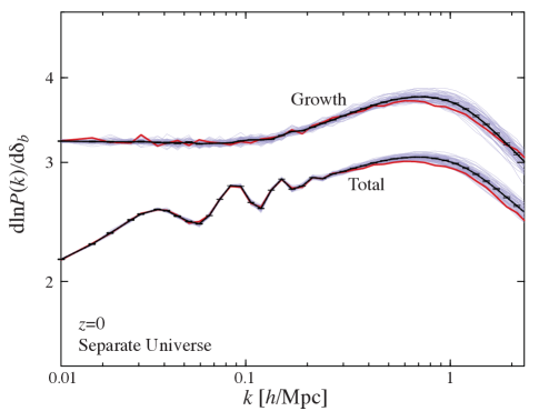
To compute the power spectrum response for a given cosmological model, we can use the separate universe approach developed in [Li et al. (2014)]. In this approach the impact of the super-box mode is absorbed into changes in the background cosmological parameters in a finite-volume simulation with periodic boundary condition:
| (13) |
Here is the linear growth rate and we have introduced the notations such as , where denotes the parameter in a separate universe (a finite volume region at the fixed ). Our convention is to set the scale factor of the separate universe to agree with the global one at high redshift: . Since the linear background density evolves with , so ; the relations about cosmological parameters hold independently of the redshift at which and are defined. Thus, even if the global universe has a flat geometry, , the separate universe with non-zero is realized as a non-zero curvature universe, . Because this is the curvature effect, time evolution of all the sub-box Fourier modes is affected by the super-box mode, due to the modified expansion history.
Fig. 1 shows the power spectrum response computed using the separate universe approach. There are two distinct contributions to the power spectrum response. First, the presence of super-survey mode modifies the growth of sub-volume modes via the mode coupling in nonlinear structure formation. If the survey region is embedded in a coherently overdense region, i.e. , the growth of sub-volume modes is enhanced. We call this effect “growth”. Second, the super-survey mode causes remapping of physical and comoving length scales. An overdense region expands less quickly than in the global universe. We call this effect “dilation” as it changes the comoving scale corresponding to features in the power spectrum. The figure shows that, in the total, these two effects partially cancel, leaving a characteristic scale-dependence in the response. We also note that, if we use the halo model to estimate the power spectrum response by directly computing the windowed trispectrum, , the analytical prediction gives about 10%-level agreement with the separate universe result over the range of shown in Fig. 1.
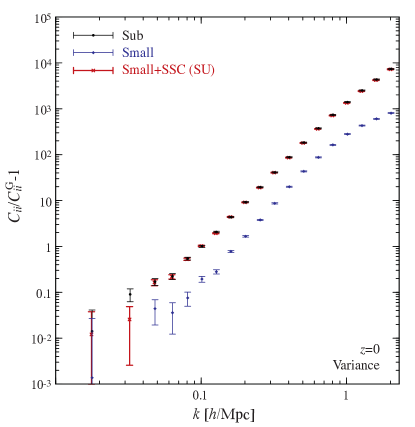
Upcoming wide-area galaxy surveys require an accurate estimation of the power spectrum covariance or more generally the covariance of any large-scale structure probes. This is indeed computationally challenging. With the unified theory of the covariance, Eq. (11), we can propose a way of calibrating the power spectrum covariance at computationally reasonable expense. To compute the standard part, the Gaussian piece and the trispectrum piece of sub-volume modes, we can use mock catalogs of a galaxy survey, based on N-body simulations of small boxes. To compute the SSC effect, we can use the separate universe simulations for the fiducial cosmology. In doing this, we can properly take into account the survey window to compute the linear variance, . This method does not require huge-volume simulations whose size is designed to be well larger than the size of survey volume in order to include the super-survey effects.
In Fig. 2, we indeed show that the above method combining the small-box simulations and the separate universe simulations well reproduces the covariance matrix from the large-volume simulations. The figure also shows that the SSC effect boosts the covariance amplitude by up to an order of magnitude over the range of wavenumbers we consider. Hence the SSC effect is the dominant source of the sample variance. This results hold for any size of survey volumes relevant for upcoming galaxy surveys (see Fig. 1 in Takada & Hu 2013).
If the power spectrum needs to be estimated with respect to the local average density within the finite-volume survey region, which is the case for the galaxy power spectrum (Takada et al. 2014), the power spectrum response is modified as
| (14) |
where is the power spectrum with respect to the local average density. The SSC effect is reduced in the covariance of the local power spectrum, but still gives a dominant contribution in the nonlinear regime (Li et al. 2014).
The small-scale, nonlinear version of the SSC effect can also be realized within the framework of the halo model approach – the halo sample variance (HSV) ([Hamiltonetal:06, Hu & Kravtsov 2003, Takada & Bridle (2007), Takada & Jain (2009), Sato et al. (2009), Kayo et al. (2013), Takada & Hu (2013), Takada & Spergel (2014), Schaan et al. (2014), Hu & Kravtsov 03; Takada & Bridle 2007; Takada & Jain 2009; Sato et al. 2009; Kayo et al. 2013; Takada & Hu 2013; Takada & Spergel 2014; Schaan et al 2014]). In the halo model formulation, the 1-halo term of the mass power spectrum, which describes correlations between dark matter in the same halo, is expressed as
| (15) |
where is the halo mass function in the mass range , is the cosmic mean mass density, and is the Fourier transform of the mass density profile of halos of mass . However, the above equation is correct only in an ensemble average sense. For a finite-volume survey, the coherent density fluctuation across the survey window, , would change the abundance of halos in the survey region along the peak-background splitting theory:
| (16) |
where the notation denotes the average over the realizations of different sub-survey modes at fixed , and is the halo bias. Thus, e.g., if the survey region is in a coherent over-density region, it enhances the number of halos on average.
By inserting Eqs. (15) and (16) into the covariance formula (Eq. 11) via the trispectrum consistency relation, we find that the change in the halo mass function via the super-survey modes causes co-variant scatters in the power spectrum estimation:
| (17) | |||||
where we have assumed that the super-survey modes do not affect the halo mass profile. We found that the HSV effect gives a dominant contribution of the SSC effect in the power spectrum covariance at a few , fairly well reproducing the separate universe simulation results at the scales ([Takada & Hu (2013), Li et al. (2014), see Fig. 2 Takada & Hu 2013 or Fig. 1 in Li et al. 2014]).
3.2 Information content of lensing power spectrum and bispectrum
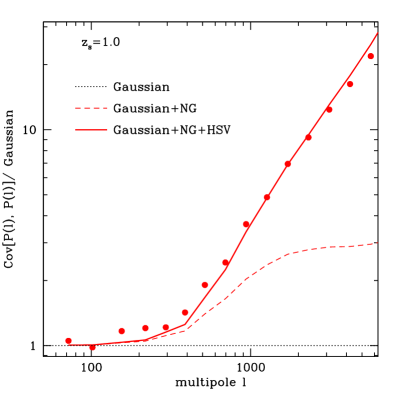
Similarly to the mass power spectrum covariance, we can compute the covariance matrices for the weak lensing power spectrum and bispectrum ([Takada & Bridle (2007), Takada & Jain (2009), Sato et al. (2009), Kayo et al. (2013), Takada & Spergel (2014), Schaan et al. (2014), Takada & Bridle 2007; Takada & Jain 2009; Sato et al. 2009; Kayo et al. 2013; Takada & Spergel 2014; Schaan et al. 2014]). The left panel of Fig. 3 shows diagonal elements of the weak lensing power spectrum covariance relative to the Gaussian covariance, measured from the ray-tracing simulations that are built using a suite of N-body simulations for the WMAP CDM model ([Sato et al. (2009), Sato et al. 2009]). We used 1000 realizations for source redshift each of which has an area of 25 sq. degrees corresponding to the fundamental Fourier mode . The ray-tracing simulations were done in a light cone volume with an observer’s position being its cone vertex, and therefore include contributions from N-body Fourier modes with length scales greater than the light-cone volume at each lens redshift (see Fig. 1 in Sato et al. 2009). Thus the simulations are suitable to study the SSC effect. As can be found from the figure, the weak lensing power spectrum covariance shows significant non-Gaussian errors at a few hundreds. The solid curve denotes the analytical prediction including the HSV effect, showing remarkably nice agreement with the ray-tracing simulation result. We note that the HSV effect causes highly correlated scatters between different multipoles. If we ignore the HSV effect, i.e. include the standard non-Gaussian error alone arising from the lensing trispectrum of sub-survey modes, the model prediction significantly underestimates the total power.
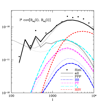
Similarly the right panel of Fig. 3 shows the results for the bispectrum covariance matrix. Here we consider the equilateral triangle configurations. The HSV effect gives a dominant contribution to the total power of the covariance matrix at , compared to other terms up to the 6-point correlation function. If we include the HSV contribution, the analytical model gives a 10-20% level agreement with the simulation results.
Once the covariance matrices for the weak lensing power spectrum and bispectrum are computed, we can address the information content carried by the weak lensing correlation functions. For a given range of multipoles, the cumulative signal-to-noise ratio or the information content for the power spectrum measurement is defined as
| (18) |
where the summation runs over all multipole bins in the range and is the inverse of the covariance matrix. The inverse of is equivalent to a precision of measuring the logarithmic amplitude of the power spectrum up to a given maximum multipole , assuming that the shape of the power spectrum is perfectly known. Similarly we can define the values for the bispectrum measurement and for a joint measurement of the power spectrum and the bispectrum. For the latter case, we need to properly take into account their cross-covariance.
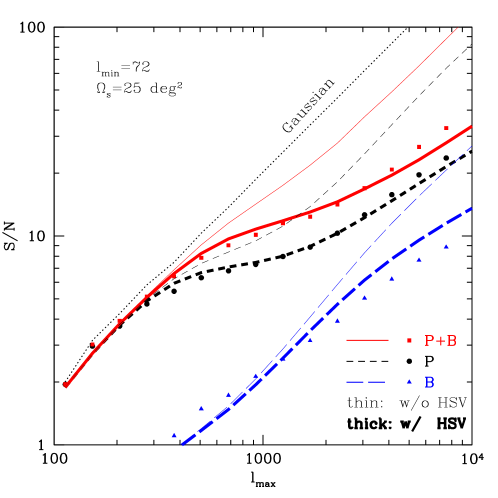
Fig. 4 shows the expected for measurements of the weak lensing power spectrum and bispectrum for a survey area of 25 square degrees (i.e. the area of the ray-tracing simulation), as a function of the maximum multipole up to which the power spectrum and/or bispectrum information are included. The minimum multipole is fixed to . Roughly speaking the value scales with survey area as (exactly speaking the scaling does not hold due to the different dependence of the SSC effect on survey area). The circle, triangle and square symbols are the simulation results for the power spectrum, the bispectrum and the joint measurement, respectively. For the bispectrum measurement we included the bispectra of all triangle configurations available from the multipole range, and considered up to 204 triangles for . The thick/thin short-dashed, long-dashed and solid curves are the analytical predictions with/without the HSV effects. First, the figure clearly shows that the lensing bispectra add new information content to the power spectrum measurement. To be more quantitative, adding the bispectrum measurement increases the by about 50 per cent for compared to the power spectrum measurement alone. This improvement is equivalent to about 2.3 larger survey area for the power spectrum measurement alone; that is, the same data sets can be used to obtain the additional information, if the bispectrum measurement is combined with the power spectrum measurement. Secondly, the analytical predictions are in nice agreement with the simulation results. Note that the total for the joint measurement is close to the linear sum of the values, not the sum of their squared values , due to the significant cross-covariance. If ignoring the cross-covariance, adding the bispectrum measurement does not much improve the (only by 5 per cent or so).
The top, dotted lines shows the information content for a Gaussian field, which the initial density field of large-scale structure should have contained – therefore can be considered as a maximum information content we could ultimately extract. The Gaussian information content depends only on the number of Fourier modes available from the range of multipoles up to : it has a simple scaling given by . The figure shows that the joint measurement can recover only about 50% or less of the Gaussian information at . The information loss is mainly due to the HSV effect, as can be found from the thin curves. If we ignore the HSV effect, the joint measurement recovers about 70% of the Gaussian information at . These results imply that further higher-order functions such as the 4-point function may be important and add the information ([Seo et al. (2011), see Seo et al. 2011]). Or some of the initial Gaussian information is lost or cannot be recovered due to the nonlinear clustering. This is not yet known, and still an open question.
3.3 Weak lensing tomography

Adding redshift information to the weak lensing correlation functions greatly improves the cosmological sensitivity – the so-called weak lensing tomography ([Takada & Jain (2004), Takada & Jain 2004]). However, to realize the genuine power of the weak lensing tomography, we need to consider all the spectra available from all possible combinations of different redshift bins and multipole bins. For the bispectrum case, adding the lensing tomography easily leads to more than 1000 bispectra, and this is even worse for the higher-order correlations. Hence, an accurate calibration of the covariance matrix for the lensing tomography would require a huge number of independent ray-tracing simulations, e.g., a factor 10 more realizations than the number of bispectra to achieve about 10% accuracy. This is computationally very challenging, and is even impossible if we need to compute the covariance as a function of cosmological models. So again a hybrid method combining small-box simulations, separate-universe simulations, and the analytical model would be useful and tractable in practice.
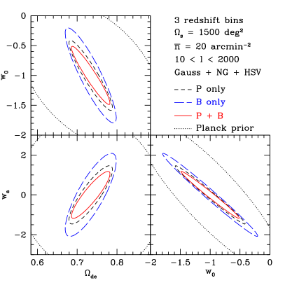
In Kayo & Takada (2013), we used the halo model approach, which gives a fairly good agreement with the simulation results for no tomography case as shown in Fig. 4, in order to estimate the cosmological power of the weak lensing bispectrum tomography. Fig. 5 shows expected accuracies of dark energy parameters assuming survey parameters that resemble the Subaru Hyper Suprime-Cam, characterized by sq. degrees, arcmin-2 and for the survey area, the mean number density of source galaxies and the rms intrinsic ellipticities per component, respectively. The bispectrum further adds the information to improve the parameter constraints compared to the power spectrum alone. To be more precise, for the three redshift bin case (the right panel), the joint measurement leads to about 60% improvement in the dark energy figure-of-merit (FoM) that is defined by . Again this is equivalent to about 60% larger survey area for the power spectrum tomography alone. In this case we considered 6525 triangle configurations, and we take into account the non-Gaussian correlations between the different spectra including the HSV effects.
4 Discussion
Can we recover the initial Gaussian field from observables of the present-day large-scale structure? This is an unresolved, open question. In this paper we discussed the example of the weak lensing field that is the line-of-sight projection of the three-dimensional mass density field in large-scale structure. We showed that the information content inherent in the power spectrum, which is the two-point correlation function in Fourier space, is smaller than the Gaussian information by more than a factor of 2 at . We showed that the bispectrum, which is the three-point correlation function, does add the information to the power spectrum, but the combined information does not fully recover the Gaussian information – still only 50% of the Gaussian information at . In order to derive this conclusion, we included all the two- and three-point level information in a sense that we included the bispectra of all available triangle configurations for a given range of multipoles as well as properly took into account the auto- and cross-covariances between the two- and three-point correlation functions. This implies that the higher-order correlation functions are further needed to recover the Gaussian information. Or our result implies a limitation of the information recovery; some of the initial memory is lost due to the strong mode coupling in the deeply nonlinear regime. Alternatively, the nonlinear mapping of the cosmological field, such as the log-normal mapping (Seo et al. 2012), might be a more practically useful way.
However, this conclusion is a bit misleading. Most of the information loss is caused mainly by the super-sample covariance. As we showed, the super-survey effects are parameterized mainly by the average density fluctuation in the survey volume, , on each realization basis. Hence, by treating as an additional parameter together with cosmological parameters, we may be able to calibrate most of the super-sample variance effects in the correlation measurements ([TakadaSpergel:13, Schaan et al. (2014), Li et al. (2014b), e.g., see Takada & Spergel 2013; Schaan et al. 2014; Li et al. in preparation]). We can even treat the super-survey mode as “signal” and then estimate its value for a given survey volume by fitting the measurements with the model. This is an interesting possibility, and needs to be further explored. A physical understanding of the super-survey effects is also important to explore an optimal survey design that allows an efficient operation of massive cosmological surveys (Takahashi et al. 2014).
Acknowledgments.– MT was supported by World Premier International Research Center Initiative (WPI Initiative), MEXT, Japan, by the FIRST program “Subaru Measurements of Images and Redshifts (SuMIRe)”, CSTP, Japan, and by Grant-in-Aid for Scientific Research from the JSPS Promotion of Science (Nos. 23340061 and 26610058).
References
- [Hamilton, Rimes & Scoccimarro 2006] Hamilton, A. J. S., Rimes, C. D., Scoccimarro, R. 2006, MNRAS, 371, 1188
- [Heymans et al. 2013] Heymans, C., et al. 2013, MNRAS, 432, 2433
- [Hu & Kravtsov 2003] Hu, W., & Kravtsov, A. 2003, ApJ, 584, 702
- [Kayo & Takada (2013)] Kayo, I., & Takada, M. 2013, arXiv:1306.4684
- [Kayo et al. (2013)] Kayo, I., Takada, M., Jain, B. 2013, MNRAS, 429, 344
- [Li et al. (2014)] Li, Y., Hu, W., Takada, M. 2014, Phys. Rev. D, 89, 083519
- [Li et al. (2014b)] Li, Y., Hu, W., Takada, M. 2014b, in preparation
- [More et al. (2014)] More, S., et al. 2014, arXiv:1407.1856
- [Oguri & Takada (2011)] Oguri, M., & Takada, M. 2011, Phys. Rev. D, 83, 023008
- [Sato et al. (2009)] Sato, M., Hamana, T., Takahashi, R., Takada, M., et al. 2009, ApJ, 701, 945
- [Seo et al. (2011)] Seo, H.-J., Sato, M., Dodelson, S., Jain, B., Takada, M. 2011, ApJ Letters, 729, 11
- [Schaan et al. (2014)] Schaan, E., Takada, M., Spergel, D. N. 2014, arXiv:1406.3330
- [Takada (2010)] Takada, M. 2010, AIP Conference Proceedings, 1279, 120
- [Takada & Bridle (2007)] Takada, M., & Bridle, S. 2007, New Journal of Physcis, 9, 446
- [Takada & Hu (2013)] Takada, M., & Hu, W. 2013, Phys. Rev. D, 87, 123504
- [Takada & Jain (2004)] Takada, M., & Jain, B. 2004, MNRAS, 348, 897
- [Takada & Jain (2009)] Takada, M., & Jain, B. 2009, MNRAS, 395, 2065
- [Takada & Spergel (2014)] Takada, M., & Spergel, D. N. 2014, MNRAS, 441, 2456
- [Takada et al. (2014)] Takada, M., Ellis, R. S., Chiba, M., Greene, J. E., et al. 2014, Publ. Astron. Soc. Japan, 66, R1
- [Takahashi et al. (2014)] Takahashi, R., Soma, S., Takada, M., Kayo, I. 2014, arXiv:1405.2666