The Sloan Lens ACS Survey. XII. Extending Strong Lensing to Lower Masses^†

Abstract

We present observational results from a new Hubble Space Telescope (HST) Snapshot program to extend the methods of the Sloan Lens ACS (SLACS) Survey to lower lens-galaxy masses. We discover 40 new galaxy-scale strong lenses, which we supplement with 58 previously discovered SLACS lenses. In addition, we determine the posterior PDFs of the Einstein radius for 33 galaxies (18 new and 15 from legacy SLACS data) based on single lensed images. We find a less-than-unity slope of $0.64\pm 0.06$ for the $\log_{10}{\sigma}_{*}$-$\log_{10}{\sigma}_{\rm SIE}$ relation, which corresponds to a 6-$\sigma$ evidence that the total mass-density profile of early-type galaxies varies systematically in the sense of being shallower at higher lens-galaxy velocity dispersions. The trend is only significant when single-image systems are considered, highlighting the importance of including both “lenses” and “non-lenses” for an unbiased treatment of the lens population when extending to lower mass ranges. By scaling simple stellar population models to the HST I-band data, we identify a strong trend of increasing dark-matter fraction at higher velocity dispersions, which can be alternatively interpreted as a trend in the stellar initial mass function (IMF) normalization. Consistent with previous findings and the suggestion of a non-universal IMF, we find that a Salpeter IMF is ruled out for galaxies with velocity dispersion less than $180$ km/s. Considered together, our mass-profile and dark-matter-fraction trends with increasing galaxy mass could both be explained by an increasing relative contribution on kiloparsec scales from a dark-matter halo with a spatial profile more extended than that of the stellar component.

1. Introduction

Early-type galaxies (ETGs), classified by their morphology, compose one of the two main categories of galaxies (Hubble, 1926, 1936). Although considered to be relatively “dead” and “featureless” as a consequence of their little star formation activities and smooth light distributions, ETGs play a crucial role in studying the evolution of galaxies, the nature of dark matter, and cosmology. Believed to be the endproducts of hierarchical merging scenario (Toomre & Toomre, 1972; White & Frenk, 1991; Kauffmann et al., 1993; Cole et al., 2000), their structures, properties, and formation histories can be used as a compelling test of the $\rm\Lambda$ Cold Dark Matter ($\rm\Lambda CDM$) paradigm. Additionally, ETGs can be extremely luminous and therefore can be used as powerful cosmological tracers of the large-scale structure (Eisenstein et al., 2005; Percival et al., 2007; Anderson et al., 2012).

However, the formation and evolution of ETGs are still puzzling and further investigations are highly demanded. Concerning the mass-density profile of ETGs, N-body DM-only numerical simulations have revealed a somewhat “universal” density profile with a $r^{-1}$ inner profile and a $r^{-3}$ drop-off at large radii, independent of the halo mass (Navarro et al., 1996, 1997). Later on, various observations of DM-dominated galaxies yield inconsistent inner density slopes with numerical simulations (Moore et al., 1999; Graham et al., 2006; Navarro et al., 2010), the tension of which can be loosened by taking baryonic physics into account. Gas cooling permits baryons to condense in the central regions of galaxies, and therefore it is believed to make the mass distribution more centrally concentrated (e.g. Gnedin et al., 2004; Gustafsson et al., 2006; Abadi et al., 2010; Velliscig et al., 2014). Heating due to dynamical friction and supernovae (SN)/Active Galactic Nucleus (AGN) feedback, in contrast, can soften the central density concentration (e.g. Nipoti et al., 2004; Romano-Díaz et al., 2008; Governato et al., 2010; Duffy et al., 2010; Martizzi et al., 2012; Dubois et al., 2013; Velliscig et al., 2014). The strength of these competing effects differs from galaxy to galaxy and hence studying the dependences of the shape of the mass-density profile in the central region on galaxy mass, redshift, and other structural quantities unravels the formation and evolution of ETGs.

The stellar initial mass function (IMF) is an empirical relation quantifying the relative fraction of stars as a function of the stellar mass at the time when the whole population formed. Salpeter (1955) first quantified the IMF as a simple power-law function using main-sequence stars in the solar neighborhood. Later on, various modifications have been considered at the low-mass end and the most commonly used forms are the Kroupa IMF (Kroupa, 2001) and the Chabrier IMF (Chabrier, 2003). The IMF of a galaxy could depend on the environmental properties of the molecular cloud it originated from such as metallicity, temperature, and density, and could therefore be non-universal. Having knowledge of the form and the variation of the IMF provides deep insights in understanding the role of the environment during star formation and galaxy evolution processes. Recently, several pieces of evidence suggest that the IMF indeed varies (e.g. Treu et al., 2010; Auger et al., 2010b; van Dokkum & Conroy, 2010; Strader et al., 2011; Cappellari et al., 2012; Sonnenfeld et al., 2012; Spiniello et al., 2012; Ferreras et al., 2013; La Barbera et al., 2013; Conroy et al., 2013; Tortora et al., 2013; Brewer et al., 2014; Spiniello et al., 2014).

Strong gravitational lensing (GL) has its unique power among the many techniques for the study of ETGs. As a pure gravity-dependent effect, GL provides highly accurate measurements of total mass that are robust against different models and assumptions about galaxy properties. Therefore, it provides the best estimation of the total projected mass within the so-called Einstein radius enclosed by the lensed images of the background object.

One of the known issues in estimating the enclosed mass by GL is the mass-sheet degeneracy (MSD), in which a proper mass-density transformation preserves the dimensionless lensing observables such as image positions, shapes, flux ratios, etc. (e.g, Falco et al., 1985; Gorenstein et al., 1988; Narayan & Bartelmann, 1996; Schneider & Sluse, 2013). Given lensing data alone, breaking this degeneracy requires some additional physical assumptions. However, following Treu et al. (2009), a qualitative estimations of the effect of MSD on our final results are presented in Section 4. Further information including stellar kinematics can fully break the MSD degeneracy.

Various lensing surveys have been conducted in the past decade and led to numerous important results. The Lenses Structure and Dynamics (LSD) Survey aimed to measure the stellar kinematics of a small sample of E/S0 galaxy lenses and combine it with GL to constrain the central mass distribution (Koopmans & Treu, 2002, 2003; Treu & Koopmans, 2002, 2004). The SLACS survey (Bolton et al., 2006; Treu et al., 2006; Koopmans et al., 2006; Gavazzi et al., 2007; Bolton et al., 2008a; Gavazzi et al., 2008; Bolton et al., 2008b; Treu et al., 2009; Auger et al., 2009, 2010a; Newton et al., 2011) is by far the most productive survey for galaxy-scale strong lenses with known lens and source redshifts, with a discovery of over 90 spectroscopically-selected lenses confirmed by high-resolution Hubble Space Telescope (HST) follow-up. SLACS observes relatively low-redshift ($z_{L}\lesssim 0.4$) ETG lens candidates selected from the Luminous Red Galaxy (LRG, Eisenstein et al., 2001) and MAIN (Strauss et al., 2002) galaxy samples of the Sloan Digital Sky Survey (SDSS, York et al., 2000). The SLACS survey has yielded multiple novel results on the structure and dynamics of ETGs, which are detailed in the previous papers of this series. Recently, the technique of spectroscopic lens selection has been extended to earlier cosmic time (higher redshift) by the BOSS Emission-Line Lens Survey (BELLS, Brownstein et al., 2012), which has confirmed 25 strong lenses ($0.4\lesssim z_{L}\lesssim 0.7$) using data from the Baryon Oscillation Spectroscopic Survey (Dawson et al., 2013) of the SDSS-III (Eisenstein et al., 2011).

The SLACS sample is a unique resource for studies of the structure of ETGs. As studied by Arneson et al. (2012), no significant bias in the mass axis ratio relative to the parent population is detected in spectroscopically selected lens samples (See also Sonnenfeld et al. (2014)). And the selection bias in the mass-density profile slope is rather small, estimated by Bolton et al. (2012b) to be on the order of $\sim 0.01$ for a combined sample of SLACS and BELLS lenses. However, it is known that the SLACS selection function favors the high-mass end due to several related factors. First, strong lensing cross section (an approximation of the lensing possibility in general) increases with the lens galaxy mass, so high-mass ETGs are more likely to act as strong lenses. Second, even if a low-mass galaxy acts as a strong lens, the characteristic angular separation of the lensed images will be small and hard to resolve even at space-based imaging resolution. Third, low-mass galaxies can be intrinsically too faint to be selected for SDSS spectroscopy. Fourth, for the preceding reasons, high-mass SLACS candidates have been prioritized for HST follow-up during previous SLACS programs, in order to maximize the survey success rate.

In order to extend the power of strong lensing to low-mass galaxies, an extension of the SLACS survey known as “SLACS for the Masses” (hereafter S4TM, HST Snapshot Program 12210) was initiated in April 2012 with a focus on lens candidates with lower masses and smaller predicted Einstein radii as compared to SLACS lenses. While the lensing confirmation rate of S4TM is lower than that of previous SLACS HST programs, it importantly achieves a wider lens-mass baseline in combination with previous SLACS lenses. Note that the Sloan WFC Edge-on Late- type Lens Survey (SWELLS, Treu et al., 2011) also probes low-mass lenses albeit with a focus on spiral galaxies. We refer the readers to the S4TM catalog paper by Brownstein et al. 2015 (in preparation) for a full description of the S4TM program details. In this paper, we present the first scientific results on the total mass-density profile and dark-matter content of an extended ETG sample combining the S4TM lenses and previous SLACS lenses. We use a hierarchical Bayesian method to infer the mass-profile scaling relation of the combined lens sample, and estimate stellar masses through single stellar-population (SSP) model scalings to the observed HST photometry.

This paper is organized as follows. In Section 2, we briefly describe our lens identification technique using the SDSS spectroscopy and high-resolution imaging data observed by the HST. Section 3 describes our parametric lens-modeling method. We then derive the main findings in Sections 4 and 5 with regards to the study of the mass-density profile and dark-matter fraction of the ETGs. Discussion and conclusions are presented in Section 6. Throughout the paper, we assume a standard cosmology with $\rm\Omega_{m}=0.274$, $\rm\Omega_{\Lambda}=0.726$ and $\rm H_{0}=70\,km\,s^{-1}\,Mpc^{-1}$ (WMAP7, Komatsu et al., 2011).

2. Lens Candidate Identification

The S4TM survey is a snapshot program designed to extend strong gravitational lensing observations toward lower masses and relatively smaller Einstein radii as compared to previous SLACS programs. Using the same lens searching technique as SLACS, 137 lens candidates were identified from the seventh data release (DR7) of the SDSS (Abazajian et al., 2009) and awarded as HST snapshot targets in Observing Cycle 18. The details about the lens selection technique can be found in the papers by Bolton et al. (2006, 2008a) and Brownstein et al. 2015 (in preparation). The basic approach is to search for high-redshift emission lines such as [Oii] doublets, H$\beta$, and [Oiii] superimposed on the spectra of SDSS target galaxies at lower redshifts. Such emission lines, associated with star-forming galaxies more distant along the same line of sight, indicate the presence of a candidate lensing system, and also allow us to simultaneously determine the redshifts of the background objects.

Between 2010 September and 2012 June, 118 out of 137 candidates were successfully observed with an exposure time of 420 s each with a single exposure through the F814W filter of the Wide Field Channel (WFC) of the Advanced Camera for Surveys (ACS). The images were visually inspected using the ACSPROC software, a GUI tool implemented by Brownstein et al. (2012). By searching for lensed features in the b-spline-subtracted residual images (Bolton et al., 2006, 2008a), we have confirmed 40 strong gravitational lenses with clear and definite multiple lensed images or even complete Einstein rings (classified as “grade-A”), 8 systems with strong evidence of multiple imaging but insufficient SNR for definite conclusion and/or modeling (classified as “grade-B”), as well as 18 systems showing clear images of the background objects but no clear counter-images (classified as “grade-C”). We exclude one grade-C lens ($\rm SDSSJ1310+0220$) from now on as it turned out to be a face-on late-type galaxy with strong emission lines after an examination of its SDSS spectrum.

3. Lens Modeling and Sample Definition

For the foreground lens galaxies, we consider a singular isothermal ellipsoid (SIE) lens model (Kassiola & Kovner, 1993; Kormann et al., 1994; Keeton & Kochanek, 1998; Bolton et al., 2008a) that is generalized from a singular isothermal sphere (SIS) model in which the 2D surface mass density falls off as $R^{-1}$, but consists of elliptical iso-density contours specified by position angle $P.A.$ and minor-to-major axis ratio $q_{\rm SIE}$. We do not include external shear in our lens model as it has been shown by Koopmans et al. (2006), Treu et al. (2009), and confirmed again using our grade-A lens sample to be a minor effect. Discussions on the effect of external shear on the final results are presented in Section 4.3. The SIE lens model is characterized by the lensing strength $b_{\rm SIE}$ (specified according to an “intermediate axis” convention for elliptical models).

$$b_{\rm SIE}=4\pi\frac{\sigma_{\rm SIE}^{2}}{c^{2}}\frac{d_{LS}}{d_{S}},$$ (1)

where $d_{LS}$ and $d_{S}$ are the angular diameter distances from the lens and the observer to the source, respectively.

The relationship between the $b_{\rm SIE}$ Einstein-radius parameter and the “lens-model velocity dispersion” $\sigma_{\rm SIE}$ given in Equation 1 is, strictly speaking, only valid for the case of circular symmetry. For the elliptical case, we take Equation 1 to be our implicit definition of $\sigma_{\rm SIE}$. By this convention, $b_{\rm SIE}$ is the intermediate axis (geometric mean of semi-major and semi-minor axes) of the isodenisty contour within which the average convergence $\kappa$ is equal to unity. As discussed by Huterer et al. (2005), an alternative convention is to adopt the radius of a circle (denoted $\theta_{\rm E}$ in that work) within which the average $\kappa$ is unity. We adopt the $b_{\rm SIE}$ convention in this work to enable us to use the empirical relation of Auger et al. (2010a) (which adopts the same convention) between mass-density profile and the ratio of stellar to lensing velocity dispersions. We explore the sensitivity of our results to this choice in Section 4.3 using the ellipicity-dependent $b_{\rm SIE}$-$\theta_{\rm E}$ relation from Huterer et al. (2005), which is accurate to $<1\%$ on average within the axis-ratio ranges of our lenses.

The surface brightness distribution of sources are represented by either one or multiple Sérsic components with the form

$$I(x,y)\propto{\rm exp}[-\frac{1}{2}(\frac{qx^{2}+y^{2}/q}{\sigma^{2}})^{n/2}],$$ (2)

with the axis ratio $q$, width $\sigma$, and exponent $n$ as free parameters.

For a particular SIE lens model and specific composition of the source, one can generate the predicted lensed images via the ray-tracing technique according to the analytical expressions of the lens equation (Kormann et al., 1994). We apply different fitting strategies to grade-A and grade-C lenses as explained in the following subsections. Note that for all the lens imaging data, we rescale the corresponding errors such that the average error of the background matches the standard deviation of the background to correct for possible correlations in the errors caused by image resampling.

3.1. Lens Modeling: Grade-A Lenses

Figure 1.— A comparison of the derived Einstein radii between this work and the published SLACS values for 58 grade-A lenses confirmed by the SLACS survey. The ratios are consistent with 1 with a $\rm rms=0.005$ which suggests that our code is robust.

For each of the 40 newly discovered grade-A lenses in the S4TM survey, the fitting strategy is relatively straightforward. A Levenberg-Marquardt non-linear least-squares fit (MPFIT, Moré, 1978; Markwardt, 2009) to the observed lensed images is performed to obtain the best-fit parameters for both the lens and the source. Distinct multiple lensed images/rings ensure accurate and unambiguous model fits. We use the position angle $P.A._{*}$ and axis ratio $q_{*}$ extracted from the b-spline fit to the light distribution as initial guesses. The starting value for $b_{\rm SIE}$ is determined from the separation between a lensed image and its counter-image. Depending on the configuration of the lensing features, one or multiple source components are considered to ensure a reasonably good fit.

We also apply the same fitting strategy to 58 grade-A lenses found in the SLACS survey, and show the results in Figure 1. It is clear that the derived Einstein radii of this work are consistent with the published values in Bolton et al. (2008a) with an average scatter of $0.5\%$. In subsequent analyses, we adopt this scatter as the fractional uncertainty in the measured Einstein radii for grade-A lenses since the statistical errors significantly underestimate the uncertainties as discussed by Bolton et al. (2008a).

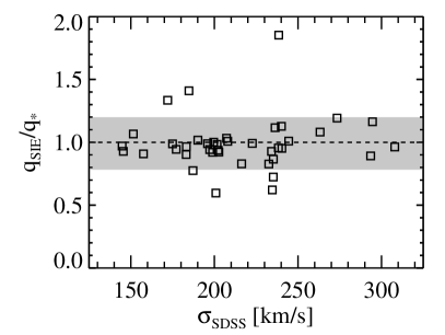
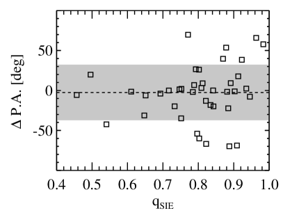
Figures 2 and 3 compare the axis ratios and position angles of the light distribution to those of the mass distribution for the grade-A subsample. Figure 2 displays the ratios of the minor-to-major axis ratio as a function of the SDSS stellar velocity dispersion $\sigma_{\rm SDSS}$ which is consistent with $1.0$ with a rms scatter of $0.2$. No correlation with the velocity dispersion (an approximation of the total mass) is observed. Figure 3 visualizes the difference in the position angle $\Delta P.A.=P.A.-P.A._{*}$ of lenses with respect to the axis ratios. $\langle\Delta P.A.\rangle=-2^{\circ}$ with a rms spread of $34^{\circ}$. Clearly, as either $q_{\rm SIE}$ or $q_{*}$ goes to $1$, the position angle becomes ill-determined and the scatter increases significantly. Note that $|\Delta P.A.|$ are smaller than $31^{\circ}$ for all but one S4TM grade-A lens with both $q_{*}$ and $q_{\rm SIE}$ less than $0.8$. Therefore, in general, the hypothesis of light tracing mass is valid in terms of both the match of isophotal and isodensity contours and the position-angle alignment and indicates little external perturbing potential. In general, our SIE lens models with multiple parameterized sources can successfully recover the overall lensing features as well as small details.

Figure 2.— Ratio between the minor-to-major axis ratio determined from SIE model fitting $q_{\rm SIE}$ and that measured from light distribution $q_{*}$ as a function of velocity dispersion for 40 S4TM grade-A lenses. The shaded gray region indicates the rms spread (see text for details).

Figure 3.— Discrepancy in the position angle determined from SIE model fitting $P.A.$ and that measured from light distribution $P.A._{*}$ as a function of $q_{\rm SIE}$ for 40 S4TM grade-A lenses. The shaded gray region indicates the rms spread (see text for details).

3.2. Lens Modeling: Grade-C Lenses

In comparison with “grade-A” lenses, the systems we refer to as “grade-C lenses” (i.e., without counter-images) are less informative about the mass structure of the foreground galaxy (in addition to being less visually striking). However, while these grade-C lenses do not provide accurate lens mass measurements, they do provide accurate lens-mass probability distributions. Furthermore, as will be seen later, grade-C systems are relatively less massive, and hence, the lens-mass probability distributions that they provide are an essential element of our program to extend strong-lensing science to lower lens masses. Indeed, the inclusion of such single-image systems to a lens ensemble analysis makes the selection function less sharply dependent on lens galaxy mass as compared to the grade-A lens sample alone.

Nevertheless, in most previous gravitational lensing studies, grade-C lens systems have been ignored because of the difficulty or impossibility of obtaining definite lens mass models. (A significant counterexample is the use of lensing ”flexion” to constrain mass models in systems that allow this technique: Goldberg & Leonard (2007).) This difficulty is particularly pronounced within pure imaging surveys for lenses, because background galaxies with no clear multiple imaging can easily be confused with satellite galaxies of the foreground lens. For the case of the S4TM program, however, we have a strong prior for the identification of singly imaged background galaxies due to the original spectroscopic detection of a second redshift along the line of sight.

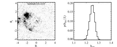
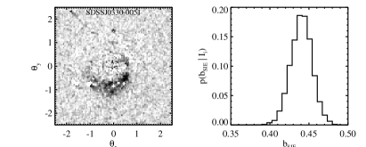
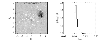
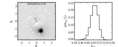
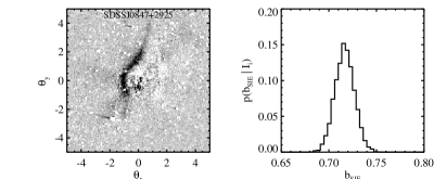
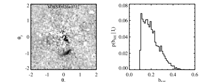
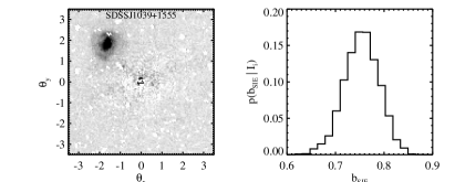
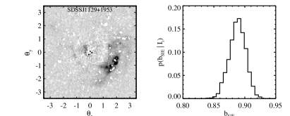
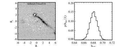
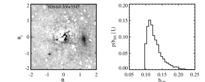
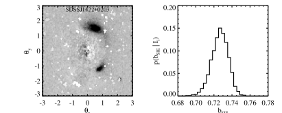
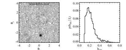
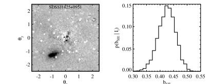
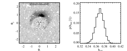
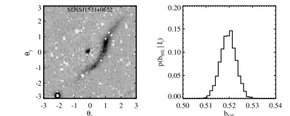
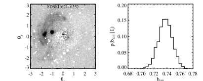
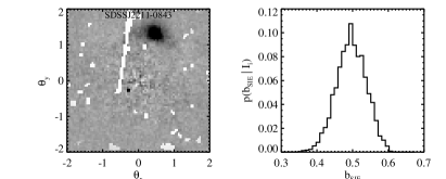
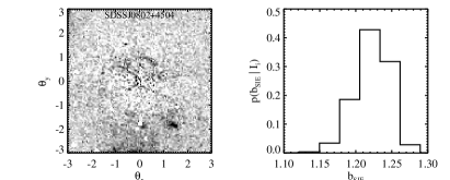
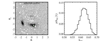
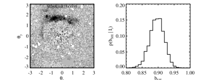
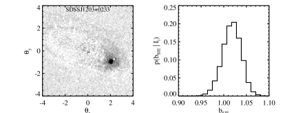
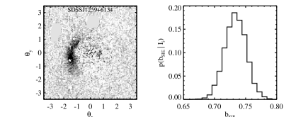
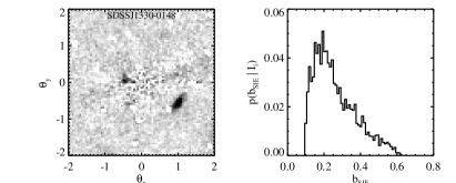
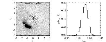
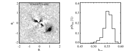
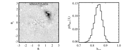
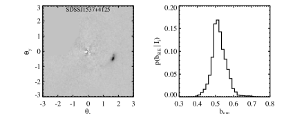
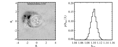
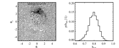
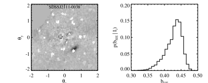
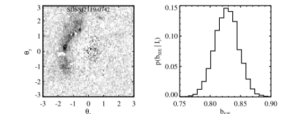
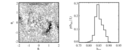
In this work, we explicitly incorporate grade-C lenses into our analysis, by first determining their posterior probability density functions (PDFs) of the Einstein-radius, and subsequently incorporating these PDFs into our ensemble analysis of the scaling relations of the lens population via a hierarchical Bayesian method. In order to obtain the posterior PDFs of $b_{\rm SIE}$, we utilize the MultiNest package (Feroz & Hobson, 2008; Feroz et al., 2009, 2013; Buchner et al., 2014) which is a Bayesian inference tool designed to efficiently compute the evidence of models in high dimensions through nested sampling. For highly complex multimodal distributions with pronounced degeneracies, such as the grade-C lens modelings in our case, it has been demonstrated that MultiNest significantly outperforms traditional Markov Chain Monte Carlo (MCMC) techniques. We assume uniform priors with appropriate bounds for all the lens and source parameters. In particular, we require the total mass profiles of grade-C lenses to be not flatter than the light distributions by explicitly setting $q_{\rm SIE}\geq q_{*}$. This special requirement stems from the fact that the fitting code can converge to unphysical lens models with very small axis ratios and small lensing strength for grade-C systems. As shown previously by Koopmans et al. (2006); Bolton et al. (2008b); Barnabè et al. (2011) and confirmed again by the grade-A subsample in the S4TM survey (Figure LABEL:fig:light_mass), the hypothesis of a mass quadrupole following the light quadrupole is generally valid, and the requirement of mass being not flatter than light is well-motivated. Figures  11 and 12 in the Appendix Section show the foreground-subtracted images and posterior PDFs of $b_{\rm SIE}$ for S4TM and SLACS grade-C lenses, respectively.

3.3. Combined Sample

We also run MultiNest on grade-A lenses and find their posterior PDFs of $b_{\rm SIE}$ can be well described by extremely narrow Gaussian functions with means consistent with the best-fit $b_{\rm SIE}$ values from MPFIT. Therefore we approximate the posterior PDFs of $b_{\rm SIE}$ for grade-A lenses as delta functions. We then combine both posterior PDFs to perform unbiased analyses of the mass structure of ETGs across a wider range of galaxy masses. In the following sections, we combine these measurements with stellar velocity dispersions and broadband photometry to constrain the mass-density profile and dark-matter fraction of ETGs as a function of galaxy mass.

Figure 4.— Distributions of the stellar mass $M_{*}^{\rm Chab}$ for the whole grade-A+C sample (black), SLACS grade-A subsample (blue), S4TM grade-A subsample (green), SLACS grade-C subsample (chocolate), and S4TM grade-C subsample (red) and the median values for each subsample. The stellar mass is derived from the HST I-band photometry by the SPS analysis assuming a Chabrier IMF and other parameters (please refer to Section 5 for details).

Figure 5.— Distribution of the predicted Einstein radii $b_{\rm SIE}$ and the stellar mass $M_{*}^{\rm Chab}$ for all the modeled lenses. Open squares represents grade-A lenses, with 40 from the S4TM survey (green) and 58 from the SLACS survey (blue). We do not show uncertainties for grade-A lenses as they have been quantified to be on the level of $0.5\%$ (Figure 1) which are much smaller than the symbol size. Grade-C lenses are filled circles with error bars indicating the 1$\sigma$ uncertainties inferred from the posterior PDFs.

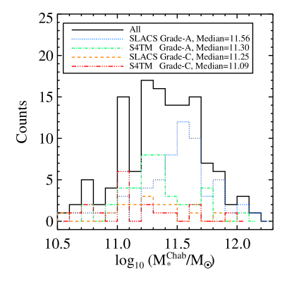
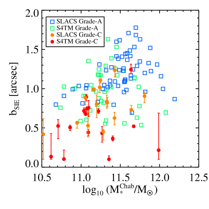
Combining the S4TM survey and the SLACS survey generates a data set including 98 (40+58) grade-A and 33 (18+15) grade-C ETG lens systems. The mean redshift for the foreground lenses is $\langle z_{L}\rangle=0.18$ and $\langle z_{S}\rangle=0.58$ for the background sources. The distributions and median values of the stellar masses (derived from the HST F814W photometry assuming a Chabrier IMF and the fiducial stellar-population model of Section 5 below) for various subsamples are also plotted in Figure 4. Note that the S4TM lenses are generally less massive compared to the SLACS lenses and grade-C lenses are generally less massive than grade-A lenses. Figure 5 shows the distribution of the Einstein radius $b_{\rm SIE}$ and stellar mass for all the 131 lenses. For grade-A lenses, only the measurements of $b_{\rm SIE}$ are plotted as the uncertainties have been shown to be on the level of $0.5\%$ which are much smaller than the symbol size. For grade-C lenses, the most likely $b_{\rm SIE}$ values and the 1$\sigma$ uncertainties inferred from the posterior PDFs of $b_{\rm SIE}$ are displayed.

4. Mass Structure Analysis

In this section, we combine the posterior PDFs of $b_{\rm SIE}$ for both grade-A and grade-C lenses with lens-galaxy stellar velocity dispersions measured from SDSS spectroscopy in order to constrain the mass-density profile of ETG lenses as a function of lens-galaxy mass. The inclusion of new S4TM systems and grade-C lenses allows us to explore a broader range of galaxy masses than previous studies.

4.1. Velocity-Dispersion Proxy

To investigate the degree of central concentration of ETG mass profiles, we employ an observational proxy defined by the ratio of stellar velocity dispersion to the SIE model velocity dispersion $\sigma_{\rm SIE}$, defined in relation to the observable parameter $b_{\rm SIE}$ through Equation (1). It was suggested by Kochanek (1994) that this ratio, later denoted as $f_{\rm SIE}=\sigma_{*}/\sigma_{\rm SIE}$, should be approximately unity for isothermal mass models, greater than unity for models more centrally concentrated than isothermal, and less than unity for models less centrally concentrated. Successive studies have confirmed this hypothesis and showed that $f_{\rm SIE}$ can be used as an empirical indicator of the mass-density slope (Kochanek et al., 2000; Treu & Koopmans, 2002, 2004; Treu et al., 2006; Koopmans et al., 2006; Bolton et al., 2008b; Treu et al., 2009; Auger et al., 2010a). We take this approach in the current work in order to investigate physical trends and their significance in the simplest possible manner, and defer a more detailed and self-consistent joint analysis of gravitational lensing and stellar kinematics to future papers.

As mentioned above, the posterior PDFs of $\sigma_{\rm SIE}$ are converted directly from the posterior PDFs of $b_{\rm SIE}$. The other ingredient for our present analysis is the stellar velocity dispersion $\sigma_{*}$, which is the standard deviation of velocities of stars within a galaxy. This quantity is determined spectroscopically by measuring the broadening of the galaxy spectrum due to the luminosity-weighted superposition of Doppler-shifted absorption lines from individual stars. Instead of adopting the preexisting SDSS stellar velocity-dispersion values calculated using a set of stellar spectra templates derived from ELODIE stellar spectrum library (Prugniel & Soubiran, 2001) with wavelength coverage 4100Å-6800Å, we generate a new set of stellar templates from the Indo-US library (Valdes et al., 2004) patched and extended by selected synthetic spectra in POLLUX database (Palacios et al., 2010), covering the full wavelength range of observed spectra. More details about this procedure can be found in Bolton et al. (2012a, b). The resulting velocity dispersions $\sigma_{\rm SDSS}$ are then corrected to values within one half of the half-light radius $\rm R_{half}/2$ (a quantity that is comparable to the lens-galaxy Einstein radius as shown in Bolton et al. (2008a) and confirmed again by our lens sample) following a compromise prescription between Jorgensen et al. (1995); Mehlert et al. (2003) and Cappellari et al. (2006) as

$$\sigma_{*}=\sigma_{\rm SDSS}\times(\frac{1.5^{\prime\prime}}{\rm R_{half}/2})^{0.05},$$ (3)

where $1.5^{\prime\prime}$ is the angular radius of the SDSS fiber. The half-light radius $R_{\rm half}$ is derived from a core-Sérsic fit (Graham et al., 2003) to the surface brightness distribution of each lens galaxy as explained in Brownstein et al. 2014 (in preparation).

4.2. Hierarchical Bayesian Analysis

Our primary interest here is in the physical scaling relation between $\sigma_{*}$ and $\sigma_{\rm SIE}$ that encodes the variation of the mass-density profile within the ETG lens population. In the formalism of statistics, we treat this as a conditional probability density function (PDF) of $\sigma_{*}$ given $\sigma_{\rm SIE}$.

We parameterize the mean scaling relation between $\log_{10}{\sigma}_{*}$ and $\log_{10}{\sigma}_{\rm SIE}$ as

$$(\log_{10}{\sigma}_{*}-2.35)=a\times(\log_{10}{\sigma}_{\rm SIE}-2.35)+b,$$ (4)

with a slope $a$ and intercept $b$. The constant shift of $2.35$ is introduced to reduce the correlation between $a$ and $b$. And the value itself is chosen to match the average value of $\log_{10}{\sigma}_{*}$. To constrain the parameters of this relation, we use the hierarchical Bayesian method (see e.g., Shu et al., 2012; Bolton et al., 2012b; Brewer et al., 2013; Sonnenfeld et al., 2013; Sonnenfeld et al., 2014). This method makes full use of all the observed information, deconvolves the observational uncertainties, and offers unbiased estimations of population “hyperparameters” that we are interested in. The hierarchical Bayesian approach also allows for straightforward inclusion of the posterior PDFs of $b_{\rm SIE}$ in the analysis.

Table 1Key ingredients for the hierarchical Bayesian analysis.

Symbol	Definition
$x$	Parameter 1: $\log_{10}\sigma_{\rm SIE}$
$y$	Parameter 2: $\log_{10}\sigma_{*}$
$I_{i}$	Data 1: HST imaging data for lens $i$
$y_{i}$	Data 2: measured value of $\log_{10}\sigma_{*}$ for lens $i$
$a$	Hyperpar. 1: slope of $\log_{10}{\sigma}_{*}$-$\log_{10}{\sigma}_{\rm SIE}$
$b$	Hyperpar. 2: intercept of $\log_{10}{\sigma}_{*}$-$\log_{10}{\sigma}_{\rm SIE}$
$\delta$	Hyperpar. 3: intrinsic scatter in $\log_{10}\sigma_{*}$
$\vec{\theta}$	Vector of hyperparameters
$\mathrm{Pr}(y_{i}|y)$	Likelihood function of $y$ given $y_{i}$
$\mathrm{Pr}(y,x|\vec{\theta},\mathscr{H})$	Joint PDF of parameters given $\vec{\theta}$
$\mathrm{Pr}(y|x,a,b,\delta,\mathscr{H})$	PDF of parameter $y$ given $x$, $a$, $b$, and $\delta$
$\mathrm{Pr}(b_{\rm SIE}|I_{i},q,\phi)$	Posterior PDF of $b_{\rm SIE}$ given $I_{i}$, $q$, and $\phi$

Here we describe all the key ingredients in the hierarchical Bayesian analysis. $x$, $y$ represent the two physical parameters $\log_{10}\sigma_{\rm SIE}$, $\log_{10}\sigma_{*}$, and $I_{i}$, $y_{i}$ are the corresponding observed data for the $i^{th}$ lens galaxy. The three hyperparameters (compacted as $\vec{\theta}$) we want to determine are i) $a$: the slope of $\log_{10}{\sigma}_{*}$-$\log_{10}{\sigma}_{\rm SIE}$ relation; ii) $b$: the intercept; iii) $\delta$: the intrinsic scatter in $\log_{10}{\sigma}_{*}$.

Following the same strategy used by Shu et al. (2012), the likelihood function of hyperparameters $\vec{\theta}$ given the observed data $\{\vec{d}\}$ and a hypothesis $\mathscr{H}$ is defined as

$$\mathscr{L}(\vec{\theta}|\{\vec{d}\} ,\mathscr{H})\equiv\mathrm{Pr}(\{\vec{d}\}|\vec{\theta},\mathscr{H})=\prod_{i=0}^{N}\,\mathrm{Pr}(y_{i},I_{i}|\vec{\theta},\mathscr{H})$$

$$=\prod_{i=0}^{N}\iint\mathrm{Pr}(y_{i},I_{i}|y,x)\mathrm{Pr}(y,x|\vec{\theta},\mathscr{H})\mathrm{d}x\mathrm{d}y.$$

In general, $y$ and $x$ are independent variables and $\mathrm{Pr}(y_{i},x_{i}|y,x)$ can be split as

$$\mathscr{L}(\vec{\theta}|\{\vec{d}\},\mathscr{H}) =\prod_{i=0}^{N}\iint\mathrm{Pr}(y_{i}|y)\mathrm{Pr}(I_{i}|x)\mathrm{Pr}(y,x|\vec{\theta},\mathscr{H})\mathrm{d}x\mathrm{d}y$$

$$=\prod_{i=0}^{N}\iint\mathrm{Pr}(y_{i}|y)\mathrm{Pr}(y|x,a,b,\delta,\mathscr{H})\mathrm{Pr}(I_{i}|x)$$

$$\hskip 47.23167pt\mathrm{Pr}(x)\mathrm{d}x\mathrm{d}y.$$ (5)

The last two terms of the above equation is related to the posterior PDF of $b_{\rm SIE}$ as

$$\mathrm{Pr}(I_{i}|x)\mathrm{Pr}(x)\mathrm{d}x=\mathrm{Pr}(b_{\rm SIE}|I_{i})\mathrm{Pr}(b_{\rm SIE})\mathrm{d}b_{\rm SIE}.$$ (6)

Then the likelihood function becomes

$$\mathscr{L}(\vec{\theta}|\{\vec{d}\},\mathscr{H})=\prod_{i=0}^{N}\iiiint\mathrm{d}y\mathrm{d}q\mathrm{d}{\phi}\mathrm{d}b_{\rm SIE}\,\mathrm{Pr}(y_{i}|y)$$

$$\mathrm{Pr}(y|x,a,b,\delta,\mathscr{H})\mathrm{Pr}(b_{\rm SIE}|I_{i},q,\phi)\mathrm{Pr}_{i}(q)\mathrm{Pr}_{i}(\phi).$$ (7)

Looking at each term, $\mathrm{Pr}(y|y_{i})$ is the likelihood function of $y$ given $y_{i}$, which can be written as

$$\mathrm{Pr}(y_{i}|y)=\frac{1}{\sqrt{2\pi}\delta_{i}}\mathrm{exp}[-\frac{(y-y_{i})^{2}}{2\delta_{i}^{2}}].$$ (8)

$\mathrm{Pr}(y|x,a,b,\delta,\mathscr{H})$ is the conditional PDF of $y$ given $x$ and three hyperparameters. Following the parameterized model stated by Equation (4), $\mathrm{Pr}(y|x,a,b,\delta,\mathscr{H})$ can be expressed as

$$\mathrm{Pr}(y|x,a,b,\delta,\mathscr{H})=$$

$$\,\,\,\frac{1}{\sqrt{2\pi}\delta}\mathrm{exp}\{-\frac{[a(x-2.35)+b-(y-2.35)]^{2}}{2\delta^{2}}\},$$ (9)

with an assumed intrinsic scatter $\delta$ in $y$. $\mathrm{Pr}(y|x,a,b,\delta,\mathscr{H})$ is of physical interest as it quantifies the relation between $y$ and $x$ and can be adopted in related studies. $\mathrm{Pr}(b_{\rm SIE}|I_{i},q,\phi)$ is the posterior PDF of $b_{\rm SIE}$ as returned by MultiNest given the imaging data $I_{i}$, axis ratio $q$, and position angle $\phi$. $\mathrm{Pr}_{i}(q)$ and $\mathrm{Pr}_{i}(\phi)$ are the prior PDFs of $q$ and $\phi$ for the $i^{th}$ lens galaxy, which are assumed to be uniform distributions.

The integration over $y$ can be easily done and yields

$$\mathscr{L}=\prod_{i=0}^{N}\,\iiint\mathrm{d}q\mathrm{d}{\phi}\mathrm{d}b_{\rm SIE}\, \frac{\exp[-(\Delta-y_{i})^{2}/(2(\sigma_{i}^{2}+\delta^{2}))]}{\sqrt{2\pi(\sigma_{i}^{2}+\delta^{2})}}$$

$$\mathrm{Pr}(b_{\rm SIE}|I_{i},q,\phi)\mathrm{Pr}_{i}(q)\mathrm{Pr}_{i}({\phi}),$$ (10)

where $\Delta=a\times[x(b_{\rm SIE})-2.35]+b+2.35$.

For grade-A lenses, we can treat $\mathrm{Pr}(b_{\rm SIE}|I_{i},q,\phi)$, $\mathrm{Pr}_{i}(q)$, and $\mathrm{Pr}_{i}({\phi})$ as delta functions. The likelihood contribution from grade-A lenses is

$$\ln\mathscr{L}_{A}=-\sum_{i=0}^{N_{A}}\{\frac{(\Delta(b_{\rm SIE}^{i})-y_{i})^{2}}{2(\sigma_{i}^{2}+\delta^{2})}+0.5\times\ln[2\pi(\sigma_{i}^{2}+\delta^{2})]\}.$$ (11)

For the $i^{th}$ grade-C lens, MultiNest generates samples of $b_{\rm SIE}^{ij}$ with derived posteriors (or weights) $\mathrm{Pr}(b_{\rm SIE}^{ij}|I_{i},q,\phi)$. The likelihood contribution is therefore approximated as

$$\ln\mathscr{L}_{C}=\sum_{i=0}^{N_{C}}\ln\{\sum_{j=0}^{N} \frac{\exp[-(\Delta(b_{\rm SIE}^{ij})-y_{i})^{2}/(2(\sigma_{i}^{2}+\delta^{2}))]}{\sqrt{2\pi(\sigma_{i}^{2}+\delta^{2})}}\times$$

$$\mathrm{Pr}(b_{\rm SIE}^{ij}|I_{i},q,\phi)\}.$$ (12)

The posterior PDF of the hyperparameters that we are interested in is simply related to the likelihood via the Bayes’ rule as

$$\mathrm{Pr}(\vec{\theta}|\{\vec{d}\},\mathscr{H}) = \frac{\mathrm{Pr}(\{\vec{d}\}|\vec{\theta},\mathscr{H})\,\mathrm{Pr}(\vec{\theta}|\mathscr{H})}{\mathrm{Pr}(\{\vec{d}\}|\mathscr{H})}$$

$$= \frac{\mathscr{L}(\vec{\theta}|\{\vec{d}\},\mathscr{H})\,\mathrm{Pr}(\vec{\theta}|\mathscr{H})}{\mathrm{Pr}(\{\vec{d}\}|\mathscr{H})},$$ (13)

from which we can infer the relation between $\log_{10}\sigma_{*}$ and $\log_{10}\sigma_{\rm SIE}$.

Known as $f_{\rm SIE}$, the ratio of $\sigma_{*}$ to $\sigma_{\rm SIE}$ has been used as an empirical estimator of the logarithmic mass-density slope $\gamma^{\prime}$ (Treu et al., 2009; Auger et al., 2010a). Using the $\sigma_{*}$-$\sigma_{\rm SIE}$ relation found above, by definition, we have

$$f_{\rm SIE}=\frac{\sigma_{*}}{\sigma_{\rm SIE}}=10^{y-x} =10^{[({a}-1)(y-2.35)+{b}]/{a}}$$

$$=10^{(a-1)(x-2.35)+b}.$$ (14)

The physical interpretation of hyperparameters $a$ and $b$ then become straightforward. If $a$ is exactly unity, $f_{\rm SIE}$ (or equivalently the logarithmic mass-density slope $\gamma^{\prime}$) is independent of $\sigma_{*}$, an indicator of the mass of lens galaxies. A less-than-unity $a$ indicates an anti-correlation between $\gamma^{\prime}$ and $\sigma_{*}$, namely galaxies with smaller/larger $\sigma_{*}$ are more/less centrally concentrated. $b$ is related to the $f_{\rm SIE}$ value at the mean $\sigma_{\rm SIE}$ value ($\sigma_{\rm SIE}\approx 220$ km/s). The mass-density profile is (approximately speaking) isothermal if $b=0$, sub-isothermal if $b<0$, and super-isothermal if $b>0$.

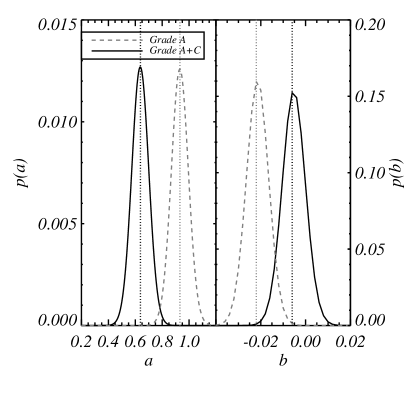
Marginalizing over the $\delta$ dimension, the 2D posterior PDF of $a$ and $b$ is shown in Figure 6. There are three sets of contours for grade-A subsample (dashed gray), grade-C subsample (dotted gray), and the combined sample (solid black). The marginal PDFs of $a$ and $b$ are obtained by marginalizing over either $b$ or $a$ and shown in Figure 7. The best-estimated values for $a$ and $b$ and the uncertainties are extracted from simple Gaussian fits to the corresponding marginal PDFs, and summarized in Table 2.

Figure 6.— The posterior PDFs of $(a,b)$ for the combined sample (solid black contours), grade-A subsample (dashed gray contours), and grade-C subsample (dotted gray contours). $68\%$, $95\%$, and $99.7\%$ confidence levels are plotted accordingly. The horizontal line ($b=-0.0338$ as suggested by the empirical relation in Auger et al. (2010a)) corresponds to an isothermal mass-density profile at $\sigma_{\rm SIE}\approx 220$ km/s, and the vertical line ($a=1$) corresponds to a velocity-dispersion-independent mass-density profile.

Figure 7.— The marginal PDFs of $a$ and $b$ for the combined sample (grade-A+C lenses, solid black curves) and grade-A lens subsample (dashed gray curves). Dotted lines corresponds to the peak positions in the marginal PDFs.

Table 2The best-estimated values of the two hyperparameters $a$ and $b$ derived from the corresponding marginal PDFs for grade-A subsample (2nd row) and grade-A+C sample (3rd row). By including grade-C lenses, the slopes become significant shallower.

Lens Sample	$a_{\rm best}$	$b_{\rm best}$
Grade A	$0.93\pm 0.06$	$-0.021\pm 0.005$
Grade A+C	$0.64\pm 0.06$	$-0.005\pm 0.005$

We see that for the grade-A lens subsample, the overall mass-density profile is essentially consistent with a mass-independent model at about 1.1$\sigma$ ($P(a<1.0)=85.49\%$), as found in previous SLACS studies (e.g., Bolton et al., 2008b; Auger et al., 2010a). Grade-C lenses alone can not provide meaningful constraints on the hyperparameters given such broad posterior PDF distribution. However, the combination of grade-A and grade-C systems in the analysis significantly shifts the grade-A results and provides evidence for a mass-dependent density profile at about 6$\sigma$. The sense of this trend is for lower mass (i.e., lower velocity-dispersion) ETGs to have steeper mass-density profiles and higher mass ETGs to have shallower profiles.

Note that our current results for grade-A systems are consistent with previous SLACS results of a velocity-dispersion-independent density profile. Similarly, the parameters from our current analysis of grade-A+C systems are substantially consistent with the results of our current grade-A-only analysis. Hence our detection of a velocity-dispersion-dependent density profile in this work is fundamentally due to the inclusion of new data for new lenses covering a wider baseline in mass, and is not an artifact of the new methods we have applied in the analysis of these data.

Consulting the empirical relation between the mass-density profile slope $\gamma^{\prime}$ and the observable $f_{\rm SIE}$ from Auger et al. (2010a), we find that a value of $b=-0.0338$ corresponds on average to an isothermal profile ($\gamma^{\prime}=2$). Considering the best-fit value for $b$ for the grade-A subsample, we find that it is somewhat inconsistent with isothermal at about 2.3$\sigma$. Including grade-C systems as well, the best $b$ value is more strongly inconsistent with isothermal at $>5\sigma$. In both cases, the offset is in the sense of having a slightly super-isothermal profile at the central lensing velocity-dispersion of the samples, consistent with previous SLACS findings (Koopmans et al., 2009).

4.3. Systematic Effects on Mass Structure

As previously mentioned, several issues in the lens modeling procedure have not been fully addressed yet, including the environmental contributions, discrepancy between $b_{\rm SIE}$ and $\theta_{\rm E}$, and the intrinsic nonisothermality of the lens galaxies. In this section, we investigate the individual effects of the above issues on our mass-structure results.

4.3.1 Environmental effects

Figure 8.— Fractional discrepancy of the Einstein radius (top panel) and ratio of axis ratio (bottom panel) as a function of the “true” axis ratio when fitting mock images generated from an SIE+external shear model by an SIE model (please refer to the text for details).

Here we discuss the environmental effects on our mass-structure estimation caused by neglecting possible extra contributions from the environment, i.e., MSD and external shear. Following the recipe in Treu et al. (2009), we write the “true” total convergence as

$$\kappa(x,y)=\frac{\sqrt{q}}{2}\frac{R_{\rm SIE}^{0}}{\sqrt{x^{2}+q^{2}y^{2}}}+\kappa_{\rm ext},$$ (15)

where the first term on the right-hand-side is the contribution from the SIE lens, and the second term is used to quantify the contribution from external convergence (i.e. mass sheet). $R_{\rm SIE}^{0}$ is the “true” Einstein radius for the lens galaxy assuming an SIE model.

The total projected mass within an ellipse of axis ratio $q$ and semi-minor axis $R^{\prime}$ is

$$M_{\rm total} =\Sigma_{\rm crit}\iint\kappa(x,y)\mathrm{d}x\mathrm{d}y$$

$$=\pi\Sigma_{\rm crit}({R_{\rm SIE}^{0}R^{\prime}}+{{R^{\prime}}^{2}}\kappa_{\rm ext}),$$ (16)

where $R^{\prime}=R/\sqrt{q}$ (geometric mean of the semi-major and semi-minor axises), and $\Sigma_{\rm crit}$ is the critical density. Note that here, for first-order approximation, an uniform external convergence $\kappa_{\rm ext}$ is assumed. In the “intermediate axis” convention we have been working with, the Einstein radius $R_{\rm SIE}$ we would infer by neglecting the external convergence is given by

$$R_{\rm SIE}^{2}=\frac{M_{\rm total}}{\pi\Sigma_{\rm crit}}=R_{\rm SIE}^{0}R_{\rm SIE}+R_{\rm SIE}^{2}\kappa_{\rm ext}.$$ (17)

Therefore, the “true” Einstein radius $R_{\rm SIE}^{0}$ differs from the value inferred from our SIE model $R_{\rm SIE}$ by a factor of $(1-\kappa_{\rm ext})$

$$R_{\rm SIE}^{0}=R_{\rm SIE}(1-\kappa_{\rm ext}).$$ (18)

From the scaling law between total projected mass and radius, Treu et al. (2009) estimated the external convergence $\kappa_{\rm ext}$ for SLACS lenses is no more than a few percent, and no significant bias was detected. Therefore we expect the effect of neglecting external convergence in our analysis is subdominant to measurement errors. Also as suggested by Bolton et al. (2012b), the external convergences are fluctuations about the mean densities, and only introduce random noise rather than bias, which will be smoothed out within our analysis.

The external shear $\gamma$ that we choose to dismiss turns out to be also a minor effect. In order to quantify it, we fit an SIE+external shear model with fixed axis ratio and position angle to the S4TM grade-A lenses and compare the resulted Einstein radii to values obtained by an SIE model. The overall fractional discrepancy is on the level of $2\%$, which suggest that the effect is again subdominant. To explore any degeneracy between external shear and axis ratio, we generate a set of mock lensed images from an SIE+external shear model with uniformly distributed axis ratios for the SIE profile. The lens galaxy and source are placed at typical lens and source redshifts, respectively. Typical noise level is also added to the mock images. The amplitude of the external shear is set to the mean shear found by Holder & Schechter (2003) at $0.11$ (also consistent with results in Wong et al. (2011)), and the position angle of the external shear is marginalized over. We then fit the mock images using an SIE model, and compare the so-obtained Einstein radii to the fiducial value. The results are shown in Figure 8. It is clear that we are able to recover the Einstein radii within an accuracy of about $4\%$ for the entire axis-ratio range. More importantly, we do not observe any significant correlation between the discrepancy in the Einstein radius and the axis ratio.

4.3.2 $b_{\rm SIE}$ convention VS. $\theta_{\rm E}$ convention

As previously mentioned, the $b_{\rm SIE}$ convention for an elliptical case is generally not identical to the $\theta_{\rm E}$ convention for a circular case. The conversion between $b_{\rm SIE}$ and $\theta_{\rm E}$ has been derived in Huterer et al. (2005) as a function of ellipticity (or axis ratio $q$ in our model). By definition, the deviation from $\theta_{\rm E}$ converges to 0 as $q$ approaches 1. Here we use all the 98 grade-A lenses to explore the sensitivity of our final results to the different conventions.

We first convert $b_{\rm SIE}$ obtained by the SIE modeling to $\theta_{\rm E}$ following Huterer et al. (2005), and then incorporate $\sigma_{\rm SIE}$ predicted by $\theta_{\rm E}$ into the Bayesian analysis. Given the facts that the mean axis ratio of the grade-A sample is $0.789$ and there is no significant correlation between $\sigma_{*}$ and $q$, converting $b_{\rm SIE}$ to $\theta_{\rm E}$ will only introduce an almost constant offset of $-0.002$ on average in $\log_{10}\sigma_{\rm SIE}$, which consequently gets propagated into an offset in $b$, but leaves the slope $a$ untouched. This expectation has been verified as we find that the posterior PDF of $a$ and $b$ is almost identical except for a tiny positive shift ($\sim 0.001$) in the marginal PDF of $b$.

We think the grade-A subsample is representative of the entire sample in terms of the axis-ratio distribution. Therefore, we conclude that the choice of different conventions in the analysis is only a minor effect on the final mass structure results.

4.3.3 Intrinsic nonisothermality

It has been suggested in this paper that the intrinsic mass profile is a varying function of galaxy mass, being steeper than isothermal in lower-mass galaxies. This deviation from isothermality confirms recent findings by Sonnenfeld et al. (2013); Dutton & Treu (2014), and Sonnenfeld et al. (2014). The effect of neglecting the intrinsic nonisothermality in the SIE modeling needs to be investigated. In order to do that, we fit 40 S4TM grade-A lenses by a singular power-law ellipsoid (SPLE) model for 5 discrete logarithmic mass-density slopes $\gamma^{\prime}$ from $1.5$ to $2.5$, and compare the so-obtained lensing strength $b_{\rm SPLE}$, which we think is a better approximation for the lensing velocity dispersion, to $b_{\rm SIE}$. We find that the majority of them suggests a correlation between the deviation from the “true” value defined as $b_{\rm SIE}-b_{\rm SPLE}$ and logarithmic slope $\gamma^{\prime}$. Following the mass-structure trend observed in this paper, it indicates that we tend to overestimate $\sigma_{\rm SIE}$ in low-mass galaxies ($\gamma^{\prime}>2$) and underestimate $\sigma_{\rm SIE}$ in high-mass galaxies ($\gamma^{\prime}<2$). That would in turn yield an even more pronounced mass-structure trend than we have seen. We defer further quantitative studies to future papers. Nevertheless, we confirm that neglecting the intrinsic nonisothermality can not alleviate the detected mass dependence of the total mass-density profile in the central region.

5. Stellar Masses and Initial Mass Function

In addition to allowing measurements of the shape of the lens mass-density profile, strong lensing data can be combined with photometry and stellar-population diagnostics to constrain the dark-matter fraction and/or stellar IMF in the lens (e.g. Treu et al., 2010; Ferreras et al., 2010; Spiniello et al., 2011; Grillo & Christensen, 2011; Spiniello et al., 2012; Sonnenfeld et al., 2012; Brewer et al., 2014). For this purpose, we estimate stellar masses of lens galaxies based on scaling of SSP models to HST I-band photometry under a range of stellar-population assumptions, and adopting either a Chabrier or Salpeter IMF. This simplicity is motivated by uniformity, since although multi-band HST photometry is available for many of the SLACS lenses, all the new S4TM systems currently have I-band data alone. High-resolution HST imaging is essential to masking the contribution from lensed background sources when performing lens-galaxy photometric modeling (Brownstein et al. 2014 in preparation). For this reason, we disregard multi-band SDSS photometric magnitudes in our analysis.

Figure 9.— Stellar masses $M_{*}$ of the 130 lenses inferred from the SPS analysis for the two IMFs as a function of the stellar velocity dispersion. Filled symbols are for the S4TM lenses and open symbols for the SLACS lenses. Grade-C lenses are shown by stars and grade-A lenses are circles. Colors represent the redshifts of the lens galaxies. Gray error bars represent the systematic variations (see text for details on how to determine the error bars). The correlation of scatter with redshift is primarily driven by Malmquist bias in the parent samples.

Figure 10.— Relations between the dark-matter fraction $f_{\rm dm}$ and $\log_{10}M_{*}^{\rm Chabrier}$, $\log_{10}\sigma_{*}$, and $\log_{10}\rm R_{half}$, respectively. Filled symbols represent S4TM lenses while open symbols are for SLACS lenses. Grade-C lenses are shown by stars and grade-A lenses are circles. Colors represent the redshifts of the lens galaxies. Gray error bars represent the systematic variations. Either a Chabrier or Salpeter IMF is considered.

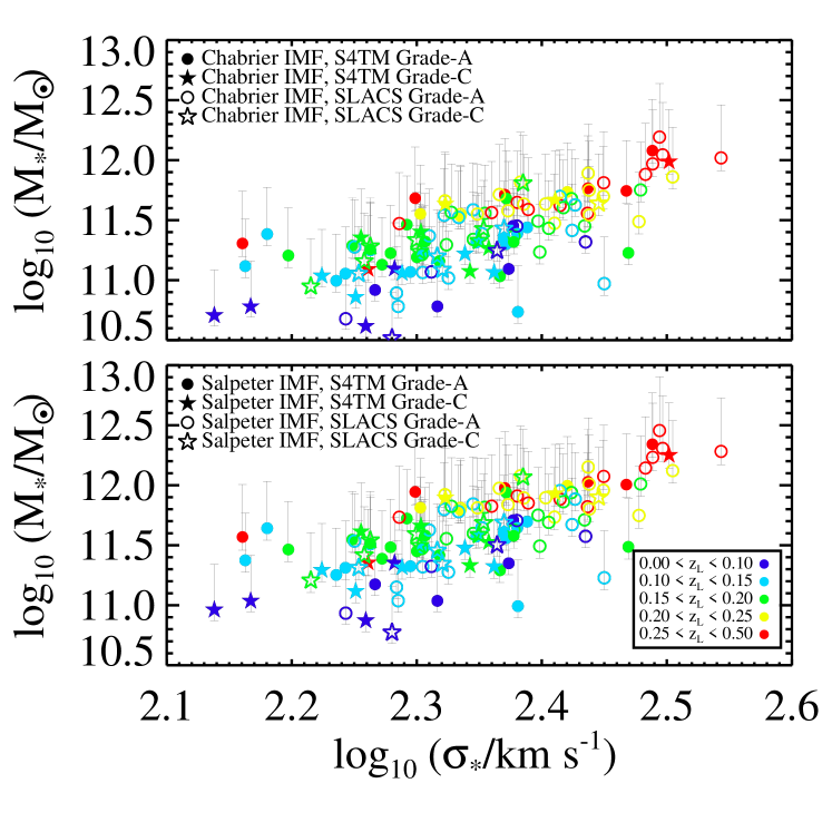
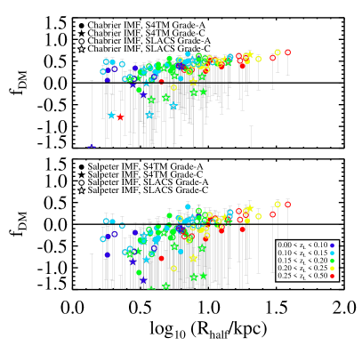
To translate photometry into stellar masses, we make use of SSP models obtained with the Flexible Stellar Population Synthesis (FSPS: Conroy et al., 2009; Conroy & Gunn, 2010). Without colors or narrow-band indices, we must necessarily make assumptions about population parameters such as the formation time after the Big Bang $t_{\rm form}$, metallicity, and dust in the FSPS code. Since all the lens galaxies are by selection ETGs at relatively low redshifts, we adopt a reference model with typical values of $t_{\rm form}=4$ Gyrs, solar metallicity, and no dust (Gallazzi et al., 2006; Carson & Nichol, 2010). We cross-check our stellar mass estimations with the values obtained by Auger et al. (2009) from multi-band HST photometric data and a Bayesian stellar population analysis approach for 52 confirmed SLACS lenses in common and find good agreement with no bias observed. To quantify the systematic uncertainty of the simple treatment, we also consider lower- and upper-bound models. Our lower-bound model is dust-free and metal-poor ($\log_{10}Z/Z_{\sun}=-0.30$), while our upper-bound model is dusty and metal-rich (the optical depth for the dust attenuation $\tau=0.95$, $\log_{10}Z/Z_{\sun}=0.20$). The level of the resulting systematic variation in estimated stellar mass is around 0.5 dex. Figure 9 shows the stellar masses of the 130 lenses from both the S4TM survey (filled symbols) and the SLACS survey (open symbols) for the reference model as a function of the stellar velocity dispersion. In accordance with the well-known Faber-Jackson relation (FJR, Faber & Jackson, 1976), galaxies with higher velocity dispersions also have higher stellar masses on average.

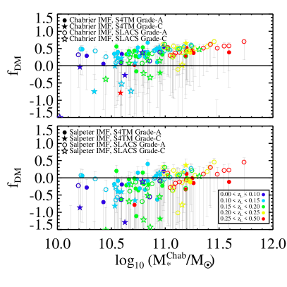
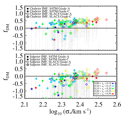
We next examine the relationships between the projected dark-matter fraction within one half of the half-light radius $f_{\rm dm}$ defined as $f_{\rm dm}\equiv 1-M_{*}(<\rm R_{half}/2)/M_{\rm R_{half}/2}$ and the stellar mass, the stellar velocity dispersion, and the half-light radius, respectively. The half-light radius $\rm R_{half}$ is determined by the core-Sérsic fit as the radius within which the enclosed light is one half of the total profile light. The stellar mass within one half of the half-light radius $M_{*}(<\rm R_{half}/2)$ is interpolated according to the underlying core-Sérsic profile under the assumption of a constant stellar-mass-to-light ratio for each galaxy. In Figure 10, symbols correspond to predictions by the model of $t_{\rm form}=4$ Gyrs, solar metallicity and dust-free for the two IMFs, respectively. In particular, stars represent grade-C lenses, and circles represent grade-A lenses. Filled symbols are S4TM lenses, while open symbols are SLACS lenses. The colors encode the redshifts of lens galaxies. Gray error bars show the systematic variations in $f_{\rm dm}$ throughout the parameter space as explained above. From Figure 10, we see general trends toward higher projected dark-matter fractions in galaxies with higher masses, larger velocity dispersions, and bigger sizes, consistent with detections by Auger et al. (2010a) using confirmed SLACS lenses. In all cases, the intrinsic scatter in $f_{\rm dm}$ is appreciable. More specifically, Panel (a) shows a strong correlation between $f_{\rm dm}$ and the stellar mass $M_{*}^{\rm Chabrier}(<\rm R_{half}/2)$ for either IMF, which we will thoroughly discuss in Section 6.1. The same behaviour can also be seen between Panels (b), which displays the relations between $f_{\rm dm}$ and the stellar velocity dispersion $\sigma_{*}$. Panel (c) suggests that bigger lens galaxies (larger $R_{\rm half}$ values) have larger matter-to-luminousity ratios in their central regions. These can be explained by the idea that the surface density of dark matter varies less slowly (as compared to the luminous matter) as the galaxy becomes more massive. It is also in line with previously detected correlations between $\gamma^{\prime}$ and stellar mass density (Sonnenfeld et al., 2013; Dutton & Treu, 2014). Of particular note, by implying a negative dark-matter fraction, the data strongly disfavor a Salpeter IMF for large fraction of the lenses, especially for those with stellar velocity dispersions $\sigma_{*}$ smaller than approximately $180$ km/s. This confirms a similar finding from Brewer et al. (2012) based on a much smaller number of spiral lens galaxies.

We have several avenues to improve the stellar-mass estimation. First of all, the significant scatter and systematic variation in $f_{\rm dm}$ and the IMF that we haven’t taken into account here will weaken any observed trends. A proper way to handle them is heavily required. On the lensing side, a simple SIE model for the total mass distribution as considered in this work, although is a good approximation, is not able to distinguish the contributions from dark and baryonic matter. Further physical assumptions need to be made to break the mass-density-profile-IMF degeneracy (Treu et al., 2010; Oguri et al., 2013). On the SPS side, age, metallicity, dust and other parameters in the SPS models need to be better constrained. Also it has been studied that the SPS technique highly relies on several IMF-sensitive spectral features such as NaI, CaII, FeH, TiO, and CaH1 (Conroy & van Dokkum, 2012; Spiniello et al., 2014). Improper interpretations in the SPS model, or lack of coverage of these features in the observed spectra can lead to significant systematics in constraining the IMF (Conroy & van Dokkum, 2012; Spiniello et al., 2014).

6. Discussion and Conclusion

In this paper, we report the discovery of 40 strong gravitational lenses with clear and definite multiple images (classified as “grade-A”) and another 18 single-image lenses (classified as “grade-C”) from the S4TM survey (HST Program ID 12210 , Brownstein et al.  2014 (in preparation)), which by design selects lens galaxies with lower masses and smaller Einstein radii compared to the previous SLACS survey. Along with findings in the SLACS survey, we construct a statistically significant and more complete ensemble of over 100 gravitational lenses, including 98 grade-As and 33 grade-Cs. This combined sample probes ETGs with a mean lens redshift of $\langle z_{L}\rangle=0.18$. All lenses have been modeled individually and measurements/posterior PDFs of the Einstein radii have been obtained for grade-A/C lens galaxies appropriately.

6.1. Discussion

We have discovered clear evidence for the dependence of the total mass-density profile on galaxy velocity dispersion, in the sense that less massive (lower velocity-dispersion) lens galaxies have more centrally concentrated (super-isothermal) profiles. We have obtained this result by performing a hierarchical Bayesian analysis of the relation between $\log_{10}\sigma_{*}$ and $\log_{10}\sigma_{\rm SIE}$ for the combined lens ensemble. The inclusion of grade-C lenses is essential to this discovery: the significance of the trend is about 6-$\sigma$ when including grade-A and grade-C lenses together in the analysis, but only about 1-$\sigma$ (i.e., consistent with no trend) when analyzing grade-A lenses alone. This can be attributed both to the fact that the grade-C lenses extend the mass baseline of the measurement to lower masses, and to the fact that excluding grade-C lenses will bias the sample towards higher values of $\sigma_{\rm SIE}$ at fixed $\sigma_{*}$. Note that this trend is in consistent with the overall trend seen going to even higher masses. In fact, in galaxy clusters, the slope is far from isothermal and closer to $\gamma^{\prime}=1$ (Newman et al., 2013a, b).

A trend of mass-density profile $\gamma^{\prime}$ upon the surface stellar mass density $\Sigma_{*}=M_{*}/(2\pi R_{\rm eff}^{2})$ has been found in Auger et al. (2010a), Sonnenfeld et al. (2013), and Dutton & Treu (2014) using either SLACS lenses or lenses from the Strong Lensing Legacy Survey (SL2S, Gavazzi et al., 2012; Gavazzi et al., 2014). In particular, they found that galaxies with denser stellar mass densities have steeper profiles. Since the stellar velocity dispersion can be approximated as $\sigma_{*}^{2}\propto M_{*}/R_{\rm eff}\propto\Sigma_{*}R_{\rm eff}$, the $\gamma^{\prime}$-$\sigma_{*}$ relation and $\gamma^{\prime}$-$\Sigma_{*}$ relation suggest that more massive galaxies are spatially less concentrated and have higher velocity dispersion at the present time. This can be understood in terms of the expectations from baryonic physics within DM halos. Dissipative gas cooling processes lead to higher baryon densities in the center of DM halos, and also steepen the DM halo profile through the effect of adiabatic contraction (AC: e.g., Blumenthal et al. 1986). Energetic feedback processes from SN and AGN tend to heat gas and counteract central condensation. These processes compete against each other in their effect on the mass distribution in DM halos. More importantly, the efficiencies of both cooling and feedback processes depend on galaxy mass/velocity dispersion. Our findings suggest that for less massive galaxies, the impact of feedback is less significant as compared to AC/cooling and hence leads to a more centrally concentrated halo. The importance of feedback increases as galaxies become more massive, resulting in shallower density profiles. Metallicity, environment and other processes are also responsible for this competition. In order to determine whether the effect is regulated primarily by velocity dispersion or by stellar density, multi-band data sufficient for detailed stellar-population analysis will be required for the full S4TM sample.

We have applied a simplified SPS analysis to the HST I-band photometric data to estimate the stellar masses of the lens galaxies assuming either a Chabrier or a Salpeter IMF. Age, metallicity and dust have been chosen to match the typical values for passively evolving ETGs at low redshifts. A clear correlation between the projected dark matter fraction and the total mass is observed for both IMFs, consistent with previous findings (e.g. Tortora et al., 2009; Auger et al., 2010a; Cappellari et al., 2012; Conroy et al., 2013; Brewer et al., 2014). There are two possible interpretations of this result: as a true increase in dark-matter fraction with velocity dispersion, or as a trend in the stellar IMF with velocity dispersion. The first interpretation aligns with the overall expectation of decreased star-formation efficiency with increasing halo mass for halos above $\sim 10^{8}$ $M_{\odot}$(e.g. Behroozi et al., 2010). This interpretation could also explain our observed trend in dark-matter profile slope: for a fixed stellar profile shape, an increased fractional mass contribution from a more spatially extended DM halo will result in a shallower total-mass density profile. Alternatively, a trend towards a more bottom-heavy IMF in more massive galaxies can cause the apparent effect of an increased DM fraction when a single IMF is assumed across all masses (e.g., Treu et al., 2010; van Dokkum & Conroy, 2010; Strader et al., 2011; Sonnenfeld et al., 2012; Spiniello et al., 2012; Ferreras et al., 2013; La Barbera et al., 2013; Geha et al., 2013; Conroy et al., 2013; Tortora et al., 2013; Spiniello et al., 2014). Given the limited data set used in this paper, we are not able to distinguish between the two interpretations. Additional assumptions or data are necessary to break this degeneracy (e.g., Sonnenfeld et al., 2012; Sonnenfeld et al., 2014). However, the Salpeter IMF is in any event disfavored at the low-mass end, since it results in unphysical negative DM fractions.

6.2. Conclusion and Future Work

To conclude, in this paper,

1. We report the discovery of 40 new grade-A and 33 new grade-C ETG lenses from the S4TM and SLACS surveys. Besides the measurements for grade-A lenses, posterior PDFs of the Einstein radii for grade-C lenses are determined for the first time using the MultiNest tool. Combining with 58 grade-A ETG lenses from the SLACS survey, we construct an ETG lens ensemble with wider mass coverage than previous strong-lens samples;

2. Applying a hierarchical Bayesian method which utilizes the posterior PDFs of the Einstein radii, we study the correlation between $\log_{10}{\sigma}_{*}$ and $\log_{10}{\sigma}_{\rm SIE}$, and find a less-than-unity slope of $0.64\pm 0.06$ which corresponds to a significant ($\approx$6$\sigma$) dependence of total mass-density profile on the lens mass in the sense that more massive ETGs possess shallower profiles (as quantified by the ratio of $\sigma_{*}$ to $\sigma_{\rm SIE}$ which serves as a proxy for the logarithmic mass-density profile slope $\gamma^{\prime}$). We have shown that this trend is only significant when grade-C lenses are included (the slope is $0.93\pm 0.06$ for the grade-A only subsample), which highlights the importance of grade-C lenses to enabling a wider coverage of lens masses;

3. Stellar masses of lens galaxies are estimated based on their HST I-band photometry and SPS models assuming either a Chabrier or Salpeter IMF. The resulting DM fractions within one half of the half-light radius $f_{\rm DM}$ for each IMF model are found to be strongly correlated with the lens mass/velocity dispersion in the sense that more massive ETGs have larger DM fractions, or alternatively mass-dependent IMFs (or a combination of both effects). A Salpeter IMF is ruled out for ETGs with velocity dispersion smaller than $180$ km/s by implying negative $f_{\rm DM}$.

The analysis of our new S4TM lens sample in combination with other lens samples can be improved with spatially resolved long-slit or integral field spectroscopy in order to determine the two-dimensional stellar kinematics of the lenses, which can in turn enable detailed lensing-plus-dynamical modeling to better constrain the mass-density profile for individual galaxies and eventually break the mass-sheet degeneracy (Barnabè et al., 2009; McKean et al., 2010; van de Ven et al., 2010; Newman et al., 2011; Barnabè et al., 2011; Dutton et al., 2011; Sonnenfeld et al., 2012). Multi-band photometry or spectroscopy covering a wide wavelength range from near ultra-violet (NUV) to near infrared (NIR) for the lens galaxies would similarly yield better constraints on the age, metallicity, dust, and other parameters in the lens-galaxy SPS models. Finally, more sophisticated lens models with separate components for dark matter and stars would also improve upon our current single-component total-mass models (e.g. Gavazzi et al., 2007; Dutton et al., 2011; Barnabè et al., 2012; Vegetti et al., 2010, 2012). With uniform data on a comprehensive lens sample from the SLACS, S4TM, and BELLS surveys covering a wide range in lens redshift ($0.1<z<0.7$) and total enclosed mass ($\rm 10^{10}M_{\sun}<M_{Ein}<10^{12}M_{\sun}$), we can fully explore the variation of ETG mass structure across galaxy mass and cosmic time through a joint analysis of strong lensing, stellar dynamics, and stellar populations.

Figure 11.— Foreground-subtracted images and corresponding posterior PDFs of $b_{\rm SIE}$ for all the 17 grade-C lenses in the S4TM survey.

Figure 11.— Continued

Figure 12.— Foreground-subtracted images and corresponding posterior PDFs of $b_{\rm SIE}$ for all the 15 grade-C lenses in the SLACS survey.

Figure 12.— Continued

References

- Abadi et al. (2010) Abadi, M. G., Navarro, J. F., Fardal, M., Babul, A., & Steinmetz, M. 2010, MNRAS, 407, 435
- Abazajian et al. (2009) Abazajian, K. N., et al. 2009, ApJS, 182, 543
- Anderson et al. (2012) Anderson, L., et al. 2012, MNRAS, 427, 3435
- Arneson et al. (2012) Arneson, R. A., Brownstein, J. R., & Bolton, A. S. 2012, ApJ, 753, 4
- Auger et al. (2009) Auger, M. W., Treu, T., Bolton, A. S., Gavazzi, R., Koopmans, L. V. E., Marshall, P. J., Bundy, K., & Moustakas, L. A. 2009, ApJ, 705, 1099
- Auger et al. (2010a) Auger, M. W., Treu, T., Bolton, A. S., Gavazzi, R., Koopmans, L. V. E., Marshall, P. J., Moustakas, L. A., & Burles, S. 2010a, ApJ, 724, 511
- Auger et al. (2010b) Auger, M. W., Treu, T., Gavazzi, R., Bolton, A. S., Koopmans, L. V. E., & Marshall, P. J. 2010b, ApJ, 721, L163
- Barnabè et al. (2011) Barnabè, M., Czoske, O., Koopmans, L. V. E., Treu, T., & Bolton, A. S. 2011, MNRAS, 415, 2215
- Barnabè et al. (2009) Barnabè, M., Czoske, O., Koopmans, L. V. E., Treu, T., Bolton, A. S., & Gavazzi, R. 2009, MNRAS, 399, 21
- Barnabè et al. (2012) Barnabè, M., et al. 2012, MNRAS, 423, 1073
- Behroozi et al. (2010) Behroozi, P. S., Conroy, C., & Wechsler, R. H. 2010, ApJ, 717, 379
- Blumenthal et al. (1986) Blumenthal, G. R., Faber, S. M., Flores, R., & Primack, J. R. 1986, ApJ, 301, 27
- Bolton et al. (2008a) Bolton, A. S., Burles, S., Koopmans, L. V. E., Treu, T., Gavazzi, R., Moustakas, L. A., Wayth, R., & Schlegel, D. J. 2008a, ApJ, 682, 964
- Bolton et al. (2006) Bolton, A. S., Burles, S., Koopmans, L. V. E., Treu, T., & Moustakas, L. A. 2006, ApJ, 638, 703
- Bolton et al. (2008b) Bolton, A. S., Treu, T., Koopmans, L. V. E., Gavazzi, R., Moustakas, L. A., Burles, S., Schlegel, D. J., & Wayth, R. 2008b, ApJ, 684, 248
- Bolton et al. (2012a) Bolton, A. S., et al. 2012a, AJ, 144, 144
- Bolton et al. (2012b) —. 2012b, ApJ, 757, 82
- Brewer et al. (2013) Brewer, B. J., Foreman-Mackey, D., & Hogg, D. W. 2013, AJ, 146, 7
- Brewer et al. (2014) Brewer, B. J., Marshall, P. J., Auger, M. W., Treu, T., Dutton, A. A., & Barnabè, M. 2014, MNRAS, 437, 1950
- Brewer et al. (2012) Brewer, B. J., et al. 2012, MNRAS, 422, 3574
- Brownstein et al. (2012) Brownstein, J. R., et al. 2012, ApJ, 744, 41
- Cappellari et al. (2006) Cappellari, M., et al. 2006, MNRAS, 366, 1126
- Cappellari et al. (2012) —. 2012, Nature, 484, 485
- Carson & Nichol (2010) Carson, D. P., & Nichol, R. C. 2010, MNRAS, 408, 213
- Chabrier (2003) Chabrier, G. 2003, PASP, 115, 763
- Charlot & Fall (2000) Charlot, S., & Fall, S. M. 2000, ApJ, 539, 718
- Cole et al. (2000) Cole, S., Lacey, C. G., Baugh, C. M., & Frenk, C. S. 2000, MNRAS, 319, 168
- Conroy et al. (2013) Conroy, C., Dutton, A. A., Graves, G. J., Mendel, J. T., & van Dokkum, P. G. 2013, ApJ, 776, L26
- Conroy & Gunn (2010) Conroy, C., & Gunn, J. E. 2010, ApJ, 712, 833
- Conroy et al. (2009) Conroy, C., Gunn, J. E., & White, M. 2009, ApJ, 699, 486
- Conroy & van Dokkum (2012) Conroy, C., & van Dokkum, P. G. 2012, ApJ, 760, 71
- Dawson et al. (2013) Dawson, K. S., et al. 2013, AJ, 145, 10
- Dubois et al. (2013) Dubois, Y., Gavazzi, R., Peirani, S., & Silk, J. 2013, MNRAS, 433, 3297
- Duffy et al. (2010) Duffy, A. R., Schaye, J., Kay, S. T., Dalla Vecchia, C., Battye, R. A., & Booth, C. M. 2010, MNRAS, 405, 2161
- Dutton et al. (2011) Dutton, A. A., et al. 2011, MNRAS, 417, 1621
- Dutton & Treu (2014) Dutton, A. A., & Treu, T. 2014, MNRAS, 438, 3594
- Eisenstein et al. (2001) Eisenstein, D. J., et al. 2001, AJ, 122, 2267
- Eisenstein et al. (2005) —. 2005, ApJ, 633, 560
- Eisenstein et al. (2011) —. 2011, AJ, 142, 72
- Faber & Jackson (1976) Faber, S. M., & Jackson, R. E. 1976, ApJ, 204, 668
- Falco et al. (1985) Falco, E. E., Gorenstein, M. V., & Shapiro, I. I. 1985, ApJ, 289, L1
- Ferreras et al. (2013) Ferreras, I., La Barbera, F., de la Rosa, I. G., Vazdekis, A., de Carvalho, R. R., Falcón-Barroso, J., & Ricciardelli, E. 2013, MNRAS, 429, L15
- Ferreras et al. (2010) Ferreras, I., Saha, P., Leier, D., Courbin, F., & Falco, E. E. 2010, MNRAS, 409, L30
- Gallazzi et al. (2006) Gallazzi, A., Charlot, S., Brinchmann, J., & White, S. D. M. 2006, MNRAS, 370, 1106
- Gavazzi et al. (2008) Gavazzi, R., Treu, T., Koopmans, L. V. E., Bolton, A. S., Moustakas, L. A., Burles, S., & Marshall, P. J. 2008, ApJ, 677, 1046
- Gavazzi et al. (2012) Gavazzi, R., Treu, T., Marshall, P. J., Brault, F., & Ruff, A. 2012, ApJ, 761, 170
- Gavazzi et al. (2007) Gavazzi, R., Treu, T., Rhodes, J. D., Koopmans, L. V. E., Bolton, A. S., Burles, S., Massey, R. J., & Moustakas, L. A. 2007, ApJ, 667, 176
- Gavazzi et al. (2014) Gavazzi, R., Marshall, P. J., Treu, T., & Sonnenfeld, A. 2014, ApJ, 785, 144
- Geha et al. (2013) Geha, M., et al. 2013, ApJ, 771, 29
- Gnedin et al. (2004) Gnedin, O. Y., Kravtsov, A. V., Klypin, A. A., & Nagai, D. 2004, ApJ, 616, 16
- Goldberg & Leonard (2007) Goldberg, D. M., & Leonard, A. 2007, ApJ, 660, 1003
- Gorenstein et al. (1988) Gorenstein, M. V., Shapiro, I. I., & Falco, E. E. 1988, ApJ, 327, 693
- Governato et al. (2010) Governato, F., et al. 2010, Nature, 463, 203
- Graham et al. (2003) Graham, A. W., Erwin, P., Trujillo, I., & Asensio Ramos, A. 2003, AJ, 125, 2951
- Graham et al. (2006) Graham, A. W., Merritt, D., Moore, B., Diemand, J., & Terzić, B. 2006, AJ, 132, 2701
- Grillo & Christensen (2011) Grillo, C., & Christensen, L. 2011, MNRAS, 418, 929
- Gustafsson et al. (2006) Gustafsson, M., Fairbairn, M., & Sommer-Larsen, J. 2006, Phys. Rev. D, 74, 123522
- Hubble (1926) Hubble, E. 1926, Contributions from the Mount Wilson Observatory / Carnegie Institution of Washington, 324, 1
- Hubble (1936) Hubble, E. P. 1936, Realm of the Nebulae
- Huterer et al. (2005) Huterer, D., Keeton, C. R., & Ma, C.-P. 2005, ApJ, 624, 34
- Jorgensen et al. (1995) Jorgensen, I., Franx, M., & Kjaergaard, P. 1995, MNRAS, 276, 1341
- Kassiola & Kovner (1993) Kassiola, A., & Kovner, I. 1993, ApJ, 417, 450
- Kauffmann et al. (1993) Kauffmann, G., White, S. D. M., & Guiderdoni, B. 1993, MNRAS, 264, 201
- Keeton & Kochanek (1998) Keeton, C. R., & Kochanek, C. S. 1998, ApJ, 495, 157
- Kochanek (1994) Kochanek, C. S. 1994, ApJ, 436, 56
- Kochanek et al. (2000) Kochanek, C. S., et al. 2000, ApJ, 543, 131
- Komatsu et al. (2011) Komatsu, E., et al. 2011, ApJS, 192, 18
- Koopmans & Treu (2002) Koopmans, L. V. E., & Treu, T. 2002, ApJ, 568, L5
- Koopmans & Treu (2003) —. 2003, ApJ, 583, 606
- Koopmans et al. (2006) Koopmans, L. V. E., Treu, T., Bolton, A. S., Burles, S., & Moustakas, L. A. 2006, ApJ, 649, 599
- Koopmans et al. (2009) Koopmans, L. V. E., Bolton, A., Treu, T., et al. 2009, ApJ, 703, L51
- Kormann et al. (1994) Kormann, R., Schneider, P., & Bartelmann, M. 1994, A&A, 284, 285
- Kroupa (2001) Kroupa, P. 2001, MNRAS, 322, 231
- La Barbera et al. (2013) La Barbera, F., Ferreras, I., Vazdekis, A., de la Rosa, I. G., de Carvalho, R. R., Trevisan, M., Falcón-Barroso, J., & Ricciardelli, E. 2013, MNRAS, 433, 3017
- Markwardt (2009) Markwardt, C. B. 2009, in Astronomical Society of the Pacific Conference Series, Vol. 411, Astronomical Data Analysis Software and Systems XVIII, ed. D. A. Bohlender, D. Durand, & P. Dowler, 251
- Martizzi et al. (2012) Martizzi, D., Teyssier, R., Moore, B., & Wentz, T. 2012, MNRAS, 422, 3081
- McKean et al. (2010) McKean, J. P., et al. 2010, MNRAS, 404, 749
- Mehlert et al. (2003) Mehlert, D., Thomas, D., Saglia, R. P., Bender, R., & Wegner, G. 2003, A&A, 407, 423
- Moore et al. (1999) Moore, B., Quinn, T., Governato, F., Stadel, J., & Lake, G. 1999, MNRAS, 310, 1147
- Moré (1978) Moré, J. 1978, in Lecture Notes in Mathematics, Vol. 630, Numerical Analysis, ed. G. Watson (Springer Berlin Heidelberg), 105–116
- Narayan & Bartelmann (1996) Narayan, R., & Bartelmann, M. 1996, ArXiv Astrophysics e-prints
- Navarro et al. (1996) Navarro, J. F., Frenk, C. S., & White, S. D. M. 1996, ApJ, 462, 563
- Navarro et al. (1997) —. 1997, ApJ, 490, 493
- Navarro et al. (2010) Navarro, J. F., et al. 2010, MNRAS, 402, 21
- Newman et al. (2011) Newman, A. B., Treu, T., Ellis, R. S., & Sand, D. J. 2011, ApJ, 728, L39
- Newman et al. (2013a) Newman, A. B., Treu, T., Ellis, R. S., et al. 2013, ApJ, 765, 24
- Newman et al. (2013b) Newman, A. B., Treu, T., Ellis, R. S., & Sand, D. J. 2013, ApJ, 765, 25
- Newton et al. (2011) Newton, E. R., Marshall, P. J., Treu, T., Auger, M. W., Gavazzi, R., Bolton, A. S., Koopmans, L. V. E., & Moustakas, L. A. 2011, ApJ, 734, 104
- Nipoti et al. (2004) Nipoti, C., Treu, T., Ciotti, L., & Stiavelli, M. 2004, MNRAS, 355, 1119
- Oguri et al. (2013) Oguri, M., Rusu, C. E., & Falco, E. E. 2013, ArXiv e-prints
- Palacios et al. (2010) Palacios, A., Gebran, M., Josselin, E., Martins, F., Plez, B., Belmas, M., & Lèbre, A. 2010, A&A, 516, A13
- Percival et al. (2007) Percival, W. J., Cole, S., Eisenstein, D. J., Nichol, R. C., Peacock, J. A., Pope, A. C., & Szalay, A. S. 2007, MNRAS, 381, 1053
- Prugniel & Soubiran (2001) Prugniel, P., & Soubiran, C. 2001, A&A, 369, 1048
- Romano-Díaz et al. (2008) Romano-Díaz, E., Shlosman, I., Hoffman, Y., & Heller, C. 2008, ApJ, 685, L105
- Salpeter (1955) Salpeter, E. E. 1955, ApJ, 121, 161
- Schneider (2014) Schneider, P. 2014, ArXiv e-prints
- Schneider & Sluse (2013) Schneider, P., & Sluse, D. 2013, A&A, 559, A37
- Shu et al. (2012) Shu, Y., Bolton, A. S., Schlegel, D. J., Dawson, K. S., Wake, D. A., Brownstein, J. R., Brinkmann, J., & Weaver, B. A. 2012, AJ, 143, 90
- Sonnenfeld et al. (2012) Sonnenfeld, A., Treu, T., Gavazzi, R., Marshall, P. J., Auger, M. W., Suyu, S. H., Koopmans, L. V. E., & Bolton, A. S. 2012, ApJ, 752, 163
- Sonnenfeld et al. (2013) Sonnenfeld, A., Treu, T., Gavazzi, R., Suyu, S. H., Marshall, P. J., Auger, M. W., & Nipoti, C. 2013, ApJ, 777, 98
- Sonnenfeld et al. (2014) Sonnenfeld, A., Treu, T., Marshall, P. J., et al. 2014, arXiv:1410.1881
- Spiniello et al. (2011) Spiniello, C., Koopmans, L. V. E., Trager, S. C., Czoske, O., & Treu, T. 2011, MNRAS, 417, 3000
- Spiniello et al. (2014) Spiniello, C., Trager, S., Koopmans, L. V. E., & Conroy, C. 2014, MNRAS, 438, 1483
- Spiniello et al. (2012) Spiniello, C., Trager, S. C., Koopmans, L. V. E., & Chen, Y. P. 2012, ApJ, 753, L32
- Strader et al. (2011) Strader, J., Caldwell, N., & Seth, A. C. 2011, AJ, 142, 8
- Strauss et al. (2002) Strauss, M. A., et al. 2002, AJ, 124, 1810
- Toomre & Toomre (1972) Toomre, A., & Toomre, J. 1972, ApJ, 178, 623
- Tortora et al. (2009) Tortora, C., Napolitano, N. R., Romanowsky, A. J., Capaccioli, M., & Covone, G. 2009, MNRAS, 396, 1132
- Tortora et al. (2013) Tortora, C., Romanowsky, A. J., & Napolitano, N. R. 2013, ApJ, 765, 8
- Treu et al. (2011) Treu, T., Dutton, A. A., Auger, M. W., et al. 2011, MNRAS, 417, 1601
- Treu et al. (2010) Treu, T., Auger, M. W., Koopmans, L. V. E., Gavazzi, R., Marshall, P. J., & Bolton, A. S. 2010, ApJ, 709, 1195
- Treu et al. (2009) Treu, T., Gavazzi, R., Gorecki, A., Marshall, P. J., Koopmans, L. V. E., Bolton, A. S., Moustakas, L. A., & Burles, S. 2009, ApJ, 690, 670
- Treu et al. (2006) Treu, T., Koopmans, L. V., Bolton, A. S., Burles, S., & Moustakas, L. A. 2006, ApJ, 640, 662
- Treu & Koopmans (2002) Treu, T., & Koopmans, L. V. E. 2002, ApJ, 575, 87
- Treu & Koopmans (2004) —. 2004, ApJ, 611, 739
- Valdes et al. (2004) Valdes, F., Gupta, R., Rose, J. A., Singh, H. P., & Bell, D. J. 2004, ApJS, 152, 251
- van de Ven et al. (2010) van de Ven, G., Falcón-Barroso, J., McDermid, R. M., Cappellari, M., Miller, B. W., & de Zeeuw, P. T. 2010, ApJ, 719, 1481
- van Dokkum & Conroy (2010) van Dokkum, P. G., & Conroy, C. 2010, Nature, 468, 940
- Vegetti et al. (2010) Vegetti, S., Koopmans, L. V. E., Bolton, A., Treu, T., & Gavazzi, R. 2010, MNRAS, 408, 1969
- Vegetti et al. (2012) Vegetti, S., Lagattuta, D. J., McKean, J. P., Auger, M. W., Fassnacht, C. D., & Koopmans, L. V. E. 2012, Nature, 481, 341
- Velliscig et al. (2014) Velliscig, M., van Daalen, M. P., Schaye, J., McCarthy, I. G., Cacciato, M., Le Brun, A. M. C., & Dalla Vecchia, C. 2014, ArXiv e-prints
- White & Frenk (1991) White, S. D. M., & Frenk, C. S. 1991, ApJ, 379, 52
- York et al. (2000) York, D. G., et al. 2000, AJ, 120, 1579
- Feroz & Hobson (2008) Feroz, F., & Hobson, M. P. 2008, MNRAS, 384, 449
- Feroz et al. (2009) Feroz, F., Hobson, M. P., & Bridges, M. 2009, MNRAS, 398, 1601
- Feroz et al. (2013) Feroz, F., Hobson, M. P., Cameron, E., & Pettitt, A. N. 2013, arXiv:1306.2144
- Buchner et al. (2014) Buchner, J., Georgakakis, A., Nandra, K., et al. 2014, A&A, 564, AA125
- Holder & Schechter (2003) Holder, G. P., & Schechter, P. L. 2003, ApJ, 589, 688
- Wong et al. (2011) Wong, K. C., Keeton, C. R., Williams, K. A., Momcheva, I. G., & Zabludoff, A. I. 2011, ApJ, 726, 84