Fermionic Quantum Critical Point of Spinless Fermions on a Honeycomb Lattice
Abstract
Spinless fermions on a honeycomb lattice provide a minimal realization of lattice Dirac fermions. Repulsive interactions between nearest neighbors drive a quantum phase transition from a Dirac semimetal to a charge-density-wave state through a fermionic quantum critical point, where the coupling of Ising order parameter to the Dirac fermions at low energy drastically affects the quantum critical behavior. Encouraged by a recently discovery [1] of absence of the fermion sign problem in this model, we study the fermionic quantum critical point using the continuous time quantum Monte Carlo method with worm sampling technique. We estimate the transition point with the critical exponents and . Compatible results for the transition point are also obtained with infinite projected entangled-pair states.
pacs:
64.60.F-, 71.10.Fd, 02.70.Ss1 Introduction
Interaction induced quantum phase transitions of Dirac fermions are of general interests in graphene [2], -wave superconductors [3], topological insulators [4], ultracold atoms [5] and high energy physics [6]. One of the prototypical examples consists of half-filled spinless fermions on a honeycomb lattice interacting through nearest neighbor repulsions
| (1) | |||||
| (2) | |||||
| (3) |
Eq.(1) is arguably the simplest model exhibiting a quantum phase transition of Dirac fermions in two dimension. However, despite its deceptively simple form, the model exhibits an unconventional quantum critical point which deserves detailed study because it may lay the foundation of understanding rich phenomena when other degrees of freedom or intertwined phases are involved.
The phase diagram of Eq.(1) is easy to anticipate, see Fig.1. The system behaves like a classical lattice gas in the strong coupling limit () and favors a staggered charge-density-wave (CDW) state. The CDW state breaks the discrete sublattice symmetry and melts through a 2D Ising phase transition at finite temperature. In the weak coupling limit, quantum fluctuations due to fermion hopping destroy the CDW long range oder and restore the Dirac semimetal state. Since Dirac fermions are perturbatively stable against short range interactions, the quantum critical point separating the Dirac semimetal and the CDW state lies at a finite interaction strength .
The topology of the phase diagram Fig.1 resembles that of the familiar 2D transverse field Ising model [3] where quantum fluctuations induced by the transverse field destroy the Ising long range order. However, in model Eq.(1) the coupling of the Ising order parameter to the Dirac fermions at low energy strongly affects its quantum critical behavior. It cannot be treated by the familiar scalar -theory since integrating out the Dirac fermions will lead to a singular action for the Ising fields. The low energy physics is described by the Gross-Neveu-Yukawa theory [7, 8, 9, 10] which features a fermonic quantum critical point. The Gross-Neveu-Yukawa theory has been studied intensively in the context of high energy physics [11, 12, 13] and quantum critical point scenario of the -wave superconductors [14, 15, 16], however, there is no consensus concerning the critical exponents, partially due to uncontrolled approximations involved in various theoretic approaches.
Quantum Monte Carlo (QMC) simulations are valuable unbiased approach to study the quantum critical behavior if the notorious fermion sign problem is absent [17]. A recent example is the study of Dirac semimetal to antiferromagnetic insulator transition in the half-filled repulsive Hubbard model on the honeycomb lattice [18, 19, 20, 21]. Unfortunately, the seemingly simpler model Eq.(1) has a severe sign problem in the conventional auxiliary field QMC method [22]. Early QMC studies have thus been limited to high temperatures or small system sizes [23, 24]. The meron-cluster algorithm [25] solves the sign problem for and simulations using it confirm the finite temperature Ising transition of several staggered fermion models [26, 27]. However, the quantum critical point of the model Eq.(1) lies at and is not accessible by the meron-cluster algorithm. The Fermi bag approach [28] has been used to study the 3D lattice massless Thirring model [29] and the Gross-Neveu model [30] with two flavors of four component Dirac fermions.
Recently, Ref. [1] discovered that the sign problem of the model Eq. (1) is absent in the continuous-time quantum Monte Carlo (CTQMC) formalism [31, 32]. This allows us to access the quantum critical point in the CTQMC simulation. Using a standard finite size scaling analysis we estimate the critical point and the critical exponents . Our results are summarized in Table 3.1. We believe these results do not only apply to the specific microscopic model Eq.(1), but also hold for many intriguing problems including the chiral symmetry breaking of Dirac fermions [6] and the quantum critical point in the -wave superconductors [3]. Future theoretical or experimental advances in either field [2, 3, 4, 5, 6] will be able to test our predictions.
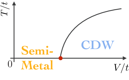
The paper is organized as follows: In Sec.2.1 we briefly review the CTQMC method with focuses on the absence of the sign problem [1]. In Sec. 2.2 we introduce the worm sampling technique in the Monte Carlo calculation [33, 34, 32] to improve the efficiency of the simulation. Section 3 contains our main results and discussions as well as comparisons with results obtained by infinite projected entangled-pair states (iPEPS) calculations. In Sec.4 we briefly anticipate several future research directions based on this work. In the appendix we provide technique details of our numerical calculation (A) and additional results obtained on the -flux square lattice (B).
2 Method
Two properties of the model (1) are essential for the absence of the sign problem in the CTQMC simulation. First, the filling is fixed at per site because of the particle-hole symmetry of the model. Second, the hopping matrix defined in Eq.(2) satisfies
| (4) |
where the “parity index” for a site sublattice.
2.1 Interaction expansion CTQMC and the sign problem
We expand the partition function of the system in terms of the interaction vertices of Eq.(3) [31, 32]
| (5) | |||||
where and is the partition function of the noninteracting system. denotes the average over the noninteracting Hamiltonian Eq.(2) and is the time ordering operator. The interaction vertices consist of pairs of neighboring sites. The delta functions in the first line of Eq.(5) indicates that the interactions are instantaneous. is a matrix
| (6) |
where is the noninteracting Green’s function. The particle-hole symmetry ensures that and therefore the diagonal element of vanishes. In addition, one has
| (7) |
while using the anti-periodicity of the Green’s function and Eq.(4) one has
| (8) |
Equations (6-8) show that the Green’s function matrix satisfies . Introducing a diagonal matrix , it can be written as
| (9) |
In other word, the matrix is skew-symmetric and its determinant is non-negative because it equals the square of the Pfaffian of the matrix. We will see in a moment that this ensures the absence of a sign problem in the CTQMC simulation.
We write Eq.(5) in a form suitable for Monte Carlo sampling
| (10) |
where denotes a configuration with vertices. Eq.(9) ensures that the weight 111The factor has been canceled by the permutations of the vertices. is always positive [1]
| (11) | |||||
In the second line we have used . The absence of a sign problem allows us to simulate fairly large systems at low temperatures to access the quantum critical point. In this paper, we simulate clusters with unit cells with periodic boundary conditions. The number of sites is . Close to the quantum critical point, nonrelativistic corrections are irrelevant and the dynamical critical exponent [10]. We thus scale the inverse temperature linearly with the system length . Because of the scaling of the CTQMC algorithm [31, 32], the largest system size considered in this paper is smaller than the one used in the projective auxiliary field QMC studies of the Hubbard model [19, 20, 21].
To detect the onset of the CDW order, we measure the density-density correlation function
| (12) |
where denotes the average over the full Hamiltonian Eq.(1). The second summation in Eq.(12) runs over all sites (in total of them) whose graph distance to the site is 222Strictly speaking, these sites may not be symmetrically related and may have slightly different correlation functions.. Two sites with even (odd) graph distance have the same (different) parities. The other two important observables are the square and quartic of the CDW order parameter
| (13) | |||||
| (14) |
The Binder ratio [35] is calculated as:
| (15) |
2.2 Worm Algorithm
Measuring and using the conventional approach [31] requires explicit loops over the indices and the measurements will dominate the runtime of Monte Carlo simulations. This is especially inefficient when noticing that each term in Eqs.(13-14) may differ by orders of magnitude. To overcome this difficulty we extend the configuration space and use the worm algorithm [33, 34, 32] to sample them efficiently.
| (16) | |||||
| (17) | |||||
where extends to the following matrix:
| (18) |
Similar to Eq.(9), satisfies the following equation
| (19) |
where the diagonal matrix extends in a similar manner. Similarly, is a matrix. We define , and enlarge the configuration space into
| (20) |
Now the configurations may contain a two site worm or a four site worm in addition to the vertices described in Eqs.(10). By sampling the extended configuration space we can treat the summation over in Eq.(16-17) and the summations over the vertices on an equal footing. Here and are two positive numbers we can choose freely to balance the configurations in different sectors. We have devised several Monte Carlo updates and describe them in A. We use the following notation to denote the relative time spend in the each sector [34]
| (21) | |||||
| (22) | |||||
| (23) |
The observables (13-15) then are
| (24) | |||||
| (25) | |||||
| (26) |
The density correlation function is measured when the configuration is in the space and the distance between the two worm sites is equal to ,
| (27) |
The weight of a configuration with worm at is
| (28) |
where we have used =. One can similarly show that the weight of sector is positive. Therefore, there is no sign problem in the extended configuration space with worms.
3 Results
3.1 Quantum Monte Carlo Results
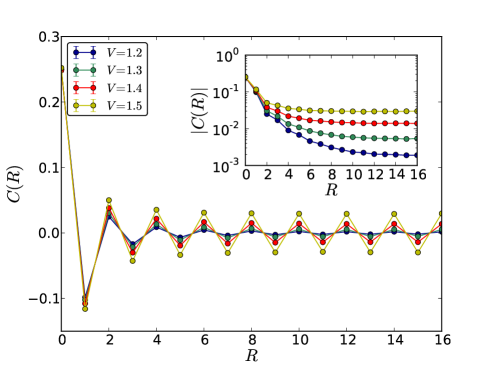
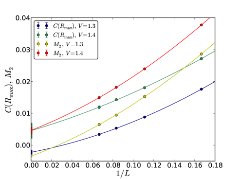
Figure 3 shows the density-density correlations (12), which develop a staggered pattern as the interaction strength increases. The density correlation at the farthest distance and the CDW structure factor approach the square of the CDW order parameter as the system size increases. Figure 4 shows the extrapolation of and to the thermodynamic limit using . The extrapolation suggests that the quantum critical point lies between and . 333The system sizes up to do not allow us to reliably pin down the critical point based on extrapolation [19, 20].
To better estimate the the critical point we perform a finite size scaling (FSS) analysis based on the scaling ansatz
| (29) | |||||
| (30) | |||||
| (31) |
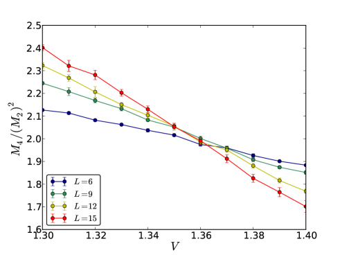
where and are universal functions and are the critical exponents. This scaling ansatz holds close to the critical point. The Binder ratios of different system sizes cross at the transition point. This provides a rough estimate of the transition point , as shown in Fig. 5.
-
1.356(1) 1.354(1) 1.356(2) 1.357(1) 0.80(3) 0.80(4) 0.83(8) 0.80(9) 0.302(7) 0.300(5) 0.298(2) 0.30(1) 0.52(2) 0.52(3) 0.44(5) 0.52(6) 1.23 2.05 1.4 1.61 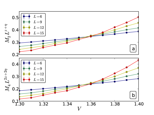

Figure 6: (a-b) The scaled and using . (c-d) Data collapse using and . We next collapse the data of and to determine the transition point and the critical exponents . The results are summarized in Table 3.1 where we also list the estimates of the order parameter critical exponent , which we will compare with iPEPS results in Sec.3.2. We have performed the data collapse using all available system sizes () and excluding the smallest system size (). They both give satisfactory data collapse where the per degree of freedom (d.o.f) is close to one. To visually examine the quality of the data collapse, Fig. 6(a-b) shows the scaled and using where all the curves intersect around . Further scale the horizontal axis using and collapse all the data onto a single curve, Fig.6(c-d).
Our estimation of the correlation length exponent agrees with earlier -expansion result [11] and functional renormalization group results [12, 13]. However, our estimated anomalous dimension is smaller than the previous estimates [11, 12, 13]. We have checked that these values of are not consistent with our QMC data. These field theory calculations [11, 12, 13] treated Dirac fermions with the same chiralities but our lattice model contains two Dirac fermions with opposite chirality. This difference might explain the discrepancies with our QMC data. On the other hand, since we observed subleading corrections in the Binder ratio crossing Fig. 5, further research using larger systems may be needed to determined the critical behavior more accurately.
3.2 Comparison with iPEPS Results
As an independent check of the results we have studied the model (1) with infinite projected entangled-pair states (iPEPS) - a variational tensor-network ansatz for two-dimensional ground-state wave functions in the thermodynamic limit [45, 46, 47, 48]. This ansatz is a natural extension of matrix product states (the underlying ansatz of the density-matrix renormalization group method) to two dimensions, and has been previously applied to the same model for attractive interactions [49, 50]. Two-dimensional tensor networks have first been introduced for spin models and later extended to fermionic systems [51, 52, 53, 54, 55, 56, 48, 57]. The iPEPS ansatz consists of a cell of tensors with one tensor per lattice site, which is periodically repeated on the lattice. Each tensor has a physical index of dimension which carries the local Hilbert space of a lattice site and auxiliary indices which connect to the nearest-neighboring tensors. The number of variational parameters (i.e. the accuracy of the ansatz) can be controlled by the bond dimension of the auxiliary indices, where each tensor contains variational parameters with and for the present model. For a general introduction to fermionic iPEPS we refer to Ref. [48].
We simulate the honeycomb model (1) by mapping it onto a brick-wall square lattice, as done in Ref. [58]. The variational parameters of the iPEPS ansatz are optimized by performing an imaginary time evolution using a second order Trotter-Suzuki decomposition and the full-update scheme for the truncation of a bond index (see Ref. [48] for details). To evaluate the iPEPS wave function (e.g. for the computation of expectation values) we use a variant of the corner-transfer-matrix method [59, 60] described in Refs. [61, 62]. The U(1) symmetry of the present model is exploited [63, 64] to increase the efficiency of the simulations.
Since iPEPS represent a wave function in the thermodynamic limit, symmetries of the Hamiltonian can be spontaneously broken, and the order can be measured by a local order parameter. In Fig. 7 the iPEPS results for the CDW order parameter as a function of is shown, where and correspond to the particle density on sublattices A and B, respectively. Since iPEPS is an ansatz in the thermodynamic limit, there are no finite size effects. However, the finite bond dimension has a similar effect on the order parameter as a finite size system, i.e. there is no sharp transition but the order parameter is overestimated around the critical coupling . To obtain an estimate of the order parameter in the infinite limit we extrapolate the data linearly in , shown by the black diamonds in Fig. 7. The error bar indicates the range of extrapolated values by taking into account different sets of data points. Although the analytical dependence of the order parameter on is not known, empirically, one can get a reasonable estimate by such type of extrapolations (see e.g. Ref [65]). Based on these extrapolations of the iPEPS data up to we obtain a value of the critical coupling of , in agreement with the CTQMC result.
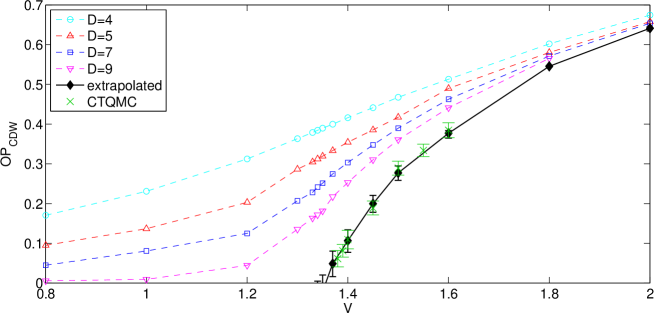
Figure 7: Results for the CDW order parameter as a function of repulsion strength obtained with iPEPS, compared to the extrapolated CTQMC data. The green crosses in Fig. 7 show the CTQMC data for the order parameter in the thermodynamic limit, computed as , which is in agreement with the iPEPS data. Similar results are obtained by estimating the order parameter from , i.e. . The extrapolation of QMC data close to the critical point is more difficult because the intersections at may become negative.
We also tried to extract the critical exponent by fitting the extrapolated iPEPS data to in the range . However, due to the error bars and sensitivity of the exponent on the fitting range we can only give a crude estimate of , which is somewhat larger than the CTQMC result , but both are smaller than the mean-field result [18] and consistent with the concave shape of the order parameter versus curve.
4 Conclusion and Outlook
We presented a sign problem free CTQMC study of the Dirac semi-metal to charge-density-wave transition on the honeycomb lattice and compare it with theory and iPEPS results. Our main results about the transition point and the critical exponents are summarized in the Table 3.1. The present study uses the static density-density correlations as the diagnosis tool for the quantum critical point, it is however interesting to further study the transport and entanglement properties across the phase transition. Future studies may map out the finite temperature phase diagram and especially the crossover [38] from the Gross-Neveu to the 2D Ising universality class. The CDW transition of the spinful Dirac fermions [39, 40] can also be studied using a similar method. Generalization of the model to include hopping and interactions beyond the nearest neighbors may allow us to address the intriguing question about the emergence [41] and stability of the topological insulating states [42, 43] in the presence of interactions.
The authors thank Igor Herbut, Kun Yang, Ziyang Meng, Su-Peng Kou, Hong Yao, Jakub Imriška, Jan Gukelberger and Hiroshi Shinaoka for useful discussions. Simulations were performed on the Mönch cluster of Platform for Advanced Scientific Computing (PASC), the Brutus cluster at ETH Zurich, and the “Monte Rosa” Cray XE6 at the Swiss National Supercomputing Centre (CSCS). We have used ALPS libraries [44] for Monte Carlo simulations and data analysis. This work was supported by ERC Advanced Grant SIMCOFE.Appendix A Monte Carlo Updates
A Monte Carlo update consists of proposing a move from a configuration to a new configuration with a priori probability . The acceptance probability satisfies the detailed balance condition
There are three classes of configurations shown in Fig. 8. We devised several updates to sample the configuration space. Most updates are in complementary pairs. Within each pair one can still fine tune the propose probability to enhance the acceptance rate.
Figure 8: The configuration space and the MC updates. A.1 Vertex add/remove
We add vertices to a configuration with vertices. The acceptance ratio is
(34) where is the number of bonds of the honeycomb lattice. The move Eq.(34) is balanced by removing vertices from a -vertices configuration with the acceptance probability
(35) Replace by one gets the formulas for adding/removing vertices in the worm space.
A.2 Worm creation/destruction
A.2.1
From the partition function sector we create a worm at . The corresponding new matrix is . To improve the acceptance rate, we select the site in the neighborhood (containing sites) of a randomly chosen site . The acceptance ratio is
(36) (37) A cheaper way to go between the partition function and the space is to randomly select a vertex and interpret it as a worm. We call this process an open update and the reverse process a close update. These two updates change the perturbation order by one. However they are cheaper than creating/destroying worms Eq.(36-37) because no matrix operation is involved. The acceptance ratios are
(38) (39) The factor accounts for the fact that and are counted as two distinct worm configurations.
A.2.2
In the sector we insert another worm at choosing a random site and a nearly site (out of sites). The time is the same as the imaginary time of the existing worm . Acceptance ratios are
(40) (41) A.2.3
We create a worm at in the partition function sector. To improve the acceptation ratio, we choose the sites in the neighborhood of a randomly chosen site . The ratios are
(42) (43) A.3 Worm shift
We shift the worm to a new space-time point. To enhance the acceptance probability, we randomly choose one site in the worm and shift it to one of its neighbors. The imaginary time is updated to by randomly by adding a random number in the range of . The matrix is updated to and the acceptance probability is
(44) This process is self-balanced. The acceptance rate of worm shift in the space has a similar expression.
Appendix B Monte Carlo results on the -flux lattice
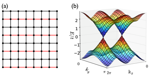
Figure 9: (a) A square lattice with -flux inserted to each plaquette. The hopping amplitude of the red bonds are , while on the black bonds . (b) The noninteracting band structure of the -flux lattice. To further confirm the critical exponent found in the main text, we simulated the model Eq.(1) on a square lattice with -flux inserted in each plaquette, Fig.9(a). The lattice also features two Dirac points in the Brillouin zone, Fig.9(b). The Dirac semimetal to CDW transition should belong to the same universality class in the honeycomb lattice. In the simulation we use the Landau gauge for the flux and choose system sizes to be divisible by . The inverse temperature scales linearly with length .
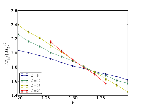
Figure 10: The Binder ratio Eq.(15) versus for different system sizes of the -flux lattice. Lines are linear interpolations of the data. 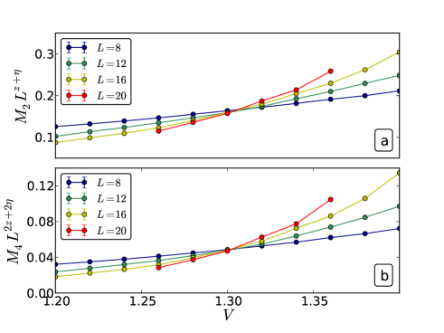
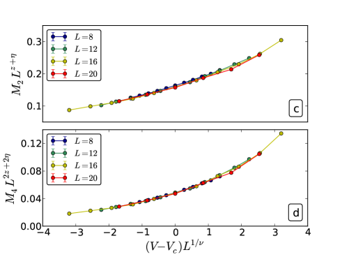
Figure 11: (a-b) The scaled and using . (c-d) Data collapse using and . References
References
- [1] Emilie Fulton Huffman and Shailesh Chandrasekharan. Solution to sign problems in half-filled spin-polarized electronic systems. Phys. Rev. B, 89(11):111101, March 2014.
- [2] A H Castro Neto, N M R Peres, K S Novoselov, and A K Geim. The electronic properties of graphene. Rev. Mod. Phys., 81(1):109–162, January 2009.
- [3] S Sachdev. Quantum Phase Transition. Cambridge Univ. Press, 2011.
- [4] M Z Hasan and C L Kane. Colloquium: Topological insulators. Rev. Mod. Phys., 82(4):3045–3067, November 2010.
- [5] Thomas Uehlinger, Gregor Jotzu, Michael Messer, Daniel Greif, Walter Hofstetter, Ulf Bissbort, and Tilman Esslinger. Artificial Graphene with Tunable Interactions. Phys. Rev. Lett., 111(18):185307, October 2013.
- [6] Baruch Rosenstein, Brian J Warr, and Seon H Park. Dynamical symmetry breaking in four-fermion interaction models. Physics Reports, 205(2):59–108, 1991.
- [7] David J Gross and Andre Neveu. Dynamical symmetry breaking in asymptotically free field theories. Phys. Rev. D, 10(10):3235, 1974.
- [8] Igor F Herbut. Interactions and Phase Transitions on Graphene’s Honeycomb Lattice. Phys. Rev. Lett., 97(14):146401, October 2006.
- [9] Igor Herbut, Vladimir Juričić, and Oskar Vafek. Relativistic Mott criticality in graphene. Phys. Rev. B, 80(7):075432, August 2009.
- [10] Igor F Herbut, Vladimir Juričić, and Bitan Roy. Theory of interacting electrons on the honeycomb lattice. Phys. Rev. B, 79(8):085116, February 2009.
- [11] B Rosenstein, Hoi-Lai Yu, and A Kovner. Critical exponents of new universality classes. Physics Letters B, 314(3):381–386, 1993.
- [12] L Rosa, P Vitale, and C Wetterich. Critical Exponents of the Gross-Neveu Model from the Effective Average Action. Phys. Rev. Lett., 86(6):958–961, February 2001.
- [13] F Höfling, C Nowak, and C Wetterich. Phase transition and critical behavior of the d=3 Gross-Neveu model. Phys. Rev. B, 66(20):205111, November 2002.
- [14] R B Laughlin. Magnetic Induction of d x 2-y 2+ id xy Order in High-T c Superconductors. Phys. Rev. Lett., 80(23):5188, 1998.
- [15] Matthias Vojta, Ying Zhang, and Subir Sachdev. Quantum phase transitions in d-wave superconductors. Phys. Rev. Lett., 85(23):4940, 2000.
- [16] D Khveshchenko and J Paaske. Incipient Nodal Pairing in Planar d-wave Superconductors. Phys. Rev. Lett., 86(20):4672–4675, May 2001.
- [17] Matthias Troyer and Uwe-Jens Wiese. Computational Complexity and Fundamental Limitations to Fermionic Quantum Monte Carlo Simulations. Phys. Rev. Lett., 94(17):170201, May 2005.
- [18] S Sorella and E Tosatti. Semi-metal-insulator transition of the Hubbard model in the honeycomb lattice. EPL, 19(8):699, 1992.
- [19] Z Y Meng, T C Lang, S Wessel, F F Assaad, and A Muramatsu. Quantum spin liquid emerging in two-dimensional correlated Dirac fermions. Nature, 464(7290):847–851, August 2010.
- [20] Sandro Sorella, Yuichi Otsuka, and Seiji Yunoki. Absence of a Spin Liquid Phase in the Hubbard Model on the Honeycomb Lattice. Sci. Rep., 2, December 2012.
- [21] Fakher F Assaad and Igor F Herbut. Pinning the Order: The Nature of Quantum Criticality in the Hubbard Model on Honeycomb Lattice. Phys. Rev. X, 3(3):031010, August 2013.
- [22] R Blankenbecler, D J Scalapino, and R L Sugar. Monte Carlo calculations of coupled boson-fermion systems. I. Phys. Rev. D, 24(8):2278, 1981.
- [23] D J Scalapino, R L Sugar, and W D Toussaint. Monte Carlo study of a two-dimensional spin-polarized fermion lattice gas. Phys. Rev. B, 29(9):5253, 1984.
- [24] J E Gubernatis, D J Scalapino, R L Sugar, and W D Toussaint. Two-dimensional spin-polarized fermion lattice gases. Phys. Rev. B, 32(1):103, 1985.
- [25] Shailesh Chandrasekharan and Uwe-Jens Wiese. Meron-cluster solution of fermion sign problems. Phys. Rev. Lett., 83(16):3116, 1999.
- [26] S Chandrasekharan, J Cox, K Holland, and U J Wiese. Meron-cluster simulation of a chiral phase transition with staggered fermions. Nuclear Physics B, 576(1):481–500, 2000.
- [27] J Cox and K Holland. Meron-cluster algorithms and chiral-symmetry breaking in a (2+ 1) D staggered fermion model. Nuclear Physics B, 583(1):331–346, 2000.
- [28] Shailesh Chandrasekharan. Fermion bag approach to lattice field theories. Phys. Rev. D, 82(2):025007, July 2010.
- [29] Shailesh Chandrasekharan and Anyi Li. Fermion Bags, Duality, and the Three Dimensional Massless Lattice Thirring Model. Phys. Rev. Lett., 108(14):140404, April 2012.
- [30] Shailesh Chandrasekharan and Anyi Li. Quantum critical behavior in three dimensional lattice Gross-Neveu models. Phys. Rev. D, 88(2):021701, July 2013.
- [31] A Rubtsov, V Savkin, and A Lichtenstein. Continuous-time quantum Monte Carlo method for fermions. Phys. Rev. B, 72(3):035122, July 2005.
- [32] Emanuel Gull, Andrew J Millis, Alexander I Lichtenstein, Alexey N Rubtsov, Matthias Troyer, and Philipp Werner. Continuous-time Monte Carlo methods for quantum impurity models. Rev. Mod. Phys., 83(2):349–404, May 2011.
- [33] N V Prokof’ev, Svistunov, BV, and I S Tupitsyn. Exact, complete, and universal continuous-time worldline Monte Carlo approach to the statistics of discrete quantum systems. Journal of Experimental and Theoretical Physics, 87(2):310–321, 1998.
- [34] Evgeni Burovski, Nikolay Prokof’ev, Boris Svistunov, and Matthias Troyer. The Fermi–Hubbard model at unitarity. New J. Phys., 8(8):153–153, August 2006.
- [35] Kurt Binder. Finite size scaling analysis of Ising model block distribution functions. Zeitschrift für Physik B Condensed Matter, 43(2):119–140, 1981.
- [36] Jérôme Houdayer and Alexander Hartmann. Low-temperature behavior of two-dimensional Gaussian Ising spin glasses. Phys. Rev. B, 70(1):014418, July 2004.
- [37] O Melchert. autoScale.py - A program for automatic finite-size scaling analyses: A user’s guide. arXiv, physics.comp-ph, October 2009.
- [38] J Cardy. Scaling and Renormalization in Statistical Physic. Cambridge Univ. Press, 1996.
- [39] Carsten Honerkamp. Density Waves and Cooper Pairing on the Honeycomb Lattice. Phys. Rev. Lett., 100(14):146404, April 2008.
- [40] Wei Wu and A.-M. S. Tremblay. Phase diagram and fermi liquid properties of the extended hubbard model on the honeycomb lattice. Phys. Rev. B, 89:205128, May 2014.
- [41] S Raghu, Xiao-Liang Qi, C Honerkamp, and Shou-Cheng Zhang. Topological Mott Insulators. Phys. Rev. Lett., 100(15):156401, April 2008.
- [42] Christopher N Varney, Kai Sun, Marcos Rigol, and Victor Galitski. Interaction effects and quantum phase transitions in topological insulators. Phys. Rev. B, 82(11):115125, September 2010.
- [43] Christopher N Varney, Kai Sun, Marcos Rigol, and Victor Galitski. Topological phase transitions for interacting finite systems. Phys. Rev. B, 84(24):241105, December 2011.
- [44] B Bauer, L D Carr, H G Evertz, A Feiguin, J Freire, E Gull, S Fuchs, L Gamper, J Gukelberger, Guertler S, A Hehn, R Igarashi, SV Isakov, D Koop, PN Ma, P Mates, H Matsuo, O Parcollet, G Pawlowski, JD Picon, L Pollet, E Santos, VW Scarola, U Schollwoeck, C Silva, B Surer, S Todo, S Trebst, M Troyer, ML Wall, P Werner, and S Wessel. The ALPS project release 2.0: open source software for strongly correlated systems. J. Stat. Mech.: Theor. Exp., 2011(05):P05001, 2011.
- [45] F. Verstraete and J. I. Cirac. Renormalization algorithms for Quantum-Many Body Systems in two and higher dimensions. Preprint, 2004.
- [46] F. Verstraete, V. Murg, and J. I. Cirac. Matrix product states, projected entangled pair states, and variational renormalization group methods for quantum spin systems. Advances in Physics, 57(2):143, 2008.
- [47] J. Jordan, R. Orús, G. Vidal, F. Verstraete, and J. I. Cirac. Classical Simulation of Infinite-Size Quantum Lattice Systems in Two Spatial Dimensions. Phys. Rev. Lett., 101(25):250602, 2008.
- [48] P. Corboz, R. Orus, B. Bauer, and G. Vidal. Simulation of strongly correlated fermions in two spatial dimensions with fermionic projected entangled-pair states. Phys. Rev. B, 81:165104, 2010.
- [49] P. Corboz, S. Capponi, A. M. Läuchli, B. Bauer, and R. Orús. Comment on “Topological quantum phase transitions of attractive spinless fermions in a honeycomb lattice” by poletti d. et al. EPL (Europhys. Lett.), 98(2):27005, April 2012.
- [50] Zheng-Cheng Gu. Efficient simulation of grassmann tensor product states. Phys. Rev. B, 88(11):115139, September 2013.
- [51] P. Corboz, G. Evenbly, F. Verstraete, and G. Vidal. Simulation of interacting fermions with entanglement renormalization. Phys. Rev. A, 81:010303(R), 2010.
- [52] Christina V. Kraus, Norbert Schuch, Frank Verstraete, and J. Ignacio Cirac. Fermionic projected entangled pair states. Phys. Rev. A, 81:052338, 2010.
- [53] Carlos Pineda, Thomas Barthel, and Jens Eisert. Unitary circuits for strongly correlated fermions. Phys. Rev. A, 81(5):050303, May 2010.
- [54] T. Barthel, C. Pineda, and J. Eisert. Contraction of fermionic operator circuits and the simulation of strongly correlated fermions. Phys. Rev. A, 80:042333, 2009.
- [55] Q.-Q. Shi, S.-H. Li, J.-H. Zhao, and H.-Q. Zhou. Graded Projected Entangled-Pair State Representations and An Algorithm for Translationally Invariant Strongly Correlated Electronic Systems on Infinite-Size Lattices in Two Spatial Dimensions. Preprint, 2009.
- [56] P. Corboz and G. Vidal. Fermionic multi-scale entanglement renormalization ansatz. Phys. Rev. B, 80:165129, 2009.
- [57] Z.-C. Gu, F. Verstraete, and X.-G. Wen. Grassmann tensor network states and its renormalization for strongly correlated fermionic and bosonic states. Preprint, 2010.
- [58] Philippe Corboz, Miklós Lajkó, Andreas M. Läuchli, Karlo Penc, and Frédéric Mila. Spin-orbital quantum liquid on the honeycomb lattice. Phys. Rev. X, 2(4):041013, November 2012.
- [59] Tomotoshi Nishino and Kouichi Okunishi. Corner Transfer Matrix Renormalization Group Method. J. Phys. Soc. Jpn., 65(4):891–894, 1996.
- [60] Román Orús and Guifré Vidal. Simulation of two-dimensional quantum systems on an infinite lattice revisited: Corner transfer matrix for tensor contraction. Phys. Rev. B, 80:094403, 2009.
- [61] P. Corboz, S.R. White, G. Vidal, and M. Troyer. Stripes in the two-dimensional t-J model with infinite projected entangled-pair states. Phys. Rev. B, 84(4):041108, 2011.
- [62] Philippe Corboz, T. M. Rice, and Matthias Troyer. Competing states in the t-j model: uniform d-wave state versus stripe state. arXiv:1402.2859 [cond-mat], February 2014.
- [63] Sukhwinder Singh, Robert N. C. Pfeifer, and Guifre Vidal. Tensor network states and algorithms in the presence of a global U(1) symmetry. Phys. Rev. B, 83(11):115125, 2011.
- [64] B. Bauer, P. Corboz, R. Orús, and M. Troyer. Implementing global abelian symmetries in projected entangled-pair state algorithms. Phys. Rev. B, 83(12):125106, 2011.
- [65] Philippe Corboz and Frédéric Mila. Tensor network study of the shastry-sutherland model in zero magnetic field. Phys. Rev. B, 87(11):115144, March 2013.