DESY 14-041
IFT-UAM/CSIC-14-058
Neutralinos betray their singlino nature at the ILC

Gudrid Moortgat-Pick111gudrid.moortgat-pick@desy.de II. Institut für Theoretische Physik, University of Hamburg, Germany DESY, Hamburg, Germany Stefano Porto222stefano.porto@desy.de II. Institut für Theoretische Physik, University of Hamburg, Germany Krzysztof Rolbiecki333krzysztof.rolbiecki@desy.de Instituto de Fisica Teorica IFT-UAM/CSIC, Madrid, Spain
Abstract

It is one of the most challenging tasks at the Large Hadron Collider and at a future Linear Collider not only to observe physics beyond the Standard Model, but to clearly identify the underlying new physics model. In this paper we concentrate on the distinction between two different supersymmetric models, the MSSM and the NMSSM, as they can lead to similar low energy spectra. The NMSSM adds a singlet superfield to the MSSM particle spectrum and simplifies embedding a SM-like Higgs candidate with the measured mass of about 125.5 GeV. In parts of the parameter space the Higgs sector itself does not provide sufficient indications for the underlying model. We show that exploring the gaugino/higgsino sectors could provide a meaningful way to distinguish the two models. Assuming that only the lightest chargino and neutralino masses and polarized cross sections e+eχ~i0χ~j0superscript𝑒superscript𝑒subscriptsuperscript~𝜒0𝑖subscriptsuperscript~𝜒0𝑗e^{+}e^{-}\to\tilde{\chi}^{0}_{i}\tilde{\chi}^{0}_{j}, χ~i+χ~jsubscriptsuperscript~𝜒𝑖subscriptsuperscript~𝜒𝑗\tilde{\chi}^{+}_{i}\tilde{\chi}^{-}_{j} are accessible at the linear collider, we reconstruct the fundamental MSSM parameters M1subscript𝑀1M_{1}, M2subscript𝑀2M_{2}, μ𝜇\mu, tanβ𝛽\tan\beta and study whether a unique model distinction is possible based on this restricted information. Depending on the singlino admixture in the lightest neutralino states, as well as their higgsino or gaugino nature, we define several classes of scenarios and study the prospects of experimental differentiation.

1 Introduction

The discovery of a neutral scalar particle [1, 2] with mass 125.5similar-toabsent125.5\sim 125.5 GeV at the Large Hadron Collider (LHC) [3, 4] has opened a plethora of discussions about its identity. While the experimental uncertainty suggests the new particle to be the Standard Model Higgs boson, more data are still needed to precisely determine its branching ratios, the CP properties and the underlying model. The present results are in fact compatible with one of the most promising Beyond the Standard Model candidates: supersymmetry (SUSY) [5]. The latter solves — contrary to the Standard Model (SM) — the electroweak hierarchy puzzle, offers a dark matter candidate and is consistent with grand unification of the gauge couplings.

The most studied supersymmetric models are the Minimal Supersymmetric Standard Model (MSSM) [5] and its minimal extension, the Next-to-Minimal Supersymmetric Standard Model (NMSSM) [6]. The NMSSM introduces a gauge singlet chiral supermultiplet S~~𝑆\tilde{S} that allows for a relaxation of the electroweak fine tuning conditions, compared to the MSSM. On the other hand, the — so far — negative result of LHC searches for physics beyond the Standard Model (BSM) [7, 8] does not favor any of these models a priori.

In case of SUSY discovery at the LHC and/or at a linear collider (LC) it is therefore important to understand how to entail the underlying supersymmetric model, in particular how to distinguish between NMSSM and MSSM. These two models have indeed a very similar particle spectrum, with the exception for the superfield S^^𝑆\hat{S} in the NMSSM that results in three additional states with respect to the MSSM: a CP-even Higgs, a CP-odd Higgs and a fifth neutralino.

It is therefore well-motivated to look at the Higgs sector, where the experiments are expected to give the most precise indications [9, 10], and to complement the information by studying the (extended) neutralino sector of the NMSSM to look for deviations with respect to the MSSM.

Concerning the gaugino/higgsino sector, it has been shown that detecting the lightest chargino χ~1±subscriptsuperscript~𝜒plus-or-minus1\tilde{\chi}^{\pm}_{1} [11], and neutralino states χ~10subscriptsuperscript~𝜒01\tilde{\chi}^{0}_{1}, χ~20subscriptsuperscript~𝜒02\tilde{\chi}^{0}_{2} [12, 13], a full reconstruction of the MSSM chargino and neutralino sectors through χ2superscript𝜒2\chi^{2}-fits [14, 15], is possible based on measuring the masses and their polarized cross sections. A fit disfavouring the MSSM suggests to look at minimal extensions that modify the neutralino/chargino sector, in primis the NMSSM [16, 17].

In fact, the singlino admixtures of neutralino lightest states as well as the higgsino and gaugino components of χ~10superscriptsubscript~𝜒10\tilde{\chi}_{1}^{0} allow to identify several classes of NMSSM scenarios. Scenarios where the singlino component in the light neutralinos is significant (light singlino scenarios), are often treated in the literature, featuring production cross sections and phenomenology different from the MSSM and are in principle easier to spot. If the singlino, however, is heavy and mainly present in χ~30superscriptsubscript~𝜒30\tilde{\chi}_{3}^{0}, χ~40superscriptsubscript~𝜒40\tilde{\chi}_{4}^{0} or χ~50superscriptsubscript~𝜒50\tilde{\chi}_{5}^{0}, the phenomenology is more MSSM-like and we distinguish the cases where the main component of the lightest χ~10superscriptsubscript~𝜒10\tilde{\chi}_{1}^{0} is higgsino-like (light higgsino scenarios) or gaugino-like (light gaugino scenarios). Having a decoupled singlino may result in a scenario that is experimentally not distinguishable from the MSSM without further information about the heavier neutralino states and the Higgs sector. Our analysis confirms these hints, concluding that a light and accessible singlino is one of the most efficient ways for model distinction together with a light singlet scalar.

The paper is organized in the following way: first we introduce our proposed strategy to discriminate the different models in section 2 and describe the classes of scenarios in section 3. In that section we also try to clearly classify in which cases a unique distinction between both models is possible based only on the light electroweak states and to work out which further information is required in cases where the light sector alone does not provide sufficient information for a model discrimination. Therefore we perform scans in the (λ,κ)𝜆𝜅(\lambda,\,\kappa)-plane, applying the most recent phenomenological and experimental constraints from colliders, including also dark matter experiments, and determine where the singlino admixtures are such that the NMSSM cannot be misinterpreted as MSSM. We summarize our results in 4 and list details and parameters on the models in the appendices A, B.

2 Strategy

As explained in the Introduction, the NMSSM adds to the MSSM an additional gauge singlet superfield S^^𝑆\hat{S} in the Higgs sector. The most studied version of the NMSSM has a Lagrangian with an accidental 3subscript3\mathbb{Z}_{3} symmetry, obtained from the scale invariant superpotential [6]

W3-NMSSMλS^H^uH^d+κ3S^3.𝜆^𝑆subscript^𝐻𝑢subscript^𝐻𝑑𝜅3superscript^𝑆3subscript𝑊subscript3-NMSSMW_{\tiny\mathbb{Z}_{3}\mbox{-NMSSM}}\supset\lambda\,\hat{S}\hat{H}_{u}\cdot\hat{H}_{d}+\frac{\kappa}{3}\,\hat{S}^{3}\,. (1)

S^^𝑆\hat{S} consists of a scalar Higgs singlet S𝑆S and the singlino S~~𝑆\tilde{S}. The additional dimensional parameters Aλsubscript𝐴𝜆A_{\lambda} and Aκsubscript𝐴𝜅A_{\kappa} appear in the Higgs sector soft terms:

soft,3-NMSSMλAλHuHdS13AκS3.𝜆subscript𝐴𝜆subscript𝐻𝑢subscript𝐻𝑑𝑆13subscript𝐴𝜅superscript𝑆3subscriptsoftsubscript3-NMSSM\mathcal{L}_{\tiny\rm soft,\mathbb{Z}_{3}\mbox{-NMSSM}}\supset-\lambda A_{\lambda}H_{u}\cdot H_{d}S-\frac{1}{3}A_{\kappa}S^{3}. (2)

The singlet S𝑆S, see Eqs. (1) and (2), mixes due to the electroweak symmetry breaking with the MSSM Higgs doublets Hu,Hdsubscript𝐻𝑢subscript𝐻𝑑H_{u},\,H_{d}, resulting in three CP-even neutral scalars h1,h2,h3subscript1subscript2subscript3h_{1},\,h_{2},\,h_{3} and two CP-odd neutral scalars a1,a2subscript𝑎1subscript𝑎2a_{1},\,a_{2}. Correspondingly, the singlino S~~𝑆\tilde{S} mixes with the higgsinos and the gauginos, resulting in five neutralino mass eigenstates. Therefore, determining the nature of weakly coupling scalars or neutralinos is the first way to discriminate between NMSSM and MSSM.

In the light of the expected high accuracy in the Higgs sector measurements [10], it is a common practice to compare MSSM and NMSSM scenarios looking at the Higgs sector, in particular at the Higgs decays [18, 19, 20]. The case in which a very light CP-even and/or a light CP-odd scalars have high singlet component and allow new decay channels for the SM-like Higgs scalar affecting its decay width and branching ratios has been explored [21]. On the same footing, looking at the extended NMSSM neutralino sector is very well motivated, especially for linear collider phenomenology, due to the high precision in the electroweak sector. This can be crucial in case of relatively heavy singlet states in comparison with the SM-like Higgs, such that the observed Higgs sector can be interpreted within both the MSSM and the NMSSM. In such scenarios with heavy decoupled states, the corresponding signatures at the LHC would indeed be very similar in both models [10].

We are therefore interested to understand how much information can be obtained from the neutralino and chargino sector for the model distinction. In the MSSM, the parameters M1subscript𝑀1M_{1}, M2subscript𝑀2M_{2}, μ𝜇\mu, tanβ𝛽\tan\beta fully describe the chargino and neutralino sector. One should note that these are fundamental parameters without any assumption on the SUSY breaking scheme. Precise determination of these parameters is possible at a linear collider [11, 12, 13, 14, 22], provided that χ~10subscriptsuperscript~𝜒01\tilde{\chi}^{0}_{1}, χ~20subscriptsuperscript~𝜒02\tilde{\chi}^{0}_{2} and χ~1±subscriptsuperscript~𝜒plus-or-minus1\tilde{\chi}^{\pm}_{1} can be produced at the LC and their masses as well as the polarized cross sections σ(e+eχ~10χ~20)𝜎superscript𝑒superscript𝑒subscriptsuperscript~𝜒01subscriptsuperscript~𝜒02\sigma(e^{+}e^{-}\rightarrow\tilde{\chi}^{0}_{1}\tilde{\chi}^{0}_{2}), σ(e+eχ~1+χ~1)𝜎superscript𝑒superscript𝑒subscriptsuperscript~𝜒1subscriptsuperscript~𝜒1\sigma(e^{+}e^{-}\rightarrow\tilde{\chi}^{+}_{1}\tilde{\chi}^{-}_{1}) are measured. An accurate and rather model-independent determination of M1subscript𝑀1M_{1}, M2subscript𝑀2M_{2}, μ𝜇\mu, tanβ𝛽\tan\beta is performed by a χ2superscript𝜒2\chi^{2}-minimisation that selects the parameters fitting the experimental results. Such analysis can be strengthened if the mass of the heavier neutralino states can be inferred from combined analyses of LHC and LC data [14].

The possibility of reconstructing the MSSM chargino-neutralino sector parameters can then be exploited as a tool for the distinction between the MSSM and the NMSSM [16]. Given experimental observation of χ~10subscriptsuperscript~𝜒01\tilde{\chi}^{0}_{1}, χ~20subscriptsuperscript~𝜒02\tilde{\chi}^{0}_{2} and χ~1±subscriptsuperscript~𝜒plus-or-minus1\tilde{\chi}^{\pm}_{1}, a result of the χ2superscript𝜒2\chi^{2}-fit that excludes the MSSM at 95% confidence level (C.L.), may suggest the NMSSM. It has indeed been shown [16] that relatively different mixing for MSSM and NMSSM scenarios can lead to very similar neutralino and chargino mass spectra in both models; this is of course also true in case of a scenarios with similar soft parameters and a decoupled singlet superfield.

Following this idea, we outline our strategy:

  • Scenario selection. We identify NMSSM scenarios that present a mass spectrum for χ~1±subscriptsuperscript~𝜒plus-or-minus1\tilde{\chi}^{\pm}_{1}, χ~10subscriptsuperscript~𝜒01\tilde{\chi}^{0}_{1}, χ~20subscriptsuperscript~𝜒02\tilde{\chi}^{0}_{2} and low Higgs spectrum that can be attributed also to a MSSM scenario. We calculate the corresponding NMSSM neutralino and chargino tree-level masses and polarized cross-sections for the processes e+eχ~1+χ~1superscript𝑒superscript𝑒subscriptsuperscript~𝜒1subscriptsuperscript~𝜒1e^{+}e^{-}\rightarrow\tilde{\chi}^{+}_{1}\tilde{\chi}^{-}_{1} and e+eχ~10χ~20superscript𝑒superscript𝑒subscriptsuperscript~𝜒01subscriptsuperscript~𝜒02e^{+}e^{-}\rightarrow\tilde{\chi}^{0}_{1}\tilde{\chi}^{0}_{2} cf. (Figures 1 and 2).

  • Constraints. Each scenario has to fulfill a series of phenomenological and experimental constraints implemented in NMSSMTools-4.2.1, that includes NMHDECAY [23, 24, 25] and NMSDECAY [26, 27]. These tools calculate the Higgs sector parameters, SUSY particle masses at the loop level and their decays, and confront them with limits from LEP, LHC and EW precision constraints. An interface to MicrOMEGAS [28] provides dark matter constraints, including the latest LUX [29] and Planck [30] results. The LSP relic density is required to be ΩLSPh2<0.131subscriptΩLSPsuperscript20.131\Omega_{\rm LSP}h^{2}<0.131, where hh is the Hubble constant in units of 100 km/(s\cdotMpc). Higgs sector constraints are further controlled using HiggsBounds-4.0.0 [31] and HiggsSignals-1.0.0 [32], such that a scenario is accepted only if compatible with current data at the 95% (C.L.).

  • Experimental assumption. We assume, for each NMSSM scenario, an observation of χ~1±subscriptsuperscript~𝜒plus-or-minus1\tilde{\chi}^{\pm}_{1}, χ~10subscriptsuperscript~𝜒01\tilde{\chi}^{0}_{1} and χ~20subscriptsuperscript~𝜒02\tilde{\chi}^{0}_{2} at the ILC together with their total cross sections σ(e+eχ~1+χ~1)𝜎superscript𝑒superscript𝑒subscriptsuperscript~𝜒1subscriptsuperscript~𝜒1\sigma(e^{+}e^{-}\rightarrow\tilde{\chi}^{+}_{1}\tilde{\chi}^{-}_{1}), σ(e+eχ~10χ~20)𝜎superscript𝑒superscript𝑒subscriptsuperscript~𝜒01subscriptsuperscript~𝜒02\sigma(e^{+}e^{-}\rightarrow\tilde{\chi}^{0}_{1}\tilde{\chi}^{0}_{2}) with electron-positron beam polarizations (𝒫e,𝒫e+)=(±0.9,0.55)subscript𝒫superscript𝑒subscript𝒫superscript𝑒plus-or-minus0.9minus-or-plus0.55(\mathcal{P}_{e^{-}},\mathcal{P}_{e^{+}})=(\pm 0.9,\mp 0.55) at s=350𝑠350\sqrt{s}=350 GeV (corresponding to the tt¯𝑡¯𝑡t\bar{t}-threshold) and at s=500𝑠500\sqrt{s}=500 GeV. A precision of 0.5% on the masses and 1% on the cross sections is assumed [33, 34]. If kinematically accessible, also mχ~30subscript𝑚subscriptsuperscript~𝜒03m_{\tilde{\chi}^{0}_{3}}, and the processes e+eχ~10χ~30superscript𝑒superscript𝑒subscriptsuperscript~𝜒01subscriptsuperscript~𝜒03e^{+}e^{-}\rightarrow\tilde{\chi}^{0}_{1}\tilde{\chi}^{0}_{3}, e+eχ~20χ~30superscript𝑒superscript𝑒subscriptsuperscript~𝜒02subscriptsuperscript~𝜒03e^{+}e^{-}\rightarrow\tilde{\chi}^{0}_{2}\tilde{\chi}^{0}_{3} are considered.

  • χ𝟐superscript𝜒2\mathbf{\chi^{2}}-fit to MSSM. The measured quantities and errors are used to perform a MSSM parameter determination through the χ2superscript𝜒2\chi^{2}-fit following the recipe in [14], similarly to [16]. We apply the χ2superscript𝜒2\chi^{2}-fit using Minuit [35], that minimizes the χ2superscript𝜒2\chi^{2} function defined as

    χ2=i|𝒪i𝒪¯iδ𝒪i|2,superscript𝜒2subscript𝑖superscriptsubscript𝒪𝑖subscript¯𝒪𝑖𝛿subscript𝒪𝑖2,\chi^{2}=\sum_{i}\left|\frac{\mathcal{O}_{i}-\bar{\mathcal{O}}_{i}}{\delta\mathcal{O}_{i}}\right|^{2}\mbox{,} (3)

    where 𝒪isubscript𝒪𝑖\mathcal{O}_{i} are the input observables, δOi𝛿subscript𝑂𝑖\delta O_{i} are the associated experimental uncertainties and O¯isubscript¯𝑂𝑖\bar{O}_{i} are the theoretical values of the observables calculated using the fitted MSSM parameters. The unknowns of the fit will be M1,M2,μ,tanβsubscript𝑀1subscript𝑀2𝜇𝛽M_{1},\,M_{2},\,\mu,\,\tan\beta and mν~esubscript𝑚subscript~𝜈𝑒m_{\tilde{\nu}_{e}}.444The mass mν~esubscript𝑚subscript~𝜈𝑒m_{\tilde{\nu}_{e}} is related to the selectron masses by applying the SU(2) relation mν~e2=me~L2+cos(2β)cos2θWmZ2superscriptsubscript𝑚subscript~𝜈𝑒2superscriptsubscript𝑚subscript~𝑒𝐿22𝛽superscript2subscript𝜃𝑊superscriptsubscript𝑚𝑍2m_{\tilde{\nu}_{e}}^{2}=m_{\tilde{e}_{L}}^{2}+\cos(2\beta)\cos^{2}\theta_{W}m_{Z}^{2} and me~L=me~Rsubscript𝑚subscript~𝑒𝐿subscript𝑚subscript~𝑒𝑅m_{\tilde{e}_{L}}=m_{\tilde{e}_{R}}. In the case of high tanβ𝛽\tan\beta, its extraction could be difficult, and only a lower limit could be set. A fit that is not consistent with the MSSM 95% C.L., may give hints towards the NMSSM and model distinction. If this is not the case, more information is needed to be included to establish the nature of the observed model. The limiting (95% C.L.) value of χ2superscript𝜒2\chi^{2} varies for different scenarios under consideration depending on the number of observables used in the fit.

  • Information from the Higgs sector. If the singlet is relatively light and has a substantial mixing with the SM-like Higgs, one could observe deviations from the SM predictions that cannot be accommodated within the MSSM at the same time. In our case, we expect small departure from the SM values and we limit ourselves to comparing the NMSSM predictions to the SM model by doing a χ2superscript𝜒2\chi^{2}-fit of the reduced couplings of the SM-like Higgs to g,γ,W,Z,b,c,τ𝑔𝛾𝑊𝑍𝑏𝑐𝜏g,\gamma,W,Z,b,c,\tau. If the couplings do not differ too much from the SM, such a scenario could always be accommodated within the MSSM in the decoupling limit as well. Alternatively, one could consider a possibility of detection additional singlet-like states, but this analysis is beyond the scope of the current paper.

Refer to caption
Figure 1: Chargino tree-level production channels at e+esuperscript𝑒superscript𝑒e^{+}e^{-} colliders.
Refer to caption
Figure 2: Neutralino tree-level production channels at e+esuperscript𝑒superscript𝑒e^{+}e^{-} colliders.

3 Classes of scenarios

The singlino (S~~𝑆\tilde{S}) admixtures of the lightest neutralino states χ~10subscriptsuperscript~𝜒01\tilde{\chi}^{0}_{1} and χ~20subscriptsuperscript~𝜒02\tilde{\chi}^{0}_{2} suggest the classification of NMSSM scenarios with the following limiting cases:

  1. 1.

    Light singlino (LS) scenarios: high S~~𝑆\tilde{S} admixture in the light states χ~10subscriptsuperscript~𝜒01\tilde{\chi}^{0}_{1} or χ~20subscriptsuperscript~𝜒02\tilde{\chi}^{0}_{2}.

  2. 2.

    Light higgsino (LH) scenarios: higgsino-like χ~10subscriptsuperscript~𝜒01\tilde{\chi}^{0}_{1}, with μeff<M1,M2subscript𝜇effsubscript𝑀1subscript𝑀2\mu_{\rm eff}<M_{1},M_{2} and high S~~𝑆\tilde{S} admixture mainly in χ~30,χ~40,χ~50subscriptsuperscript~𝜒03subscriptsuperscript~𝜒04subscriptsuperscript~𝜒05\tilde{\chi}^{0}_{3},\tilde{\chi}^{0}_{4},\tilde{\chi}^{0}_{5}.

  3. 3.

    Light gaugino (LG) scenarios: gaugino-like χ~10subscriptsuperscript~𝜒01\tilde{\chi}^{0}_{1}, with μeff>M1,M2subscript𝜇effsubscript𝑀1subscript𝑀2\mu_{\rm eff}>M_{1},M_{2} and high S~~𝑆\tilde{S} admixture mainly in χ~30,χ~40,χ~50subscriptsuperscript~𝜒03subscriptsuperscript~𝜒04subscriptsuperscript~𝜒05\tilde{\chi}^{0}_{3},\tilde{\chi}^{0}_{4},\tilde{\chi}^{0}_{5}.

Exploring these classes of scenarios allows to embed also the intermediate cases of mixed lightest neutralino nature.

A high singlino admixture in χ~10subscriptsuperscript~𝜒01\tilde{\chi}^{0}_{1} and/or χ~20subscriptsuperscript~𝜒02\tilde{\chi}^{0}_{2} as in case 1 may signal beyond-MSSM physics. A fit reconstructing the higgsino and gaugino components hypothesizing MSSM would give very different result with respect to the original NMSSM. In such a case, the outlined strategy for model distinction seems promising, see [16] and section 3.1, as different gaugino and neutralino admixtures lead to modified cross sections, production channels, as well as decays.

In cases 2 and 3, instead, both spectra and admixtures of the detected states χ~10subscriptsuperscript~𝜒01\tilde{\chi}^{0}_{1} and χ~20subscriptsuperscript~𝜒02\tilde{\chi}^{0}_{2} could result in a MSSM-like phenomenology, therefore it is likely that the fit is still compatible with the MSSM, see subsections 3.2 and 3.3. In these cases one should ask how to efficiently integrate informations from heavier neutralino states, and/or from the Higgs sector.

Given a fixed μeff=λssubscript𝜇eff𝜆𝑠\mu_{\rm eff}=\lambda s, the key parameters of the NMSSM neutralino sector are λ𝜆\lambda and κ𝜅\kappa as they regulate the singlino admixture in the mass eigenstates, see the NMSSM neutralino mass matrix, Eq. (18) in appendix A. In two heavy-singlino cases, see examples in subsections 3.2 and 3.3, we scan a grid of ten thousand points in the (λ,κ)𝜆𝜅(\lambda,\,\kappa)-plane for values λ[0,0.7]𝜆00.7\lambda\in[0,0.7] and κ[0,0.7]𝜅00.7\kappa\in[0,0.7], to study how the model discrimination method works at the ILC along the (λ,κ)𝜆𝜅(\lambda,\,\kappa)-plane, as the singlino admixtures vary. For each point passing the previous phenomenological and experimental constraints, we perform the χ2superscript𝜒2\chi^{2}-fit described above. These scans allow to see how the singlino “mass” vary along the (λ,κ)𝜆𝜅(\lambda,\,\kappa)-plane, and to observe areas in which the singlino is mostly very heavy and decoupled, areas in which the singlino is placed among the lightest neutralino states, as well as regions with mixed behaviour.

3.1 Light singlino scenario

As a first example, we choose an NMSSM scenario with wino χ~10subscriptsuperscript~𝜒01\tilde{\chi}^{0}_{1} but with high singlino components in χ~20subscriptsuperscript~𝜒02\tilde{\chi}^{0}_{2} (and χ~30subscriptsuperscript~𝜒03\tilde{\chi}^{0}_{3}). We refer to it as the light singlino scenario (LS). The lower neutralino/chargino spectrum can be reproduced by an MSSM scenario with different M1,M2,μ,tanβsubscript𝑀1subscript𝑀2𝜇𝛽M_{1},\,M_{2},\,\mu,\,\tan\beta, see Table 1. Both for LS and the corresponding MSSM scenario we have M1>M2subscript𝑀1subscript𝑀2M_{1}>M_{2}, as it is common in AMSB models. We set Aλ=4200subscript𝐴𝜆4200A_{\lambda}=4200 GeV and Aκ=200subscript𝐴𝜅200A_{\kappa}=-200 GeV. For the remaining parameters of the NMSSM scenario, we refer to appendix B.1. A SM-like Higgs with mh=125subscript𝑚125m_{h}=125 GeV is reproduced.

M1subscript𝑀1M_{1} [GeV] M2subscript𝑀2M_{2} [GeV] μ𝜇\mu, μeff=λxsubscript𝜇eff𝜆𝑥\mu_{\rm eff}=\lambda\cdot x [GeV] tanβ𝛽\tan\beta λ𝜆\lambda κ𝜅\kappa
MSSM 406 115.8 354 8 - -
NMSSM 365 111 484 9.5 0.16 0.0585
Table 1: Neutralino and chargino parameters for the NMSSM scenario LS and for the corresponding MSSM scenario.

The Higgs spectrum is given in Table 2.555In this study we used: mtsubscript𝑚𝑡m_{t}=173.07 GeV, mZsubscript𝑚𝑍m_{Z}=91.1876 GeV, ΓZsubscriptΓ𝑍\Gamma_{Z}=2.4952 GeV, mWsubscript𝑚𝑊m_{W}= 80.385, ΓWsubscriptΓ𝑊\Gamma_{W}=2.085 GeV, αemsubscript𝛼em\alpha_{\small\mbox{em}\normalsize}= 1/127.92, αs(mZ)subscript𝛼ssubscript𝑚𝑍\alpha_{\small\mbox{s}\normalsize}(m_{Z})=0.1184, with sin2θW=1mW2/mZ2superscript2subscript𝜃𝑊1superscriptsubscript𝑚𝑊2superscriptsubscript𝑚𝑍2\sin^{2}\theta_{W}=1-m_{W}^{2}/m_{Z}^{2}. The mass mh1subscript𝑚subscript1m_{{h}_{1}} can be easily reproduced within the corresponding MSSM scenario with a proper choice of the stop soft parameters. The states h2subscript2{h}_{2} and a1subscript𝑎1{a}_{1}, being both 100%similar-toabsentpercent100\sim 100\% singlets, are not expected to be visible both at the LHC and ILC because they are not directly coupling to other particles and are relatively heavy. A detailed analysis could point a way to observe these states but this is beyond scope of this work.

mh1subscript𝑚subscript1m_{{h}_{1}} [GeV] mh2subscript𝑚subscript2m_{{h}_{2}} [GeV] mh3subscript𝑚subscript3m_{{h}_{3}} [GeV] ma1subscript𝑚subscript𝑎1m_{{a}_{1}} [GeV] ma2subscript𝑚subscript𝑎2m_{a_{2}} [GeV] mH±subscript𝑚superscript𝐻plus-or-minusm_{H^{\pm}} [GeV]
NMSSM 124.9 303.0 4467.3 324.0 4467.3 4468.1
Table 2: LS scenario: Higgs spectrum calculated at the 1-loop level with full 2-loops contributions from bottom/top Yukawa couplings with NMSSMTools[23, 24, 25].

The tree-level masses for the neutralino/chargino sector are listed in Table 3. The light part of the spectrum is nearly indistinguishable between the two models, with χ~10W~similar-tosubscriptsuperscript~𝜒01~𝑊\tilde{\chi}^{0}_{1}\sim\tilde{W}. However, the other lighter states χ~20,χ~30subscriptsuperscript~𝜒02subscriptsuperscript~𝜒03\tilde{\chi}^{0}_{2},\,\tilde{\chi}^{0}_{3} feature different admixtures, see Table 4, leading to different production cross sections and relative importance of the production channels.

mχ~10subscript𝑚subscriptsuperscript~𝜒01m_{\tilde{\chi}^{0}_{1}} [GeV] mχ~20subscript𝑚subscriptsuperscript~𝜒02m_{\tilde{\chi}^{0}_{2}} [GeV] mχ~30subscript𝑚subscriptsuperscript~𝜒03m_{\tilde{\chi}^{0}_{3}} [GeV] mχ~40subscript𝑚subscriptsuperscript~𝜒04m_{\tilde{\chi}^{0}_{4}} [GeV] mχ~50subscript𝑚subscriptsuperscript~𝜒05m_{\tilde{\chi}^{0}_{5}} [GeV] mχ~1±subscript𝑚subscriptsuperscript~𝜒plus-or-minus1m_{\tilde{\chi}^{\pm}_{1}} [GeV] mχ~2±subscript𝑚subscriptsuperscript~𝜒plus-or-minus2m_{\tilde{\chi}^{\pm}_{2}} [GeV]
MSSM 104.8 350.4 360.1 426.7 - 105.1 375.0
NMSSM 104.9 350.1 360.5 489.7 504.1 105.1 498.5
Table 3: Neutralino and chargino masses in the LS scenario and in the corresponding reference MSSM scenario. The mass difference mχ~1±mχ~10subscript𝑚subscriptsuperscript~𝜒plus-or-minus1subscript𝑚subscriptsuperscript~𝜒01m_{\tilde{\chi}^{\pm}_{1}}-m_{\tilde{\chi}^{0}_{1}} receives significant positive NLO corrections. Here, we only use tree-level masses, however for such a quasi-degenerate states the mass measurement usually has a larger uncertainty than the mass difference itself so in a more realistic setting one should use the mass difference as an input rather than the actual masses, see e.g. Ref. [36].
MSSM NMSSM
χ~10subscriptsuperscript~𝜒01\tilde{\chi}^{0}_{1} 93%W~similar-toabsentpercent93~𝑊\sim 93\%\,\tilde{W} 97%W~similar-toabsentpercent97~𝑊\sim 97\%\,\tilde{W}
χ~20subscriptsuperscript~𝜒02\tilde{\chi}^{0}_{2} 26%B~+69%H~u,dsimilar-toabsentpercent26~𝐵percent69subscript~𝐻𝑢𝑑\sim 26\%\,\tilde{B}+69\%\,\tilde{H}_{u,\,d} 22%B~+73%S~similar-toabsentpercent22~𝐵percent73~𝑆\sim 22\%\,\tilde{B}+73\%\,\tilde{S}
χ~30subscriptsuperscript~𝜒03\tilde{\chi}^{0}_{3} H~u,dsimilar-toabsentsubscript~𝐻𝑢𝑑\sim\tilde{H}_{u,\,d} 72%B~+25%S~similar-toabsentpercent72~𝐵percent25~𝑆\sim 72\%\,\tilde{B}+25\%\,\tilde{S}
Table 4: The dominant admixtures of the three lightest neutralinos in the LS scenario and in the corresponding MSSM scenario.

We take me~L=303.5subscript𝑚subscript~𝑒𝐿303.5m_{\tilde{e}_{L}}=303.5 GeV, assuming me~L=me~Rsubscript𝑚subscript~𝑒𝐿subscript𝑚subscript~𝑒𝑅m_{\tilde{e}_{L}}=m_{\tilde{e}_{R}} and mν~e2=me~L2+cos(2β)cos2θWmZ2superscriptsubscript𝑚subscript~𝜈𝑒2superscriptsubscript𝑚subscript~𝑒𝐿22𝛽superscript2subscript𝜃𝑊superscriptsubscript𝑚𝑍2m_{\tilde{\nu}_{e}}^{2}=m_{\tilde{e}_{L}}^{2}+\cos(2\beta)\cos^{2}\theta_{W}m_{Z}^{2}. The production cross sections are listed in Table 5. For the fit to the MSSM we only include NMSSM cross sections larger than 111 fb. The relatively light NMSSM χ~30subscriptsuperscript~𝜒03\tilde{\chi}^{0}_{3} can be produced with a sizeable cross section at 500 GeV, therefore we also include σ(e+eχ~10χ~30)𝜎superscript𝑒superscript𝑒subscriptsuperscript~𝜒01subscriptsuperscript~𝜒03\sigma(e^{+}e^{-}\rightarrow\tilde{\chi}^{0}_{1}\tilde{\chi}^{0}_{3}) for P=(0.9,0.55)𝑃0.90.55P=(-0.9,0.55) in the fit.

σ(e+eχ~1+χ~1)𝜎superscript𝑒superscript𝑒subscriptsuperscript~𝜒1subscriptsuperscript~𝜒1\sigma(e^{+}e^{-}\rightarrow\tilde{\chi}^{+}_{1}\tilde{\chi}^{-}_{1})    [fb]
s=𝑠absent\sqrt{s}=350 GeV MSSM NMSSM s=𝑠absent\sqrt{s}=500 GeV MSSM NMSSM
P=(0.9,0.55)𝑃0.90.55P=(-0.9,0.55) 2491.0 2575.3 P=(0.9,0.55)𝑃0.90.55P=(-0.9,0.55) 1165.4 1213.0
P=(0.9,0.55)𝑃0.90.55P=(0.9,-0.55) 39.5 42.4 P=(0.9,0.55)𝑃0.90.55P=(0.9,-0.55) 18.3 18.8
σ(e+eχ~10χ~20)𝜎superscript𝑒superscript𝑒subscriptsuperscript~𝜒01subscriptsuperscript~𝜒02\sigma(e^{+}e^{-}\rightarrow\tilde{\chi}^{0}_{1}\tilde{\chi}^{0}_{2})    [fb] σ(e+eχ~10χ~30)𝜎superscript𝑒superscript𝑒subscriptsuperscript~𝜒01subscriptsuperscript~𝜒03\sigma(e^{+}e^{-}\rightarrow\tilde{\chi}^{0}_{1}\tilde{\chi}^{0}_{3})   [fb]
s=𝑠absent\sqrt{s}=500 GeV MSSM NMSSM s=𝑠absent\sqrt{s}=500 GeV MSSM NMSSM
P=(0.9,0.55)𝑃0.90.55P=(-0.9,0.55) 24.1 8.6 P=(0.9,0.55)𝑃0.90.55P=(-0.9,0.55) 25.1 15.0
P=(0.9,0.55)𝑃0.90.55P=(0.9,-0.55) 0.4 0.1 P=(0.9,0.55)𝑃0.90.55P=(0.9,-0.55) 5.7 0.2
Table 5: The production cross sections of e+eχ~1+χ~1superscript𝑒superscript𝑒subscriptsuperscript~𝜒1subscriptsuperscript~𝜒1e^{+}e^{-}\to\tilde{\chi}^{+}_{1}\tilde{\chi}^{-}_{1}, χ~10χ~20subscriptsuperscript~𝜒01subscriptsuperscript~𝜒02\tilde{\chi}^{0}_{1}\tilde{\chi}^{0}_{2}, χ~10χ~30subscriptsuperscript~𝜒01subscriptsuperscript~𝜒03\tilde{\chi}^{0}_{1}\tilde{\chi}^{0}_{3} in the LS scenario and the corresponding MSSM scenario at s=350𝑠350\sqrt{s}=350 and 500 GeV.

The fitted MSSM parameters are then

M1=430.0±1.6 GeV, M2=111.8±0.8 GeV,subscript𝑀1plus-or-minus430.01.6 GeV, subscript𝑀2plus-or-minus111.80.8 GeV,\displaystyle M_{1}=430.0\pm 1.6\mbox{ GeV,\,\,\, }\,\,M_{2}=111.8\pm 0.8\mbox{ GeV, }
μeff=370.4±0.7 GeV, mνe=310.6±2.8 GeVsubscript𝜇effplus-or-minus370.40.7 GeV, subscript𝑚subscript𝜈𝑒plus-or-minus310.62.8 GeV\displaystyle\mu_{\rm eff}=370.4\pm 0.7\mbox{ GeV, }\,\,\,m_{\nu_{e}}=310.6\pm 2.8\mbox{ GeV} (4)

and tanβ𝛽\tan\beta remains unconstrained. These parameters would be consistent with neutralino and chargino masses in the MSSM, listed in Table 6.

mχ~10subscript𝑚subscriptsuperscript~𝜒01m_{\tilde{\chi}^{0}_{1}} [GeV] mχ~20subscript𝑚subscriptsuperscript~𝜒02m_{\tilde{\chi}^{0}_{2}} [GeV] mχ~30subscript𝑚subscriptsuperscript~𝜒03m_{\tilde{\chi}^{0}_{3}} [GeV] mχ~40subscript𝑚subscriptsuperscript~𝜒04m_{\tilde{\chi}^{0}_{4}} [GeV] mχ~1±subscript𝑚subscriptsuperscript~𝜒plus-or-minus1m_{\tilde{\chi}^{\pm}_{1}} [GeV] mχ~2±subscript𝑚subscriptsuperscript~𝜒plus-or-minus2m_{\tilde{\chi}^{\pm}_{2}} [GeV]
MSSMfitsubscriptMSSMfit\mbox{MSSM}_{\mbox{fit}} 106.0 368.0 378.0 445.9 106.1 389.1
Table 6: MSSM neutralino and chargino masses based on the resulting parameters from the fit, see Eq. (4).

The fit with 105=5105510-5=5 degrees of freedom (d.o.f.) gives χ2=62.6superscript𝜒262.6\chi^{2}=62.6, clearly stating that the hypothesized model (MSSM) is not compatible with the experimental data (with the 95% C.L. being χ2<11.1superscript𝜒211.1\chi^{2}<11.1). This could be additionally confirmed by the mass of the heavy neutralino, mχ~40subscript𝑚subscriptsuperscript~𝜒04m_{\tilde{\chi}^{0}_{4}}, if it is eventually measured at the higher center-of-mass energy. Additionally, we note that the predicted mass of the heavy chargino, mχ~2±=389.1subscript𝑚subscriptsuperscript~𝜒plus-or-minus2389.1m_{\tilde{\chi}^{\pm}_{2}}=389.1 GeV, makes production of the mixed chargino pair, χ~1±χ~2subscriptsuperscript~𝜒plus-or-minus1subscriptsuperscript~𝜒minus-or-plus2\tilde{\chi}^{\pm}_{1}\tilde{\chi}^{\mp}_{2} possible. The expected cross section, 3similar-toabsent3\sim 3 fb, could in principle allow for its measurement at s=500𝑠500\sqrt{s}=500 GeV. The non-observation would provide another hint of the non-minimal nature of chargino/neutralino sector. A non-minimal nature of the neutralino sector would be required to explain the measurements with one of the possible candidates being NMSSM. This first example shows that an effective model distinction in the case of high admixture of singlino in the lightest neutralino is possible exploiting the outlined procedure.

3.2 Light higgsino scenario, μeff<M1<M2subscript𝜇effsubscript𝑀1subscript𝑀2\mu_{\rm eff}<M_{1}<M_{2}

We consider here an NMSSM scenario with a light higgsino (LH), whose chargino/neutralino parameters are:

M1=450 GeV, M2=1600 GeV, μeff=λs=120 GeV, tanβ=27,subscript𝑀1450 GeV, subscript𝑀21600 GeV, subscript𝜇eff𝜆𝑠120 GeV, 𝛽27M_{1}=450\mbox{ GeV,\,\,\, }\,\,\,M_{2}=1600\mbox{ GeV, }\,\,\,\mu_{\rm eff}=\lambda\,s=120\mbox{ GeV, }\,\,\,\tan\beta=27\,, (5)

while we have λ[0,0.7]𝜆00.7\lambda\in[0,0.7] and κ[0,0.7]𝜅00.7\kappa\in[0,0.7] as described above; μeffsubscript𝜇eff\mu_{\rm eff} is kept fixed by varying the singlet vacuum expectation value (vev) s𝑠s. The S^^𝑆\hat{S} soft parameters are Aλ=3000subscript𝐴𝜆3000A_{\lambda}=3000 GeV, Aκ=30subscript𝐴𝜅30A_{\kappa}=-30 GeV. The first generation sfermion masses, needed for the production cross sections, are set to

me~L=303.5 GeV,me~L=me~R,mν~e2=me~L2+cos(2β)cos2θWmZ2,formulae-sequencesubscript𝑚subscript~𝑒𝐿303.5 GeVformulae-sequencesubscript𝑚subscript~𝑒𝐿subscript𝑚subscript~𝑒𝑅superscriptsubscript𝑚subscript~𝜈𝑒2superscriptsubscript𝑚subscript~𝑒𝐿22𝛽superscript2subscript𝜃𝑊superscriptsubscript𝑚𝑍2m_{\tilde{e}_{L}}=303.5\mbox{ GeV},\,\,\,m_{\tilde{e}_{L}}=m_{\tilde{e}_{R}},\,\,\,m_{\tilde{\nu}_{e}}^{2}=m_{\tilde{e}_{L}}^{2}+\cos(2\beta)\cos^{2}\theta_{W}m_{Z}^{2}, (6)

while squarks masses are >1absent1>1 TeV. For the full set of soft parameters, we refer to Appendix B.2.

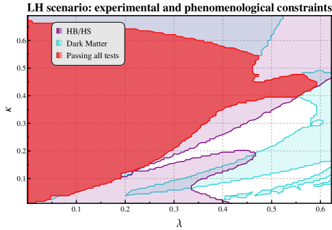
In Figure 3 we show the result of the scan in the NMSSM (λ,κ)𝜆𝜅(\lambda,\kappa)-plane after our tests. Light-blue-shaded area corresponds to points that pass DM constraints;666Here and in the following, we allow DM density to be below Planck [30] measured value. the points within purple-shaded boundary area pass the Higgs sector constraints from HiggsBounds and HiggsSignals. The solid red area is the region allowed by all the constraints, phenomenological and experimental ones, implemented within NMSSMTools, HiggsBounds and HiggsSignals.
Refer to caption
Figure 3: Light higgsino scenario: regions in the (λ,κ)𝜆𝜅(\lambda,\kappa)-plane allowed by experimental and phenomenological constraints. The light-blue-shaded regions delimited by the light blue boundary pass dark matter constraints. The coloured regions delimited by the purple boundary pass checks within HiggsBounds and HiggsSignals. The red area is allowed by all the constraints.

As a reference MSSM scenario, we select the one with M1subscript𝑀1M_{1}, M2subscript𝑀2M_{2}, μ=μeff𝜇subscript𝜇eff\mu=\mu_{\rm eff}, tanβ𝛽\tan\beta and the slepton masses given in Eqs. (5) and (6), to show that the light neutralino spectrum and production cross sections, see Table 7, may be very similar to the analogue quantities in the LH-NMSSM scenario in the vast part of the (λ,κ)𝜆𝜅(\lambda,\,\kappa)-plane, (cf. Figure 4 for mχ~10subscript𝑚subscriptsuperscript~𝜒01m_{\tilde{\chi}^{0}_{1}} and Figure 5 for the corresponding cross sections).

Regarding the Higgs sector, it is possible to get a MSSM counterpart with the same SM-Higgs mass and a similar spectrum for the other Higgs states (with the exception of the new singlet states) for each point in the (λ,κ)𝜆𝜅(\lambda,\,\kappa)-plane of the LH scenario.

mχ~10subscript𝑚subscriptsuperscript~𝜒01m_{\tilde{\chi}^{0}_{1}} mχ~20subscript𝑚subscriptsuperscript~𝜒02m_{\tilde{\chi}^{0}_{2}} mχ~30subscript𝑚subscriptsuperscript~𝜒03m_{\tilde{\chi}^{0}_{3}} mχ~40subscript𝑚subscriptsuperscript~𝜒04m_{\tilde{\chi}^{0}_{4}} mχ~1±subscript𝑚subscriptsuperscript~𝜒plus-or-minus1m_{\tilde{\chi}^{\pm}_{1}} mχ~2±subscript𝑚subscriptsuperscript~𝜒plus-or-minus2m_{\tilde{\chi}^{\pm}_{2}}
114.8 GeV 123.3 GeV 454.4 GeV 1604.1 GeV 119.4 GeV 1604.1 GeV
MSSM, σ(e+eχ~10χ~20)𝜎superscript𝑒superscript𝑒subscriptsuperscript~𝜒01subscriptsuperscript~𝜒02\sigma(e^{+}e^{-}\rightarrow\tilde{\chi}^{0}_{1}\tilde{\chi}^{0}_{2})\,\, s=350𝑠350\sqrt{s}=350 GeV s=500𝑠500\sqrt{s}=500 GeV
P=(0.9,0.55)𝑃0.90.55P=(-0.9,0.55) 791.7 fb 391.4 fb
P=(0.9,0.55)𝑃0.90.55P=(0.9,-0.55) 526.7 fb 261.7 fb
MSSM, σ(e+eχ~1+χ~1)𝜎superscript𝑒superscript𝑒subscriptsuperscript~𝜒1subscriptsuperscript~𝜒1\sigma(e^{+}e^{-}\rightarrow\tilde{\chi}^{+}_{1}\tilde{\chi}^{-}_{1}) s=350𝑠350\sqrt{s}=350 GeV s=500𝑠500\sqrt{s}=500 GeV
P=(0.9,0.55)𝑃0.90.55P=(-0.9,0.55) 2348.8 fb 1218.9 fb
P=(0.9,0.55)𝑃0.90.55P=(0.9,-0.55) 445.1 fb 246.2 fb
Table 7: The reference MSSM scenario for the LH scenario: neutralino and chargino masses [GeV] and production cross sections σ(e+eχ~10χ~20)𝜎superscript𝑒superscript𝑒subscriptsuperscript~𝜒01subscriptsuperscript~𝜒02\sigma(e^{+}e^{-}\rightarrow\tilde{\chi}^{0}_{1}\tilde{\chi}^{0}_{2}), σ(e+eχ~1+χ~1)𝜎superscript𝑒superscript𝑒subscriptsuperscript~𝜒1subscriptsuperscript~𝜒1\sigma(e^{+}e^{-}\rightarrow\tilde{\chi}^{+}_{1}\tilde{\chi}^{-}_{1}) [fb].

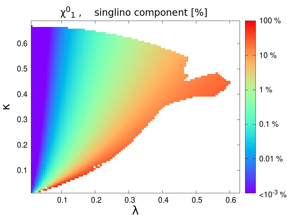
In Figure 4, the NMSSM χ~10subscriptsuperscript~𝜒01\tilde{\chi}^{0}_{1} mass and its singlino component are shown. A negligible singlino component corresponds to a region in which the NMSSM mχ~10subscript𝑚subscriptsuperscript~𝜒01m_{\tilde{\chi}^{0}_{1}} is very close to the MSSM value mχ~10=114.8subscript𝑚subscriptsuperscript~𝜒01114.8m_{\tilde{\chi}^{0}_{1}}=114.8 GeV. Vice versa, with a higher singlino admixture the LSP mass, mχ~10subscript𝑚subscriptsuperscript~𝜒01m_{\tilde{\chi}^{0}_{1}}, within NMSSM significantly decreases.
Refer to caption
Refer to caption
Figure 4: LH scenario: (a) the mass mχ~10subscript𝑚subscriptsuperscript~𝜒01m_{\tilde{\chi}^{0}_{1}}, in GeV; (b) the S~~𝑆\tilde{S} component of χ~10subscriptsuperscript~𝜒01\tilde{\chi}^{0}_{1}, in %.

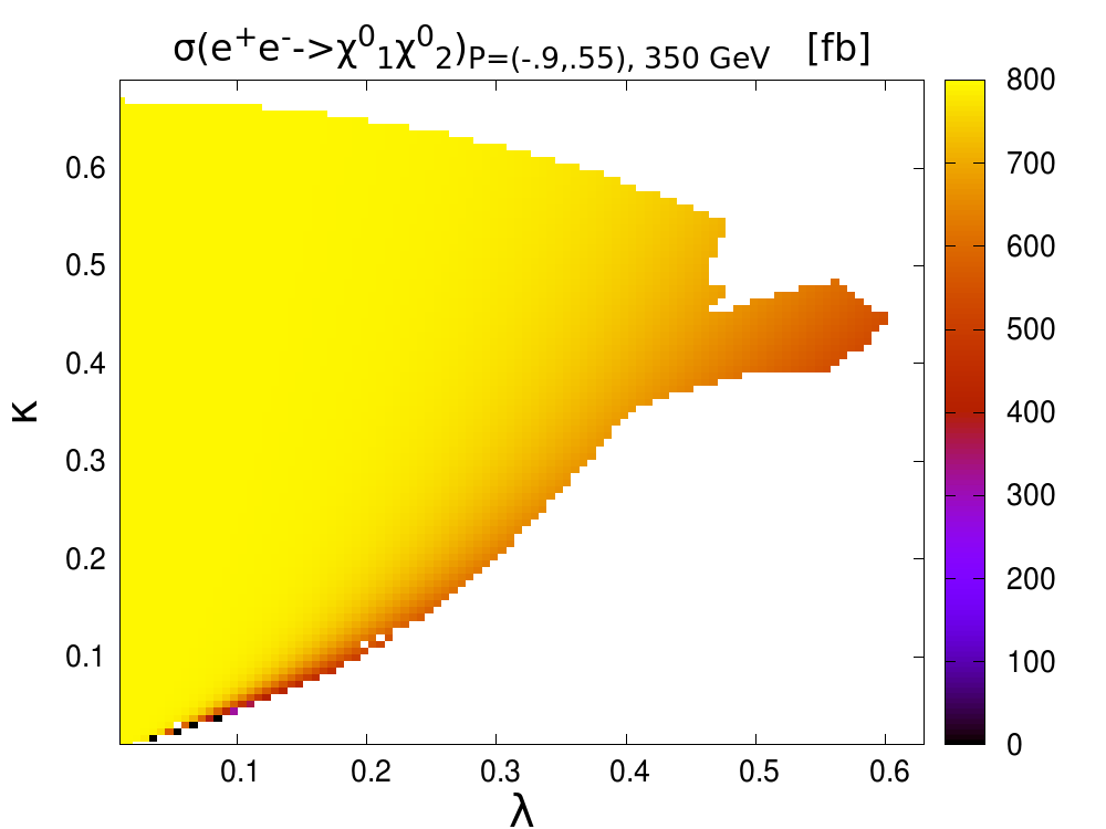
Likewise, the neutralino polarised production cross sections σ(e+eχ~10χ~20)𝜎superscript𝑒superscript𝑒subscriptsuperscript~𝜒01subscriptsuperscript~𝜒02\sigma(e^{+}e^{-}\rightarrow\tilde{\chi}^{0}_{1}\tilde{\chi}^{0}_{2}) decrease with respect to the MSSM value following larger singlino component in χ~10subscriptsuperscript~𝜒01\tilde{\chi}^{0}_{1}, see Figure 5, as it is expected since the singlino does not couple directly to the gauge fields. The tree-level NMSSM chargino masses and production cross-sections, σ(e+eχ~1+χ~1)𝜎superscript𝑒superscript𝑒subscriptsuperscript~𝜒1subscriptsuperscript~𝜒1\sigma(e^{+}e^{-}\rightarrow\tilde{\chi}^{+}_{1}\tilde{\chi}^{-}_{1}), depend only on M2subscript𝑀2M_{2}, μeffsubscript𝜇eff\mu_{\rm eff}, tanβ𝛽\tan\beta, therefore chargino production cross sections are identical to the MSSM values displayed in Table 7 along all the (λ,κ)𝜆𝜅(\lambda,\,\kappa)-plane.

Refer to caption
Refer to caption
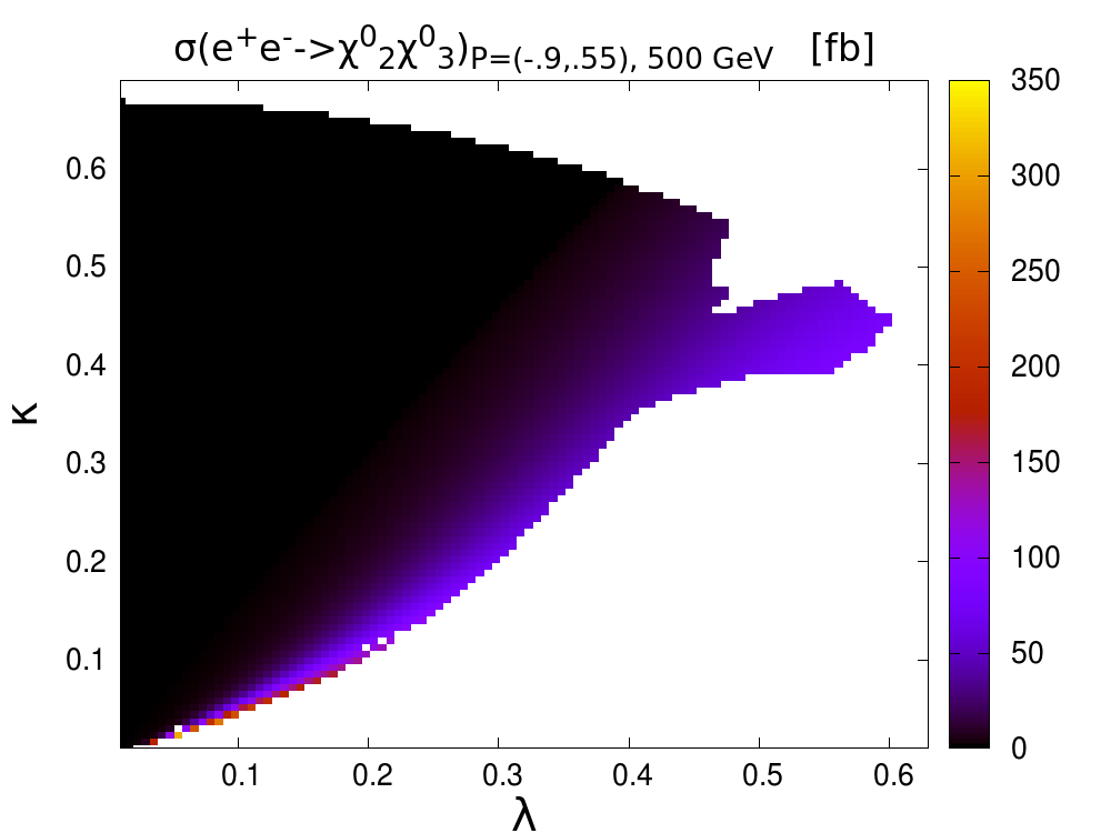
Figure 5: Production cross sections in the LH scenario: (a) σ(e+eχ~10χ~20)𝜎superscript𝑒superscript𝑒subscriptsuperscript~𝜒01subscriptsuperscript~𝜒02\sigma(e^{+}e^{-}\rightarrow\tilde{\chi}^{0}_{1}\tilde{\chi}^{0}_{2}) for P=(0.9,0.55)𝑃0.90.55P=(-0.9,0.55) at s=350𝑠350\sqrt{s}=350 GeV, in fb; (b) σ(e+eχ~20χ~30)𝜎superscript𝑒superscript𝑒subscriptsuperscript~𝜒02subscriptsuperscript~𝜒03\sigma(e^{+}e^{-}\rightarrow\tilde{\chi}^{0}_{2}\tilde{\chi}^{0}_{3}) for P=(0.9,+0.55)𝑃0.90.55P=(-0.9,+0.55) at s=500𝑠500\sqrt{s}=500 GeV, in fb.

According to the recipe in Section 2, we assume for each point in the (λ,κ)𝜆𝜅(\lambda,\,\kappa)-plane of the LH scenario the experimental measurement of:

  • mχ~10subscript𝑚subscriptsuperscript~𝜒01m_{\tilde{\chi}^{0}_{1}}, mχ~20subscript𝑚subscriptsuperscript~𝜒02m_{\tilde{\chi}^{0}_{2}} and mχ~1±subscript𝑚subscriptsuperscript~𝜒plus-or-minus1m_{\tilde{\chi}^{\pm}_{1}} with an uncertainty of 0.5%percent0.50.5\%.

  • σ(e+eχ~10χ~20)𝜎superscript𝑒superscript𝑒subscriptsuperscript~𝜒01subscriptsuperscript~𝜒02\sigma(e^{+}e^{-}\rightarrow\tilde{\chi}^{0}_{1}\tilde{\chi}^{0}_{2}) for P=(0.9,±0.55)𝑃minus-or-plus0.9plus-or-minus0.55P=(\mp 0.9,\pm 0.55) at s=350𝑠350\sqrt{s}=350 and 500 GeV with 1%percent11\% uncertainty.

  • σ(e+eχ~1+χ~1)𝜎superscript𝑒superscript𝑒subscriptsuperscript~𝜒1subscriptsuperscript~𝜒1\sigma(e^{+}e^{-}\rightarrow\tilde{\chi}^{+}_{1}\tilde{\chi}^{-}_{1}), for P=(0.9,±0.55)𝑃minus-or-plus0.9plus-or-minus0.55P=(\mp 0.9,\pm 0.55) at s=350𝑠350\sqrt{s}=350 and 500 GeV with 1%percent11\% uncertainty.

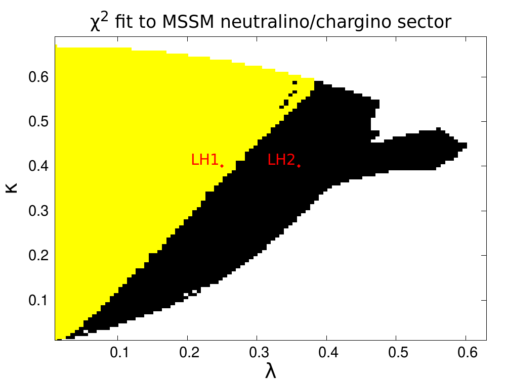
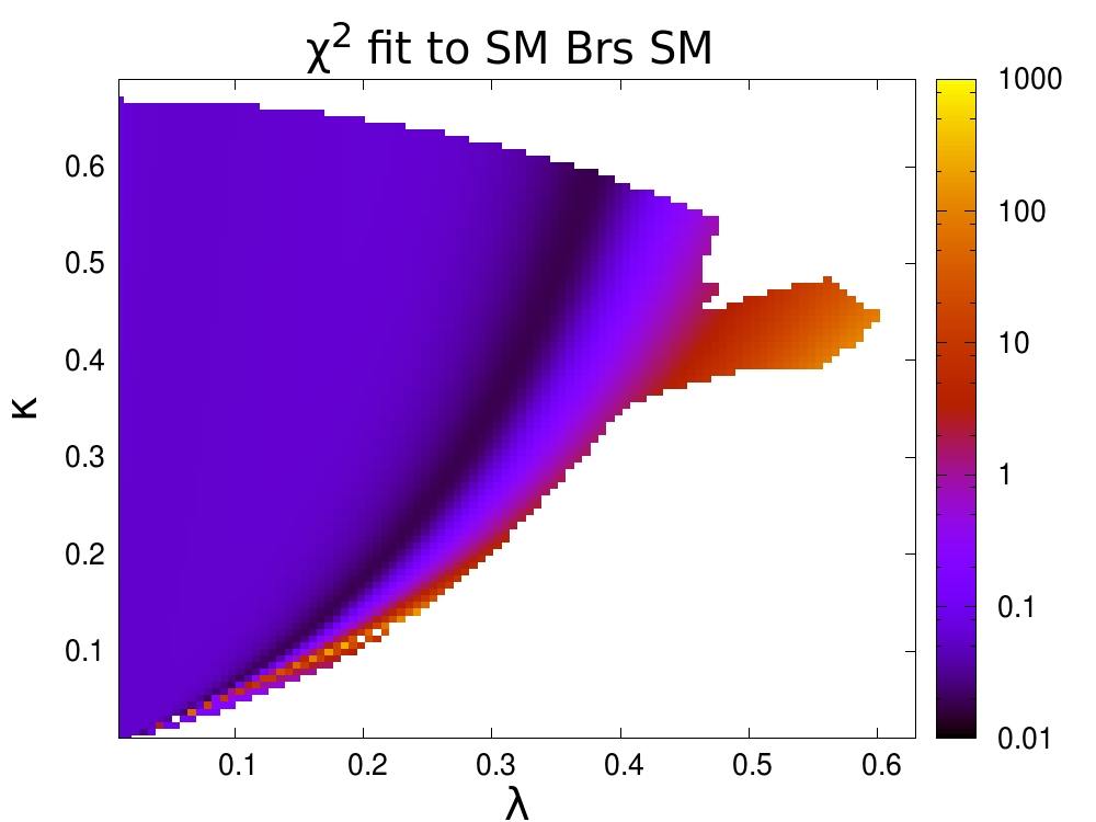
In the regions in which the singlino component in χ~30subscriptsuperscript~𝜒03\tilde{\chi}^{0}_{3} is higher, mχ~30subscript𝑚subscriptsuperscript~𝜒03m_{\tilde{\chi}^{0}_{3}} is decreased and χ~20χ~30subscriptsuperscript~𝜒02subscriptsuperscript~𝜒03\tilde{\chi}^{0}_{2}\tilde{\chi}^{0}_{3} may be kinematically accessible, see Figure 5. In these cases, if χ~30subscriptsuperscript~𝜒03\tilde{\chi}^{0}_{3} is detectable through its decays, we consider also mχ~30subscript𝑚subscriptsuperscript~𝜒03m_{\tilde{\chi}^{0}_{3}} and σ(e+eχ~20χ~30)𝜎superscript𝑒superscript𝑒subscriptsuperscript~𝜒02subscriptsuperscript~𝜒03\sigma(e^{+}e^{-}\rightarrow\tilde{\chi}^{0}_{2}\tilde{\chi}^{0}_{3}). The production χ~10χ~30subscriptsuperscript~𝜒01subscriptsuperscript~𝜒03\tilde{\chi}^{0}_{1}\tilde{\chi}^{0}_{3} is negligible almost everywhere. With these assumptions, a χ2superscript𝜒2\chi^{2}-fit to the MSSM gives the result displayed in Figure 6: the yellow areas correspond to regions in the (λ,κ)𝜆𝜅(\lambda,\,\kappa)-plane that are at 95% C.L. compatible with the MSSM, while in the black area MSSM is excluded. Therefore, a significant region of the parameter space, passing the implemented phenomenological and experimental constraints, can definitely be distinguished from the MSSM using collider observables. This is due to a higher singlino component in the neutralino χ~30subscriptsuperscript~𝜒03\tilde{\chi}^{0}_{3} (and partially in χ~10subscriptsuperscript~𝜒01\tilde{\chi}^{0}_{1} as well, cf. Figure 4.

Refer to caption
Figure 6: LH scenario: fit to the MSSM. Yellow areas are compatible with the MSSM at 95% C.L., while black ones are excluded by the collider observables. The points LH1 (λ,κ)=(0.25,0.4)𝜆𝜅0.250.4(\lambda,\kappa)=(0.25,0.4) and LH2 (λ,κ)=(0.36,0.4)𝜆𝜅0.360.4(\lambda,\kappa)=(0.36,0.4) are also shown.
Refer to caption
Refer to caption
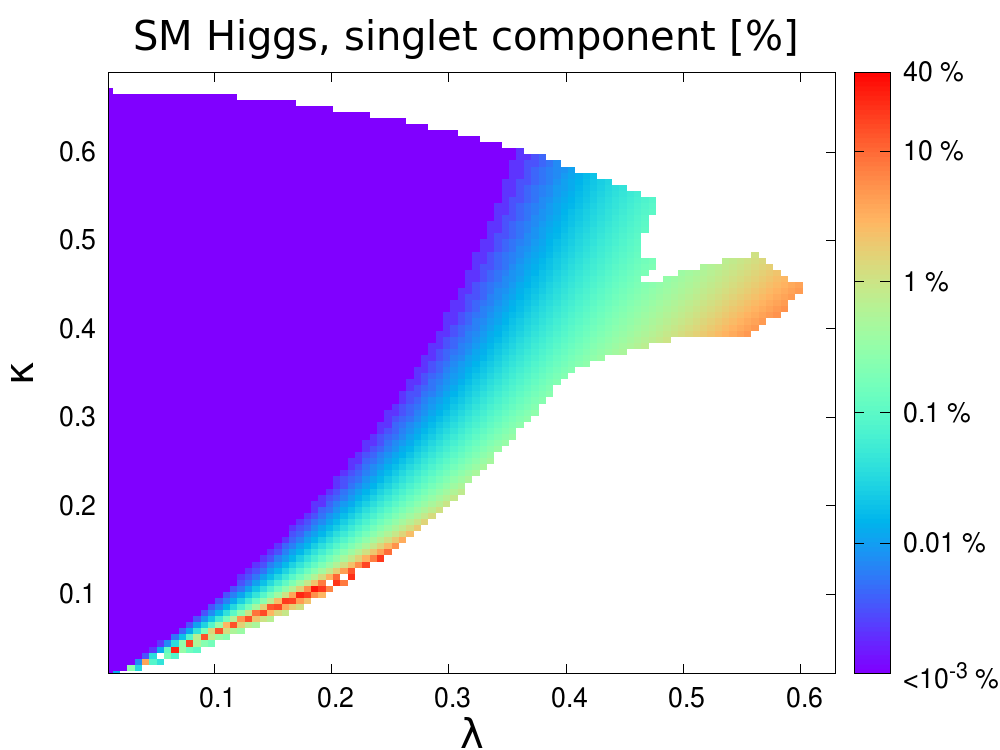
Figure 7: LH scenario: (a) 7-d.o.f. χ2superscript𝜒2\chi^{2}-fit to the SM of the reduced couplings to g,γ,W,Z,b,c,τ𝑔𝛾𝑊𝑍𝑏𝑐𝜏g,\gamma,W,Z,b,c,\tau; (b) Singlet component in the SM-like Higgs, in %.

We attempt here a reconstruction of the MSSM M1subscript𝑀1M_{1}, M2subscript𝑀2M_{2}, μ𝜇\mu, tanβ𝛽\tan\beta and mν~esubscript𝑚subscript~𝜈𝑒m_{\tilde{\nu}_{e}} for two sample points in the (λ,κ)𝜆𝜅(\lambda,\kappa)-plane of the LH scenario, relatively close to the boundary between the regions of compatibility from Figure 6.

  • The point LH1, with (λ,κ)=(0.25, 0.4)𝜆𝜅0.250.4(\lambda,\kappa)=(0.25,\,0.4), features the masses and cross sections given in Tables 8 and 9. The fit to LH1 turns out to be compatible with the MSSM, χ2=1.1superscript𝜒21.1\chi^{2}=1.1, and yields

    M1=360±40 GeV, M2=1300±300 GeV,subscript𝑀1plus-or-minus36040 GeV, subscript𝑀2plus-or-minus1300300 GeV,\displaystyle M_{1}=360\pm 40\mbox{ GeV,\,\,\, }\,\,M_{2}=1300\pm 300\mbox{ GeV, }
    μeff=124±2 GeV, tanβ4,subscript𝜇effplus-or-minus1242 GeV, 𝛽4\displaystyle\mu_{\rm eff}=124\pm 2\mbox{ GeV, }\,\,\,\tan\beta\leq 4,
    mν~e470GeV.subscript𝑚subscript~𝜈𝑒470GeV\displaystyle m_{\tilde{\nu}_{e}}\leq 470\;\mathrm{GeV}\,. (7)
  • For our second example, the point LH2 with (λ,κ)=(0.36, 0.4)𝜆𝜅0.360.4(\lambda,\kappa)=(0.36,\,0.4) is taken and the corresponding masses and cross sections are given in Tables 10 and 11. The point LH2 in not compatible with the MSSM, with the fit giving χ2=1700superscript𝜒21700\chi^{2}=1700 and the following parameter values:

    M1unconstrained,M2=317.0±0.5 GeV,subscript𝑀1unconstrainedsubscript𝑀2plus-or-minus317.00.5 GeV,\displaystyle M_{1}\;\;\mathrm{unconstrained,}\qquad\quad\;\,\,\,M_{2}=317.0\pm 0.5\mbox{ GeV, }
    μeff=129.3±0.6 GeV, tanβ<1.1,formulae-sequencesubscript𝜇effplus-or-minus129.30.6 GeV, 𝛽1.1\displaystyle\mu_{\rm eff}=129.3\pm 0.6\mbox{ GeV, }\quad\,\,\,\tan\beta<1.1,
    mν~e=297±15GeV.subscript𝑚subscript~𝜈𝑒plus-or-minus29715GeV\displaystyle m_{\tilde{\nu}_{e}}=297\pm 15\;\mathrm{GeV}. (8)
mχ~10subscript𝑚subscriptsuperscript~𝜒01m_{\tilde{\chi}^{0}_{1}} mχ~20subscript𝑚subscriptsuperscript~𝜒02m_{\tilde{\chi}^{0}_{2}} mχ~30subscript𝑚subscriptsuperscript~𝜒03m_{\tilde{\chi}^{0}_{3}} mχ~40subscript𝑚subscriptsuperscript~𝜒04m_{\tilde{\chi}^{0}_{4}} mχ~50subscript𝑚subscriptsuperscript~𝜒05m_{\tilde{\chi}^{0}_{5}} mχ~1±subscript𝑚subscriptsuperscript~𝜒plus-or-minus1m_{\tilde{\chi}^{\pm}_{1}} mχ~2±subscript𝑚subscriptsuperscript~𝜒plus-or-minus2m_{\tilde{\chi}^{\pm}_{2}}
111.6 GeV 125.2 GeV 389.0 GeV 454.4 GeV 1604 GeV 119.4 GeV 1604 GeV
Table 8: Neutralino and chargino masses in the light higgsino scenario for the reference point LH1 with (λ,κ)=𝜆𝜅absent(\lambda,\kappa)=(0.25, 0.4).
σ(e+eχ~10χ~20)𝜎superscript𝑒superscript𝑒subscriptsuperscript~𝜒01subscriptsuperscript~𝜒02\sigma(e^{+}e^{-}\rightarrow\tilde{\chi}^{0}_{1}\tilde{\chi}^{0}_{2}) s=350𝑠350\sqrt{s}=350 GeV s=500𝑠500\sqrt{s}=500 GeV
P=(0.9,0.55)𝑃0.90.55P=(-0.9,0.55) 781.5 fb 385.8 fb
P=(0.9,0.55)𝑃0.90.55P=(0.9,-0.55) 519.9 fb 257.9 fb
Table 9: Neutralino production cross sections in the light higgsino scenario, reference point LH1 with (λ,κ)=𝜆𝜅absent(\lambda,\kappa)=(0.25, 0.4).
mχ~10subscript𝑚subscriptsuperscript~𝜒01m_{\tilde{\chi}^{0}_{1}} mχ~20subscript𝑚subscriptsuperscript~𝜒02m_{\tilde{\chi}^{0}_{2}} mχ~30subscript𝑚subscriptsuperscript~𝜒03m_{\tilde{\chi}^{0}_{3}} mχ~40subscript𝑚subscriptsuperscript~𝜒04m_{\tilde{\chi}^{0}_{4}} mχ~50subscript𝑚subscriptsuperscript~𝜒05m_{\tilde{\chi}^{0}_{5}} mχ~1±subscript𝑚subscriptsuperscript~𝜒plus-or-minus1m_{\tilde{\chi}^{\pm}_{1}} mχ~2±subscript𝑚subscriptsuperscript~𝜒plus-or-minus2m_{\tilde{\chi}^{\pm}_{2}}
104.2 GeV 128.4 GeV 282.4 GeV 454.4 GeV 1604 GeV 119.4 GeV 1604 GeV
Table 10: Neutralino and chargino masses in the light higgsino scenario for the reference point LH2 with (λ,κ)=𝜆𝜅absent(\lambda,\kappa)=(0.36, 0.4).
σ(e+eχ~10χ~20)𝜎superscript𝑒superscript𝑒subscriptsuperscript~𝜒01subscriptsuperscript~𝜒02\sigma(e^{+}e^{-}\rightarrow\tilde{\chi}^{0}_{1}\tilde{\chi}^{0}_{2}) s=350𝑠350\sqrt{s}=350 GeV s=500𝑠500\sqrt{s}=500 GeV
P=(0.9,0.55)𝑃0.90.55P=(-0.9,0.55) 739.0 fb 363.3 fb
P=(0.9,0.55)𝑃0.90.55P=(0.9,-0.55) 491.5 fb 242.8 fb
σ(e+eχ~20χ~30)𝜎superscript𝑒superscript𝑒subscriptsuperscript~𝜒02subscriptsuperscript~𝜒03\sigma(e^{+}e^{-}\rightarrow\tilde{\chi}^{0}_{2}\tilde{\chi}^{0}_{3}) s=350𝑠350\sqrt{s}=350 GeV s=500𝑠500\sqrt{s}=500 GeV
P=(0.9,0.55)𝑃0.90.55P=(-0.9,0.55) not accessible 15.4 fb
P=(0.9,0.55)𝑃0.90.55P=(0.9,-0.55) not accessible 10.4 fb
Table 11: Neutralino production cross sections in the light higgsino scenario for the reference point LH2 with (λ,κ)=𝜆𝜅absent(\lambda,\kappa)=(0.36, 0.4).

Additional information from the heavier neutralino states, such as χ~30subscriptsuperscript~𝜒03\tilde{\chi}^{0}_{3} (if its production is not already kinematically allowed at 500 GeV) or χ~40subscriptsuperscript~𝜒04\tilde{\chi}^{0}_{4}, may help in reducing the region compatible with the MSSM. For example, given a (λ,κ)𝜆𝜅(\lambda,\kappa) coordinate and the corresponding M1subscript𝑀1M_{1}, M2subscript𝑀2M_{2}, μ𝜇\mu, tanβ𝛽\tan\beta reconstructed from the fit, one can derive the masses of the heavier states and look for them at higher energies at the ILC or at the LHC, either confirming the fit to the MSSM or pinpointing the NMSSM.

As suggested in Section 2, our study may be extended by including information from the Higgs sector. A result of the naïve χ2superscript𝜒2\chi^{2}-fit to the SM of the Higgs reduced couplings to g,γ,W,Z,b,c,τ𝑔𝛾𝑊𝑍𝑏𝑐𝜏g,\gamma,W,Z,b,c,\tau, each defined as a ratio gh/ghSMsubscript𝑔subscript𝑔subscriptSMg_{h}/g_{h_{\rm SM}} between the SM-like Higgs coupling to the corresponding SM Higgs coupling, is shown in Figure 7.777We used the expected accuracies for the SM-like Higgs boson branching ratios ΔBr/BrΔBrBr\Delta\mbox{Br}/\mbox{Br} from [34]. In large part of the (λ,κ)𝜆𝜅(\lambda,\kappa)-plane, the SM-like Higgs of the LH scenario is compatible with the SM (χ214less-than-or-similar-tosuperscript𝜒214\chi^{2}\lesssim 14), corresponding to the MSSM-like area from the fit in Figure 6. A SM-like Higgs with a higher singlet component, see Figure 7, corresponds to a worse fit: there are two regions that are not compatible with the SM and have a different behaviour with respect of MSSM-like areas. The conclusion from this fit is therefore consistent with that of Figure 6 without clearly improving our analysis.

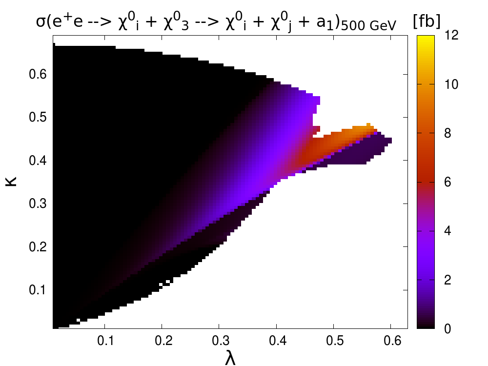
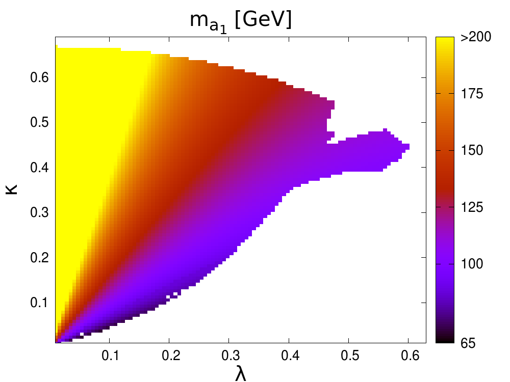
Additional information about the NMSSM Higgs sector could obtained if new singlets are directly visible. This possibility opens up in a region with a higher singlino component in χ~30subscriptsuperscript~𝜒03\tilde{\chi}^{0}_{3}, where the decays χ~30χ~1,20a1subscriptsuperscript~𝜒03subscriptsuperscript~𝜒012subscript𝑎1\tilde{\chi}^{0}_{3}\rightarrow\tilde{\chi}^{0}_{1,2}a_{1} become open. If the production cross section for χ~30subscriptsuperscript~𝜒03\tilde{\chi}^{0}_{3} is non-negligible one could observe the pseudoscalar a1subscript𝑎1a_{1} via its decays a1bb¯subscript𝑎1𝑏¯𝑏a_{1}\to b\bar{b}. In Figure 8 we show an inclusive cross section for production of a1subscript𝑎1a_{1}, where both production modes, e+eχ~10χ~30superscript𝑒superscript𝑒subscriptsuperscript~𝜒01subscriptsuperscript~𝜒03e^{+}e^{-}\to\tilde{\chi}^{0}_{1}\tilde{\chi}^{0}_{3} and e+eχ~20χ~30superscript𝑒superscript𝑒subscriptsuperscript~𝜒02subscriptsuperscript~𝜒03e^{+}e^{-}\to\tilde{\chi}^{0}_{2}\tilde{\chi}^{0}_{3}, for both polarisations has been added up together with decays χ~30χ~10a1subscriptsuperscript~𝜒03subscriptsuperscript~𝜒01subscript𝑎1\tilde{\chi}^{0}_{3}\to\tilde{\chi}^{0}_{1}a_{1} and χ~30χ~20a1subscriptsuperscript~𝜒03subscriptsuperscript~𝜒02subscript𝑎1\tilde{\chi}^{0}_{3}\to\tilde{\chi}^{0}_{2}a_{1}. In certain regions of parameter space, with cross sections of order 10 fb, the new state should be clearly visible. This could serve as confirmation of the NMSSM, since the MSSM would be already excluded by the fit to other observables. As a reference, in Figure 8 we also show the mass of the pseudoscalar a1subscript𝑎1a_{1}.

Refer to caption
Refer to caption
Figure 8: LH scenario: (a) inclusive cross section e+eχ~i0χ~30χ~i0χ~j0a1superscript𝑒superscript𝑒subscriptsuperscript~𝜒0𝑖subscriptsuperscript~𝜒03subscriptsuperscript~𝜒0𝑖subscriptsuperscript~𝜒0𝑗subscript𝑎1e^{+}e^{-}\rightarrow\tilde{\chi}^{0}_{i}\tilde{\chi}^{0}_{3}\rightarrow\tilde{\chi}^{0}_{i}\tilde{\chi}^{0}_{j}a_{1} [fb], with i,j=1,2formulae-sequence𝑖𝑗12i,\,j=1,2; (b) lightest CP-odd Higgs mass ma1subscript𝑚subscript𝑎1m_{a_{1}} [GeV].

3.3 Light gaugino scenario, μeff>M1>M2subscript𝜇effsubscript𝑀1subscript𝑀2\mu_{\rm eff}>M_{1}>M_{2}

Finally, we study an NMSSM scenario with light gauginos (LG), whose neutralino/chargino sector is given by:

M1=240 GeV, M2=105 GeV, μ=μeff=505 GeV, tanβ=9.2,subscript𝑀1240 GeV, subscript𝑀2105 GeV, 𝜇subscript𝜇eff505 GeV, 𝛽9.2M_{1}=240\mbox{ GeV,\,\,\, }\,\,\,M_{2}=105\mbox{ GeV, }\,\,\,\mu=\mu_{\rm eff}=505\mbox{ GeV, }\,\,\,\tan\beta=9.2\,, (9)

with λ[0,0.7]𝜆00.7\lambda\in[0,0.7] and κ[0,0.7]𝜅00.7\kappa\in[0,0.7]. The singlet soft trilinear parameters are Aλ=3700subscript𝐴𝜆3700A_{\lambda}=3700 GeV, Aκ=40subscript𝐴𝜅40A_{\kappa}=-40 GeV. The first generation sfermion masses are

me~L=303.4 GeV,me~L=me~R,mν~e2=me~L2+cos(2β)cos2θWmZ2,formulae-sequencesubscript𝑚subscript~𝑒𝐿303.4 GeVformulae-sequencesubscript𝑚subscript~𝑒𝐿subscript𝑚subscript~𝑒𝑅superscriptsubscript𝑚subscript~𝜈𝑒2superscriptsubscript𝑚subscript~𝑒𝐿22𝛽superscript2subscript𝜃𝑊superscriptsubscript𝑚𝑍2m_{\tilde{e}_{L}}=303.4\mbox{ GeV},\,\,\,m_{\tilde{e}_{L}}=m_{\tilde{e}_{R}},\,\,\,m_{\tilde{\nu}_{e}}^{2}=m_{\tilde{e}_{L}}^{2}+\cos(2\beta)\cos^{2}\theta_{W}m_{Z}^{2}, (10)

while squarks masses are >1absent1>1 TeV. For the full set of soft parameters, we refer to Appendix B.3.

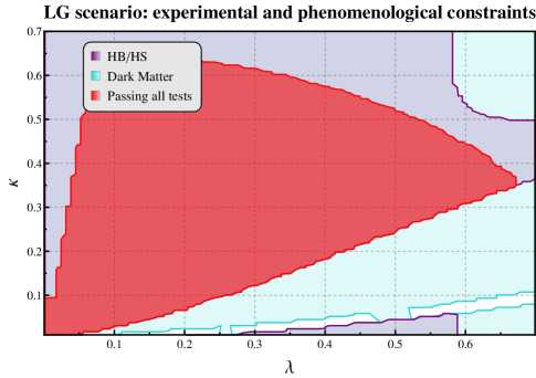
In Figure 9 we display the result of the scan in the NMSSM (λ,κ)𝜆𝜅(\lambda,\kappa)-plane after our tests implemented within NMSSMTools, HiggsBounds and HiggsSignals. The colour conventions are the same as for the LH scenario, Section 3.2; for the LG scenario the regions allowed by the Higgs sector constraints from HiggsBounds and HiggsSignals overlap entirely those passing DM matter constraints.
Refer to caption
Figure 9: The light gaugino scenario: regions in the (λ,κ)𝜆𝜅(\lambda,\kappa)-plane allowed by experimental and phenomenological constraints. The light-blue region passes the dark matter constraints. The purple-coloured region passes checks from HiggsBounds and HiggsSignals. The areas allowed by all the constraints are shown in red.

A reference MSSM scenario with an almost indistinguishable lighter (tree-level) neutralino and chargino mass spectrum and production cross sections is found by choosing M1subscript𝑀1M_{1}, M2subscript𝑀2M_{2}, μ𝜇\mu, tanβ𝛽\tan\beta and the first generation slepton masses as in Eq. (9), see Table 12.

mχ~10subscript𝑚subscriptsuperscript~𝜒01m_{\tilde{\chi}^{0}_{1}} mχ~20subscript𝑚subscriptsuperscript~𝜒02m_{\tilde{\chi}^{0}_{2}} mχ~30subscript𝑚subscriptsuperscript~𝜒03m_{\tilde{\chi}^{0}_{3}} mχ~40subscript𝑚subscriptsuperscript~𝜒04m_{\tilde{\chi}^{0}_{4}} mχ~1±subscript𝑚subscriptsuperscript~𝜒plus-or-minus1m_{\tilde{\chi}^{\pm}_{1}} mχ~2±subscript𝑚subscriptsuperscript~𝜒plus-or-minus2m_{\tilde{\chi}^{\pm}_{2}}
99.5 GeV 237.0 GeV 510.1 GeV 518.7 GeV 99.6 GeV 518.7 GeV
MSSM, σ(e+eχ~10χ~20)𝜎superscript𝑒superscript𝑒subscriptsuperscript~𝜒01subscriptsuperscript~𝜒02\sigma(e^{+}e^{-}\rightarrow\tilde{\chi}^{0}_{1}\tilde{\chi}^{0}_{2}) s=350𝑠350\sqrt{s}=350 GeV s=500𝑠500\sqrt{s}=500 GeV
P=(0.9,0.55)𝑃0.90.55P=(-0.9,0.55) 7.3 fb 113.4 fb
P=(0.9,0.55)𝑃0.90.55P=(0.9,-0.55) 0.1 fb 1.8 fb
MSSM, σ(e+eχ~1+χ~1)𝜎superscript𝑒superscript𝑒subscriptsuperscript~𝜒1subscriptsuperscript~𝜒1\sigma(e^{+}e^{-}\rightarrow\tilde{\chi}^{+}_{1}\tilde{\chi}^{-}_{1}) s=350𝑠350\sqrt{s}=350 GeV s=500𝑠500\sqrt{s}=500 GeV
P=(0.9,0.55)𝑃0.90.55P=(-0.9,0.55) 2692.1 fb 1252.6 fb
P=(0.9,0.55)𝑃0.90.55P=(0.9,-0.55) 44.5 fb 19.4 fb
Table 12: The reference light gaugino MSSM scenario: neutralino and chargino masses [GeV] and production cross sections σ(e+eχ~10χ~20)𝜎superscript𝑒superscript𝑒subscriptsuperscript~𝜒01subscriptsuperscript~𝜒02\sigma(e^{+}e^{-}\rightarrow\tilde{\chi}^{0}_{1}\tilde{\chi}^{0}_{2}), σ(e+eχ~1+χ~1)𝜎superscript𝑒superscript𝑒subscriptsuperscript~𝜒1subscriptsuperscript~𝜒1\sigma(e^{+}e^{-}\rightarrow\tilde{\chi}^{+}_{1}\tilde{\chi}^{-}_{1}) [fb].
Refer to caption
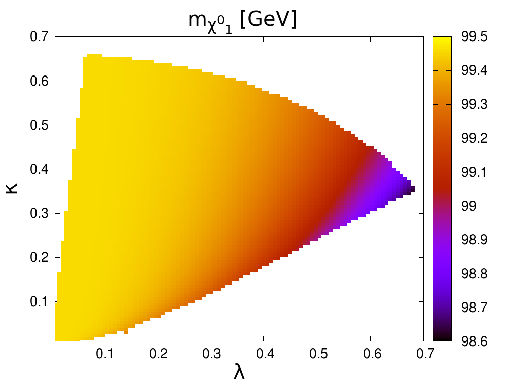
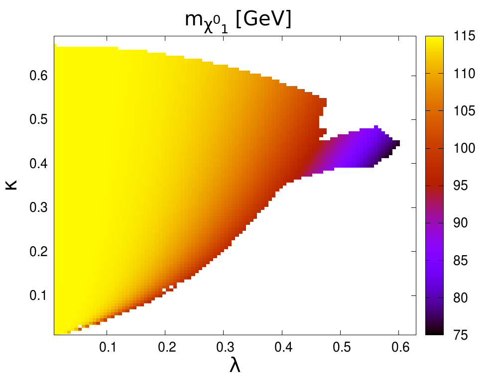
Figure 10: The LG scenario: the mass mχ~10subscript𝑚subscriptsuperscript~𝜒01m_{\tilde{\chi}^{0}_{1}} [GeV].

In the LG scenario mχ~10subscript𝑚subscriptsuperscript~𝜒01m_{\tilde{\chi}^{0}_{1}} is very close to the reference MSSM value 99.5 GeV and it varies very mildly in the (λ,κ)𝜆𝜅(\lambda,\,\kappa)-plane as the singlino component in χ~10subscriptsuperscript~𝜒01\tilde{\chi}^{0}_{1} is approximately zero, see Figure 10. A similar reasoning applies to the production cross section σ(e+eχ~10χ~20)𝜎superscript𝑒superscript𝑒subscriptsuperscript~𝜒01subscriptsuperscript~𝜒02\sigma(e^{+}e^{-}\rightarrow\tilde{\chi}^{0}_{1}\tilde{\chi}^{0}_{2}), while the chargino production, σ(e+eχ~1+χ~1)𝜎superscript𝑒superscript𝑒subscriptsuperscript~𝜒1subscriptsuperscript~𝜒1\sigma(e^{+}e^{-}\rightarrow\tilde{\chi}^{+}_{1}\tilde{\chi}^{-}_{1}), is exactly identical at the tree-level as explained in Section 3.2.

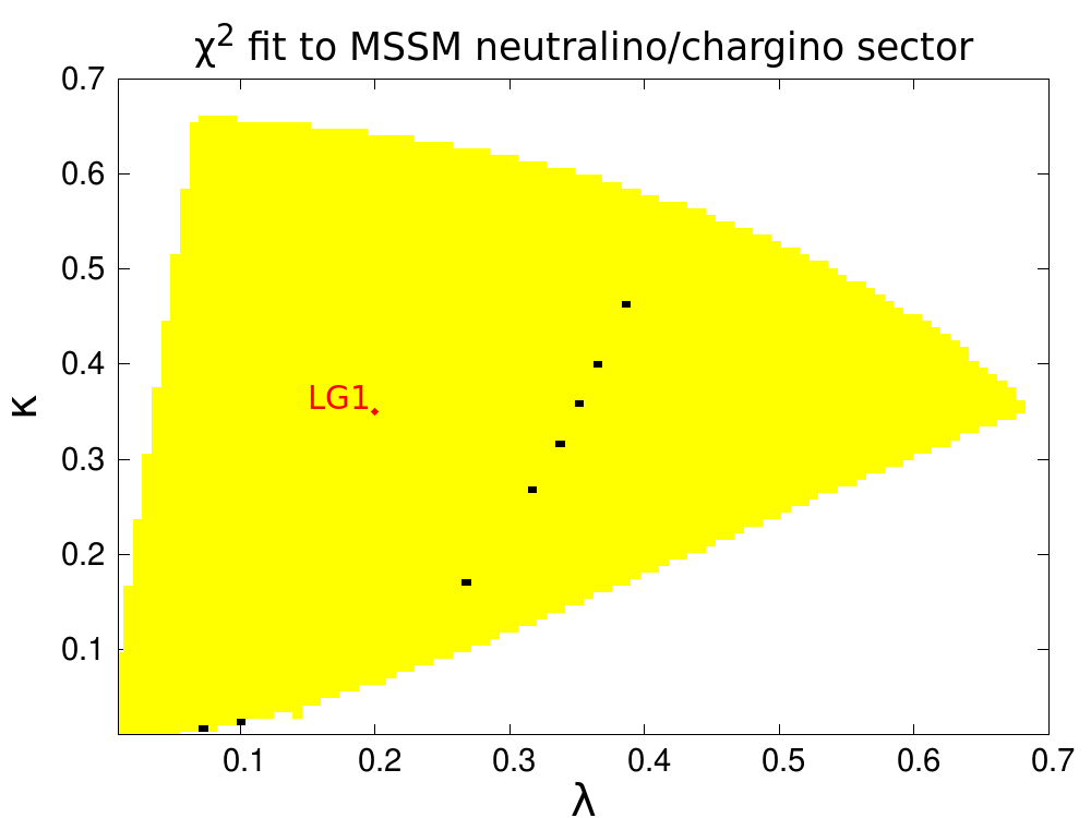
We only use cross sections larger than 1 fb for χ2superscript𝜒2\chi^{2}-fit to the MSSM. Figure 11 shows that our fit alone is not able to distinguish in this case between the two models, as basically every point in the allowed region is compatible with the MSSM.

As example we analyse the point LG1 with (λ,κ)=(0.2,0.35)𝜆𝜅0.20.35(\lambda,\kappa)=(0.2,0.35) and the remaining parameters given by Eqs. (9) and (10) that features the masses and cross sections listed in Tables 13 and 14. For P=(0.9,0.55)𝑃0.90.55P=(0.9,-0.55) the cross section σ(e+eχ~10χ~20)𝜎superscript𝑒superscript𝑒subscriptsuperscript~𝜒01subscriptsuperscript~𝜒02\sigma(e^{+}e^{-}\rightarrow\tilde{\chi}^{0}_{1}\tilde{\chi}^{0}_{2}) at s=350𝑠350\sqrt{s}=350 GeV is below 1 fb and the process e+eχ~10χ~30superscript𝑒superscript𝑒subscriptsuperscript~𝜒01subscriptsuperscript~𝜒03e^{+}e^{-}\rightarrow\tilde{\chi}^{0}_{1}\tilde{\chi}^{0}_{3} is kinematically not allowed for both at 350 and 500 GeV. The remaining observables lead to a fit that is compatible with the MSSM giving χ2superscript𝜒2\chi^{2}=0.07:

M1=239.9±0.9 GeV, M2=104.4±0.8 GeV,subscript𝑀1plus-or-minus239.90.9 GeV, subscript𝑀2plus-or-minus104.40.8 GeV,\displaystyle M_{1}=239.9\pm 0.9\mbox{ GeV,\,\,\, }\,\,M_{2}=104.4\pm 0.8\mbox{ GeV, }
μeff=504.7±47.6 GeV, tanβ=11.4±2.8,subscript𝜇effplus-or-minus504.747.6 GeV, 𝛽plus-or-minus11.42.8\displaystyle\mu_{\rm eff}=504.7\pm 47.6\mbox{ GeV, }\,\,\,\tan\beta=11.4\pm 2.8,
mν~e=292.8±3.9GeV.subscript𝑚subscript~𝜈𝑒plus-or-minus292.83.9GeV\displaystyle m_{\tilde{\nu}_{e}}=292.8\pm 3.9\;\mathrm{GeV}\,. (11)

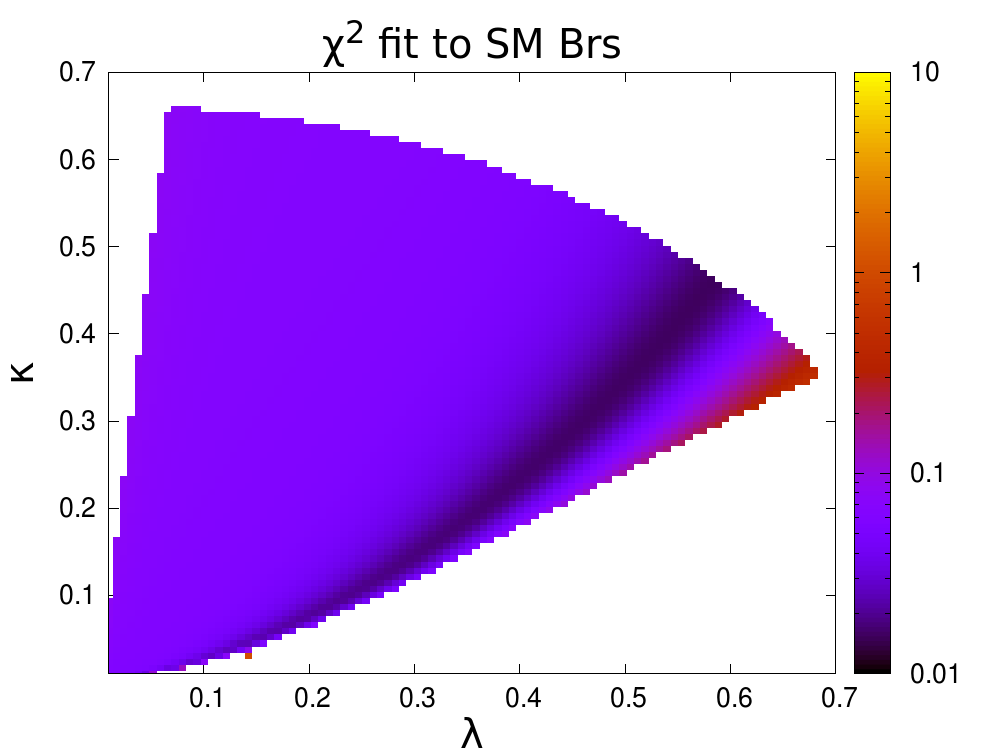
These values are remarkably close to the ‘true’ input parameters given by Eqs. (9) and (10). A naïve fit of the SM-like Higgs reduced couplings does not provide information useful for model distinction, see Figure 11, as they are always compatible with the SM, unlike in the LH scenario.

mχ~10subscript𝑚subscriptsuperscript~𝜒01m_{\tilde{\chi}^{0}_{1}} mχ~20subscript𝑚subscriptsuperscript~𝜒02m_{\tilde{\chi}^{0}_{2}} mχ~30subscript𝑚subscriptsuperscript~𝜒03m_{\tilde{\chi}^{0}_{3}} mχ~40subscript𝑚subscriptsuperscript~𝜒04m_{\tilde{\chi}^{0}_{4}} mχ~50subscript𝑚subscriptsuperscript~𝜒05m_{\tilde{\chi}^{0}_{5}} mχ~1±subscript𝑚subscriptsuperscript~𝜒plus-or-minus1m_{\tilde{\chi}^{\pm}_{1}} mχ~2±subscript𝑚subscriptsuperscript~𝜒plus-or-minus2m_{\tilde{\chi}^{\pm}_{2}}
99.4 GeV 237.0 GeV 510.4 GeV 518.3 GeV 1768.2 GeV 99.5 GeV 518.7 GeV
Table 13: Neutralino and chargino masses in the light gaugino scenario for the reference point LG1 with (λ,κ)=𝜆𝜅absent(\lambda,\kappa)=(0.2, 0.35).
σ(e+eχ~10χ~20)𝜎superscript𝑒superscript𝑒subscriptsuperscript~𝜒01subscriptsuperscript~𝜒02\sigma(e^{+}e^{-}\rightarrow\tilde{\chi}^{0}_{1}\tilde{\chi}^{0}_{2}) s=350𝑠350\sqrt{s}=350 GeV s=500𝑠500\sqrt{s}=500 GeV
P=(0.9,0.55)𝑃0.90.55P=(-0.9,0.55) 7.3 fb 113.5 fb
P=(0.9,0.55)𝑃0.90.55P=(0.9,-0.55) 0.1 fb 1.8 fb
Table 14: Neutralino production cross sections in the light gaugino scenario for the reference point LG1 with (λ,κ)=𝜆𝜅absent(\lambda,\kappa)=(0.2, 0.35).
Refer to caption
Refer to caption
Figure 11: LG scenario: (a) fit to the MSSM. Yellow areas are compatible with the MSSM at 95% C.L., while black ones are excluded by the collider observables. The point LG1 (λ,κ)=𝜆𝜅absent(\lambda,\kappa)=(0.2, 0.35) is displayed. (b) χ2superscript𝜒2\chi^{2}-fit to the SM of the reduced Higgs boson couplings to g,γ,W,Z,b,c,τ𝑔𝛾𝑊𝑍𝑏𝑐𝜏g,\gamma,W,Z,b,c,\tau.

This behaviour can be understood by analysing the mixing within the neutralino sector. In the NMSSM, the singlino does not mix directly with gauginos but only indirectly via higgsino states, see Eq. (18) and Appendix A.1. If, like in the LG scenario, μeffM1,M2much-greater-thansubscript𝜇effsubscript𝑀1subscript𝑀2\mu_{\rm eff}\gg M_{1},M_{2}, the mixing remains small even for a relatively light singlino. Therefore the properties of the light chargino and neutralino states, including masses and cross sections, remain very similar throughout the (λ,κ)𝜆𝜅(\lambda,\kappa)-plane and cannot be distinguished from the MSSM case. In contrast to that, in the light singlino scenario from Section 3.1, M1=365subscript𝑀1365M_{1}=365 GeV and μeff=484subscript𝜇eff484\mu_{\rm eff}=484 GeV are of the similar size resulting in significant mixing: χ~2022%B~+73%S~similar-to-or-equalssubscriptsuperscript~𝜒02percent22~𝐵percent73~𝑆\tilde{\chi}^{0}_{2}\simeq 22\%\,\tilde{B}+73\%\,\tilde{S} and χ~3072%B~+25%S~similar-to-or-equalssubscriptsuperscript~𝜒03percent72~𝐵percent25~𝑆\tilde{\chi}^{0}_{3}\simeq 72\%\,\tilde{B}+25\%\,\tilde{S}. Since in the LS case the singlino component makes up a significant part of the light neutralinos, the modification of the couplings allows the clear discrimination from the MSSM.

4 Conclusions and outlook

It will be very important to develop methods how to discriminate between the NMSSM and the MSSM at future experiments, as the two models may reproduce experimentally very similar light Higgs sectors as well as lower supersymmetric spectra. In this paper we have outlined a model distinction strategy that focuses on the neutralino and chargino sector and we have applied it to a series of NMSSM scenarios with different singlino, gaugino and higgsino properties. The idea is to assume that the lightest neutralino and chargino masses as well as their polarised pair production cross sections are measurable at a linear collider and to reconstruct the corresponding MSSM parameters, M1,M2,μ,tanβsubscript𝑀1subscript𝑀2𝜇𝛽M_{1},\,M_{2},\,\mu,\tan\beta, via a χ2superscript𝜒2\chi^{2}-fit. In case such a fit clearly excludes the MSSM hypothesis it would strongly point towards an extended model, preferably the NMSSM. Integrating the analysis with further information from the Higgs sector or from heavier neutralino resonances could confirm such a new model hypothesis. Throughout our study we have assumed to operate at the ILC with two different energy stages, namely at s=350𝑠350\sqrt{s}=350 and 500 GeV, using electron and positron beam polarisation with P=(±0.9,0.55)𝑃plus-or-minus0.9minus-or-plus0.55P=(\pm 0.9,\mp 0.55).

We have introduced three classes of scenarios with different phenomenological aspects concerning the model distinction: a light singlino, a light higgsino and a light gaugino scenario. We have first analysed an NMSSM scenario with singlino components in the χ~20subscriptsuperscript~𝜒02\tilde{\chi}^{0}_{2} and a wino-like LSP χ~10subscriptsuperscript~𝜒01\tilde{\chi}^{0}_{1}, i.e. with an inverted hierarchy of the gaugino mass parameters. Such a NMSSM scenario does not result in set of observables consistent with the MSSM. Accessing the mixing character of the heavier neutralino χ~30subscriptsuperscript~𝜒03\tilde{\chi}^{0}_{3} would confirm the situation and point to a model with an extended neutralino sector with respect to the MSSM.

In the class with light higgsinos, one usually has the hierarchy μeff<M1<M2subscript𝜇effsubscript𝑀1subscript𝑀2\mu_{\rm eff}<M_{1}<M_{2}. In the corresponding NMSSM parameter space, a large part of the (λ,κ)𝜆𝜅(\lambda,\kappa)-plane features the heavy and decoupled singlino while the χ~10subscriptsuperscript~𝜒01\tilde{\chi}^{0}_{1} is higgsino-like. Such a model is indistinguishable from the MSSM. However, if a sufficient singlino admixture is present in the light neutralinos, the neutralino sector changes appreciably, allowing for a discrimination between the MSSM and the NMSSM. In some region of the parameter space additional pseudoscalar Higgs a1subscript𝑎1a_{1} could also be observed. Precise measurement of the SM-like Higgs couplings would be beneficial for a confirmation of these conclusions.

As a third class we have chosen light gaugino scenarios again with an inverted hierarchy M2<M1<μeffsubscript𝑀2subscript𝑀1subscript𝜇effM_{2}<M_{1}<\mu_{\rm eff} but with μeffM1𝒪(250)similar-tosubscript𝜇effsubscript𝑀1𝒪250\mu_{\rm eff}-M_{1}\sim\mathcal{O}(250) GeV. In this way the singlino does not significantly mix with gauginos in the lightest neutralino states. In the light of our experimental assumptions, the low mass spectrum and production cross sections are not distinguishable from the MSSM ones all over the allowed (λ,κ)𝜆𝜅(\lambda,\kappa)-plane. In this case analysing the SM-like Higgs couplings also does not provide further information.

Our studies show that the neutralino and chargino sector can provide the crucial information for the model distinction between the MSSM and the NMSSM. Such a discrimination depends on the gaugino mass hierarchies and the actual singlino admixture in the light neutralino states. Precise measurements and a model-independent analysis for the determination of the fundamental SUSY parameters are essential.

Acknowledgements

The authors are thankful to M. Berggren, F. Domingo, P. Gunnellini, J. List, O. Stål, M. Tonini, M. de Vries, G. Weiglein and L. Zeune for useful discussions. S. P. has been supported by DFG through the grant SFB 676 “Particles, Strings, and the Early Universe”. This work has been partially supported by the MICINN, Spain, under contract FPA2010-17747; Consolider-Ingenio CPAN CSD2007-00042. We thank also the Comunidad de Madrid through Proyecto HEPHACOS S2009/ESP-1473 and the European Commission under contract PITN-GA-2009-237920.

Appendix A Chargino, neutralino and Higgs sector

A.1 Chargino and neutralino mass matrices

The tree-level chargino sector is identical for the MSSM and NMSSM. In the (W~±,H~±)superscript~𝑊plus-or-minussuperscript~𝐻plus-or-minus(\tilde{W}^{\pm},\tilde{H}^{\pm}) basis, the chargino mass matrix reads

C=(M22mZcosθWcosβ2mZcosθWsinβμ),subscript𝐶subscript𝑀22subscript𝑚𝑍subscript𝜃𝑊𝛽2subscript𝑚𝑍subscript𝜃𝑊𝛽𝜇\mathcal{M}_{C}=\left(\begin{array}[]{cc}M_{2}&\sqrt{2}\,m_{Z}\cos\theta_{W}\cos\beta\\ \sqrt{2}\,m_{Z}\cos\theta_{W}\sin\beta&\mu\end{array}\right), (12)

in the convention according to which χ~superscript~𝜒\tilde{\chi}^{-} is taken as the particle and χ~+superscript~𝜒\tilde{\chi}^{+} as its antiparticle (i.e. different convention as in e.g. [37]). M2subscript𝑀2M_{2} is chosen real and positive. The charginos, eigenstates of Csubscript𝐶\mathcal{M}_{C}, can be written as [14]

(χ~1χ~2)L,R=UL,R(W~H~)L,R=(cosΦL,RsinΦL,RsinΦL,RcosΦL,R)(W~H~)L,R,subscriptsubscriptsuperscript~𝜒1subscriptsuperscript~𝜒2𝐿𝑅subscript𝑈𝐿𝑅subscriptsuperscript~𝑊superscript~𝐻𝐿𝑅subscriptΦ𝐿𝑅subscriptΦ𝐿𝑅subscriptΦ𝐿𝑅subscriptΦ𝐿𝑅subscriptsuperscript~𝑊superscript~𝐻𝐿𝑅\left(\begin{array}[]{c}\tilde{\chi}^{-}_{1}\\ \tilde{\chi}^{-}_{2}\end{array}\right)_{L,R}=U_{L,R}\left(\begin{array}[]{c}\tilde{W}^{-}\\ \tilde{H}^{-}\end{array}\right)_{L,R}=\left(\begin{array}[]{cc}\cos\Phi_{L,R}&\sin\Phi_{L,R}\\ -\sin\Phi_{L,R}&\cos\Phi_{L,R}\end{array}\right)\left(\begin{array}[]{c}\tilde{W}^{-}\\ \tilde{H}^{-}\end{array}\right)_{L,R}\,, (13)

such that

mχ~1,2±2=12(M22+μ2+2mW2ΔC),subscriptsuperscript𝑚2subscriptsuperscript~𝜒plus-or-minus1212minus-or-plussuperscriptsubscript𝑀22superscript𝜇22superscriptsubscript𝑚𝑊2subscriptΔ𝐶\displaystyle m^{2}_{\tilde{\chi}^{\pm}_{1,2}}=\frac{1}{2}(M_{2}^{2}+\mu^{2}+2m_{W}^{2}\mp\Delta_{C})\,, (14)
cos2ΦL,R=(M22μ22mW2cos2β)/ΔC,2subscriptΦ𝐿𝑅minus-or-plussuperscriptsubscript𝑀22superscript𝜇22superscriptsubscript𝑚𝑊22𝛽subscriptΔ𝐶\displaystyle\cos 2\Phi_{L,R}=-(M_{2}^{2}-\mu^{2}\mp 2m_{W}^{2}\cos 2\beta)/\Delta_{C}\,, (15)

where ΔC=[(M22μ2)2+4mW4cos22β+4mW2(M22+μ2)+8mW2M2μsin2β]1/2subscriptΔ𝐶superscriptdelimited-[]superscriptsuperscriptsubscript𝑀22superscript𝜇224superscriptsubscript𝑚𝑊4superscript22𝛽4superscriptsubscript𝑚𝑊2superscriptsubscript𝑀22superscript𝜇28superscriptsubscript𝑚𝑊2subscript𝑀2𝜇2𝛽12\Delta_{C}=[(M_{2}^{2}-\mu^{2})^{2}+4m_{W}^{4}\cos^{2}2\beta+4m_{W}^{2}(M_{2}^{2}+\mu^{2})+8m_{W}^{2}M_{2}\mu\sin 2\beta]^{1/2}.

The tree-level MSSM neutralino mass matrix in the (B~,W~0,H~d,H~u)~𝐵superscript~𝑊0subscript~𝐻𝑑subscript~𝐻𝑢(\tilde{B},\tilde{W}^{0},\tilde{H}_{d},\tilde{H}_{u}) basis,

MSSM=(M10cosβsinθWmZsinβsinθWmZ0M2cosβcosθWmZsinβcosθWmZcosβsinθWmZcosβcosθWmZ0μsinβsinθWmZsinβcosθWmZμ0),subscriptMSSMsubscript𝑀10𝛽subscript𝜃𝑊subscript𝑚𝑍𝛽subscript𝜃𝑊subscript𝑚𝑍0subscript𝑀2𝛽subscript𝜃𝑊subscript𝑚𝑍𝛽subscript𝜃𝑊subscript𝑚𝑍𝛽subscript𝜃𝑊subscript𝑚𝑍𝛽subscript𝜃𝑊subscript𝑚𝑍0𝜇𝛽subscript𝜃𝑊subscript𝑚𝑍𝛽subscript𝜃𝑊subscript𝑚𝑍𝜇0\mathcal{M}_{\rm MSSM}=\left(\begin{array}[]{cccc}M_{1}&0&-\cos\beta\sin\theta_{W}m_{Z}&\sin\beta\sin\theta_{W}m_{Z}\\ 0&M_{2}&\cos\beta\cos\theta_{W}m_{Z}&-\sin\beta\cos\theta_{W}m_{Z}\\ -\cos\beta\sin\theta_{W}m_{Z}&\cos\beta\cos\theta_{W}m_{Z}&0&-\mu\\ \sin\beta\sin\theta_{W}m_{Z}&-\sin\beta\cos\theta_{W}m_{Z}&-\mu&0\end{array}\right), (16)

can be diagonalised by a unitary matrix N𝑁N, obtaining the neutralino eigenvectors and their masses:

NMSSMN=diag{mχ~10,,mχ~40}.superscript𝑁subscriptMSSMsuperscript𝑁diagsubscript𝑚subscriptsuperscript~𝜒01subscript𝑚subscriptsuperscript~𝜒04.N^{\ast}\mathcal{M}_{\rm MSSM}N^{\dagger}=\mbox{diag}\{m_{\tilde{\chi}^{0}_{1}},\dots,m_{\tilde{\chi}^{0}_{4}}\}\mbox{.} (17)

MSSMsubscriptMSSM\mathcal{M}_{\rm MSSM} is equivalent to the upper left block of the the tree-level (3subscript3\mathbb{Z}_{3}-invariant) NMSSM neutralino mass matrix, in the basis (γ~,Z~,H~d,H~u,S~)~𝛾~𝑍subscript~𝐻𝑑subscript~𝐻𝑢~𝑆(\tilde{\gamma},\tilde{Z},\tilde{H}_{d},\tilde{H}_{u},\tilde{S}) [6]:

NMSSM=(MSSM02κμeff/λ),subscriptNMSSMsubscriptMSSM00𝜆𝑣𝛽𝜆𝑣𝛽missing-subexpression00𝜆𝑣𝛽𝜆𝑣𝛽2𝜅subscript𝜇eff𝜆\Large\mathcal{M}_{\rm NMSSM}\normalsize=\left(\begin{array}[]{ccccc}\lx@intercol\hfil\hbox{\multirowsetup\Large$\mathcal{M}_{\rm MSSM}$\normalsize}\hfil\lx@intercol&\vrule\lx@intercol\hfil{0}\hfil\lx@intercol\\ &&&&\vrule\lx@intercol\hfil{0}\hfil\lx@intercol\\ &&&&\vrule\lx@intercol\hfil{-\lambda v\sin\beta}\hfil\lx@intercol\\ &&&&\vrule\lx@intercol\hfil{-\lambda v\cos\beta}\hfil\lx@intercol\\ \cline{1-4}\cr{0}&{0}&{-\lambda v\sin\beta}&{-\lambda v\cos\beta}&{-2\kappa\,\mu_{\rm eff}/\,\lambda}\end{array}\right)\,, (18)

with the only difference that now μ𝜇\mu is substituted by μeff=λssubscript𝜇eff𝜆𝑠\mu_{\footnotesize\mbox{eff}\normalsize}=\lambda s, where s𝑠s the vev of the singlet, and where vu2+vd2=v2=2mZ2/(g12+g22)(174 GeV)2superscriptsubscript𝑣𝑢2superscriptsubscript𝑣𝑑2superscript𝑣22superscriptsubscript𝑚𝑍2superscriptsubscript𝑔12superscriptsubscript𝑔22superscript174 GeV2v_{u}^{2}+v_{d}^{2}=v^{2}=2m_{Z}^{2}/(g_{1}^{2}+g_{2}^{2})\approx(174\mbox{ GeV})^{2}. The NMSSM neutralino sector depends on two more singlet/singlino parameters with respect to the MSSM: λ,κ𝜆𝜅\lambda,\kappa, while μ𝜇\mu dependence is substituted by the dependence on the singlet vev s𝑠s.

A.2 3subscript3\mathbb{Z}_{3}-NMSSM Higgs sector

According to Ref. [6], for the 3subscript3\mathbb{Z}_{3}-invariant NMSSM, the part of the superpotential describing Higgs-Singlet (self) interactions is given by:

WHiggs-singlet=λS^H^uH^d+κ3S^3,subscript𝑊Higgs-singlet𝜆^𝑆subscript^𝐻𝑢subscript^𝐻𝑑𝜅3superscript^𝑆3W_{\footnotesize\mbox{Higgs-singlet}\normalsize}=\lambda\hat{S}\hat{H}_{u}\cdot\hat{H}_{d}+\frac{\kappa}{3}\hat{S}^{3}\,, (19)

while the Yukawa couplings are described by

WYukawa=huQ^H^uU^Rc+hdH^dQ^D^Rc+heH^dL^E^Rc.subscript𝑊Yukawasubscript𝑢^𝑄subscript^𝐻𝑢subscriptsuperscript^𝑈𝑐𝑅subscript𝑑subscript^𝐻𝑑^𝑄subscriptsuperscript^𝐷𝑐𝑅subscript𝑒subscript^𝐻𝑑^𝐿subscriptsuperscript^𝐸𝑐𝑅W_{\footnotesize\mbox{Yukawa}\normalsize}=h_{u}\hat{Q}\cdot\hat{H}_{u}\hat{U}^{c}_{R}+h_{d}\hat{H}_{d}\cdot\hat{Q}\hat{D}^{c}_{R}+h_{e}\hat{H}_{d}\cdot\hat{L}\,\hat{E}^{c}_{R}\,\,. (20)

The Higgs soft SUSY breaking lagrangian reads:

Higgs-Singlet soft=huAuQHuURchdAdQDRcheAeLHdERc+λAλHuHdS+κ3AκS3+h.c.subscriptHiggs-Singlet softsubscript𝑢subscript𝐴𝑢𝑄subscript𝐻𝑢subscriptsuperscript𝑈𝑐𝑅subscript𝑑subscript𝐴𝑑𝑄subscriptsuperscript𝐷𝑐𝑅subscript𝑒subscript𝐴𝑒𝐿subscript𝐻𝑑subscriptsuperscript𝐸𝑐𝑅𝜆subscript𝐴𝜆subscript𝐻𝑢subscript𝐻𝑑𝑆𝜅3subscript𝐴𝜅superscript𝑆3h.c.\displaystyle-\mathcal{L}_{\footnotesize\mbox{Higgs-Singlet soft}\normalsize}=h_{u}A_{u}Q\cdot H_{u}U^{c}_{R}-h_{d}A_{d}Q\cdot D^{c}_{R}-h_{e}A_{e}L\cdot H_{d}E^{c}_{R}+\lambda A_{\lambda}H_{u}\cdot H_{d}S+\frac{\kappa}{3}A_{\kappa}S^{3}+\mbox{h.c.} (21)

From Eqs. (19) and (21) one obtains the Higgs scalar potential

VHiggs=subscript𝑉Higgsabsent\displaystyle V_{\footnotesize\mbox{Higgs}\normalsize}=\, |λ(Hu+HdHu0Hd0)+κS|2superscript𝜆subscriptsuperscript𝐻𝑢subscriptsuperscript𝐻𝑑subscriptsuperscript𝐻0𝑢subscriptsuperscript𝐻0𝑑𝜅𝑆2\displaystyle\left|\lambda(H^{+}_{u}H^{-}_{d}-H^{0}_{u}H^{0}_{d})+\kappa S\right|^{2} (22)
+(mHu2+|μ+λS|2)(|Hu0|2+|Hu+|2)+(mHd2+|μ+λS|2)(|Hd0|2+|Hd|2)superscriptsubscript𝑚subscript𝐻𝑢2superscript𝜇𝜆𝑆2superscriptsuperscriptsubscript𝐻𝑢02superscriptsuperscriptsubscript𝐻𝑢2superscriptsubscript𝑚subscript𝐻𝑑2superscript𝜇𝜆𝑆2superscriptsuperscriptsubscript𝐻𝑑02superscriptsuperscriptsubscript𝐻𝑑2\displaystyle+(m_{H_{u}}^{2}+|\mu+\lambda S|^{2})\left(|H_{u}^{0}|^{2}+|H_{u}^{+}|^{2}\right)+(m_{H_{d}}^{2}+|\mu+\lambda S|^{2})\left(|H_{d}^{0}|^{2}+|H_{d}^{-}|^{2}\right) (23)
+g12+g228(|Hu0|2+|Hu+|2|Hd0|2|Hd|2)+g222|Hu+Hd0+Hu0Hd|2superscriptsubscript𝑔12superscriptsubscript𝑔228superscriptsuperscriptsubscript𝐻𝑢02superscriptsuperscriptsubscript𝐻𝑢2superscriptsuperscriptsubscript𝐻𝑑02superscriptsuperscriptsubscript𝐻𝑑2superscriptsubscript𝑔222superscriptsuperscriptsubscript𝐻𝑢superscriptsubscript𝐻𝑑0superscriptsubscript𝐻𝑢0superscriptsubscript𝐻𝑑absent2\displaystyle+\frac{g_{1}^{2}+g_{2}^{2}}{8}\left(|H_{u}^{0}|^{2}+|H_{u}^{+}|^{2}-|H_{d}^{0}|^{2}-|H_{d}^{-}|^{2}\right)+\frac{g_{2}^{2}}{2}\left|H_{u}^{+}H_{d}^{0\,\ast}+H_{u}^{0}H_{d}^{-\,\ast}\right|^{2} (24)
+mS2|S|2+(λAλ(Hu+HdHu0Hd0)S+k3AκS3+h.c.)\displaystyle+m_{S}^{2}|S|^{2}+\left(\lambda A_{\lambda}(H_{u}^{+}H_{d}^{-}-H_{u}^{0}H_{d}^{0})S+\frac{k}{3}A_{\kappa}S^{3}+h.c.\right)\, (25)

from which one derives the Higgs mass eigenstates. Conventionally, we take

Hu0=vu+HuR+iHuI2,Hd0=vd+HdR+iHdI2,S=s+SR+iSI2.formulae-sequencesubscriptsuperscript𝐻0𝑢subscript𝑣𝑢subscript𝐻𝑢𝑅𝑖subscript𝐻𝑢𝐼2formulae-sequencesubscriptsuperscript𝐻0𝑑subscript𝑣𝑑subscript𝐻𝑑𝑅𝑖subscript𝐻𝑑𝐼2𝑆𝑠subscript𝑆𝑅𝑖subscript𝑆𝐼2H^{0}_{u}=v_{u}+\frac{H_{u\,R}+iH_{u\,I}}{\sqrt{2}},\,\,\,\,\,\,H^{0}_{d}=v_{d}+\frac{H_{d\,R}+iH_{d\,I}}{\sqrt{2}},\,\,\,\,\,\,S=s+\frac{S_{R}+iS_{I}}{\sqrt{2}}\,. (26)

We define μeff=λssubscript𝜇eff𝜆𝑠\mu_{\footnotesize\mbox{eff}\normalsize}=\lambda\,s, so the CP-even Higgs mass matrix is given by

S2=(g12+g222vd2+μeff(Aλ+κs)tanβ(2λ2g12+g222)vuvdμeff(Aλ+κs)λ(2μeffvd(Aλ+2κs)vu)g12+g222vu2+μeff(Aλ+κs)/tanβλ(2μeffvu(Aλ+2κs)vd)λAλvuvds+κs).subscriptsuperscript2𝑆superscriptsubscript𝑔12superscriptsubscript𝑔222superscriptsubscript𝑣𝑑2subscript𝜇effsubscript𝐴𝜆𝜅𝑠𝛽2superscript𝜆2superscriptsubscript𝑔12superscriptsubscript𝑔222subscript𝑣𝑢subscript𝑣𝑑subscript𝜇effsubscript𝐴𝜆𝜅𝑠𝜆2subscript𝜇effsubscript𝑣𝑑subscript𝐴𝜆2𝜅𝑠subscript𝑣𝑢missing-subexpressionsuperscriptsubscript𝑔12superscriptsubscript𝑔222superscriptsubscript𝑣𝑢2subscript𝜇effsubscript𝐴𝜆𝜅𝑠𝛽𝜆2subscript𝜇effsubscript𝑣𝑢subscript𝐴𝜆2𝜅𝑠subscript𝑣𝑑missing-subexpressionmissing-subexpression𝜆subscript𝐴𝜆subscript𝑣𝑢subscript𝑣𝑑𝑠𝜅𝑠\mathcal{M}^{2}_{S}=\left(\begin{array}[]{ccc}\frac{g_{1}^{2}+g_{2}^{2}}{2}v_{d}^{2}+\mu_{\footnotesize\mbox{eff}\normalsize}(A_{\lambda}+\kappa s)\tan\beta&\left(2\lambda^{2}-\frac{g_{1}^{2}+g_{2}^{2}}{2}\right)v_{u}v_{d}-\mu_{\footnotesize\mbox{eff}\normalsize}(A_{\lambda}+\kappa s)&\lambda(2\mu_{\footnotesize\mbox{eff}\normalsize}v_{d}-(A_{\lambda}+2\kappa s)v_{u})\\ &\frac{g_{1}^{2}+g_{2}^{2}}{2}v_{u}^{2}+\mu_{\footnotesize\mbox{eff}\normalsize}(A_{\lambda}+\kappa s)/\tan\beta&\lambda(2\mu_{\footnotesize\mbox{eff}\normalsize}v_{u}-(A_{\lambda}+2\kappa s)v_{d})\\ &&\lambda A_{\lambda}\frac{v_{u}v_{d}}{s}+\kappa s\end{array}\right)\,. (27)

The CP-odd Higgs mass matrix reads:

P2=(2μeff(Aλ+κs)/sin2βλ(Aλ2κs)vλ(Aλ+4κs)vuvds3κAκs).subscriptsuperscript2𝑃2subscript𝜇effsubscript𝐴𝜆𝜅𝑠2𝛽𝜆subscript𝐴𝜆2𝜅𝑠𝑣missing-subexpression𝜆subscript𝐴𝜆4𝜅𝑠subscript𝑣𝑢subscript𝑣𝑑𝑠3𝜅subscript𝐴𝜅𝑠\mathcal{M}^{2}_{P}=\left(\begin{array}[]{cc}2\mu_{\footnotesize\mbox{eff}\normalsize}(A_{\lambda}+\kappa s)/\sin 2\beta&\lambda(A_{\lambda}-2\kappa s)v\\ &\lambda(A_{\lambda}+4\kappa s)\frac{v_{u}v_{d}}{s}-3\kappa A_{\kappa}s\\ \end{array}\right)\,. (28)

Finally, the NMSSM charged Higgs states H±superscript𝐻plus-or-minusH^{\pm} have the mass:

mH±2=2μeff(Aλ+κs)sin2β+v2(g222λ2).superscriptsubscript𝑚superscript𝐻plus-or-minus22subscript𝜇effsubscript𝐴𝜆𝜅𝑠2𝛽superscript𝑣2superscriptsubscript𝑔222superscript𝜆2m_{H^{\pm}}^{2}=\frac{2\mu_{\rm eff}(A_{\lambda}+\kappa s)}{\sin 2\beta}+v^{2}\left(\frac{g_{2}^{2}}{2}-\lambda^{2}\right)\,. (29)

Appendix B Scenarios

B.1 Light singlino scenario

Parameters at the EWSB scale (2 TeV):

M1subscript𝑀1M_{1} M2subscript𝑀2M_{2} M3subscript𝑀3M_{3} tanβ𝛽\beta μeff=λssubscript𝜇eff𝜆𝑠\mu_{\rm eff}=\lambda s Aλsubscript𝐴𝜆A_{\lambda} Aκsubscript𝐴𝜅A_{\kappa}
365 GeV 111 GeV 2000 GeV 9.5 484 GeV 4200 GeV 120120-120 GeV
MQ1,2subscript𝑀subscript𝑄12M_{Q_{1,2}}, Mu1,2subscript𝑀subscript𝑢12M_{u_{1,2}}, Md1,2subscript𝑀subscript𝑑12M_{d_{1,2}} MQ3subscript𝑀subscript𝑄3M_{Q_{3}} Mu3subscript𝑀subscript𝑢3M_{u_{3}} Md3subscript𝑀subscript𝑑3M_{d_{3}} Mlsubscript𝑀𝑙M_{l}, Mesubscript𝑀𝑒M_{e} Au3subscript𝐴subscript𝑢3A_{u_{3}} Ad3subscript𝐴subscript𝑑3A_{d_{3}}, Ae3subscript𝐴subscript𝑒3A_{e_{3}}
2000 GeV 1500 GeV 1000 GeV 800 GeV 300 GeV 2750 GeV 2000 GeV

B.2 Light higgsino scenario

Parameters at the EWSB scale (2 TeV):

M1subscript𝑀1M_{1} M2subscript𝑀2M_{2} M3subscript𝑀3M_{3} tanβ𝛽\beta μeff=λssubscript𝜇eff𝜆𝑠\mu_{\rm eff}=\lambda s Aλsubscript𝐴𝜆A_{\lambda} Aκsubscript𝐴𝜅A_{\kappa}
450 GeV 1600 GeV 2000 GeV 27 120 GeV 3000 GeV 3030-30 GeV
MQ1,2subscript𝑀subscript𝑄12M_{Q_{1,2}}, Mu1,2subscript𝑀subscript𝑢12M_{u_{1,2}},Md1,2subscript𝑀subscript𝑑12M_{d_{1,2}} MQ3subscript𝑀subscript𝑄3M_{Q_{3}}, Mu3subscript𝑀subscript𝑢3M_{u_{3}}, Md3subscript𝑀subscript𝑑3M_{d_{3}} Mlsubscript𝑀𝑙M_{l},Mesubscript𝑀𝑒M_{e} Au3subscript𝐴subscript𝑢3A_{u_{3}} Ad3subscript𝐴subscript𝑑3A_{d_{3}}, Ae3subscript𝐴subscript𝑒3A_{e_{3}}
2000 GeV 1500 GeV 300 GeV 3300 GeV 200 GeV

B.3 Light gaugino scenario

Parameters at the EWSB scale (2 TeV):

M1subscript𝑀1M_{1} M2subscript𝑀2M_{2} M3subscript𝑀3M_{3} tanβ𝛽\beta μeff=λssubscript𝜇eff𝜆𝑠\mu_{\rm eff}=\lambda s Aλsubscript𝐴𝜆A_{\lambda} Aκsubscript𝐴𝜅A_{\kappa}
240 GeV 105 GeV 2000 GeV 9.2 505 GeV 3700 GeV 4040-40 GeV
MQ1,2subscript𝑀subscript𝑄12M_{Q_{1,2}}, Mu1,2subscript𝑀subscript𝑢12M_{u_{1,2}},Md1,2subscript𝑀subscript𝑑12M_{d_{1,2}} MQ3subscript𝑀subscript𝑄3M_{Q_{3}} Mu3subscript𝑀subscript𝑢3M_{u_{3}}, Md3subscript𝑀subscript𝑑3M_{d_{3}} Ml1,2subscript𝑀subscript𝑙12M_{l_{1,2}},Me1,2subscript𝑀subscript𝑒12M_{e_{1,2}} Ml3subscript𝑀subscript𝑙3M_{l_{3}},Me3subscript𝑀subscript𝑒3M_{e_{3}} Au3subscript𝐴subscript𝑢3A_{u_{3}} Ad3subscript𝐴subscript𝑑3A_{d_{3}} Ae3subscript𝐴subscript𝑒3A_{e_{3}}
2000 GeV 1800 GeV 1500 GeV 300 GeV 500 GeV 3700 GeV 2500 GeV 1500 GeV

References

  • [1] ATLAS Collaboration, G. Aad et al., Observation of a new particle in the search for the Standard Model Higgs boson with the ATLAS detector at the LHC, Phys.Lett. B716 (2012) 1–29, [arXiv:1207.7214].
  • [2] CMS Collaboration, S. Chatrchyan et al., Observation of a new boson at a mass of 125 GeV with the CMS experiment at the LHC, Phys.Lett. B716 (2012) 30–61, [arXiv:1207.7235].
  • [3] CMS Collaboration, S. Chatrchyan et al., Measurement of the properties of a Higgs boson in the four-lepton final state, Phys.Rev. D89 (2014) 092007, [arXiv:1312.5353].
  • [4] ATLAS Collaboration, G. Aad et al., Measurement of the Higgs boson mass from the Hγγ𝐻𝛾𝛾H\rightarrow\gamma\gamma and HZZ4𝐻𝑍superscript𝑍4H\rightarrow ZZ^{*}\rightarrow 4\ell channels with the ATLAS detector using 25 fb-1 of pp𝑝𝑝pp collision data, arXiv:1406.3827.
  • [5] S. P. Martin, A Supersymmetry primer, hep-ph/9709356.
  • [6] U. Ellwanger, C. Hugonie, and A. M. Teixeira, The Next-to-Minimal Supersymmetric Standard Model, Phys.Rept. 496 (2010) 1–77, [arXiv:0910.1785].
  • [7] ATLAS Collaboration, A general search for new phenomena with the ATLAS detector in pp collisions at s=8𝑠8\sqrt{s}=8 TeV, Tech. Rep. ATLAS-CONF-2014-006.
  • [8] CMS Collaboration, Phenomenological MSSM interpretation of the CMS 7 and 8 TeV results, Tech. Rep. CMS-PAS-SUS-13-020.
  • [9] R. S. Gupta, M. Montull, and F. Riva, SUSY Faces its Higgs Couplings, JHEP 1304 (2013) 132, [arXiv:1212.5240].
  • [10] D. Asner, T. Barklow, C. Calancha, K. Fujii, N. Graf, et al., ILC Higgs White Paper, arXiv:1310.0763.
  • [11] S. Choi, A. Djouadi, M. Guchait, J. Kalinowski, H. Song, et al., Reconstructing the chargino system at e+ e- linear colliders, Eur.Phys.J. C14 (2000) 535–546, [hep-ph/0002033].
  • [12] S. Choi, J. Kalinowski, G. A. Moortgat-Pick, and P. Zerwas, Analysis of the neutralino system in supersymmetric theories, Eur.Phys.J. C22 (2001) 563–579, [hep-ph/0108117].
  • [13] S. Choi, J. Kalinowski, G. A. Moortgat-Pick, and P. Zerwas, Analysis of the neutralino system in supersymmetric theories: Addendum, hep-ph/0202039.
  • [14] K. Desch, J. Kalinowski, G. A. Moortgat-Pick, M. Nojiri, and G. Polesello, SUSY parameter determination in combined analyses at LHC / LC, JHEP 0402 (2004) 035, [hep-ph/0312069].
  • [15] K. Desch, J. Kalinowski, G. Moortgat-Pick, K. Rolbiecki, and W. Stirling, Combined LHC/ILC analysis of a SUSY scenario with heavy sfermions, JHEP 0612 (2006) 007, [hep-ph/0607104].
  • [16] G. A. Moortgat-Pick, S. Hesselbach, F. Franke, and H. Fraas, Distinguishing between mssm and nmssm by combined LHC and ILC analyses, JHEP 0506 (2005) 048, [hep-ph/0502036].
  • [17] S. Porto, G. A. Moortgat-Pick, and K. Rolbiecki, Towards discrimination of MSSM and NMSSM scenarios at colliders, arXiv:1404.1053.
  • [18] R. Benbrik, M. Gomez Bock, S. Heinemeyer, O. Stål, G. Weiglein, et al., Confronting the MSSM and the NMSSM with the Discovery of a Signal in the two Photon Channel at the LHC, Eur.Phys.J. C72 (2012) 2171, [arXiv:1207.1096].
  • [19] C. Beskidt, W. de Boer, and D. Kazakov, A comparison of the Higgs sectors of the CMSSM and NMSSM for a 126 GeV Higgs boson, Phys.Lett. B726 (2013) 758–766, [arXiv:1308.1333].
  • [20] P. Pandita and M. Patra, Invisible decays of low mass Higgs bosons in supersymmetric models, arXiv:1405.7163.
  • [21] U. Ellwanger, J. F. Gunion, C. Hugonie, and S. Moretti, Towards a no lose theorem for NMSSM Higgs discovery at the LHC, hep-ph/0305109.
  • [22] A. Bharucha, J. Kalinowski, G. Moortgat-Pick, K. Rolbiecki, and G. Weiglein, One-loop effects on MSSM parameter determination via chargino production at the LC, Eur.Phys.J. C73 (2013) 2446, [arXiv:1211.3745].
  • [23] U. Ellwanger, J. F. Gunion, and C. Hugonie, NMHDECAY: A Fortran code for the Higgs masses, couplings and decay widths in the NMSSM, JHEP 0502 (2005) 066, [hep-ph/0406215].
  • [24] U. Ellwanger and C. Hugonie, NMHDECAY 2.0: An Updated program for sparticle masses, Higgs masses, couplings and decay widths in the NMSSM, Comput.Phys.Commun. 175 (2006) 290–303, [hep-ph/0508022].
  • [25] G. Belanger, F. Boudjema, C. Hugonie, A. Pukhov, and A. Semenov, Relic density of dark matter in the NMSSM, JCAP 0509 (2005) 001, [hep-ph/0505142].
  • [26] D. Das, U. Ellwanger, and A. M. Teixeira, NMSDECAY: A Fortran Code for Supersymmetric Particle Decays in the Next-to-Minimal Supersymmetric Standard Model, Comput.Phys.Commun. 183 (2012) 774–779, [arXiv:1106.5633].
  • [27] M. Muhlleitner, A. Djouadi, and Y. Mambrini, SDECAY: A Fortran code for the decays of the supersymmetric particles in the MSSM, Comput.Phys.Commun. 168 (2005) 46–70, [hep-ph/0311167].
  • [28] G. Belanger, F. Boudjema, A. Pukhov, and A. Semenov, micrOMEGAs_3: A program for calculating dark matter observables, Comput.Phys.Commun. 185 (2014) 960–985, [arXiv:1305.0237].
  • [29] LUX Collaboration, D. Akerib et al., First results from the LUX dark matter experiment at the Sanford Underground Research Facility, Phys.Rev.Lett. 112 (2014) 091303, [arXiv:1310.8214].
  • [30] Planck Collaboration, P. Ade et al., Planck 2013 results. XVI. Cosmological parameters, arXiv:1303.5076.
  • [31] P. Bechtle, O. Brein, S. Heinemeyer, O. Stål, T. Stefaniak, et al., HiggsBounds-4: Improved Tests of Extended Higgs Sectors against Exclusion Bounds from LEP, the Tevatron and the LHC, Eur.Phys.J. C74 (2014) 2693, [arXiv:1311.0055].
  • [32] P. Bechtle, S. Heinemeyer, O. Stål, T. Stefaniak, and G. Weiglein, HiggsSignals𝐻𝑖𝑔𝑔𝑠𝑆𝑖𝑔𝑛𝑎𝑙𝑠HiggsSignals: Confronting arbitrary Higgs sectors with measurements at the Tevatron and the LHC, Eur.Phys.J. C74 (2014) 2711, [arXiv:1305.1933].
  • [33] ECFA/DESY LC Physics Working Group Collaboration, J. Aguilar-Saavedra et al., TESLA: The Superconducting electron positron linear collider with an integrated x-ray laser laboratory. Technical design report. Part 3. Physics at an e+ e- linear collider, hep-ph/0106315.
  • [34] H. Baer, T. Barklow, K. Fujii, Y. Gao, A. Hoang, et al., The International Linear Collider Technical Design Report - Volume 2: Physics, arXiv:1306.6352.
  • [35] F. James and M. Roos, Minuit - a system for function minimization and analysis of the parameter errors and correlations, Computer Physics Communications 10 (1975), no. 6 343 – 367.
  • [36] M. Berggren, F. Brümmer, J. List, G. Moortgat-Pick, T. Robens, et al., Tackling light higgsinos at the ILC, Eur.Phys.J. C73 (2013) 2660, [arXiv:1307.3566].
  • [37] H. E. Haber and G. L. Kane, The Search for Supersymmetry: Probing Physics Beyond the Standard Model, Phys.Rept. 117 (1985) 75–263.