Abstract

We present the interface between MadGraph5_aMC@NLO, a self-contained program that calculates cross sections up to next-to-leading order accuracy in an automated manner, and APPLgrid, a code that parametrises such cross sections in the form of look-up tables which can be used for the fast computations needed in the context of PDF fits. The main characteristic of this interface, which we dub aMCfast, is its being fully automated as well, which removes the need to extract manually the process-specific information for additional physics processes, as is the case with other matrix-element calculators, and renders it straightforward to include any new process in the PDF fits. We demonstrate this by studying several cases which are easily measured at the LHC, have a good constraining power on PDFs, and some of which were previously unavailable in the form of a fast interface.

1 Introduction

The accurate determination of the Parton Distribution Functions (PDFs) of the proton [1, 2, 3, 4, 5] is one of the most important tasks for precision phenomenology at the Large Hadron Collider (LHC). PDFs are a dominant source of theoretical uncertainty in the predictions for Higgs boson production, where the errors that affect them degrade the accuracy of the Higgs characterization in terms of couplings and branching fractions [6]; they induce large uncertainties in the cross sections for processes with very massive new-physics particles [7]; and they substantially affect Standard Model (SM) precision measurements such as those of the mass of the $W$ boson [8] and of the effective lepton mixing angle $\sin^{2}\theta^{l}_{\rm eff}$ [9]. For these reasons, an active program towards better PDFs is being carried out by different groups [10, 11, 12, 13, 14], which emphasise the use of new experimental inputs, more accurate theoretical calculations, and improved fitting methodology.

Modern global PDF analyses are based on a variety of hard-scattering data such as deep-inelastic scattering (DIS) structure functions at fixed-target experiments, lepton-proton cross sections from the HERA collider, and inclusive $W$, $Z$, and jet production at hadron colliders. Since the beginning of the LHC data taking, these and many other processes for which measurements have become available and can be used to constrain PDFs. For example, LHC data that might provide information on PDFs encompass inclusive electroweak vector boson production [15, 16], inclusive jet and dijet production [17, 18, 19, 20, 21], direct photon production [22], top quark pair production cross sections [23], $W$ production in association with charm quarks [24, 16], low and high-mass Drell-Yan production [25], the $W$ and $Z$ bosons large-$p_{\scriptscriptstyle T}$ distributions and their ratios [26], high-mass $W$ production, and single-top production, as well as ratios of cross sections measured at different center-of-mass energies [27, 20].

It is thus clear that a wide variety of high-quality measurements sensitive to PDFs are already available; more data will follow in the coming years. Therefore, in order to improve the accuracy of PDF determinations, it is essential to include in PDF fits as many of these measurements as possible, in order to constrain different combinations of PDFs in a wide range of Bjorken $x$’s. The most serious difficulty in doing so is due to the fact that next-to-leading order (NLO) QCD calculations of hadron collider processes with realistic acceptance cuts are much slower than what is needed in the iterative PDF fitting procedure, which requires computing the theoretical predictions a very large number of times. In order to bypass this problem, a popular solution in the past has been that of performing leading order (LO) computations, supplemented by bin-by-bin $K$ factors. Unfortunately, such a solution is not sufficiently accurate to match the precision of present and future LHC data; in particular, it has the very undesirable feature of neglecting the combinations of initial-state partons that do not appear at the LO.

In order to overcome this problem, several solutions have been proposed. The underlying idea common to all these approaches is: interpolating the PDFs in the $\left(x,Q^{2}\right)$-plane with some suitable polynomial basis; precomputing the hadronic cross section by using the basis members as input; and finally reconstructing the original calculation with the numerical convolution of the precomputed cross sections and the actual PDFs. Note that the information about the latter is only required at a finite number of points $(x_{i},Q^{2}_{j})$, which are called the interpolating-grid nodes. Therefore, the time-consuming task of the precomputation of the cross section with basis members is performed only once, and the reconstruction of the full result associated with arbitrary PDFs is extremely fast.

The strategy sketched above, which is closely related to the one adopted by $x$-space PDF evolution codes [28, 29, 30], is what underpins the two best-known fast interpolators of NLO QCD cross sections, FastNLO [31, 32] and APPLgrid [33]. FastNLO is interfaced to the jet-production code NLOjet++ [34], and is thus able to provide fast computations of multijet production at lepton-proton and hadron-hadron colliders. APPLgrid is interfaced to various programs, including NLOjet++ and MCFM [36]. The main drawback of these tools, namely that of being capable of handling a relatively small number of processes, is a consequence of the fact that adding new ones requires an ad-hoc procedure, which is rather time-consuming and error-prone. This is also the principal reason why they are only interfaced to calculations which are of NLO (and, in the one case mentioned above, NNLO) in QCD, but neither to (N)LO results matched to parton showers, nor to NLO results in the electroweak theory.

The goal of this work is that of solving all of these problems in a general manner, which is possible thanks to the fact that NLO(+PS) calculations can now be routinely done by means of automated codes. In fact, among the many features of such codes there are two which are directly relevant to the problems at hand: firstly, given a sufficient amount of CPU power the cross section for any process, however complicated, can be computed; and secondly, the way in which these cross sections are handled and the form in which they are written are completely standardised. This is what renders it possible to construct a generic and automated interface between an automated cross section calculator and a fast interpolator. The main result of this paper is the construction of such an automated interface, that we call aMCfast, and which bridges the automated cross section calculator MadGraph5_aMC@NLO [37] with the fast interpolator APPLgrid. Thus, the chain MadGraph5_aMC@NLO – aMCfast – APPLgrid will allow one to include, in a straighforward manner, any present or future LHC measurement in an NLO global PDF analysis. We point out that a strategy analogous to that pursued in the present paper has motivated the recent construction of MCgrid [38], whereby APPLgrid has been interfaced to Rivet [39].

We remind the reader that MadGraph5_aMC@NLO contains all ingredients relevant to the computations of LO and NLO cross sections, with or without matching to parton showers. NLO results not matched to parton showers (called fNLO [37]) are obtained by adopting the FKS method [40, 41] for the subtraction of the singularities of the real-emission matrix elements (automated in the module MadFKS [42]), and the OPP integral-reduction procedure [43] for the computation of the one-loop matrix elements (automated in the module MadLoop [44], which makes use of CutTools [45] and of an in-house implementation of the optimisations proposed in ref. [46] (OpenLoops)). Matching with parton showers is achieved by means of the MC@NLO formalism [47]. In the present public version, MadGraph5_aMC@NLO is restricted to computing NLO QCD corrections to SM processes; however, as discussed in ref. [37], all obstacles that enforce such a limitation have been cleared, paving the way to higher-order calculations in the context of arbitrary renormalisable theories in the near future. As far as APPLgrid is concerned, only a few high-level routines have been extended in view of its interface with aMCfast. All of these modifications are of a technical character, except one which is related to the computation of the factorisation and renormalisation scale dependences, as we shall explain in more detail later.

The scope of this paper is that of fNLO QCD computations. Alternatively, in aMCfast the specific nature of the perturbative expansion is used only in a rather trivial way, since it determines a number of interpolating grids and their linear combination that defines the physical cross sections. Therefore, when e.g. electroweak corrections will become publicly available in MadGraph5_aMC@NLO, that feature will be immediately inherited by aMCfast through some straighforward generalisation. Furthermore, what is done here will allow one, with only a few minimal extensions, to construct fast interfaces to NLO+PS predictions. This is expected to have several beneficial effects in the context of PDF fits: a closer connection to the experimentally accessible observables, a wider range of data that can be used to constrain PDFs, and the possibility of eventually extract PDFs that are specifically tailored to their use with NLO event generators.

This paper is organised as follows: in sect. 2 we give a short introduction to the interpolating-grid techniques employed here, review the computation of cross sections in MadGraph5_aMC@NLO, and discuss how the separation between PDFs, partonic cross sections, and $\alpha_{\scriptscriptstyle S}$ dependence can be exploited to construct a fast interface using the APPLgrid routines. The flexibility of aMCfast is illustrated in sect. 3, where we present results for many relevant LHC processes, some of which are obtained for the first time with a fast NLO interface, and whose numerical performance and accuracy are analysed. Finally, in sect. 4 we summarise our findings and briefly discuss the plans for the future developments of aMCfast. An appendix reports some additional information.

2 Automation of fast NLO computations

In this section we first outline the basics of an interpolation technique based on the expansion of a given function onto a basis of polynomials; we then discuss how short-distance cross sections can be represented, in the most general manner, in terms of interpolating grids, that allow them to be quickly computed with arbitrary PDFs, and factorisation and renormalisation scales. Finally, we show how these formulae can be employed in the construction of the aMCfast bridge that interfaces APPLgrid to MadGraph5_aMC@NLO.

2.1 The construction of interpolating grids

The basic idea used by APPLgrid is that of a Lagrange-polynomial expansion. Given a function $F(z)$ of a real variable $z$, one has the representation:

$$F(z)=\sum_{i=0}^{s}F\left(\left(\left\lfloor{{z}\over{\delta}}-{{s-1}\over{2}}\right\rfloor+i\right)\delta\right)I_{i}^{(s)}\left({{z}\over{\delta}}-\left\lfloor{{z}\over{\delta}}-{{s-1}\over{2}}\right\rfloor\right)\,,$$ (1)

where $s$ is a given integer (the interpolation order), $\delta$ is a small number (the grid spacing or binning; $p\delta$ for some integer $p$ is called a grid node), the interpolating functions are:

$$I_{i}^{(s)}(u)={{(-1)^{s-i}}\over{i!(s-i)!}}\prod_{k=0,k\neq i}^{s}(u-k)\,,$$ (2)

and we have denoted by $\left\lfloor u\right\rfloor$ the largest integer smaller than or equal to $u$:

$$\left\lfloor u\right\rfloor\in{\mathbb{Z}}\,,\;\;\;\;\;\;u-1<\left\lfloor u\right\rfloor\leq u\,,\;\;\;\;\;\;u\in{\mathbb{R}}\,.$$ (3)

The equality in eq. (1) holds up to functional terms of order $I_{i}^{(s+1)}$ and higher. Such terms vanish identically when the argument of $F$ coincides with a grid node, so that eq. (1) is an identity in that case; this is straightforward to prove, and follows directly from the values that the interpolating functions take when computed with an integer argument:

$$I_{i}^{(s)}(k)=\delta_{ik}\,,\;\;\;\;\;\;0\leq k\leq s\,,\;\;\;\;\;\;k\in{\mathbb{Z}}\,.$$ (4)

When $z$ is not a grid node (i.e., $z\neq p\delta$ for any integer $p$), eq. (1) tells one that $F(z)$ is reconstructed by using the values that $F$ takes in the $(s+1)$ grid nodes which are nearest to $z$; the number of relevant nodes to the left of $z$ is equal to number of nodes to the right of $z$, possibly up to one.

For any given function $S(z)$, let us now compute the simple example integral

$$J=\int_{a}^{b}dz\,S(z)\,F(z)$$ (5)

by means of its corresponding Riemann sums (or, equivalently, by Monte Carlo methods). This implies

$$J=\sum_{k=1}^{M}\Phi_{k}\,S(z_{k})\,F(z_{k})\,,$$ (6)

with $M$ points $z_{k}\in(a,b)$, and $\Phi_{k}$ suitable normalisation factors. By using eq. (1), we obtain

$$J=\sum_{k=1}^{M}\Phi_{k}\,S(z_{k})\,\sum_{i=0}^{s}F\Big{(}\left(p_{\delta}(z_{k})+i\right)\delta\Big{)}I_{i}^{(s)}\left({{z_{k}}\over{\delta}}-p_{\delta}(z_{k})\right)\,,$$ (7)

where we have defined:

$$p_{\delta}(z)=\left\lfloor{{z}\over{\delta}}-{{s-1}\over{2}}\right\rfloor\,,$$ (8)

which is the integer associated with the leftmost grid node in the set of the $(s+1)$ nearest neighbours of $z$. By means of a change of the summation variable $i$, eq. (7) becomes:

$$J = \sum_{k=1}^{M}\Phi_{k}\,S(z_{k})\,\sum_{j=p_{\delta}(z_{k})}^{s+p_{\delta}(z_{k})}F(j\delta)I_{j-p_{\delta}(z_{k})}^{(s)}\left({{z_{k}}\over{\delta}}-p_{\delta}(z_{k})\right)$$ (9)

$$= \sum_{j=-\infty}^{\infty}F(j\delta)\,G_{j}\,,$$ (10)

with

$$G_{j}=\sum_{k=1}^{M}\Phi_{k}\,S(z_{k})\,I_{j-p_{\delta}(z_{k})}^{(s)}\left({{z_{k}}\over{\delta}}-p_{\delta}(z_{k})\right)\,\Theta\left(p_{\delta}(z_{k})\leq j\leq s+p_{\delta}(z_{k})\right)\,.$$ (11)

Equation (11) defines the grid values $G_{j}$. Owing to the $\Theta$ function it contains, the sum in eq. (10) features a finite number of non-null contributions (if the range $(a,b)$ is finite). Thus, the meaning of eq. (10) is that the integral $J$ can be computed a posteriori by knowing a finite number of grid values, and the values of the function $F$ at the grid nodes; more importantly, this a-posteriori computation can be done for any function $F$, because the grid values are independent of $F$, and can therefore be pre-evaluated and stored for a given function $S$. This also explains the reason for writing the integrand of eq. (5) as a product of two functions: this is convenient whenever the time spent in evaluating $F$ (the “fast” function) and $S$ (the “slow” function) is small and large respectively. When this is the case, the computation of the grid $\{G_{j}\}$ may be time-consuming, but it is an operation that has to be carried out only once; on the other hand, the subsequent evaluations of eq. (10) will be quick. We also point out that the derivation above is unchanged in the case where $z$ is not the integration variable, but a function itself of one (or more) integration variable(s) for the problem at hand. This is because the starting point is actually eq. (6), and not eq. (5), and in the former the role of $z_{k}$ as integration variable can be fully ignored.

2.2 Generalities on short-distance cross sections

In what follows we use the expressions derived within the FKS subtraction formalism. The same notations as in ref. [48] are adopted; this is particularly convenient in view of the fact that, in that paper, cross sections were represented in terms of PDF- and scale-independent coefficients, and these will be the main ingredients in the definition of the interpolating grids. We point out, however, that the procedure outlined below remains valid regardless of the subtraction method chosen to perform the NLO computations. Lest we clutter the notation with details which are irrelevant here, we work by fixing the partonic process. This implies, in particular, that we do not need to write explicitly the identities of the incoming partons; we shall reinstate them later.

The NLO short-distance cross section relevant to a $2\to n+1$ process consists of four terms:

$$d\sigma^{\scriptscriptstyle\rm(NLO)} \longleftrightarrow \Big{\{}d\sigma^{{\scriptscriptstyle(\rm NLO},\alpha{\scriptscriptstyle)}}\Big{\}}_{\alpha=E,S,C,SC}\,,$$ (12)

$$d\sigma^{{\scriptscriptstyle(\rm NLO},\alpha{\scriptscriptstyle)}} = f_{1}(x_{1}^{(\alpha)},\mu_{\scriptscriptstyle F}^{(\alpha)})f_{2}(x_{2}^{(\alpha)},\mu_{\scriptscriptstyle F}^{(\alpha)})W^{(\alpha)}d\chi_{Bj}d\chi_{n+1}\,,$$ (13)

called event ($\alpha=E$), and soft, collinear, and soft-collinear ($\alpha=S,C,SC$) counterevents, respectively. The quantities $d\chi_{Bj}$ and $d\chi_{n+1}$ are the integration measures over the Bjorken $x$’s and the $(3n-1)$ phase-space variables respectively, while $f_{1}$ and $f_{2}$ are the PDFs relevant to the colliding partons coming from the left and from the right. The $W^{(\alpha)}$’s can be parametrised as follows:

$$W^{(\alpha)} = g_{\scriptscriptstyle S}^{2b+2}(\mu_{\scriptscriptstyle R}^{(\alpha)})\left[\widehat{W}^{(\alpha)}_{0}+\widehat{W}^{(\alpha)}_{\scriptscriptstyle F}\log\!\left(\!{{\mu_{\scriptscriptstyle F}^{(\alpha)}}\over{Q}}\!\right)^{2}+\widehat{W}^{(\alpha)}_{\scriptscriptstyle R}\log\!\left(\!{{\mu_{\scriptscriptstyle R}^{(\alpha)}}\over{Q}}\!\right)^{2}\right]$$ (14)

$$+ g_{\scriptscriptstyle S}^{2b}(\mu_{\scriptscriptstyle R}^{(\alpha)})\widehat{W}_{\scriptscriptstyle B}\delta_{\alpha{\scriptscriptstyle S}}\,,$$

where the coefficients $\widehat{W}$ are (renormalisation and factorisation) scale- and PDF-independent; the last term on the r.h.s. of eq. (14) is the Born contribution which, as the notation suggests, factorises $\alpha_{\scriptscriptstyle S}^{b}$. In eqs. (13) and (14) we have denoted by $x_{i}^{(\alpha)}$, $\mu_{\scriptscriptstyle F}^{(\alpha)}$, and $\mu_{\scriptscriptstyle R}^{(\alpha)}$ the Bjorken $x$’s, factorisation scale, and renormalisation scale respectively; in general, they may assume different values in the event and various counterevent configurations. Finally, $Q$ is the Ellis-Sexton scale. The integration of the above cross section leads to a set of $4N$ weighted events:

$$\Bigg{\{}\Big{\{}{\cal K}_{n+1;k}^{(\alpha)}\,,\,x_{1;k}^{(\alpha)}\,,\,x_{2;k}^{(\alpha)}\,,\,\Xi_{k}^{(\alpha)}\Big{\}}_{\alpha=E,S,C,SC}\Bigg{\}}_{k=1}^{N}\,,$$ (15)

with ${\cal K}_{n+1;k}^{(\alpha)}$ an $(n+1)$-body kinematic configuration (possibly degenerate, in which case it is effectively an $n$-body configuration that can be used to compute Born matrix elements), and the event weights defined as follows:

$$\Xi_{k}^{(\alpha)}={{d\sigma^{{\scriptscriptstyle(\rm NLO},\alpha{\scriptscriptstyle)}}}\over{d\chi_{Bj}d\chi_{n+1}}}\left({\cal K}_{n+1;k}^{(\alpha)},x_{1;k}^{(\alpha)},x_{2;k}^{(\alpha)}\right)\,,$$ (16)

where we understand possible normalization pre-factors (such as $1/N$, or adaptive-integration jacobians). Given an observable $O$, its $h^{th}$ histogram bin defined by $O_{\scriptscriptstyle\rm LOW}^{(h)}\leq O<O_{\scriptscriptstyle\rm UPP}^{(h)}$ will assume, at the end of the run, the value:

$$\sigma_{O}^{(h)} = \sum_{k=1}^{N}\,\sum_{\alpha}\Theta_{k}^{(h,\alpha)}\,\Xi_{k}^{(\alpha)}\,,$$ (17)

$$\Theta_{k}^{(h,\alpha)} = \Theta\!\left(O\left({\cal K}_{n+1;k}^{(\alpha)}\right)-O_{\scriptscriptstyle\rm LOW}^{(h)}\right)\Theta\!\left(O_{\scriptscriptstyle\rm UPP}^{(h)}-O\left({\cal K}_{n+1;k}^{(\alpha)}\right)\right)\,.$$ (18)

In view of eq. (14), it is convenient to recast eq. (17) as follows:

$$\sigma_{O}^{(h)}=\sum_{\beta=0,F,R,B}\sigma_{O,\beta}^{(h)}\,,$$ (19)

where, using eqs. (13) and (16), one has:

$$\sigma_{O,0}^{(h)} = \sum_{k=1}^{N}\,\sum_{\alpha}\Theta_{k}^{(h,\alpha)}\,f_{1}(x_{1;k}^{(\alpha)},\mu_{{\scriptscriptstyle F};k}^{(\alpha)})\,f_{2}(x_{2;k}^{(\alpha)},\mu_{{\scriptscriptstyle F};k}^{(\alpha)})\,g_{\scriptscriptstyle S}^{2b+2}(\mu_{{\scriptscriptstyle R};k}^{(\alpha)})\,\widehat{W}^{(\alpha)}_{0;k}\,,$$ (20)

$$\sigma_{O,F}^{(h)} = \sum_{k=1}^{N}\,\sum_{\alpha}\Theta_{k}^{(h,\alpha)}\,f_{1}(x_{1;k}^{(\alpha)},\mu_{{\scriptscriptstyle F};k}^{(\alpha)})\,f_{2}(x_{2;k}^{(\alpha)},\mu_{{\scriptscriptstyle F};k}^{(\alpha)})\,g_{\scriptscriptstyle S}^{2b+2}(\mu_{{\scriptscriptstyle R};k}^{(\alpha)})\,\widehat{W}^{(\alpha)}_{{\scriptscriptstyle F};k}\log\!\left(\!{{\mu_{{\scriptscriptstyle F};k}^{(\alpha)}}\over{Q}}\!\right)^{2}\,,$$ (21)

$$\sigma_{O,R}^{(h)} = \sum_{k=1}^{N}\,\sum_{\alpha}\Theta_{k}^{(h,\alpha)}\,f_{1}(x_{1;k}^{(\alpha)},\mu_{{\scriptscriptstyle F};k}^{(\alpha)})\,f_{2}(x_{2;k}^{(\alpha)},\mu_{{\scriptscriptstyle F};k}^{(\alpha)})\,g_{\scriptscriptstyle S}^{2b+2}(\mu_{{\scriptscriptstyle R};k}^{(\alpha)})\,\widehat{W}^{(\alpha)}_{{\scriptscriptstyle R};k}\log\!\left(\!{{\mu_{{\scriptscriptstyle R};k}^{(\alpha)}}\over{Q}}\!\right)^{2}\,,$$ (22)

$$\sigma_{O,B}^{(h)} = \sum_{k=1}^{N}\,\sum_{\alpha}\Theta_{k}^{(h,\alpha)}\,f_{1}(x_{1;k}^{(\alpha)},\mu_{{\scriptscriptstyle F};k}^{(\alpha)})\,f_{2}(x_{2;k}^{(\alpha)},\mu_{{\scriptscriptstyle F};k}^{(\alpha)})\,g_{\scriptscriptstyle S}^{2b}(\mu_{{\scriptscriptstyle R};k}^{(\alpha)})\,\widehat{W}^{(\alpha)}_{{\scriptscriptstyle B};k}\,.$$ (23)

Here we have defined:

$$\widehat{W}^{(\alpha)}_{\beta;k} = \widehat{W}^{(\alpha)}_{\beta}\left({\cal K}_{n+1;k}^{(\alpha)}\right)\;\;\;\;\;\;\;\;\beta=0,F,R\,,$$ (24)

$$\widehat{W}^{(\alpha)}_{{\scriptscriptstyle B};k} = \widehat{W}_{\scriptscriptstyle B}\left({\cal K}_{n+1;k}^{(S)}\right)\,\delta_{\alpha{\scriptscriptstyle S}}\,,$$ (25)

$$\mu_{{\scriptscriptstyle F};k}^{(\alpha)} = \mu_{\scriptscriptstyle F}\left({\cal K}_{n+1;k}^{(\alpha)}\right)\,,$$ (26)

$$\mu_{{\scriptscriptstyle R};k}^{(\alpha)} = \mu_{\scriptscriptstyle R}\left({\cal K}_{n+1;k}^{(\alpha)}\right)\,,$$ (27)

namely, the values of the short-distance coefficients and of the scales computed at the kinematic configurations associated with each of the events and counterevents of eq. (15).

We now apply the method outlined in sect. 2.1 to eqs. (20)–(23). In order to do so, we recall that the main result of that section is that of computing the number $J$, whose original expression is that of eq. (6) (regardless of the fact that such an expression was in turn obtained from the integral of eq. (5), for the reason explained at the end of sect. 2.1), by means of the interpolating grid given in eq. (11) and of eq. (10).

One starts by observing that the $h^{th}$ bin value $\sigma_{O,\beta}^{(h)}$ of eqs. (20)–(23) is written in the same form as $J$ of eq. (6): the double sums over $k$ and $\alpha$ in eqs. (20)–(23) can easily be recast in the form of a single sum as in eq. (6). The goal is therefore that of representing $\sigma_{O,\beta}^{(h)}$ with an interpolating grid, as is done for $J$ in eq. (10). In order to do so, one may easily proceed by analogy. First of all, since we are interested in a quick recomputation of the cross section after changing the scales and the PDFs, and given that the latter depend on the Bjorken $x$’s and the factorisation scale, the implication is that the role of the variable $z$ of eqs. (6)–(11) needs to be played by the four variables:

$$x_{1},\;x_{2},\;\mu_{\scriptscriptstyle F},\;\mu_{\scriptscriptstyle R}\,.$$ (28)

In other words, we have the correspondence:

$$\{z_{k}\}_{k=1,M}\;\;\leftrightarrow\;\;\Big{\{}x_{1;k}^{(\alpha)},x_{2;k}^{(\alpha)},\mu_{{\scriptscriptstyle F};k}^{(\alpha)},\mu_{{\scriptscriptstyle R};k}^{(\alpha)}\Big{\}}_{k=1,N}^{\alpha=E,S,C,SC}\,.$$ (29)

The polynomial expansion of eq. (1), whence the interpolating grid is derived, is valid for each of the variables in eq. (28); therefore, the only change w.r.t. the case of the computation of $J$ is the fact that the one-dimensional grid $\{G_{j}\}$ defined in eq. (11) will be replaced by a four-dimensional grid, corresponding to the variables in eq. (28). For the construction of the latter, it is sufficient to compare directly eq. (6) with eqs. (20)–(23). The role of the “slow” and “fast” functions $S$ and $F$ will be played by the short-distance coefficients $\widehat{W}$ and by the scale- and PDF-dependent terms respectively; that of the factor $\Phi_{k}$ by the bin-defining $\Theta_{k}^{(h,\alpha)}$ of eq. (18). In other words, we have the following identifications:

$$\beta=0\;\;\Longrightarrow\;\;\;\;(S,F) \leftrightarrow \left(\widehat{W}_{0}\,,\;f_{1}(x_{1},\mu_{\scriptscriptstyle F})f_{2}(x_{2},\mu_{\scriptscriptstyle F})g_{\scriptscriptstyle S}^{2b+2}(\mu_{\scriptscriptstyle R})\right)\,,$$ (30)

$$\beta=F\;\;\Longrightarrow\;\;\;\;(S,F) \leftrightarrow \left(\widehat{W}_{\scriptscriptstyle F}\,,\;f_{1}(x_{1},\mu_{\scriptscriptstyle F})f_{2}(x_{2},\mu_{\scriptscriptstyle F})g_{\scriptscriptstyle S}^{2b+2}(\mu_{\scriptscriptstyle R})\log\!\left(\!{{\mu_{\scriptscriptstyle F}}\over{Q}}\!\right)^{2}\right)\,,$$ (31)

$$\beta=R\;\;\Longrightarrow\;\;\;\;(S,F) \leftrightarrow \left(\widehat{W}_{\scriptscriptstyle R}\,,\;f_{1}(x_{1},\mu_{\scriptscriptstyle F})f_{2}(x_{2},\mu_{\scriptscriptstyle F})g_{\scriptscriptstyle S}^{2b+2}(\mu_{\scriptscriptstyle R})\log\!\left(\!{{\mu_{\scriptscriptstyle R}}\over{Q}}\!\right)^{2}\right)\,,$$ (32)

$$\beta=B\;\;\Longrightarrow\;\;\;\;(S,F) \leftrightarrow \left(\widehat{W}_{\scriptscriptstyle B}\,,\;f_{1}(x_{1},\mu_{\scriptscriptstyle F})f_{2}(x_{2},\mu_{\scriptscriptstyle F})g_{\scriptscriptstyle S}^{2b}(\mu_{\scriptscriptstyle R})\right)\,,$$ (33)

and

$$\Phi_{k}\;\leftrightarrow\;\Theta_{k}^{(h,\alpha)}\,.$$ (34)

It is now sufficient to use eqs. (30)–(34) to rewrite eqs. (10) and (11). We denote by $j_{1}$, $j_{2}$, $j_{3}$, and $j_{4}$ the indices that run over the grid nodes relevant to the variables $x_{1}$, $x_{2}$, $\mu_{\scriptscriptstyle F}$, and $\mu_{\scriptscriptstyle R}$, respectively; $\delta_{i}$ and $s_{i}$, $i=1,\ldots 4$, are the corresponding grid spacings and interpolating orders. We obtain:

$$\sigma_{O,0}^{(h)} = \sum_{j_{1},j_{2},j_{3},j_{4}}f_{1}(j_{1}\delta_{1},j_{3}\delta_{3})\,f_{2}(j_{2}\delta_{2},j_{3}\delta_{3})\,g_{\scriptscriptstyle S}^{2b+2}(j_{4}\delta_{4})\,G_{j_{1}j_{2}j_{3}j_{4}}^{(h,0)}\,,$$ (35)

$$\sigma_{O,F}^{(h)} = \sum_{j_{1},j_{2},j_{3},j_{4}}f_{1}(j_{1}\delta_{1},j_{3}\delta_{3})\,f_{2}(j_{2}\delta_{2},j_{3}\delta_{3})\,g_{\scriptscriptstyle S}^{2b+2}(j_{4}\delta_{4})\log\left(\!{{j_{3}\delta_{3}}\over{Q}}\!\right)^{2}G_{j_{1}j_{2}j_{3}j_{4}}^{(h,F)}\,,$$ (36)

$$\sigma_{O,R}^{(h)} = \sum_{j_{1},j_{2},j_{3},j_{4}}f_{1}(j_{1}\delta_{1},j_{3}\delta_{3})\,f_{2}(j_{2}\delta_{2},j_{3}\delta_{3})\,g_{\scriptscriptstyle S}^{2b+2}(j_{4}\delta_{4})\log\left(\!{{j_{4}\delta_{4}}\over{Q}}\!\right)^{2}G_{j_{1}j_{2}j_{3}j_{4}}^{(h,R)}\,,$$ (37)

$$\sigma_{O,B}^{(h)} = \sum_{j_{1},j_{2},j_{3},j_{4}}f_{1}(j_{1}\delta_{1},j_{3}\delta_{3})\,f_{2}(j_{2}\delta_{2},j_{3}\delta_{3})\,g_{\scriptscriptstyle S}^{2b}(j_{4}\delta_{4})\,G_{j_{1}j_{2}j_{3}j_{4}}^{(h,B)}\,,$$ (38)

with the interpolating grids:

$$G_{j_{1}j_{2}j_{3}j_{4}}^{(h,\beta)} = \sum_{k=1}^{N}\,\sum_{\alpha}\Theta_{k}^{(h,\alpha)}\,\widehat{W}^{(\alpha)}_{\beta;k}\,$$

$$\phantom{aaa}\times I_{j_{1}-p_{\delta_{1}}(x_{1;k}^{(\alpha)})}^{(s_{1})}\!\left({{x_{1;k}^{(\alpha)}}\over{\delta_{1}}}-p_{\delta_{1}}(x_{1;k}^{(\alpha)})\right)\Theta\!\left(p_{\delta_{1}}(x_{1;k}^{(\alpha)})\leq j_{1}\leq s_{1}+p_{\delta_{1}}(x_{1;k}^{(\alpha)})\right)$$

$$\phantom{aaa}\times I_{j_{2}-p_{\delta_{2}}(x_{2;k}^{(\alpha)})}^{(s_{2})}\!\left({{x_{2;k}^{(\alpha)}}\over{\delta_{2}}}-p_{\delta_{2}}(x_{2;k}^{(\alpha)})\right)\Theta\!\left(p_{\delta_{2}}(x_{2;k}^{(\alpha)})\leq j_{2}\leq s_{2}+p_{\delta_{2}}(x_{2;k}^{(\alpha)})\right)$$

$$\phantom{aaa}\times I_{j_{3}-p_{\delta_{3}}(\mu_{{\scriptscriptstyle F};k}^{(\alpha)})}^{(s_{3})}\!\left({{\mu_{{\scriptscriptstyle F};k}^{(\alpha)}}\over{\delta_{3}}}-p_{\delta_{3}}(\mu_{{\scriptscriptstyle F};k}^{(\alpha)})\right)\Theta\!\left(p_{\delta_{3}}(\mu_{{\scriptscriptstyle F};k}^{(\alpha)})\leq j_{3}\leq s_{3}+p_{\delta_{3}}(\mu_{{\scriptscriptstyle F};k}^{(\alpha)})\right)$$

$$\phantom{aaa}\times I_{j_{4}-p_{\delta_{4}}(\mu_{{\scriptscriptstyle R};k}^{(\alpha)})}^{(s_{4})}\!\left({{\mu_{{\scriptscriptstyle R};k}^{(\alpha)}}\over{\delta_{4}}}-p_{\delta_{4}}(\mu_{{\scriptscriptstyle R};k}^{(\alpha)})\right)\Theta\!\left(p_{\delta_{4}}(\mu_{{\scriptscriptstyle R};k}^{(\alpha)})\leq j_{4}\leq s_{4}+p_{\delta_{4}}(\mu_{{\scriptscriptstyle R};k}^{(\alpha)})\right)\,.$$

Equations (35)–(2.2) give the most general representation of NLO cross sections in terms of interpolating grids. We shall employ them (in a simplified form) in the next subsection, in the construction of the aMCfast bridge to APPLgrid.

2.3 The interface of APPLgrid with MadGraph5_aMC@NLO

APPLgrid is a general-purpose C++ library that provides a suitable number of interpolation and convolution routines that can be used to construct fast interfaces to NLO calculations of lepton-proton and hadron-hadron collider processes. APPLgrid is widely used by various PDF fitting collaborations as well as by ATLAS and CMS in their own PDF studies. Our purpose is that of exploiting APPLgrid for the construction of the interpolating grids of eq. (2.2), and their subsequent use in the calculation of the histogram bins, eqs. (35)–(38). As those equations show, APPLgrid needs to be given, in an initialisation phase, the observables to be computed and their respective binnings (we stress again that each bin of each observable corresponds to a set of four grids per type of parton luminosity); and, on an event-by-event basis, the values of those observables and the short-distance coefficients $\widehat{W}$. These tasks are essentially what aMCfast is responsible for: it extracts the relevant information from MadGraph5_aMC@NLO, and feeds them to APPLgrid, in the format required by the latter.

The first observation is that, in its current version, APPLgrid supports three-dimensional grids, while those in eq. (2.2) are four-dimensional. The reason for the latter is that in our derivation we have left the freedom of choosing different functional forms for the factorisation and renormalisation scales. On the other hand, such a flexibility is seldom exploited, and typically one chooses $\mu_{\scriptscriptstyle F}$ and $\mu_{\scriptscriptstyle R}$ equal in the whole phase space, up to an overall constant. This is equivalent to setting:

$$\mu_{\scriptscriptstyle F}=\xi_{\scriptscriptstyle F}\,\mu\,,\;\;\;\;\;\;\;\;\mu_{\scriptscriptstyle R}=\xi_{\scriptscriptstyle R}\,\mu\,,$$ (40)

with $\mu$ a function of the kinematics. When doing this, two of the four variables in eq. (28) are degenerate, and therefore one must simply consider:

$$x_{1},\;x_{2},\;\mu\,,$$ (41)

which reduces the number of grid dimensions from four to three. In this case, it is also convenient to set:

$$Q=\mu\,,$$ (42)

so that

$$\log\left(\!{{j_{3}\delta_{3}}\over{Q}}\!\right)^{2}\,\longrightarrow\,\log\xi_{\scriptscriptstyle F}^{2}\,,\;\;\;\;\;\;\;\;\log\left(\!{{j_{4}\delta_{4}}\over{Q}}\!\right)^{2}\,\longrightarrow\,\log\xi_{\scriptscriptstyle R}^{2}\,,$$ (43)

in eqs. (36) and (37) respectively. The other changes to eqs. (35)–(2.2) due to the reduction of the grid dimensionality are all trivial: one eliminates the sums over $j_{4}$, formally replaces:

$$j_{3}\delta_{3}\,\longrightarrow\,j_{3}\delta_{3}\,\xi_{\scriptscriptstyle F}\,,\;\;\;\;\;\;\;\;j_{4}\delta_{4}\,\longrightarrow\,j_{3}\delta_{3}\,\xi_{\scriptscriptstyle R}\,,$$ (44)

and $\mu_{\scriptscriptstyle F}$ with $\mu$ in the next-to-last line on the r.h.s. of eq. (2.2) (this and eq. (44) are due to the fact that now it is the variable $\mu$ which corresponds to one of the dimensions of the grid), and finally eliminates the last line of that equation.

The next thing to consider is that APPLgrid does not use the variables in eq. (41) directly, but rather constructs the grids using:

$$y_{1},\;y_{2},\;\tau\,,$$ (45)

which are defined through a change of variables, several of which are available but is usually set to:

$$y_{i}=Y(x_{i})\;\;\;\;\;\;\;\;Y(x)=\log{{1}\over{x}}+\kappa(1-x)\,,$$ (46)

$$\tau=T(\mu)=\log\log{{\mu^{2}}\over{\Lambda^{2}}}\,.$$ (47)

This is because the grids feature a linear spacing, and given the PDFs and $\alpha_{\scriptscriptstyle S}$ dependences on Bjorken $x$’s and scales a linear sampling in terms of the variables of eq. (45) turns out to be more effective than one based the variables of eq. (41). In eq. (46) the parameter $\kappa$ controls the relative density of grid nodes in the large- w.r.t. the small-$x$ region; in eq. (47), the parameter $\Lambda$ is typically chosen to be of the order of $\Lambda_{\rm\scriptscriptstyle QCD}$.

Finally, one needs to consider the fact that the formulae presented above are obtained for a given partonic process. In order to compute the actual hadronic cross section, one needs to sum over all possible such processes, so that eq. (13) must be generalised as follows:

$$d\sigma^{{\scriptscriptstyle(\rm NLO},\alpha{\scriptscriptstyle)}}=\sum_{rsq}f_{r}(x_{1}^{(\alpha)},\mu_{\scriptscriptstyle F}^{(\alpha)})f_{s}(x_{2}^{(\alpha)},\mu_{\scriptscriptstyle F}^{(\alpha)})W_{rsq}^{(\alpha)}d\chi_{Bj}d\chi_{n+1}\,,$$ (48)

where $r$ and $s$ are the identities of the incoming partons, and $q$ collectively denotes the identities of all outgoing partons. Note that, for simple-enough cases, the sum over $q$ is trivial, since $(r,s)$ are sufficient to determine unambiguously a partonic process; however, the notation used in eq. (48) is general, and encompasses all possible situations. Since the interpolating grids are additive, the most straightforward solution is that of following the procedure outlined so far, and of creating a grid for each possible partonic process. There is however a better strategy, that helps save disk space and decrease memory footprint, in that it reduces the number of interpolating grids. This is based on the observation that one may find pairs of parton indices $(r,s)$ and $(r^{\prime},s^{\prime})$ such that:

$$W_{rsq}^{(\alpha)}=W_{r^{\prime}s^{\prime}q^{\prime}}^{(\alpha)}\;\;\;\;\;\;{\rm with}\;\;\;\;\;\;(r,s)\neq(r^{\prime},s^{\prime})\;\;\;{\rm for~{}some}\;\;q\,,\;q^{\prime}\,.$$ (49)

This suggests to rewrite eq. (48) in the following way:

$$d\sigma^{{\scriptscriptstyle(\rm NLO},\alpha{\scriptscriptstyle)}}=\sum_{l}{\cal F}^{(l)}(x_{1}^{(\alpha)},x_{2}^{(\alpha)},\mu_{\scriptscriptstyle F}^{(\alpha)})\sum_{q}W_{lq}^{(\alpha)}d\chi_{Bj}d\chi_{n+1}\,,$$ (50)

where

$${\cal F}^{(l)}(x_{1}^{(\alpha)},x_{2}^{(\alpha)},\mu_{\scriptscriptstyle F}^{(\alpha)})=\sum_{rs}T_{rs}^{(l)}f_{r}(x_{1}^{(\alpha)},\mu_{\scriptscriptstyle F}^{(\alpha)})f_{s}(x_{2}^{(\alpha)},\mu_{\scriptscriptstyle F}^{(\alpha)})\,,$$ (51)

and the values of $T_{rs}^{(l)}$ are either zero or one; we have implicitly defined $W_{lq}^{(\alpha)}=W_{rsq}^{(\alpha)}$ for $(r,s,q)$ and $l$ such that $T_{rs}^{(l)}=1$. We point out that, while there may be more than one way to write the r.h.s. of eq. (50) (in other words, the luminosity factors ${\cal F}^{(l)}$ may not be uniquely defined), it is always possible to arrive at such a form, thanks to the fact that the r.h.s.’s of eqs. (48) and (50) are strictly identical. In fact, eq. (50) is what is used internally by MadGraph5_aMC@NLO; one of the tasks of aMCfast is that of gathering this piece of information, and of using it to construct the luminosity factors ${\cal F}^{(l)}$ to be employed at a later stage. In eq. (50) one factors out identical matrix elements; since the computation of these is the most time-consuming operation, this procedure helps increase the overall efficiency, which is larger the larger the number of terms in each luminosity factor ${\cal F}^{(l)}$. The fact that, in general, the number of terms in the sum over $l$ in eq. (50) is smaller than that in the sums over $(r,s)$ in eq. (48) is ultimately what allows one to reduce the number of interpolating grids. The counting of the terms in such sums is easy when $(r,s)$ are sufficient to determine uniquely the partonic process. Denoting by $n_{l}$ the largest value assumed by the luminosity index $l$ for a given process:

$$1\leq l\leq n_{l}\,,$$ (52)

and by $N_{\scriptscriptstyle F}$ the number of active light flavours, one has:

$$1\leq n_{l}\leq(2N_{\scriptscriptstyle F}+1)^{2}\,,$$ (53)

with the two limiting cases being either that where all of the allowed PDF combinations are associated with the same partonic matrix element, or that where each PDF combination corresponds to a different partonic matrix element. In appendix A we shall give the explicit form of eq. (51) for all of the processes studied.

By putting everything together, we finally arrive at the representation of the $h^{th}$ bin value and of its corresponding grids as they are constructed by the MadGraph5_aMC@NLO – aMCfast – APPLgrid chain. We denote by $\delta_{y}$ and $s_{y}$ the grid spacing and interpolating order relevant to the variables $y_{1}$ and $y_{2}$; the analogous quantities relevant to the variable $\tau$ are denoted by $\delta_{\tau}$ and $s_{\tau}$ respectively. We have:

$$\sigma_{O,0}^{(h)} = \sum_{j_{1},j_{2},j_{3}}\sum_{l=1}^{n_{l}}\widehat{\cal F}^{(l)}(j_{1}\delta_{y},j_{2}\delta_{y},j_{3}\delta_{\tau})\hat{g}_{\scriptscriptstyle S}^{2b+2}(j_{3}\delta_{\tau})\,G_{j_{1}j_{2}j_{3}}^{(h,0,l)}\,,$$ (54)

$$\sigma_{O,F}^{(h)} = \sum_{j_{1},j_{2},j_{3}}\sum_{l=1}^{n_{l}}\widehat{\cal F}^{(l)}(j_{1}\delta_{y},j_{2}\delta_{y},j_{3}\delta_{\tau})\,\hat{g}_{\scriptscriptstyle S}^{2b+2}(j_{3}\delta_{\tau})\,\log\xi_{\scriptscriptstyle F}^{2}\,G_{j_{1}j_{2}j_{3}}^{(h,F,l)}\,,$$ (55)

$$\sigma_{O,R}^{(h)} = \sum_{j_{1},j_{2},j_{3}}\sum_{l=1}^{n_{l}}\widehat{\cal F}^{(l)}(j_{1}\delta_{y},j_{2}\delta_{y},j_{3}\delta_{\tau})\,\hat{g}_{\scriptscriptstyle S}^{2b+2}(j_{3}\delta_{\tau})\,\log\xi_{\scriptscriptstyle R}^{2}\,G_{j_{1}j_{2}j_{3}}^{(h,R,l)}\,,$$ (56)

$$\sigma_{O,B}^{(h)} = \sum_{j_{1},j_{2},j_{3}}\sum_{l=1}^{n_{l}}\widehat{\cal F}^{(l)}(j_{1}\delta_{y},j_{2}\delta_{y},j_{3}\delta_{\tau})\,\hat{g}_{\scriptscriptstyle S}^{2b}(j_{3}\delta_{\tau})\,G_{j_{1}j_{2}j_{3}}^{(h,B,l)}\,,$$ (57)

with the grids:

$$G_{j_{1}j_{2}j_{3}}^{(h,\beta,l)} = \sum_{k=1}^{N}\,\sum_{\alpha}\,\sum_{q}\Theta_{k}^{(h,\alpha)}\,\widehat{W}^{(\alpha)}_{\beta,lq;k}\,$$

$$\phantom{aaa}\times I_{j_{1}-p_{\delta_{y}}(y_{1;k}^{(\alpha)})}^{(s_{y})}\!\left({{y_{1;k}^{(\alpha)}}\over{\delta_{y}}}-p_{\delta_{y}}(y_{1;k}^{(\alpha)})\right)\Theta\!\left(p_{\delta_{y}}(y_{1;k}^{(\alpha)})\leq j_{1}\leq s_{y}+p_{\delta_{y}}(y_{1;k}^{(\alpha)})\right)$$

$$\phantom{aaa}\times I_{j_{2}-p_{\delta_{y}}(y_{2;k}^{(\alpha)})}^{(s_{y})}\!\left({{y_{2;k}^{(\alpha)}}\over{\delta_{y}}}-p_{\delta_{y}}(y_{2;k}^{(\alpha)})\right)\Theta\!\left(p_{\delta_{y}}(y_{2;k}^{(\alpha)})\leq j_{2}\leq s_{y}+p_{\delta_{y}}(y_{2;k}^{(\alpha)})\right)$$

$$\phantom{aaa}\times I_{j_{3}-p_{\delta_{\tau}}(\tau_{k}^{(\alpha)})}^{(s_{\tau})}\!\left({{\tau_{k}^{(\alpha)}}\over{\delta_{\tau}}}-p_{\delta_{\tau}}(\tau_{k}^{(\alpha)})\right)\Theta\!\left(p_{\delta_{\tau}}(\tau_{k}^{(\alpha)})\leq j_{3}\leq s_{\tau}+p_{\delta_{\tau}}(\tau_{k}^{(\alpha)})\right)\,.$$

In eq. (2.3) we have inserted the partonic indices $l$ and $q$ in the short-distance quantities $\widehat{W}$, and we have used eqs. (46) and (47) to introduce:

$$y_{i;k}^{(\alpha)} = Y(x_{i;k}^{(\alpha)})\,,$$ (59)

$$\tau_{k}^{(\alpha)} = T\left(\mu\left({\cal K}_{n+1;k}^{(\alpha)}\right)\right)\,,$$ (60)

and we have defined (note the factors $\xi_{\scriptscriptstyle F}$ and $\xi_{\scriptscriptstyle R}$):

$$\widehat{\cal F}^{(l)}(y_{1},y_{2},\tau) = {\cal F}^{(l)}\left(Y^{-1}(y_{1}),Y^{-1}(y_{2}),\xi_{\scriptscriptstyle F}\,T^{-1}(\tau)\right)\,,$$ (61)

$$\hat{g}_{\scriptscriptstyle S}(\tau) = g_{\scriptscriptstyle S}\left(\xi_{\scriptscriptstyle R}\,T^{-1}(\tau)\right)\,.$$ (62)

Equations (54)–(2.3) are the main results of this paper. In the initialisation phase, aMCfast provides APPLgrid with the total number of grids needed (equal to the sum over all observables of the number of bins relevant to each observable, times four), the grid spacings $\delta_{y}$ and $\delta_{\tau}$, the interpolation orders $s_{y}$ and $s_{\tau}$, and the interpolation ranges in $y_{i}$ and $\tau$. These information are under the user’s control; in particular, one must make sure that the latter ranges are sufficiently wide for the process under consideration, and one will want to be careful in the case of a dynamical scale choice for $\mu$. Then, during the course of the run and event-by-event, aMCfast gets $\Theta_{k}^{(h,\alpha)}$, $\widehat{W}^{(\alpha)}_{\beta,lq;k}$, $y_{i;k}^{(\alpha)}$, and $\tau_{k}^{(\alpha)}$ from MadGraph5_aMC@NLO and feeds them to APPLgrid, whose grid-filling internal routines iteratively construct $G_{j_{1}j_{2}j_{3}}^{(h,\beta,l)}$ as defined in eq. (2.3).

We conclude this section with two remarks. Firstly, the sums over $l$ and $q$ in the formulae above achieve the sum over subprocesses which is necessary in order to obtain the hadronic cross section. In practice, in MadGraph5_aMC@NLO the number of contributions which are integrated separately and eventually summed to give the physical cross section is often larger than the number of subprocesses, owing to the FKS dynamic partition and to the use of multi-channel techniques (see ref. [37] for more details). When interfacing MadGraph5_aMC@NLO with APPLgrid, each of these contributions generates temporary grids, which are then combined by aMCfast at the end of the run to give the actual grids of eq. (2.3) that are to be used in fast computations (i.e., in eqs. (54)–(57)). Secondly, thanks to the fact that the information on the cross section is (also) given in terms of the scale- and PDF-independent coefficients $\widehat{W}$, MadGraph5_aMC@NLO is capable of computing a-posteriori PDF and scale uncertainties independently of its interface to APPLgrid, by means of a reweighting procedure (see ref. [48]). While this feature renders the recomputation of the cross section with alternative PDFs and/or scales much faster than the original calculation, it is still not fast enough to be employed in PDF fits, for which the only viable solution is that of using the interpolating grids discussed here. The reason is related to the sum over events ($1\leq k\leq N$ and $\alpha=E,S,C,SC$ in the previous formulae): while such sum is performed only once in the case of interpolating grids (when the grid is constructed: see eq. (2.3)), it must be carried out for each new choice of PDFs and scales in the context of reweighting. This difference is crucial, because $N$ must be a large number (especially so in fNLO computations), in order to obtain a good statistical precision.

2.4 Scale choices

As one can see from eq. (14), the grids $G_{j_{1}j_{2}j_{3}}^{(h,0,l)}$ and $G_{j_{1}j_{2}j_{3}}^{(h,B,l)}$ are all that is needed when one is interested in computing the cross section that corresponds to setting the factorisation and renormalisation scales equal to their reference value $\mu$, i.e. with $\xi_{\scriptscriptstyle F}=\xi_{\scriptscriptstyle R}=1$ (see eq. (40)). When $\xi_{\scriptscriptstyle F}\neq 1$ and/or $\xi_{\scriptscriptstyle R}\neq 1$, then the grids $G_{j_{1}j_{2}j_{3}}^{(h,F,l)}$ and/or $G_{j_{1}j_{2}j_{3}}^{(h,R,l)}$, respectively, are also necessary (see eqs. (55) and (56)). We point out that these two grids are not constructed when APPLgrid is interfaced to codes other than MadGraph5_aMC@NLO. In that case, APPLgrid is still capable of computing the cross section for non-central scales, since the form of the latter can be determined by using renormalisation group equations (RGEs). By doing so, one arrives at an expression (e.g., eq. (14) of ref. [33]) which is in one-to-one correspondence with the results derived here (in order to see this, one must use the explicit expressions of the $\widehat{W}$ coefficients given in ref. [48]); this is not surprising, since both are ultimately a direct consequence of RGE invariance.

Although fully equivalent from a physics viewpoint, the two-grid and four-grid approaches do not give pointwise-identical results (in other words, their outcomes are strictly equal only in the limit of infinite statistics). The main advantage of using only two grids is that of a smaller memory footprint. Conversely, the two-grid approach has two drawbacks that we consider significant, and are the reason why aMCfast works with four grids. Firstly, the $\xi_{\scriptscriptstyle F}$-dependent term features a convolution (i.e., a one-dimensional integral) of a one-loop Altarelli-Parisi kernel [50] with a PDF, $P^{(0)}\otimes f$. This convolution is effectively performed when summing over events in the four-grid approach, in eq. (55). The absence of $G_{j_{1}j_{2}j_{3}}^{(h,F,l)}$ in the two-grid procedure implies that APPLgrid needs to perform this convolution explicitly, and it does so by resorting to an external code, the PDF-evolution package HOPPET [28]. APPLgrid does work without HOPPET being installed, but in this case it is not possible to choose a non-central factorisation scale. Secondly, and related to the previous point: the representation of a cross section in terms of interpolating grids is exact up to terms of higher order in the interpolation-order parameter; this implies, for example, that eq. (55) is an identity up to terms that contain the interpolating functions $I^{(s_{y}+1)}$ and $I^{(s_{\tau}+1)}$ – as we shall show later, in all practical cases such missing terms are totally negligible. The crucial point here is that this is an identity regardless of the statistics used in the computation of the cross section (i.e., it is independent of $N$, up to fluctuations that may affect the grid construction in the case of very small $N$’s; again, we shall document this later). However, and for the specific case of the $\xi_{\scriptscriptstyle F}$-dependent eq. (55), this is true only because the convolution integral $P^{(0)}\otimes f$ implicit in there is carried out by the very procedure (i.e., the same number of events, the same seeds) that fills the interpolating grid. Any other way of computing $P^{(0)}\otimes f$, and in particular one that uses an external program such as HOPPET, implies that this property does not hold. Therefore, in the two-grid approach the difference between a cross section computed with non-central scales, and its representation in term of grids, is much larger than formally guaranteed by the chosen interpolation orders; this difference tends to zero only in the limit of infinite statistics $N\to\infty$. We did explicitly verify that this is indeed the case.

In summary, we believe that working with four grids in APPLgrid gives a couple of clear advantages over the two-grid procedure: one does not need to install any external convolution package, and the cross section and its grid representation are identical for any scale choices, regardless of the statistics used. The latter feature is beneficial also in view of the fact that results for central and non-central scale choices in MadGraph5_aMC@NLO are fully correlated: hence, the ratios of predictions obtained with different scales are more stable than each of them individually. We point out that both of these advantages are relevant to the factorisation scale dependence. As far as the renormalisation scale is concerned, the situation is simpler, since no convolution integral is involved. Therefore, the optimal approach would be that of using three grids, and construct $G_{j_{1}j_{2}j_{3}}^{(h,R,l)}$ (relevant to the $\xi_{\scriptscriptstyle R}$ dependence) on the fly, using $G_{j_{1}j_{2}j_{3}}^{(h,B,l)}$. However, the gain of doing so w.r.t. our four-grid implementation is extremely marginal, and thus we did not consider it when constructing aMCfast.

3 Results and validation

As an illustration of the flexibility of aMCfast, in this section we present predictions for a variety of LHC processes, which either are currently or might soon become relevant for PDF determinations. Predictions are given for a 14 TeV LHC, using as inputs the NNPDF2.3 NLO PDF set [51] (associated with $\alpha_{\scriptscriptstyle S}(M_{Z})=0.1180$) in the case of five or four light flavours, and the NNPDF2.1 NLO PDF set [52] (associated with $\alpha_{\scriptscriptstyle S}(M_{Z})=0.1190$) in the case of three light flavours. We have made this choice of input parameters in order to be definite: the pattern of our findings would be unchanged had we used e.g. different PDF sets [2, 10, 12]. For the same reason, we do not consider PDF uncertainties in our illustrative study, and thus we only employ the central PDF member of the NNPDF2.3 and NNPDF2.1 sets. All such sets are taken from the LHAPDF5 [53] library.

3.1 General strategy

The main idea is the following: given a process, an observable $O$, and a binning for the differential distribution in $O$, we compute the value of its $h^{th}$ bin (for all bins) $\sigma_{O}^{(h)}$, in two different ways: directly, by means of MadGraph5_aMC@NLO, and a posteriori, using the grids constructed with the MadGraph5_aMC@NLO – aMCfast – APPLgrid chain. For the latter chain to be validated, these two results must be identical up to numerical inaccuracies; we shall call the former the reference result, and the latter the reconstructed result. In other words, we regard the l.h.s. of eq. (19) as computed directly with MadGraph5_aMC@NLO, and its r.h.s. as obtained from the interpolating grids, eqs. (54)–(2.3), so as to establish numerically the accuracy of the equality in eq. (19). As we have already stressed, we expect that inaccuracies are solely due the interpolating procedure, and not to a (possible) lack of statistics in the simulations; importantly, as was discussed in sect. 2.4, in our approach this property must hold for any non-central scale choices as well. In order to document this, all of our results will be presented for three different scale choices:

$$\mu_{\scriptscriptstyle F}=\mu\,, \mu_{\scriptscriptstyle R}=\mu\,,$$ (63)

$$\mu_{\scriptscriptstyle F}=2\mu\,, \mu_{\scriptscriptstyle R}=\mu/2\,,$$ (64)

$$\mu_{\scriptscriptstyle F}=\mu/2\,, \mu_{\scriptscriptstyle R}=2\mu\,,$$ (65)

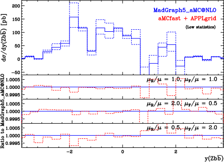
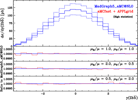
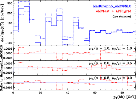
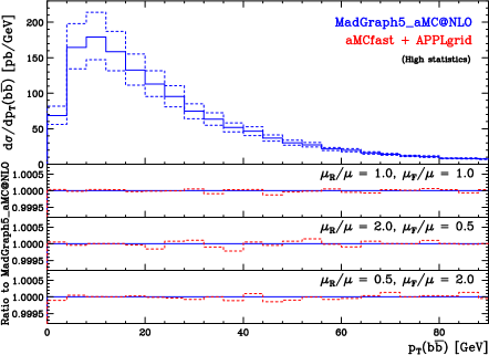
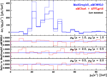
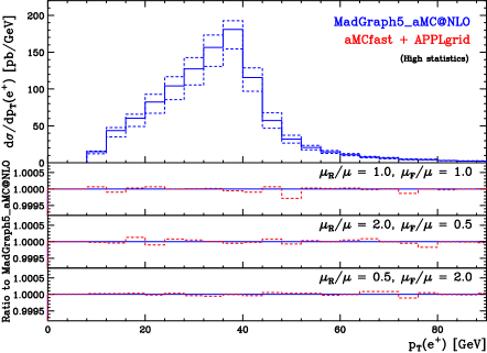
and as obtained from two different runs: one with “low” statistics, and one with “high” statistics. For each choice of scales and type of run, we shall plot the reference result, and the ratio of the reconstructed over the reference result. From that ratio, we shall see that the typical numerical inaccuracies due to the use of the interpolating grids are in the lower $10^{-4}$, with occasional larger differences in the case of the low-statistics runs, due to a still-insufficient amount of information stored in the grids. The crucial point is the following: even with very limited statistics, the reconstruction of the reference results is extremely good, and this for distributions whose quality is largely insufficient for any phenomenological application. This proves that, for all practical purposes, the level of agreement between reconstructed and reference results is independent of the statistics employed.

In keeping with the strategy at the core of all applications of MadGraph5_aMC@NLO, the only operations to be performed by the user when running with aMCfast are related to the process-specific analysis. In particular, in view of the fast interface to fNLO results, the user’s analysis (to be stored, as for any other kind of fNLO user utility, into the directory MYPROC/FixedOrderAnalysis – see sect. 3.2.2 of ref. [37] for more details) will need to contain, for each observable that he/she wants to consider, the instructions for filling the histogram that will contain the reference result (such instructions are identical to those of an fNLO analysis used when no interface with aMCfast is considered), and those for setting up the associated interpolating grids. Several templates of analyses that can be used with aMCfast will be provided in MYPROC/FixedOrderAnalysis (starting from the next version of MadGraph5_aMC@NLO), and the user should be able to easily adapt them to suit the needs of any given calculation. For the whole procedure to work, one will need to install, on top of MadGraph5_aMC@NLO and of the bridge code aMCfast, also APPLgrid version 1.4.56 or higher.

Parameter	value	Parameter	value
$\kappa$	5	$\Lambda$	0.250 GeV
$(x_{\min},x_{\max})$	$(2\!\cdot\!10^{-7},1)$	$(\mu_{\min},\mu_{\max})$	(10,3162) GeV
$N_{y}$	50	$N_{\tau}$	30
$s_{y}$	3	$s_{\tau}$	3

Table 1: Grid parameters used in the MadGraph5_aMC@NLO – aMCfast – APPLgrid validation runs presented here. In the case of $t\bar{t}$ production (sect. 3.2), the values of $\mu_{\max}$ and $N_{\tau}$ have been set equal to $10^{4}$ GeV and $50$, respectively.

All of the calculations reported below are carried out either with the default physics model of fNLO computations in MadGraph5_aMC@NLO, which corresponds to the SM with $N_{\scriptscriptstyle F}=4$ light flavours, or with its $N_{\scriptscriptstyle F}=5$ or $N_{\scriptscriptstyle F}=3$ variants; the quarks which are not light (the top and, depending on the value of $N_{\scriptscriptstyle F}$, the bottom and the charm) are given a non-zero mass. The parameters used to initialise the interpolating grids are given in table 1: from the first and second lines there, and by using eqs. (46) and (47), one immediately obtains the actual interpolation ranges in the variables $y_{i}$ and $\tau$, and the corresponding grid spacings by taking the ratio of those over $(N_{y}-1)$ and $(N_{\tau}-1)$, respectively. In the low- and high-statistics runs we employ a number of phase-space points per integration channel of the order of $10^{3}$ and $10^{6}$ respectively. For each process we shall consider a couple of observables to be definite, but we emphasise again that the number and the nature of the observables that one can compute are the user’s choice. The kinematical cuts will in general be similar to those used by ATLAS or CMS in some analogous experimental analyses; however, a comparison with experimental data is beyond the scope of this work. In all cases, we shall set $\mu=H_{\scriptscriptstyle T}/2$, with $H_{\scriptscriptstyle T}$ the scalar sum of the transverse energies of all the final-state particles. We point out that the choice of scales may have some implications on the settings of the corresponding interpolation parameters. For example, as one can see from table 1, in the case of $t\bar{t}$ production the values of $\mu_{\max}$ and $N_{\tau}$ have been increased w.r.t. those used for all the other processes, and this in order to attain a comparable numerical precision. On the other hand, we have verified that, by choosing scales which do not depend on the event kinematics, and are of the order of the hardness of the given process at threshold, setting $N_{\tau}=10$ is amply sufficient. To put things in perspective, however, we emphasise that even by using $N_{\tau}=30$ in $t\bar{t}$ production with $\mu=H_{\scriptscriptstyle T}/2$, numerical inaccuracies are at most $5\!\cdot\!10^{-4}$ and generally smaller than that, i.e. better than any PDF-fit application will ever need.

We start by studying top-quark pair production, which provides information on the gluon PDF in the large-$x$ region complementary to those provided by jet-production data. We shall then consider isolated-photon production in association with jets, a process that allows a variety of tests of perturbative QCD and that is also directly sensitive to the gluon PDF. We shall next discuss the production of a lepton pair in association with one extra hard jet. We shall then turn to considering $Zb\bar{b}$ production, a case-study of how the complete automation of fast NLO QCD calculations allows one to include in global PDF fits arbitrarily complicated processes at no significant extra cost. Finally, we shall discuss in some details another important process at the LHC for PDF extraction, namely the production of a $W$ boson in association with charm quarks, which is directly sensitive to the poorly known strange-quark PDF, and for which data from ATLAS and CMS have recently become available.

3.2 Top-quark pair production

Top-quark pair production provides one with unique information on the poorly known large-$x$ gluon PDF [23, 13, 35]. Unlike the case of the Tevatron, where $t\bar{t}$ production is mostly driven by $q\bar{q}$ scattering, at the LHC the $gg$-initiated process is dominant, contributing to more that 85% of the total inclusive cross section. The recent calculation of the total cross section to NNLO [54], as well as the upcoming NNLO results for differential distributions, make top-quark pair production an essential ingredient for present and future global PDF analyses. A wide range of data from the LHC for this process are available, both for inclusive cross-sections [55, 56, 57] and for differential distributions [58, 59], and much more will be measured in the near future.

As usual, the production of stable $t\bar{t}$ pairs in MadGraph5_aMC@NLO is simulated by starting with the generation of the process. Since in the default model used by MadGraph5_aMC@NLO there are four light flavours, one needs first to import a proper massless-bottom model. This is done by means of the following commands:

MG5_aMC>  import model loop_sm-no_b_mass

MG5_aMC>  define p = g u d s c b u~ d~ s~ c~ b~

Here, the second command instructs MadGraph5_aMC@NLO that the proton contains five light flavours, and does include the bottom quark; by doing so, partonic subprocesses will be generated that feature bottom quarks in the initial state. After this, one may proceed with the generation command;

MG5_aMC>  generate p p > t t~ [QCD]

followed by the standard output and launch commands (see sect. 3 of ref. [37] for more details). There are $n_{l}=7$ contributing parton luminosities. For each of them, we report in table 2

$l$	$n_{rs}$	$(r,s)$
1	1	$(g\,,g)$
2	5	$(\bar{b}\,,g)$	$(\bar{c}\,,g)$	$(\bar{s}\,,g)$	$(\bar{u}\,,g)$	$(\bar{d}\,,g)$
3	5	$(d\,,g)$	$(u\,,g)$	$(s\,,g)$	$(c\,,g)$	$(b\,,g)$
4	5	$(g\,,\bar{b})$	$(g\,,\bar{c})$	$(g\,,\bar{s})$	$(g\,,\bar{u})$	$(g\,,\bar{d})$
5	5	$(g\,,d)$	$(g\,,u)$	$(g\,,s)$	$(g\,,c)$	$(g\,,b)$
6	5	$(d\,,\bar{d})$	$(u\,,\bar{u})$	$(s\,,\bar{s})$	$(c\,,\bar{c})$	$(b\,,\bar{b})$
7	5	$(\bar{b}\,,b)$	$(\bar{c}\,,c)$	$(\bar{s}\,,s)$	$(\bar{u}\,,u)$	$(\bar{d}\,,d)$

Table 2: Values of $l$ and $(r,s)$ for which $T_{rs}^{(l)}=1$, as generated by aMCfast in $t\bar{t}$ production. For a given $l$, the number $n_{rs}$ of non-null terms in the sum on the r.h.s. of eq. (51) is also given.

Figure 1: Rapidity of the top quark, in $t\bar{t}$ production at the 14 TeV LHC, for a low- (left panel) and high-statistics (right panel) run. In the main frames we show the reference MadGraph5_aMC@NLO results obtained with central (eq. (63), solid histogram) and with non-central (eqs. (64) and (65), dashed histograms) scale choices. The three lower insets present the ratios of the reconstructed results over the corresponding reference result, for each of the three scale choices.

the corresponding $(r,s)$ contributions, which are the terms on the r.h.s. of eq. (51) with $T_{rs}^{(l)}=1$; the number of such terms, denoted by $n_{rs}$, is also reported in this table. As was already mentioned in sect. 2.3, the assignments of table 2 are automatically determined by aMCfast using the information provided by MadGraph5_aMC@NLO. We point out that each of the lines in table 2 corresponds to the set of four grids of eqs. (54)–(57). It is possible to use them separately, e.g. in order to determine the relative contribution of each parton luminosity to the different bins of the kinematical distributions studied, although this feature has not been used in this paper.

Figure 2: As in fig. 1, for the $t\bar{t}$ invariant mass.

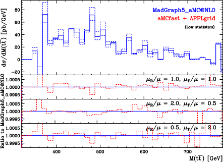
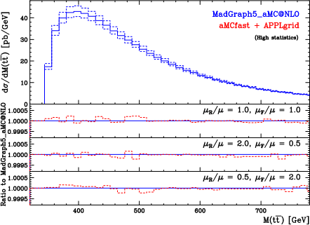
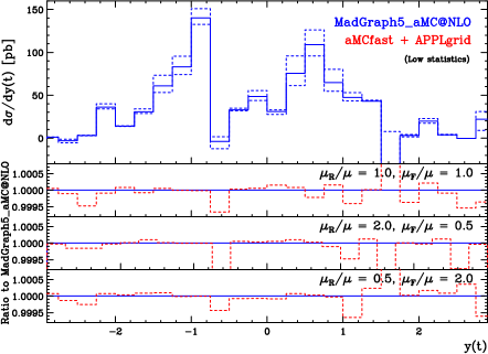
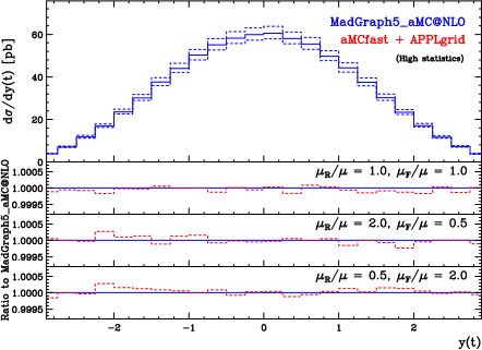
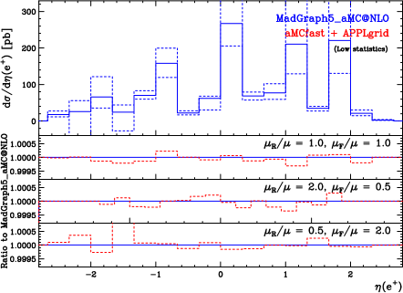
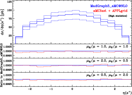
The results of our validation are presented in figs. 1 and 2, where we show the rapidity of the top quark ($y(t)$), and the $t\bar{t}$ invariant mass ($M(t\bar{t})$), respectively. Each figure consists of two panels, with that of the left (right) obtained with a low-statistics (high-statistics) run. Each panel has a main frame, where the solid histogram is the MadGraph5_aMC@NLO reference result obtained with the central scales of eq. (63), and the dashed histograms are the MadGraph5_aMC@NLO reference results relevant to the two non-central scale choices of eqs. (64) and (65) – incidentally, we note that the latter two predictions are obtained by using the reweighting technique presented in ref. [48] (i.e., MadGraph5_aMC@NLO has been run only once). The three lower insets show the accuracy obtained with interpolating grids, since they display as dashed histograms the ratio of the reconstructed over the reference result, for each of the three scale choices. These histograms thus represent the validation of the MadGraph5_aMC@NLO – aMCfast – APPLgrid chain, with values equal to one equivalent to a fast computation of the cross section with zero interpolation errors. As one can see from the plots, we obtain in all bins and for all scale choices an accuracy of $3\cdot 10^{-4}$ at worst in the case of the high-statistics run. In keeping with the general discussion given at the beginning of sect. 3, the reconstruction accuracy of the low-statistics results is also quite good, in spite of the fact that the corresponding differential cross sections display extremely large fluctuations, and are unsuitable for phenomenology.

3.3 Photon production in association with one jet

The production of direct photons in hadronic collisions is sensitive to the gluon PDF, owing to the dominance of QCD Compton-scattering-like diagrams. Thanks to tight isolation requirements applied to both theory prediction and data, one is able to significantly reduce or even eliminate completely the cross section of non-direct photons, due to poorly-known fragmentation-fuction contributions in the former, and to the contaminating $\pi^{0}\to\gamma\gamma$ decays in the latter. A recent re-analysis of all available isolated-photon collider data (inclusive in additional QCD radiation) has shown that NLO QCD gives a good description of all the data sets, and in addition it can provide one with some constraints on the gluon PDF in the region of Bjorken-$x$ relevant to the calculation of the gluon-fusion Higgs production cross section [22]. Therefore, there is a solid case to include photon data in the next generation of global PDF analyses. Data for isolated-photon production has been released by ATLAS and CMS [60, 61, 62]; in particular, the latest ATLAS measurement [60], that makes use of the complete 7 TeV run statistics, extends their kinematical coverage in the photon transverse energy up to a value of $E_{\scriptscriptstyle T}(\gamma)\sim 600$ GeV (see also ref. [63] for a study of the sensitivity of this measurement to various sets of PDFs).

On top of inclusive isolated-photon production, that of isolated photons in association with extra jets allows one to extend the sensitivity to the gluon PDF to a wider range of Bjorken-$x$, and also provides one with some information on the quark PDFs. Some measurements of isolated photon plus jets have been reported by ATLAS and CMS [64, 65, 66]; while these data are still not precise enough to directly constrain PDFs [67], the increase of the statistics collected in future LHC runs will dramatically change the picture, so that this process will become a useful addition to global PDF fits.

We have thus computed $\gamma+$jet production with MadGraph5_aMC@NLO. The computation is performed with five light flavours, so the generation command must be preceded by the same import and define commands which have been used in the case of $t\bar{t}$ production (see sect. 3.2). On top of those, we must also use here:

MG5_aMC>  define j = g u d s c b u~ d~ s~ c~ b~

since a light jet must have the same parton contents as the proton. The generation command is then:

MG5_aMC>  generate p p > a j [QCD]

We have imposed the photon to be hard and central, $p_{\scriptscriptstyle T}(\gamma)\geq 80$ GeV and $\left|\eta(\gamma)\right|\leq 3$. We use the Frixione photon-isolation prescription [68], since in this way one sets identically equal to zero the contribution of the fragmentation-function component in an infrared-safe manner.

Figure 3: As in fig. 1, for the photon transverse momentum, in the hadroproduction of an isolated photon in association with an extra jet.

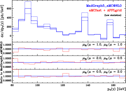
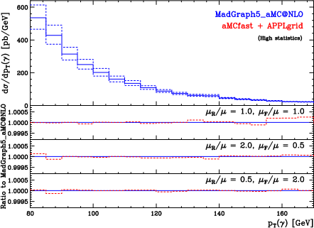
The parameters of the isolation (which in MadGraph5_aMC@NLO can be easily modified at the run-card level) are set as follows: $\epsilon_{\gamma}=1.0$ and $n=1$ (see eq. (3.4) of ref. [68]; note that, in an hadronic environment, the energies and angles of that equation have to be formally replaced by transverse energies and distances in the $(\eta,\varphi)$ plane); we use an isolation cone of radius $R_{0}=0.4$. Jets are reconstructed with the anti-$k_{\scriptscriptstyle T}$ algorithm [69], as implemented in FastJet [70], with a jet radius of $R=0.4$, and subject to the conditions $p_{\scriptscriptstyle T}(j)\geq 30$ GeV and $\left|\eta(j)\right|\leq 4.4$.

Figure 4: As in fig. 3, for the photon pseudorapidity.

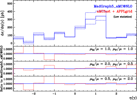
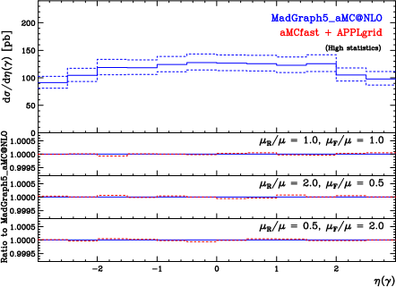
There are $n_{l}=33$ parton luminosities that contribute to the current process; their list is given in table 3 (see appendix A). That table shows that the definition of the parton luminosities in MadGraph5_aMC@NLO (i.e., eq. (50)) is not maximally efficient. For example, the matrix elements associated with $l=30$ and $l=31$ in table 3 are not equal, but differ by a trivial overall factor (the charge squared of a up-type vs an down-type quark). The combination of these two contributions could therefore be achieved by simply relaxing the condition that all non-zero $T_{rs}^{(l)}$ elements be equal to one. While this can easily be done in the context of a specific computation, its general implementation in an automated code able to deal with any user-defined process is not straightforward.

The validation plots, presented in figs. 3 and 4, follow the same pattern as those for $t\bar{t}$ production. The representative observables chosen here are the photon transverse momentum ($p_{\scriptscriptstyle T}(\gamma)$, fig. 3) and the photon pseudorapidity ($\eta(\gamma)$, fig. 4). As in sect. 3.2, the agreement between the reference and reconstructed results is at the level of $10^{-4}$ or better for the high-statistics run, and only slightly worse for the low-statistics one.

3.4 Dilepton production in association with one jet

We now turn to studying the hadroproduction of a lepton pair in association with one jet; the leptons originate from an intermediate virtual $Z$ or $\gamma$ boson, and we shall denote the pair with the shorthand notation $Z^{\star}$ in what follows. Inclusive $Z$-boson production has been used for a long time in PDF fits, since it provides one with a clean handle on the quark flavour separation in the proton, and various quality measurements from the Tevatron [71, 72] and the LHC [15, 73] are available. On the other hand, by requiring the presence of an additional extra jet one enters in a different domain, since at the Born level one is dominated by $qg$ channels, which thus allow one to probe directly the gluon PDF. In this context, it is convenient to study the large-$p_{\scriptscriptstyle T}(Z^{\star})$ region: in fact, the fraction of gluon-initiated events increases with $p_{\scriptscriptstyle T}(Z^{\star})$, and furthermore by doing so one is safely away from the small-$p_{\scriptscriptstyle T}(Z^{\star})$ region, where fixed-order calculations do not give physically-meaningful predictions. Another advantage associated with this kinematic region is that ratios of cross sections for $W$ over $Z$ production in association with jets can result in clean constraints on quarks and antiquarks PDFs at large-$x$ [26], where they are poorly known (and especially so for the antiquarks).

There are various ATLAS and CMS measurements available for $Z$+jets production, which typically focus on the comparison between theory and data as a test of perturbative-QCD predictions which are capable of describing a significant amount of hard radiation [74, 75, 76, 77]. However, from the PDF point of view, it is more interesting to perform the analysis as inclusively as possible (bar for the first jet, which one needs in order to be sensitive to the gluon PDF, as mentioned above), and to concentrate on the precise measurement of the $Z^{\star}$ transverse momentum, possibly in bins of different rapidity $y(Z^{\star})$. It is particularly convenient to perform such a measurement with a leptonically-decaying $Z$, which offers a cleaner scenario w.r.t. that of a hadronic decay; there are ongoing analyses in ATLAS and CMS – see e.g. [78].

We have computed dilepton$+$jet production at fNLO with MadGraph5_aMC@NLO in the five-flavour scheme, following the generation command:

MG5_aMC>  generate p p > mu+ mu- j [QCD]

which has been preceded by the same import and define commands relevant to sect. 3.3. We have also imposed the following cuts:

$$p_{\scriptscriptstyle T}(\mu^{\pm})\geq 10~{}{\rm GeV}\,,\;\;\;\;\;\;\left|\eta(\mu^{\pm})\right|\leq 2.5\,,\;\;\;\;\;\;M(\mu^{+}\mu^{-})\geq 20~{}{\rm GeV}\,.$$ (66)

The list of parton luminosities relevant to this process is the same as that for $\gamma+$jet production, and is given in table 3. As in the $\gamma+$jet case, jets are reconstructed by using the anti-$k_{t}$ algorithm with $R=0.4$, $p_{\scriptscriptstyle T}(j)\geq 30$ GeV, and $\left|\eta(j)\right|\leq 4.4$.

Figure 5: As in fig. 1, for the lepton-pair transverse momentum, in the hadroproduction of a lepton pair in association with an extra jet.

Figure 6: As in fig. 5, for the lepton-pair invariant mass.

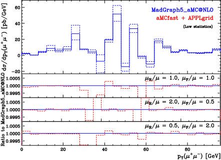
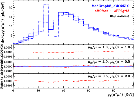
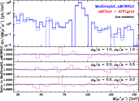
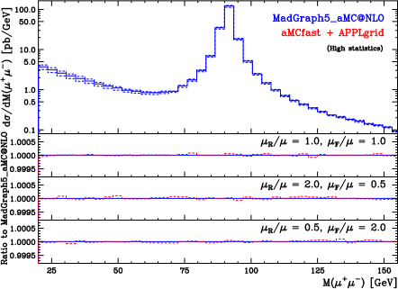
For the aMCfast validation we have chosen the transverse momentum of the lepton pair and its invariant mass, $p_{\scriptscriptstyle T}(\mu^{+}\mu^{-})$ and $M(\mu^{+}\mu^{-})$, which we display in figs. 5 and 6 respectively. The latter clearly shows the small-$M$ enhancement due to the presence of an intermediate photon. In the former, the feature around $p_{\scriptscriptstyle T}(\mu^{+}\mu^{-})\sim 30$ GeV is due to the presence of a sharp kinematic threshold only at the Born level (induced by the $p_{\scriptscriptstyle T}(j)$ cut), which causes this region to be infrared-sensitive [79]. Although this is an issue from the physics point of view for perturbative calculations, it does not pose any problems for the reconstruction through interpolating grids. We observe again an excellent agreement between the reference and the reconstructed results.

3.5 $Z$ production in association with a $b\bar{b}$ pair

The production of a $Z$ boson in association with a bottom-antibottom quark pair is an interesting example of how the automation of a fast interface to NLO QCD computations achieved by aMCfast can be a valuable tool to easily include arbitrarily complicated process into a global PDF fit. A related application could be that of studying to which degree the recent discrepancies between theory and experiment (see e.g. ref. [80]) for the production of $Z$ bosons in association with bottom quarks might be absorbed by a change in PDFs. The hadroproduction of $Wb\bar{b}$ and $(Z/\gamma^{*})b\bar{b}$ in the MadGraph5_aMC@NLO framework has been previously discussed in ref. [81], without however considering any aspects relevant to PDFs.

The generation of the current process in MadGraph5_aMC@NLO is achieved through the command:

MG5_aMC>  generate p p > z b b~ [QCD]

Note that the default model adopted by MadGraph5_aMC@NLO for NLO computations treats the bottom quarks as massive particles, and one works in a four-flavour scheme: hence, no models are explicitly imported, and no multi-particle labels redefined, at variance with was done previously. This is important in order to be able to perform the computation of $Zb\bar{b}$ production without resorting to any kind of jet-reconstruction algorithm, to probe the $b$ quarks down to zero transverse momentum, and to define a fully-inclusive cross section. The list of partonic luminosities that contribute to this process is given in table 4.

Figure 7: As in fig. 1, for the rapidity of the $Zb\bar{b}$ system, in $Zb\bar{b}$ hadroproduction.

We validate the results of the present simulation by considering the rapidity distribution of the $Zb\bar{b}$ system (shown in fig. 7), and the transverse momentum of the $b\bar{b}$ pair (shown in fig. 8). As in the previous cases, we observe no significant deviations of the reconstructed from the reference predictions.

3.6 $W$ production in association with charm quarks

The final representative example of an LHC process of interest for PDF fits that we discuss in this work is the hadroproduction of $W$ bosons in association with charm quarks. This process is directly sensitive to the PDF of the strange quark (see e.g. refs. [82, 83]), which among the light-quark PDFs is the most poorly determined. In the majority of global PDF fits, the strange PDF is constrained by neutrino data [84, 85, 86] (in particular by the so-called dimuon process, i.e. charm production in charged-current DIS). The use of neutrino DIS data in PDF fits has several drawbacks, such as the need to model charm fragmentation, and to understand charm-quark mass effects at low scales.

Figure 8: As in fig. 7, for the transverse momentum of the $b\bar{b}$ pair.

It is therefore quite interesting that $Wc$ hadron-collider data provide one with a clean and robust independent check of the strange PDF determined elsewhere. In addition to that, the differences in the production rates of $W^{+}$ and $W^{-}$ bosons in association with charm quarks give information on the strange asymmetry in the proton, that plays an important role in the explanation [87] of the NuTeV anomaly [86]. Data on $W$ production in association with either charm jets or $D$ mesons have been made public by ATLAS [88] and CMS [24], based on the 7 TeV 2011 data sets, and analogous measurements from the 8 TeV run are ongoing. In particular, the CMS $Wc$ data has been recently used in a QCD analysis [16], together with HERA data, to show that the strange-quark PDF from collider-only data can be determined with a precision comparable to that of global fits which include neutrino data. Another recent analysis of the compatibility of the LHC $Wc$ data with existing fixed-target DIS and Drell-Yan data has been presented in ref. [89].

Once again, we now compare a couple of reference distributions from MadGraph5_aMC@NLO to those obtained with the a-posteriori aMCfast – APPLgrid convolution. For simplicity, we restrict ourselves to considering $W^{+}\bar{c}$ production; on the other hand, the process we shall actually deal with is that where an electron and a neutrino, rather than a $W$, are present in the final state, so as to make sure that all production spin correlations are correctly taken into account. Incidentally, this also shows that one is not restricted to performing computations in the narrow width approximation; in particular, the complex mass scheme [90] is fully supported in MadGraph5_aMC@NLO. Similarly to the case of the $b$ quark in $Zb\bar{b}$ production discussed in sect. 3.5, in the present case it is best to treat the charm as a massive particle. Since in the default model used by MadGraph5_aMC@NLO the charm is massless, one needs to import a proper massive-charm model before proceeding with the generation of the process. This is done by means of the following commands:

MG5_aMC>  import model loop_sm-c_mass

MG5_aMC>  define p = g u d s u~ d~ s~

MG5_aMC>  generate p p > e+ ve c~ [QCD]

In this list, the second command instructs MadGraph5_aMC@NLO that the proton contains three light flavours, and does not feature the charm quark; by doing so, no partonic subprocesses will be generated that feature a charm in the initial state. The following cuts have been imposed:

$$p_{\scriptscriptstyle T}(e^{+})\geq 10~{}{\rm GeV}\,,\;\;\;\;\;\;\left|\eta(e^{+})\right|\leq 2.5\,.$$ (67)

The list of partonic luminosities that contribute to this process in given in table 5.

The two representative distributions that we use for validation are the pseudorapidity of the positron, ($\eta(e^{+})$, presented in fig. 9), and its transverse momentum ($p_{\scriptscriptstyle T}(e^{+})$ , presented in fig. 10). The same conclusions as in all previous cases apply here.

4 Conclusions and outlook

In this paper we have presented aMCfast, a tool that serves to achieve the complete automation of fast NLO QCD computations for arbitrary processes, by constructing a bridge between MadGraph5_aMC@NLO, which performs the core automated cross section calculations, and APPLgrid, which allows one to represent a given observable in term of interpolating grids that can be used for a fast and a-posteriori evaluation, and one in which the possibility is given of changing the scales and PDFs w.r.t. those used in the original computation. Since fast calculations of NLO cross sections are an absolute necessity in the context of global PDF fits, the combination of the automated programs discussed in this paper covers all the present and, more importantly, future needs relevant to PDF analyses.

Figure 9: As in fig. 1, for the $e^{+}$ pseudorapidity, in $W^{+}\bar{c}$ hadroproduction.

We have validated our approach by considering a representative sample of production processes at the LHC (some of which not previously available in the form of fast computations), and by comparing for several observables the bin-by-bin agreement between the original results of MadGraph5_aMC@NLO, and those reconstructed by means of aMCfast and APPLgrid. The typical accuracy that we find is of the order of some parts in $10^{-4}$, which is in fact far more than sufficient for any kind of phenomenological application. Moreover, our approach allows one to consider scale variations without any loss of precision, and without the need for interfacing APPLgrid with an external program to perfom PDF evolution.

A natural outcome of this work is the use of the grids produced using aMCfast in actual global PDF analyses, in view of the possible inclusion into the latter of LHC data, and especially of those which have not been considered so far, for lack of either sufficiently precise measurements, or of theoretical NLO calculations suited to the task. Given that the format of the results of the aMCfast – APPLgrid interface is a trivial extension of that produced by APPLgrid interfaced with other codes, aMCfast should be straighforward to employ by the global-PDF fitters already experienced with the former code.

The outlook for the near future features two important developments.

Figure 10: As in fig. 9, for the $e^{+}$ transverse momentum.

Firstly, there is no conceptual difference between what has been done here, and its analogue in the case of a perturbative expansion in either the electroweak coupling constant $\alpha$, or simultaneously in $\alpha_{\scriptscriptstyle S}$ and $\alpha$ (mixed-coupling expansion). From the technical viewpoint, the only implication of a mixed-coupling expansion is the necessity of introducing additional interpolating grids, which is trivial. This point is important in view of the fact that MadGraph5_aMC@NLO is expected to be able to handle soon both kind of computations; thus, any extension of the MadGraph5_aMC@NLO capabilities will be made immediately available for fast computations, thanks to straightforward modifications to aMCfast. This will pave the way to a systematic inclusion of electroweak NLO corrections into global PDF fits; cases where such an inclusion may prove particularly relevant include high-$p_{\scriptscriptstyle T}$ jet production, the high-mass Drell-Yan cross section, as well as the consistent treatment of photon-initiated processes that are necessary for the determination of the photon PDF [91]. Secondly, the scale- and PDF-independent coefficients computed by MadGraph5_aMC@NLO, and used by aMCfast to set up the interpolating grids at fixed order, are quite similar to those relevant to the MC@NLO short-distance cross sections. Therefore, the current structure of aMCfast will need only a minor upgrade to be able to deal with NLO+PS computations. Apart from its obvious phenomenological spinoffs, and the possibility of obtaining PDF fits that include resummation effects well tuned to experimental data, such a project is also interesting from a more theoretical viewpoint, in that it would help spur a thorough investigation of the effects of the PDFs in initial-state showers; there is some evidence that these effects are small, but more systematic studies should be carried out, in view of the fact that they cannot be taken into account by any method based solely on short-distance cross section information.

The public version of the aMCfast code will soon be available at:
     http://amcfast.hepforge.org/
Meanwhile, potential users are kindly requested to contact the authors.

Appendix A Luminosity factors

In this appendix, we report the luminosity indices $l$ and parton identities $(r,s)$ for which the quantity $T_{rs}^{(l)}$ that enters eq. (51) is equal to one. We do so for all of the processes studied in sect. 3, except for $t\bar{t}$ production, whose analogous information have already been given in sect. 3.

$l$	$n_{rs}$	$(r,s)$
1	2	$(g\,,u)$	$(g\,,c)$
2	6	$(\bar{b}\,,u)$	$(\bar{b}\,,c)$	$(\bar{s}\,,u)$	$(\bar{s}\,,c)$	$(\bar{d}\,,u)$	$(\bar{d}\,,c)$
3	6	$(d\,,u)$	$(d\,,c)$	$(s\,,u)$	$(s\,,c)$	$(b\,,u)$	$(b\,,c)$
4	2	$(\bar{c}\,,c)$	$(\bar{u}\,,u)$
5	2	$(u\,,u)$	$(c\,,c)$
6	2	$(\bar{c}\,,u)$	$(\bar{u}\,,c)$
7	2	$(u\,,c)$	$(c\,,u)$
8	1	$(g\,,g)$
9	3	$(g\,,d)$	$(g\,,s)$	$(g\,,b)$
10	3	$(\bar{b}\,,b)$	$(\bar{s}\,,s)$	$(\bar{d}\,,d)$
11	3	$(d\,,d)$	$(s\,,s)$	$(b\,,b)$
12	6	$(\bar{c}\,,d)$	$(\bar{c}\,,s)$	$(\bar{c}\,,b)$	$(\bar{u}\,,d)$	$(\bar{u}\,,s)$	$(\bar{u}\,,b)$
13	6	$(u\,,d)$	$(u\,,s)$	$(u\,,b)$	$(c\,,d)$	$(c\,,s)$	$(c\,,b)$
14	6	$(\bar{b}\,,d)$	$(\bar{b}\,,s)$	$(\bar{s}\,,d)$	$(\bar{s}\,,b)$	$(\bar{d}\,,s)$	$(\bar{d}\,,b)$
15	6	$(d\,,s)$	$(d\,,b)$	$(s\,,d)$	$(s\,,b)$	$(b\,,d)$	$(b\,,s)$
16	2	$(g\,,\bar{c})$	$(g\,,\bar{u})$
17	6	$(\bar{b}\,,\bar{c})$	$(\bar{b}\,,\bar{u})$	$(\bar{s}\,,\bar{c})$	$(\bar{s}\,,\bar{u})$	$(\bar{d}\,,\bar{c})$	$(\bar{d}\,,\bar{u})$
18	6	$(d\,,\bar{c})$	$(d\,,\bar{u})$	$(s\,,\bar{c})$	$(s\,,\bar{u})$	$(b\,,\bar{c})$	$(b\,,\bar{u})$
19	2	$(\bar{c}\,,\bar{c})$	$(\bar{u}\,,\bar{u})$
20	2	$(u\,,\bar{u})$	$(c\,,\bar{c})$
21	2	$(\bar{c}\,,\bar{u})$	$(\bar{u}\,,\bar{c})$
22	2	$(u\,,\bar{c})$	$(c\,,\bar{u})$
23	3	$(g\,,\bar{b})$	$(g\,,\bar{s})$	$(g\,,\bar{d})$
24	3	$(\bar{b}\,,\bar{b})$	$(\bar{s}\,,\bar{s})$	$(\bar{d}\,,\bar{d})$
25	3	$(d\,,\bar{d})$	$(s\,,\bar{s})$	$(b\,,\bar{b})$
26	6	$(\bar{c}\,,\bar{b})$	$(\bar{c}\,,\bar{s})$	$(\bar{c}\,,\bar{d})$	$(\bar{u}\,,\bar{b})$	$(\bar{u}\,,\bar{s})$	$(\bar{u}\,,\bar{d})$
27	6	$(u\,,\bar{b})$	$(u\,,\bar{s})$	$(u\,,\bar{d})$	$(c\,,\bar{b})$	$(c\,,\bar{s})$	$(c\,,\bar{d})$
28	6	$(\bar{b}\,,\bar{s})$	$(\bar{b}\,,\bar{d})$	$(\bar{s}\,,\bar{b})$	$(\bar{s}\,,\bar{d})$	$(\bar{d}\,,\bar{b})$	$(\bar{d}\,,\bar{s})$
29	6	$(d\,,\bar{b})$	$(d\,,\bar{s})$	$(s\,,\bar{b})$	$(s\,,\bar{d})$	$(b\,,\bar{s})$	$(b\,,\bar{d})$
30	2	$(u\,,g)$	$(c\,,g)$
31	3	$(d\,,g)$	$(s\,,g)$	$(b\,,g)$
32	2	$(\bar{c}\,,g)$	$(\bar{u}\,,g)$
33	3	$(\bar{b}\,,g)$	$(\bar{s}\,,g)$	$(\bar{d}\,,g)$

Table 3: As in table 2, for $\gamma+$jet and dilepton$+$jet production.

$l$	$n_{rs}$	$(r,s)$
1	1	$(g\,,g)$
2	2	$(\bar{s}\,,g)$	$(\bar{d}\,,g)$
3	2	$(d\,,g)$	$(s\,,g)$
4	2	$(\bar{c}\,,g)$	$(\bar{u}\,,g)$
5	2	$(u\,,g)$	$(c\,,g)$
6	2	$(g\,,\bar{s})$	$(g\,,\bar{d})$
7	2	$(g\,,d)$	$(g\,,s)$
8	2	$(g\,,\bar{c})$	$(g\,,\bar{u})$
9	2	$(g\,,u)$	$(g\,,c)$
10	2	$(u\,,\bar{u})$	$(c\,,\bar{c})$
11	2	$(d\,,\bar{d})$	$(s\,,\bar{s})$
12	2	$(\bar{c}\,,c)$	$(\bar{u}\,,u)$
13	2	$(\bar{s}\,,s)$	$(\bar{d}\,,d)$

Table 4: As in table 2, for $Zb\bar{b}$ production.

$l$	$n_{rs}$	$(r,s)$
1	1	$(g\,,\bar{s})$
2	2	$(u\,,\bar{s})$	$(d\,,\bar{s})$
3	2	$(\bar{d}\,,\bar{s})$	$(\bar{u}\,,\bar{s})$
4	1	$(s\,,\bar{s})$
5	1	$(\bar{s}\,,\bar{s})$
6	1	$(g\,,g)$
7	1	$(\bar{s}\,,g)$
8	2	$(\bar{s}\,,u)$	$(\bar{s}\,,d)$
9	2	$(\bar{s}\,,\bar{d})$	$(\bar{s}\,,\bar{u})$
10	1	$(\bar{s}\,,s)$

Table 5: As in table 2, for $e^{+}\nu_{e}\bar{c}$ production.

References

- [1] S. Forte and G. Watt, Progress in the Determination of the Partonic Structure of the Proton, arXiv:1301.6754.
- [2] R. D. Ball, S. Carrazza, L. Del Debbio, S. Forte, J. Gao, et al., Parton Distribution Benchmarking with LHC Data, JHEP 1304 (2013) 125, [arXiv:1211.5142].
- [3] E. Perez and E. Rizvi, The Quark and Gluon Structure of the Proton, Rep.Prog.Phys. 76 (2013) 046201, [arXiv:1208.1178].
- [4] S. Forte, Parton distributions at the dawn of the LHC, Acta Phys.Polon. B41 (2010) 2859–2920, [arXiv:1011.5247].
- [5] A. De Roeck and R. Thorne, Structure Functions, Prog.Part.Nucl.Phys. 66 (2011) 727–781, [arXiv:1103.0555].
- [6] LHC Higgs Cross Section Working Group, S. Dittmaier et al., Handbook of LHC Higgs Cross Sections: 1. Inclusive Observables, arXiv:1101.0593.
- [7] LHeC Study Group, J. Abelleira Fernandez et al., On the Relation of the LHeC and the LHC, arXiv:1211.5102.
- [8] G. Bozzi, J. Rojo, and A. Vicini, The Impact of PDF uncertainties on the measurement of the W boson mass at the Tevatron and the LHC, Phys.Rev. D83 (2011) 113008, [arXiv:1104.2056].
- [9] J. Rojo, PDF uncertainties in the determination of the W boson mass and of the effective lepton mixing angle at the LHC, arXiv:1305.4833.
- [10] A. D. Martin, W. J. Stirling, R. S. Thorne, and G. Watt, Parton distributions for the LHC, Eur. Phys. J. C63 (2009) 189–285, [arXiv:0901.0002].
- [11] The NNPDF Collaboration, R. D. Ball et al., A first unbiased global NLO determination of parton distributions and their uncertainties, Nucl. Phys. B838 (2010) 136–206, [arXiv:1002.4407].
- [12] J. Gao, M. Guzzi, J. Huston, H.-L. Lai, Z. Li, et al., The CT10 NNLO Global Analysis of QCD, Phys.Rev. D89 (2014) 033009, [arXiv:1302.6246].
- [13] S. Alekhin, J. Bluemlein, and S. Moch, The ABM parton distributions tuned to LHC data, Phys.Rev. D89 (2014) 054028, [arXiv:1310.3059].
- [14] ZEUS Collaboration, H1 Collaboration, A. Cooper-Sarkar, PDF Fits at HERA, PoS EPS-HEP2011 (2011) 320, [arXiv:1112.2107].
- [15] ATLAS Collaboration, G. Aad et al., Measurement of the inclusive W+- and Z/gamma cross sections in the electron and muon decay channels in pp collisions at sqrt(s) = 7 TeV with the ATLAS detector, Phys.Rev. D85 (2012) 072004, [arXiv:1109.5141].
- [16] CMS Collaboration, S. Chatrchyan et al., Measurement of the muon charge asymmetry in inclusive pp W + X production at =7 TeV and an improved determination of light parton distribution functions, arXiv:1312.6283.
- [17] ATLAS Collaboration, G. Aad et al., Measurement of inclusive jet and dijet production in pp collisions at sqrt(s) = 7 TeV using the ATLAS detector, Phys. Rev. D86 (2012) 014022, [arXiv:1112.6297].
- [18] CMS Collaboration, S. Chatrchyan et al., Measurements of differential jet cross sections in proton-proton collisions at TeV with the CMS detector, Phys.Rev. D87 (2013) 112002, [arXiv:1212.6660].
- [19] ATLAS Collaboration, G. Aad et al., Measurement of dijet cross sections in pp collisions at 7 TeV centre-of-mass energy using the ATLAS detector, arXiv:1312.3524.
- [20] ATLAS, G. Aad et al., Measurement of the inclusive jet cross section in pp collisions at sqrt(s)=2.76 TeV and comparison to the inclusive jet cross section at sqrt(s)=7 TeV using the ATLAS detector, Eur.Phys.J. C73 (2013) 2509, [arXiv:1304.4739].
- [21] B. Watt, P. Motylinski, and R. Thorne, The Effect of LHC Jet Data on MSTW PDFs, arXiv:1311.5703.
- [22] D. d’Enterria and J. Rojo, Quantitative constraints on the gluon distribution function in the proton from collider isolated-photon data, Nucl.Phys. B860 (2012) 311–338, [arXiv:1202.1762].
- [23] M. Czakon, M. L. Mangano, A. Mitov, and J. Rojo, Constraints on the gluon PDF from top quark pair production at hadron colliders, JHEP 1307 (2013) 167, [arXiv:1303.7215].
- [24] CMS Collaboration, S. Chatrchyan et al., Measurement of associated W + charm production in pp collisions at = 7 TeV, arXiv:1310.1138.
- [25] CMS, S. Chatrchyan et al., Measurement of the differential and double-differential Drell-Yan cross sections in proton-proton collisions at 7 TeV, JHEP 1312 (2013) 030, [arXiv:1310.7291].
- [26] S. A. Malik and G. Watt, Ratios of W and Z cross sections at large boson as a constraint on PDFs and background to new physics, JHEP 1402 (2014) 025, [arXiv:1304.2424].
- [27] M. L. Mangano and J. Rojo, Cross Section Ratios between different CM energies at the LHC: opportunities for precision measurements and BSM sensitivity, JHEP 1208 (2012) 010, [arXiv:1206.3557].
- [28] G. P. Salam and J. Rojo, A Higher Order Perturbative Parton Evolution Toolkit (HOPPET), Comput. Phys. Commun. 180 (2009) 120–156, [arXiv:0804.3755].
- [29] M. Botje, QCDNUM: Fast QCD Evolution and Convolution, Comput.Phys.Commun. 182 (2011) 490–532, [arXiv:1005.1481].
- [30] V. Bertone, S. Carrazza, and J. Rojo, APFEL: A PDF Evolution Library with QED corrections, arXiv:1310.1394.
- [31] T. Kluge, K. Rabbertz, and M. Wobisch, Fast pQCD calculations for PDF fits, hep-ph/0609285.
- [32] fastNLO Collaboration, M. Wobisch, D. Britzger, T. Kluge, K. Rabbertz, and F. Stober, Theory-Data Comparisons for Jet Measurements in Hadron-Induced Processes, arXiv:1109.1310.
- [33] T. Carli, D. Clements, A. Cooper-Sarkar, C. Gwenlan, G. P. Salam, et al., A posteriori inclusion of parton density functions in NLO QCD final-state calculations at hadron colliders: The APPLGRID Project, Eur.Phys.J. C66 (2010) 503–524, [arXiv:0911.2985].
- [34] Z. Nagy, Three jet cross-sections in hadron hadron collisions at next-to-leading order, Phys.Rev.Lett. 88 (2002) 122003, [hep-ph/0110315].
- [35] M. Guzzi, K. Lipka, and S.-O. Moch, Top-quark pair production at hadron colliders: differential cross section and phenomenological applications with DiffTop, arXiv:1406.0386.
- [36] J. Campbell and R. K. Ellis, Next-to-leading order corrections to W + 2jet and Z + 2jet production at hadron colliders, Phys. Rev. D65 (2002) 113007, [hep-ph/0202176].
- [37] J. Alwall, R. Frederix, S. Frixione, V. Hirschi, F. Maltoni, et al., The automated computation of tree-level and next-to-leading order differential cross sections, and their matching to parton shower simulations, arXiv:1405.0301.
- [38] L. Del Debbio, N. P. Hartland, and S. Schumann, MCgrid: projecting cross section calculations on grids, arXiv:1312.4460.
- [39] A. Buckley, J. Butterworth, L. Lonnblad, D. Grellscheid, H. Hoeth, et al., Rivet user manual, Comput.Phys.Commun. 184 (2013) 2803–2819, [arXiv:1003.0694].
- [40] S. Frixione, Z. Kunszt, and A. Signer, Three jet cross-sections to next-to-leading order, Nucl.Phys. B467 (1996) 399–442, [hep-ph/9512328].
- [41] S. Frixione, A General approach to jet cross-sections in QCD, Nucl.Phys. B507 (1997) 295–314, [hep-ph/9706545].
- [42] R. Frederix, S. Frixione, F. Maltoni, and T. Stelzer, Automation of next-to-leading order computations in QCD: The FKS subtraction, JHEP 0910 (2009) 003, [arXiv:0908.4272].
- [43] G. Ossola, C. G. Papadopoulos, and R. Pittau, Reducing full one-loop amplitudes to scalar integrals at the integrand level, Nucl.Phys. B763 (2007) 147–169, [hep-ph/0609007].
- [44] V. Hirschi, R. Frederix, S. Frixione, M. V. Garzelli, F. Maltoni, et al., Automation of one-loop QCD corrections, JHEP 1105 (2011) 044, [arXiv:1103.0621].
- [45] G. Ossola, C. G. Papadopoulos, and R. Pittau, CutTools: A Program implementing the OPP reduction method to compute one-loop amplitudes, JHEP 0803 (2008) 042, [arXiv:0711.3596].
- [46] F. Cascioli, P. Maierhofer, and S. Pozzorini, Scattering Amplitudes with Open Loops, Phys.Rev.Lett. 108 (2012) 111601, [arXiv:1111.5206].
- [47] S. Frixione and B. R. Webber, Matching NLO QCD computations and parton shower simulations, JHEP 0206 (2002) 029, [hep-ph/0204244].
- [48] R. Frederix, S. Frixione, V. Hirschi, F. Maltoni, R. Pittau, et al., Four-lepton production at hadron colliders: aMC@NLO predictions with theoretical uncertainties, JHEP 1202 (2012) 099, [arXiv:1110.4738].
- [49] R. K. Ellis and J. Sexton, QCD Radiative Corrections to Parton Parton Scattering, Nucl.Phys. B269 (1986) 445.
- [50] G. Altarelli and G. Parisi, Asymptotic Freedom in Parton Language, Nucl.Phys. B126 (1977) 298.
- [51] R. D. Ball, V. Bertone, S. Carrazza, C. S. Deans, L. Del Debbio, et al., Parton distributions with LHC data, Nucl.Phys. B867 (2013) 244–289, [arXiv:1207.1303].
- [52] R. D. Ball, V. Bertone, F. Cerutti, L. Del Debbio, S. Forte, et al., Impact of Heavy Quark Masses on Parton Distributions and LHC Phenomenology, Nucl.Phys. B849 (2011) 296–363, [arXiv:1101.1300].
- [53] D. Bourilkov, R. C. Group, and M. R. Whalley, LHAPDF: PDF use from the Tevatron to the LHC, hep-ph/0605240.
- [54] M. Czakon, P. Fiedler, and A. Mitov, The total top quark pair production cross-section at hadron colliders through , Phys.Rev.Lett. 110 (2013) 252004, [arXiv:1303.6254].
- [55] The ATLAS Collaboration, Measurement of the top quark-pair production cross section with ATLAS in pp collisions at TeV, arXiv:1012.1792.
- [56] CMS Collaboration, S. Chatrchyan et al., Measurement of the production cross section in the dilepton channel in pp collisions at = 8 TeV, JHEP 1402 (2014) 024, [arXiv:1312.7582].
- [57] ATLAS Collaboration, G. Aad et al., Measurement of the top quark pair cross section with ATLAS in pp collisions at sqrt(s) = 7 TeV using final states with an electron or a muon and a hadronically decaying lepton, Phys.Lett. B717 (2012) 89–108, [arXiv:1205.2067].
- [58] CMS Collaboration, S. Chatrchyan et al., Measurement of differential top-quark pair production cross sections in colisions at TeV, Eur.Phys.J. C73 (2013) 2339, [arXiv:1211.2220].
- [59] ATLAS Collaboration, G. Aad et al., Measurements of top quark pair relative differential cross-sections with ATLAS in collisions at TeV, Eur.Phys.J. C73 (2013) 2261, [arXiv:1207.5644].
- [60] ATLAS Collaboration, G. Aad et al., Measurement of the inclusive isolated prompt photon cross section in pp collisions at = 7 TeV with the ATLAS detector using 4.6 fb-1, Phys.Rev. D89 (2014) 052004, [arXiv:1311.1440].
- [61] CMS Collaboration, S. Chatrchyan et al., Measurement of the Differential Cross Section for Isolated Prompt Photon Production in pp Collisions at 7 TeV, Phys.Rev. D84 (2011) 052011, [arXiv:1108.2044].
- [62] CMS Collaboration, V. Khachatryan et al., Measurement of the Isolated Prompt Photon Production Cross Section in Collisions at TeV, Phys.Rev.Lett. 106 (2011) 082001, [arXiv:1012.0799].
- [63] A study of the sensitivity to the proton parton distributions of the inclusive photon production cross section in collisions at 7 TeV measured by the ATLAS experiment at the LHC, Tech. Rep. ATL-PHYS-PUB-2013-018, CERN, Geneva, Dec, 2013.
- [64] ATLAS Collaboration, G. Aad et al., Dynamics of isolated-photon plus jet production in pp collisions at TeV with the ATLAS detector, Nucl.Phys. B875 (2013) 483–535, [arXiv:1307.6795].
- [65] CMS Collaboration, S. Chatrchyan et al., Rapidity distributions in exclusive Z + jet and + jet events in pp collisions at =7 TeV, Phys.Rev. D88 (2013) 112009, [arXiv:1310.3082].
- [66] CMS Collaboration, S. Chatrchyan et al., Measurement of the triple-differential cross section for photon+jets production in proton-proton collisions at =7 TeV, arXiv:1311.6141.
- [67] L. Carminati, G. Costa, D. D’Enterria, I. Koletsou, G. Marchiori, et al., Sensitivity of the LHC isolated-gamma+jet data to the parton distribution functions of the proton, EPL 101 (2013) 61002, [arXiv:1212.5511].
- [68] S. Frixione, Isolated photons in perturbative QCD, Phys.Lett. B429 (1998) 369–374, [hep-ph/9801442].
- [69] M. Cacciari, G. P. Salam, and G. Soyez, The Anti-k(t) jet clustering algorithm, JHEP 0804 (2008) 063, [arXiv:0802.1189].
- [70] M. Cacciari, G. P. Salam, and G. Soyez, FastJet User Manual, Eur.Phys.J. C72 (2012) 1896, [arXiv:1111.6097].
- [71] CDF, T. A. Aaltonen et al., Measurement of of Drell-Yan pairs in the Mass Region from Collisions at TeV, Phys. Lett. B692 (2010) 232–239, [arXiv:0908.3914].
- [72] D0, V. M. Abazov et al., Measurement of the shape of the boson rapidity distribution for + events produced at of 1.96-TeV, Phys. Rev. D76 (2007) 012003, [hep-ex/0702025].
- [73] CMS Collaboration, S. Chatrchyan et al., Measurement of the Rapidity and Transverse Momentum Distributions of Bosons in Collisions at TeV, Phys.Rev. D85 (2012) 032002, [arXiv:1110.4973].
- [74] ATLAS Collaboration, G. Aad et al., Measurement of the production cross section of jets in association with a Z boson in pp collisions at = 7 TeV with the ATLAS detector, JHEP 1307 (2013) 032, [arXiv:1304.7098].
- [75] ATLAS Collaboration, G. Aad et al., Measurement of the production cross section for Z/gamma* in association with jets in collisions at TeV with the ATLAS detector, Phys.Rev. D85 (2012) 032009, [arXiv:1111.2690].
- [76] CMS Collaboration, S. Chatrchyan et al., Event shapes and azimuthal correlations in + jets events in collisions at TeV, Phys.Lett. B722 (2013) 238–261, [arXiv:1301.1646].
- [77] CMS Collaboration, Jet multiplicity and differential production cross sections of Z+jets events in proton-proton collisions at 7 TeV, Tech. Rep. CMS-PAS-SMP-12-017, CERN, Geneva, 2014.
- [78] CMS Collaboration, Measurement of Z production as a function of pT, Y, Tech. Rep. CMS-PAS-SMP-13-013, CERN, Geneva, 2014.
- [79] S. Catani and B. Webber, Infrared safe but infinite: Soft gluon divergences inside the physical region, JHEP 9710 (1997) 005, [hep-ph/9710333].
- [80] CMS Collaboration, S. Chatrchyan et al., Measurement of the production cross sections for a Z boson and one or more b jets in pp collisions at = 7 TeV, arXiv:1402.1521.
- [81] R. Frederix, S. Frixione, V. Hirschi, F. Maltoni, R. Pittau, et al., W and boson production in association with a bottom-antibottom pair, JHEP 1109 (2011) 061, [arXiv:1106.6019].
- [82] U. Baur, F. Halzen, S. Keller, M. L. Mangano, and K. Riesselmann, The Charm content of + 1 jet events as a probe of the strange quark distribution function, Phys.Lett. B318 (1993) 544–548, [hep-ph/9308370].
- [83] W. Stirling and E. Vryonidou, Charm production in association with an electroweak gauge boson at the LHC, Phys.Rev.Lett. 109 (2012) 082002, [arXiv:1203.6781].
- [84] D. A. Mason, Measurement of the strange - antistrange asymmetry at NLO in QCD from NuTeV dimuon data, . FERMILAB-THESIS-2006-01.
- [85] D. Mason et al., Measurement of the Nucleon Strange-Antistrange Asymmetry at Next-to-Leading Order in QCD from NuTeV Dimuon Data, Phys. Rev. Lett. 99 (2007) 192001.
- [86] NuTeV Collaboration, M. Goncharov et al., Precise measurement of dimuon production cross-sections in muon neutrino Fe and muon anti-neutrino Fe deep inelastic scattering at the Tevatron, Phys.Rev. D64 (2001) 112006, [hep-ex/0102049].
- [87] The NNPDF Collaboration, R. D. Ball et al., Precision determination of electroweak parameters and the strange content of the proton from neutrino deep-inelastic scattering, Nucl. Phys. B823 (2009) 195–233, [arXiv:0906.1958].
- [88] ATLAS Collaboration, G. Aad et al., Measurement of the production of a W boson in association with a charm quark in pp collisions at =7 TeV with the ATLAS detector, arXiv:1402.6263.
- [89] S. Alekhin, J. Bluemlein, L. Caminadac, K. Lipka, K. Lohwasser, et al., Determination of Strange Sea Quark Distributions from Fixed-target and Collider Data, arXiv:1404.6469.
- [90] A. Denner, S. Dittmaier, M. Roth, and L. Wieders, Electroweak corrections to charged-current e+ e- 4 fermion processes: Technical details and further results, Nucl.Phys. B724 (2005) 247–294, [hep-ph/0505042].
- [91] NNPDF, R. D. Ball et al., Parton distributions with QED corrections, Nucl.Phys. B877 (2013), no. 2 290–320, [arXiv:1308.0598].