Ising Model on a random network with annealed or quenched disorder
Abstract
We study the equilibrium properties of an Ising model on a disordered random network where the disorder can be quenched or annealed. The network consists of four-fold coordinated sites connected via variable length one-dimensional chains. Our emphasis is on nonuniversal properties and we consider the transition temperature and other equilibrium thermodynamic properties, including those associated with one dimensional fluctuations arising from the chains. We use analytic methods in the annealed case, and a Monte Carlo simulation for the quenched disorder. Our objective is to study the difference between quenched and annealed results with a broad random distribution of interaction parameters. The former represents a situation where the time scale associated with the randomness is very long and the corresponding degrees of freedom can be viewed as frozen, while the annealed case models the situation where this is not so. We find that the transition temperature and the entropy associated with one dimensional fluctuations are always higher for quenched disorder than in the annealed case. These differences increase with the strength of the disorder up to a saturating value. We discuss our results in connection to physical systems where a broad distribution of interaction strengths is present.
pacs:
75.10.Hk, 64.60.aq, 67.80.bd, 75.10.PqI Introduction
Spin models on random networks are relevant to many physical phenomena and therefore have been studied in a variety of contexts. Early studies of phase transitions in spin models on random networks were concerned with the critical behavior of randomly diluted magnetic systems. review1 ; review2 The system-spanning percolation cluster percolation just above the percolation threshold has a ramified network structure with fractal dimension less than the physical dimension of the system: hence it is necessary to work out the critical behavior of spin models defined on a random network to develop an understanding of phase transitions in dilute magnets near the percolation point. The well-known “node-link-blob” descriptions of percolation clusters nodes-link1 ; nodes-link2 were developed to address this problem. Spin models on artificially constructed regular fractal networks were also studied: fractal1 ; fractal2 an advantage of these models is that their equilibrium thermodynamic properties could be calculated exactly for some of the relevant networks. Also, such studies were expected to provide some insight on the behavior of spin systems on real fractal networks.
More recently, there has been an explosion of research activity on random networks that are believed to describe various systems of interest in physics, biology, engineering and social sciences. network1 ; network2 ; network3 ; network4 ; network5 Some of these studies have concentrated on structural aspects of random networks, small-world ; scale-free ; recovery while others have investigated the collective behavior of interacting objects residing on different kinds of random networks of interest. Models in which spin variables defined on random networks interact with one another provide examples of systems that exhibit nontrivial collective behavior, such as phase transitions. phase-transition For this reason, a variety of models with Ising, ising1 ; ising2 ; ising3 ; ising4 ; ising5 Potts potts1 ; potts2 andxy ; xy1 XY spins, defined on different kinds of random networks, have been studied in recent years using both analytic and numerical methods. These studies have revealed many interesting featureslima in the equilibrium and dynamic behavior of spin systems on random networks.
Disorder is an essential aspect of spin models defined on random networks. Depending on the network being considered, disorder may appear in different aspects of the spin model, such as in the number of spins interacting with a particular one (the degree of connectivity may be different appo1 ; appo2 for different nodes at which the spins are located) and the strength of the interaction between pairs of spins (the interaction strength may be different for spin pairs in the network that are separated by different distances). The disorder in such systems, arising from the randomness in the structure of the network, is generally assumed to be quenched in the sense that for any realization of the model the thermodynamic degrees of freedom associated with the network structure are fixed, and therefore the network does not evolve in time. In theoretical treatments of the equilibrium behavior of such spin systems, the free energy is therefore averaged over different realizations of the disorder. review1 However, the validity of the assumption of the disorder being quenched depends crucially on the comparison of relative time scales - real networks do evolve in time and the assumption of quenched disorder would not be valid unless the time scale over which the network changes is orders of magnitude larger than the time scale of the spin fluctuations. If these two time scales are comparable to each other, or at least not too different, then the disorder should be considered to be annealed and the partition function of the spin system (not the free energy) should be thermodynamically averaged over different realizations of the disorder in the network, to obtain a correct theoretical description of the equilibrium behavior. Thus, the disorder in the spin system would change from quenched to annealed if the time scale for the evolution of the network structure decreases from being much longer than that for spin fluctuations to values roughly comparable to, or shorter, than the typical relaxation time of the spin variables. In this paper, we address, within the context of a simple specific model, the question of how the equilibrium behavior of a disordered spin system (specifically, its behavior near a phase transition) would be affected by such a change in the dynamics of the network on which the spins reside, so that the fluctuations associated with the disorder would have to be properly included in the thermodynamics calculations.
The question of how disorder affects the critical behavior near a phase transition has been extensively studied. Here, we consider spin systems in which the disorder does not introduce frustration as it might arise, for example, from the presence of both ferromagnetic and antiferromagnetic interactions. In such systems, the presence of quenched disorder changes the universality class of the phase transition if the specific heat exponent for the transition in the system without disorder is positive (the Harris criterion harris ). The presence of annealed disorder usually does not change the universality class of the phase transition because one recovers an effective model without disorder after averaging the expression for the partition function over the disorder variables (in some cases, the presence of annealed disorder leads to a “Fisher renormalization” fisher-renorm of the critical exponents).
A question that has not received much attention in the recent literature, although touched upon in some older work,thorpe ; falk ; thorpe1 is how the transition temperature itself, and other thermodynamic quantities, are affected as the nature of the disorder is changed from quenched to annealed, reflecting a difference in the network dynamics. This is one of the main issues addressed in the present study. The answer to this question is not universal - it depends on the specifics of the system being considered. Earlier studies thorpe ; thorpe1 considered disordered spin models in which the distribution of the interaction parameter is narrow, such as magnetic systems with bond dilution in which the interaction parameter can have two values, and , and models in which it has a Gaussian distribution with width much smaller than the average. These studies show that the thermodynamic behavior and the transition temperatures of quenched and annealed systems are similar. In contrast, in the model we consider here the distribution of the interaction parameter is very broad (log-normal, see below). In such cases the differences between quenched and annealed properties with this kind of disorder have not been previously analyzed in any detail. We give below examples of systems for which this question is relevant – our work was partly motivated by these problems, although it is quite independent of them.
The possibility of supersolid behavior ssrev in 4He arising from superfluidity along a random network of dislocation lines has been considered mc1 ; mc2 ; shevchenko ; dgt ; toner ; us1 recently. Quantum Monte Carlo simulations mc1 ; mc2 have shown that superfluidity can occur near the core of a dislocation line in solid 4He or along grain boundaries.us1 The transition in a model in which superfluidity occurs near dislocation lines has been investigated shevchenko ; dgt ; toner theoretically, assuming a frozen dislocation network (quenched disorder). However, dislocation line segments do fluctuate in time and it has been suggested balibar that this motion may suppress the local temperature of superfluid ordering. Since the dislocation motion changes the nature of the disorder in the superfluid problem (described by a ferromagnetic XY model) from quenched to annealed, a relevant question is how the nature of the disorder affects the transition temperature. Although the initial experiments chan1 on supersolidity are now believed chan2 to reflect an elastic anomaly, the question of how the motion of dislocation line segments affects superfluid ordering is important because of the occurrence of supersolid behavior arising from superfluidity along a network of defects has been established in numerical studies. mc1 ; mc2 ; us1 The effective ferromagnetic interaction between superfluid variables located at nearest-neighbor nodes of a disordered dislocation network falls off exponentially shevchenko with the length of the network segment that connects the nodes. If the nodes are distributed randomly in space, then this effective interaction would be a random variable with a very broad distribution.
More generally, there are other systems of interest sarma1 ; sarma2 ; boris ; ravin where the effective interaction between neighboring spins is a random variable with a broad distribution. A system of this kind that has received a lot of attention in recent years is dilute magnetic semiconductors sarma1 ; sarma2 in which spins of localized holes interact ferromagnetically via the spins of magnetic impurities present in the system. The quenched disorder here arises from the random locations of the holes, with the interaction strength falling off exponentially with the distance between two holes. This results in a broad distribution of interaction strength – an essential feature of the model we study here. There is no reliable analytic method for calculating the transition temperature and thermodynamic properties of such quenched systems. A comparison of the properties of quenched and annealed versions of such models would be very useful: analytic calculations of the properties with annealed disorder are possible because they can be mapped exactly thorpe to models without disorder. If the properties of quenched and annealed versions of models with a very broad distribution of the interaction strength were similar, (as in thorpe ; thorpe1 the case of a narrow distribution of the interaction strength), then an analytic calculation of the properties of the annealed model would be broadly valid for the physically relevant quenched model. The spin model we study here provides a simple example of disordered systems with a broad distribution of the interaction strength.
In this paper, we have studied the thermodynamics of a disordered ferromagnetic spin model defined on a two-dimensional random network, with emphasis on how the thermodynamics, including the transition temperature, is affected by a change in the nature (quenched or annealed) of the disorder. For simplicity, we consider Ising spins (instead of XY spins which would be appropriate for describing superfluid ordering). The network is assumed to have the same connectivity as the square lattice, i.e. every node is connected to four other nodes. Ising spins are defined both at these four-fold coordinated nodes and on the links that connect them. Spins on these one-dimensional links are placed uniformly so that the number of spins on a link is equal to its length measured in units of the spacing between nearest-neighbor sites. Each Ising spin (whatever its coordination number) interacts ferromagnetically with its nearest neighbors. The disorder arises from a distribution of the lengths of the one-dimensional links, i.e. the number of spins in these links. In the dislocation network problem, this distribution may arise from roughening of dislocation line segments. roughening We assume a Gaussian distribution for the number of spins in each link, and study the thermodynamic behavior for different values of the average and standard deviation of this distribution. Since the effective interaction between two spins at nearest-neighbor nodes falls off exponentially with the number of spins in the link that joins these nodes (see below), a Gaussian distribution of the number of spins in a link implies a very broad, log-normal distribution for the effective interaction. The thermodynamic behavior is studied analytically for annealed randomness and via Monte Carlo simulations for quenched randomness. We find that the transition temperature with quenched disorder is always higher than that in the case of annealed disorder with the same distribution. This difference initially increases with the strength of the disorder, and eventually saturates for larger values of a parameter that characterizes the disorder. For both cases, the specific heat as a function of temperature exhibits two peaks: a sharp one at the phase transition and a rounded peak at a higher temperature, reflecting the one-dimensional fluctuations along the links. The qualitative behavior of the specific heat (and the associated entropy) in both cases is very similar, but there are quantitative differences that become more pronounced as the strength of the disorder increases.
The rest of the paper is organized as follows. In section II, we describe in more detail the model under study and describe the methods we follow both for analytic calculations and simulations. The results obtained from the study of this model and its relevance to the problems mentioned above are described in detail in section III. Section IV contains a summary of the main results and concluding remarks.
II Model and methods
To study the situations described in the Introduction, we consider a system of two coupled Ising models. It consists of a system of four-fold coordinated Ising spins (a two-dimensional system) connected by one-dimensional chains of two-fold coordinated Ising spins. In the chains, each spin interacts with its two nearest neighbors, while spins at the nodal sites (crossing points of the chains) interact with their four nearest neighbors. The scheme is illustrated in Fig. 1.
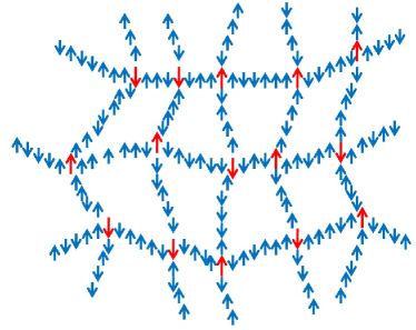
In this figure, the nodal spins, indicated by red color, interact with their four nearest neighbors, which belong to four different chains, while the spins along the one dimensional chains, indicated by blue color, interact with their two nearest neighbors. In this simple network model, a distribution in the number of 1D spins in the chains leads to randomness in the effective interaction between 2D spins.
We will denote the two dimensional spins as where is a two dimensional index running from 1 to where is a very large number. The number, , of spins in the chain connecting sites and dictates the effective “distance” between nodal spins. Selecting the set randomly according to some probability distribution (see below) leads to the realization of a random network of coupled spins. The model Hamiltonian can then be written as:
| (1) |
where and are the 2D and 1D spins respectively. The in the first term on the right are those connected directly to , and the first summation in the last term denotes the sum over all chains, connecting neighboring sites and . The quantity is the exchange energy, which we will set to unity in most of the calculations below. The above formula assumes all . When one of the the corresponding and are connected directly. If all we recover the standard 2D Ising model result with a transition temperature of (we set throughout the paper). When one of the Eq. (1) must be modified so that the term corresponding to the chain connecting and is omitted.
The limit in which all chains are of equal length, , can easily be considered analytically. To do so, we first calculate the partition function for a finite 1D chain. Starting with the Hamiltonian
| (2) |
it is easily shown from elementary transfer matrix methods that the entire system can be mapped onto an ordinary square lattice Ising model, with an effective interaction, , between two four-fold coordinated spins, separated by a “distance” of spins, given by:
| (3) |
The free energy for the coupled Ising model at fixed can then be calculated based on the standard Onsager result, plus an additional contribution from the chains of 1D spins linking the nodal 2D spins. Setting henceforth , the contribution to the free energy from the chains can easily be shown to be (for one chain):
| (4) |
and the contribution from the 2D spins is:
| (5) |
where is defined as:
| (6) |
All thermodynamic quantities can then be calculated from the free energy. We will be interested in the behavior of thermodynamic quantities such as the specific heat and the entropy () since they are important in understanding how the behavior of the system near a phase transition is affected by changes in the dynamics of the network. Other thermodynamic quantities such as the spontaneous magnetization and the magnetic susceptibility can also be studied, but we will focus in this work on the entropy and its derivatives.
In general, we are interested in the case where the vary from chain to chain. Accordingly, we generate a random Ising network by choosing for each chain from a gaussian probability distribution:
| (7) |
where is the average of (average number of 1D spins in a chain) and the standard deviation of the gaussian distribution.
Using this probability distribution, we will investigate, as explained in the Introduction, how the thermodynamic behavior is affected by quenched and annealed disorder in the network. In the quenched case, the value of in each individual 1D chain is fixed but it varies from one chain to the next according to the gaussian random distribution. This serves as a proxy for a disordered network in which the characteristic time scale for changes in the network is much longer than the characteristic time scale for spin fluctuations. For the annealed case, the values of are allowed to thermally fluctuate and this scenario serves as a proxy for a dynamic network whereby the two characteristic time scales mentioned above are comparable to each other. In studying the differences between quenched and annealed disorder, we will focus on features of the heat capacity such as how the temperatures at which has peaks (corresponding to 2D and 1D behavior, see below) change between the two scenarios. Changes in the peak temperatures depending on the type of disorder will allow us to address the question of the role that the dynamics of the network plays in the ordering of the spins.
When one treats the disorder as annealed, the free energy of our system is:
| (8) |
where the angular brackets denote an average over the gaussian probability distribution, Eq. (7). Therefore, needs to be calculated. For a gaussian distribution, this calculation can be done analytically. By tracing over the 1D spins in the chains, the model becomes one in which the 2D spins occupying the nodes interact according to given in Eq. (3). Evaluating then the average of the partition function over the gaussian distribution, the annealed Ising model is mapped onto an effective ferromagnetic square lattice Ising model with equal interactions , given by:
| (9) |
where the average over the discrete gaussian probability distribution indicated by the angular brackets can be easily performed. Thus, the effective interaction for the annealed model is simply a function of and . The annealed free energy can then be calculated based on a procedure similar to the case where is fixed in each link (no disorder) as presented in Eqs. (4-5).
For a system with quenched disorder, the randomness is frozen in each realization of the network. We generate realizations of the network whereby the couplings , satisfying Eq. (3), vary from node to node according to the probability distribution in Eq. (7) for . This corresponds to a model on a regular lattice with a random distribution of couplings . The free energy in the quenched case takes the form:
| (10) |
where the angular brackets still represent an average over the distribution of chain lengths. Since such a calculation is analytically intractable, we use Monte Carlo (MC) simulations to study the thermodynamic behavior of the model with quenched disorder. A standard MC procedure with Metropolis algorithm is used in our study. In each run in the simulation, the heat capacity of the spin system can be obtained either from the fluctuations of the internal energy or by taking the derivative of , (the overbar denote MC averaging) the average energy per spin, with respect to the temperature. By subsequently averaging the heat capacity over a sufficiently large number of realizations of the chain length configurations (over twelve realizations in this study) of , we obtain the heat capacity for the random Ising model with frozen disorder. Each of the 12 realizations is characterized by a unique random set of the effective interaction () between 2D spins.
For the study of any random network, it is important to be able to tune the level of disorder. For the current model, the randomness of the network can be controlled by adjusting the values of and , with the limit recovering the fixed coupled Ising model discussed above. Since the number of 1D spins in the chains cannot be negative, we use values of and such that . With this choice, there is only a very small probability of obtaining negative values for . In such rare cases, in the MC simulation, we set the number of 1D spins in those chains to be two.
The quantity can be used as a measure of the amount of disorder present in the network. A convenient and more physical alternative way to characterize the disorder in this random coupled field model, is via the standard deviation of . Thus, we define a parameter
| (11) |
The quantity (which depends also on ) quantifies the level of disorder in the random Ising model in terms of the spread in the effective interaction between 2D spins. The differences between the properties of quenched and annealed networks can be analyzed in terms of either or with a wide range of values considered for both and .
III Results
In this section we present the results of our study on the random Ising model. We start by briefly discussing the fixed model (, i.e. no disorder) and then proceed to the random model with . For the random model, we analyze differences between quenched and annealed disorder for both components of the coupled field - 1D and 2D - by studying the behavior of the heat capacity and entropy. For the numerical (quenched) results, we have simulated samples with the number of 2D spins () from to , with periodic boundary conditions. Even though the values of used in our simulation are relatively small, the total number of spins, including the 1D ones is much larger: for e.g. a sample network with and the number of spins is approximately Finite size effects in the numerical simulation are also analyzed in order to estimate the error margin associated with our results. These are indicated by error bars where warranted.
III.1 No Disorder
For fixed , the energy and heat capacity can be calculated analytically starting from the free energy expressions in the previous Section, Eqs. (4)-(5). Typical results for the temperature dependence of the energy and heat capacity per spin are plotted in Fig. 2. Since, when considering the disordered () case below we will have to take recourse, in part, to numerical methods, we have also computed the same quantities numerically, to test the same numerical procedures that will be employed later. These results are also plotted in Fig. 2. As mentioned above, the units of temperature throughout this discussion are such that . The numerical results shown there are based on obtaining the average over a sufficiently large number of MC steps per spin: typically about 16,000 turn out to be needed, and then numerically taking the derivative of this average with respect to temperature to obtain the heat capacity. Despite the modest size of chosen for this display, it is clear that the numerical results agree sufficiently well with the analytic results, thereby validating our numerical procedures.
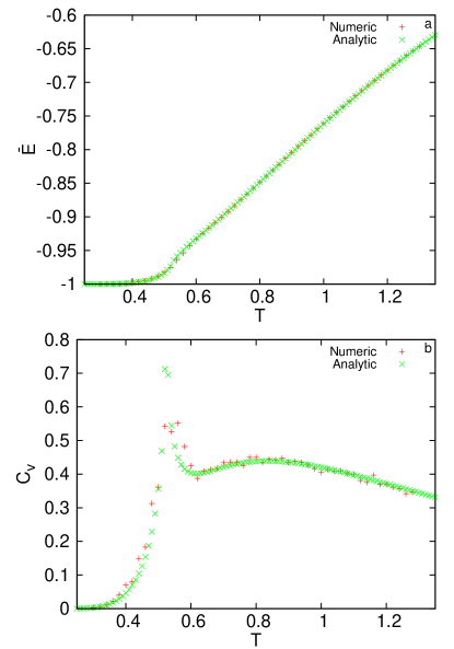
In the heat capacity, features associated with both 2D and 1D spin fields can be seen - the sharp peak in at is associated with the 2D spin field (and the peak position will be henceforth referred to as ) while the broad feature in the heat capacity above is associated with the 1D spin field. The heat capacity eventually approaches zero at higher temperatures.
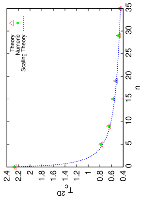
For this case, we should recover the standard 2D Ising model results with an effective interaction and this provides an additional check. Thus, in Fig. 3, we plot vs based on both the analytic calculation (that is, on the Onsager result for ) and the numerical simulation. Again, the numerical results agree with theory. At we recover the well known 2D Ising model transition temperature value, as expected. As increases, decreases indicating that ordering occurs at lower temperatures as the effective coupling between 2D spins decreases or, viewing it in a different way, as the 1D part of the coupled fields becomes more prominent. The relation between and can also be obtained (as an alternative to the calculation) via a simple scaling argument: the ratio of (the number of 1D links between the nodal spins in the network) to the 1D Ising correlation length - (at )- should remain a constant for all at the 2D critical temperature. From this scaling argument, we obtain the following relation:
| (12) |
where is the 2D transition temperature at . This result is plotted as the continuous curve in Fig. 3.
While comparing the analytic results (which are in the thermodynamic limit) to the numerical ones, for , as in Fig. 3, finite size corrections are inevitably present. It is shown in Ref. fisher, that for a 2D Ising model, the difference in between a finite size system ( for a finite system is defined to be the temperature at which the heat capacity peaks) and one in the thermodynamic limit is always positive and given by:
| (13) |
where , and are the critical temperatures for an 2D Ising model and in the thermodynamic limit respectively. For the random coupled field model, the result above is modified due to the presence of 1D spins. The modification to Eq. (13) due to can be calculated by rewriting the equation above in terms of the network model with effective interaction given in Eq. (3):
| (14) |
where denotes , with being the 2D transition temperature for an system with spins in each link. It then follows that:
| (15) |
where and are the 2D transition temperature and effective interaction in the thermodynamic limit. The dependence in the equation above also enters through the effective interaction . The finite size corrections to obtained for our numerical model agree well with the prediction in Eq. (15) above.
III.2 Disorder
After having validated our procedures through the fixed version of our model, we now turn to the random coupled field case. We tune the level of disorder in the random network by adjusting the values and of the gaussian distribution, Eq. (7). Larger values of imply a broader gaussian distribution. As mentioned above, a useful approach to characterize the level of disorder in terms of the effective interaction between 2D spins is the parameter as defined in Eq. (11). Since the effective interaction between the 2D spins depends on , randomness in is reflected on as well. In Fig. 4, we present a plot of vs . The parameter which is simply the standard deviation of the effective interaction between 2D spins, increases with as would be expected, and it is roughly proportional to it. Note that is also temperature dependent. This dependence is weak: in Fig. 4 we have set the temperature to the average annealed value of for each .
III.2.1 Results for 1D fluctuations
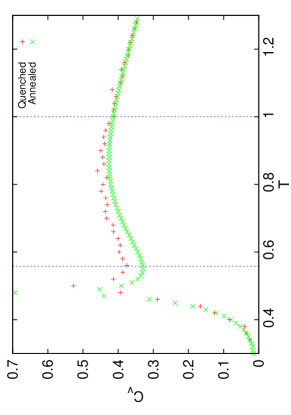
In quantifying differences between quenched and annealed disorder we first look at the 1D field. In each case, we calculate the entropy associated with the 1D fluctuations () from:
| (16) |
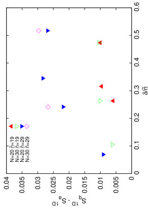
where the temperature limits and are set, in order to take into account the 1D contribution to the total heat capacity, as follows: the lower limit is that of the minimum occurring between the sharp 2D peak and the broad 1D peak (see Fig. 5), while the upper limit is taken to be sufficiently high so that there is no longer any difference between the quenched and annealed specific heats (one may therefore think of as being infinite). In Fig. 6, we plot this difference in the entropies for the quenched and annealed systems, associated with 1D fluctuations, for several values of , and . The weak dependence on is due to finite size effects in the numerical calculation for quenched disorder. The variation with illustrates the actual dependence of this difference on the disorder. We observe that the quenched entropy is always greater than, , the annealed entropy.As the level of disorder in the 1D chains in the network increases, the entropy difference between the quenched and annealed cases increases and then saturates at .
The heat capacity due to the 1D chains alone (in the absence of any 2D spins) can be calculated analytically for both quenched and annealed disorder from Eq. (4) and the rest of the discussion in Sec. II. The temperature dependence of this 1D heat capacity, evaluated for both types of disorder, is shown in Fig. 7.
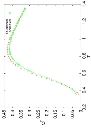
For the example plotted there we see that beginning at , the quenched disorder heat capacity takes on a higher value than the annealed disorder heat capacity. This mostly accounts for the difference in the 1D contribution to the entropy of the coupled system, as evaluated above from Eq. (16) and plotted in Fig. 6.
III.2.2 Results for 2D fluctuations
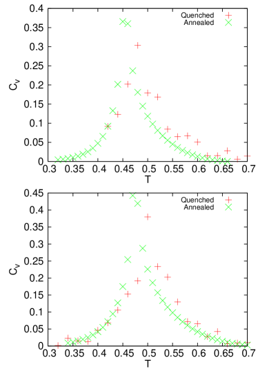
We concentrate here on the differences between quenched and annealed heat capacity due to 2D fluctuations. Since the chain contribution to the heat capacity can be calculated analytically for both quenched and annealed disorder (see discussion in connection with Fig. 7), we isolate the 2D contribution to the specific heat by substracting the chain contribution from the total heat capacity. The total is evaluated analytically in the annealed case and numerically for quenched disorder. The heat capacity due to 2D fluctuations, as obtained in this manner, is shown in the two panels of Fig. 8, which correspond to two different sets of values of and . We see that the results differ for quenched and annealed disorder. An important feature of this difference is that the 2D transition temperature () for a frozen (quenched) random network is always higher than that obtained for the annealed network. In the context of our random network of Ising spins, these results imply that magnetic ordering always takes place at higher temperatures for frozen disorder than if the disorder is allowed to anneal. In other words, as the time scale associated with the dynamics of the network on which Ising spins reside changes from being much larger than the time scale of spin fluctuations (quenched disorder) to a scenario whereby the two time scales are comparable (annealed disorder), the phase transition of the spin system is suppressed. In terms of the dislocation network problem described in the Introduction, our results based on a simplified Ising model suggest that as the dynamics of the dislocation network become important (i.e. when motion of dislocation line segments takes place over time scales comparable to those of fluctuations in the superfluid field), the associated phase transition (in this case superfluid ordering) would be suppressed. Even though superfluid ordering is described by the ferromagnetic XY model, the simplified Ising model we have considered captures the underlying physical principle: the additional fluctuations present in the annealed case will lower the transition temperature.
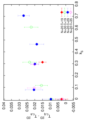
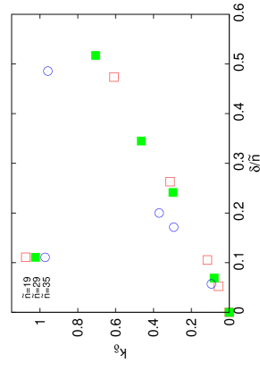
In Fig. 9, we plot the difference in between networks with quenched and annealed disorder. The error bars arise solely from numerical uncertainties in the (quenched disorder) numerical results: for each point in Fig. (9), the quenched 2D transition temperature, , was obtained by averaging over twelve realizations of in the 1D chains in the network. The error bar associated with each data point is the standard deviation of the difference in . It turns out to be more illuminating to plot the results for this difference in terms of the parameter (see Eq. (11)) which characterizes the width of the distribution of effective couplings, rather than in terms of the gaussian width, , and average , of the distribution of . At we recover the ordered results: the difference would be zero in the thermodynamic limit and the small nonzero results arise from finite size effects in the numerical calculation: they are described by Eq. (15). The uncertainties due to finite size effects at higher values of remain the same as in the limit. Earlier studies thorpe ; falk ; thorpe1 on the difference between annealed and quenched disorder, consider the case where the distribution of spin interaction strengths is narrow, and speculate (without any explicit quenched results) that the difference between transition temperatures is small in that limit. Unlike these earlier studies, our model takes into account a broad distribution of effective interaction strengths and we obtain explicitly transition temperatures for both quenched and annealed models. Our results, as seen in the region where (corresponding to a narrow distribution of interaction strengths) of Fig. (9), show that difference in transition temperature is small in this limit. However, we find that as the level of disorder increases, i.e. for higher values of , the difference in between the quenched and annealed networks increases rapidly, until it saturates at . Beyond this value of all the points, regardless of the varying values of and which were used in the calculation, lie within a narrow band of values. Thus, it seems indeed that is sufficient to characterize the phenomena associated with 2D fluctuations, rather than and separately. Interpreting this result in the physical context of a network of dislocation lines, an increase in reflects an increase in the randomness of a network of dislocation lines due to increasing fluctuation in dislocation line lengths making up the network. Our results suggest that, as the randomness in the network increases, the role of the difference in network dynamics (quenched vs annealed) becomes more important.
IV conclusions
In this paper, we have studied the role that the type of disorder - quenched or annealed - plays in the thermodynamic behavior of an Ising model defined on a random network. This network consists of four-fold coordinated Ising spins connected by spin chains. The strength of the disorder can be tuned by varying the average value of the chain length and its standard deviation. We have emphasized both the transition temperature and the specific heat in the region dominated by one dimensional fluctuations. We have shown that the transition temperature for our Ising model on a random network in which the disorder is quenched (frozen) is always higher than the transition temperature for annealed disorder with the same distribution. The magnitude of the difference between the two transition temperatures is quantified by our study. We also show that the entropy associated with the one dimensional fluctuations is larger for the quenched case.
Our study quantifies the difference between the properties of quenched and annealed versions of disordered systems. The quenched assumption applies when the time scale over which the disorder changes is much longer than that for the spin fluctuations. In our model the strength of the effective interaction between neighboring sites has a very broad distribution. Its general interest is that it relates to a variety of experimentally studied systems in which the strength of the effective interaction between neighboring spins has a very broad distribution. An example is dilute magnetic semiconductors. Our results indicate that the transition temperature and other thermodynamic properties of dilute magnetic semiconductors might be approximated from an analytic calculation for the annealed model with the same distribution of interaction strengths. Our model may be relevant also to the renewed interest on dislocation networks in solid 4He. It presents a simplified version of how the dynamics of a dislocation network may influence a superfluid field in its vicinity. Our results indicate that in the annealed scenario, when fluctuations of dislocation line segments within a network become important i.e. when the time scale for dislocation line fluctuations becomes comparable to or smaller than the time scale associated with fluctuations of the superfluid field, the associated phase transition is suppressed. On the other hand, superfluid ordering would be enhanced in the vicinity of a dislocation if the dislocation network can be considered to be frozen. While our results have been obtained for a simplified Ising version of the superfluid transition, we expect that the general conclusion about the transition being suppressed by fluctuations in the dislocation network will remain valid when the proper symmetry of the superfluid order parameter (XY model) is taken into account. Quantum effects, considered in Ref. balibar, , but not taken into account in our study, are expected to enhance the suppression of the superfluid transition by the motion of dislocation lines.
Acknowledgements.
This research was supported in part by IUSSTF grant 94-2010. A.M.K. would like to thank Sumanta Bandyopadhyay and Cole Grasse for their help.References
- (1) T.C. Lubensky, in Ill Condensed Matter, Les Houches Session XXXI, Edited by R Balian, R Maynard and G Toulouse (North Holland, Amsterdam, 1979).
- (2) R.B. Stinchcombe, in Phase Transitions and Critical Phenomena Vol. 7, edited by C. Domb and J.L. Lebowitz (Academic, New York, 1983).
- (3) D. Stauffer and A. Aharony, Introduction to Percolation Theory, 2nd edition (Taylor and Francis, Philadelphia, 1994).
- (4) A. S. Skal and B. I. Shklovskii, Fiz. Tekh. Poluprovodn. 8, 1582 (1974) [Sov. Phys.-Semicond. 8, 1029 (1975)].
- (5) C. Dasgupta, A. B. Harris, and T. C. Lubensky, Phys. Rev. B 17, 1375 (1978).
- (6) Y. Gefen, A. Aharony and B.B. Mandelbrot, J. Phys. A 17, 435 (1984).
- (7) R.B. Stinchcombe, Phys. Rev. B 41, 2510 (1990)
- (8) R. Albert and A.-L. Barabasi, Rev. Mod. Phys. 74, 47 (2002).
- (9) S. N. Dorogovtsev and J. F. F. Mendes, Adv. Phys. 51, 1079 (2002).
- (10) S. N. Dorogovtsev and J. F. F. Mendes, Evolution of Networks: From Biological Nets to the Internet and WWW (Oxford University Press, Oxford, 2003).
- (11) G. Fagiolo and M. Mastrorillo. Phys. Rev. E 88, 012812 (2013).
- (12) M. Boguna, C. Castellano, R. Pastor-Satorras. Phys. Rev. Lett. 111, 068701 (2013).
- (13) D.J.Watts and S.H.Strogatz, Nature (London) 393,440 (1998).
- (14) A.-L.Barabasi and R. Albert, Science 286, 509 (1999).
- (15) A. Majdandzic, B. Podobnik, S.V. Buldyrev, D.Y. Kenett, S. Havlin and H.E. Stanley. Nature Physics 10, 34-38 (2014).
- (16) A. V. Goltsev, S. N. Dorogovtsev, and J. F. F. Mendes, Phys. Rev. E 67, 026123 (2003).
- (17) S. N. Dorogovtsev, A. V. Goltsev and J. F. F. Mendes, Phys. Rev. E 66, 016104 (2002).
- (18) M. Leone, A. Vazquez, A. Vespignani, R. Zecchina, Eur. Phys. J. B 28, 191 (2002).
- (19) C. P. Herrero, Phys. Rev. E 77, 041102 (2008).
- (20) D.-H. Kim, G. J. Rodgers, B. Kahng, and D. Kim, Phys. Rev. E 71, 056115 (2005).
- (21) T. Hasegawa and K. Nemoto. Phys. Rev. E 80, 026126 (2009).
- (22) F. Igloi and L. Turban, Phys. Rev. E 66, 036140 (2002).
- (23) S. N. Dorogovtsev, A. V. Goltsev, and J. F. F. Mendes, Eur. Phys. J. B 38, 177 (2004).
- (24) B. J. Kim, H. Hong, P. Holme, G. S. Jeon, P. Minnhagen, and M. Y. Choi, Phys. Rev. E 64, 056135.
- (25) M.I. Berganza and L. Leuzzi, Phys. Rev. B 88, 144104 (2013).
- (26) F.W.S Lima and J.A. Plascak, J. Phys.: Conf. Ser. 487, 012011 (2014).
- (27) R.F.S. Andrade, J.S. Andrade Jr. and H.J. Herrmann, Phys. Rev. E 79, 036105 (2009).
- (28) M. Serva, U. L. Fulco and E. L. Albuquerque, Phys. Rev. E 88, 042823 (2013).
- (29) A. B. Harris, J. Phys. C 7, 1671 (1974).
- (30) M. E. Fisher, Phys. Rev. 176, 257 (1968).
- (31) M.F. Thorpe and D. Beeman, Phys. Rev. B 14, 188 (1976).
- (32) H. Falk, J. Phys. C: Solid State Phys., 9, L213 (1976).
- (33) M.F. Thorpe, J. Phys. C: Solid State Phys., 11, 2983 (1978).
- (34) S. Balibar and F. Caupin, J. Phys. Condens. Matter 20, 17320 (2008).
- (35) L. Pollet, M. Boninsegni, A.B. Kuklov, N.V. Prokof’ev, B.V. Svistunov and M. Troyer, Phys. Rev. Lett. 98, 135301 (2007).
- (36) M. Boninsegni, A.B. Kuklov, L. Pollet, N.V. Prokof’ev, B.V. Svistunov and M. Troyer, Phys. Rev. Lett. 99, 034301 (2007).
- (37) S.I. Shevchenko, Fiz. Nauk. Temp. 14 (1988) [Sov. J. Low Temp. Phys 14, 553 (1988)].
- (38) A.T. Dorsey, P. M. Goldbart, and J. Toner, Phys. Rev. Lett. 96, 055301 (2006).
- (39) J. Toner, Phys. Rev. Lett. 100, 35302 (2008).
- (40) C. Dasgupta and O.T. Valls, Phys. Rev. B 82, 024523 (2010).
- (41) S. Balibar, Nature (London) 464, 08913 (2010); Physics 3, 39 (2010).
- (42) E. Kim and M.W.H. Chan, Science 305, 1941 (2004).
- (43) D. Kim and M. Chan, Phys. Rev. Lett.109, 155301 (2012).
- (44) V.M. Galitski, A. Kaminski, and S. Das Sarma, Phys. Rev. Lett. 92, 177203 (2004).
- (45) A. Kaminski and S. Das Sarma, Phys. Rev. Lett. 88, 247202 (2002).
- (46) I. Ya. Korenblit, E. F. Shender and B. I. Shklovskii, Phys. Lett. A 46, 275 (1973).
- (47) R. N. Bhatt and P. A. Lee, Phys. Rev. Lett. 48, 344 (1982).
- (48) D. Aleinikava, E. Dedits, A.B. Kuklov and D. Schmeltzer, Europhys. Lett. 89, 46002 (2010).
- (49) A.E. Ferdinand and M.E. Fisher. Phys. Rev. Lett. 185, 2 (1969).