Surface layer independent model fitting by phase matching:
theory and application to HD49933 and HD177153 (aka Perky)
Abstract
Aims. To describe the theory of surface layer independent model fitting by phase matching and to apply this to the stars HD49933 observed by CoRoT, and HD177153 (aka Perky), observed by Kepler
Methods. We use theoretical analysis, phase shifts, and model fitting.
Results. We define the inner and outer phase shifts of a frequency set of a model star and show that the outer phase shifts are (almost) independent of degree , and that a function of the inner phase shifts (the phase function) collapses to an independent function of frequency in the outer layers. We then show how to use this result in a model fitting technique to find a best fit model to an observed frequency set by calculating the inner phase shifts of a model using the observed frequencies and determining the extent to which the phase function collapses to a single function of frequency in the outer layers. We give two examples applying this technique to the frequency sets of HD49933 observed by CoRoT and HD177153 (aka Perky) observed by Kepler, and compare our results with those of previous studies and show that they are compatible with those obtained using different techniques. We show that there can be many different models that fit the data within the errors and that better precision on the frequencies is needed to discriminate between the models. We compare this technique to that using the ratios of small to large separations, showing that in principle it is more accurate and avoids the problem of correlated errors in separation ratio fitting.
Key Words.:
stars: oscillations, - asteroseismology - stars: interiors - methods: analytical - methods: numerical1 Introduction
At first sight, the obvious way to seek to infer the internal structure of a star with an observed frequency set , with error estimated is to search for a model (or models) whose frequencies fit the observed values within the error estimates. However it has long been appreciated that this is not so straight forward: modelling of the outer layers of a star is subject to considerable uncertainties (cf Christensen-Dalsgaard et al, 1988, Dziembowski et al 1988) due to our poor understanding of the physical processes that determine the structure of these layers; these include modelling convection, convective overshooting, non-adiabatic effects on both convection and oscillations, turbulent pressure, the equation of state, diffusion, mild turbulence, magnetic fields, rotation and global circulation. All these factors impact on the oscillation frequencies of a model star, and therefore hinder efforts to find stellar models whose frequencies best fit an observed frequency set. Even for the solar case observations and models disagree by up to Hz.
One way of seeking to overcome these problems is the “frequency offset technique” (Kjeldsen et al 2008), in which the difference between the observed solar frequencies and those of a “best solar model” is fitted by a power law , which is then scaled by a single factor (determined by the average frequency and large separation) and applied to other stars when seeking a best fit model. This technique is widely used and has been incorporated into the Asteroseismic Modeling Portal (AMP) software (Metcalfe et al 2009). However the assumption that the many differences in the properties of the outer layers of different stars can be captured in a single scaling factor remains to be verified.
A second method is fitting separation ratios: that is finding models whose frequencies are such that their ratios of small to large separations best fit the same ratios of the observed frequency set, since such ratios subtract off the major effects of the outer layers (Roxburgh and Vorontsov 2003). But note that, as pointed out in Roxburgh and Vorontsov (2013), it is not the ratios at the same values that should be compared but rather the model values interpolated to the observed frequencies. Note also that since the ratios only depend on the structure of the inner layers, they can only give information on the interior of a star and not on the outer layers.
We here present an alternative surface layer independent procedure (Phase Matching) that rests on the result that in the outer layers of a star the phase shift of the eigenfunction of an oscillation mode (that is the departure from a pure harmonic function) is almost independent of the angular degree , so that even though we do not know what is, for the model to fit the frequencies a function (the phase function) of the inner phase shifts , calculated at the observed frequencies, must be such that it matches on to a function only of frequency in the outer layers.
Details of the analysis are given in section 2, illustrated using models of a star in different stages of evolution, primarily Model A (mid main sequence); Model B (terminal main sequence) and Model C (post main sequence in the shell burning phase). In section 3 this procedure is applied to the frequency sets of the CoRoT star HD49933 and the Kepler star HD177153 (aka Perky) to find best fit models, and the results compared with those obtained by other authors: Piau et al (2009), Benomar et al (2010), Kallinger et al (2010), Bigot et al (2011), Creevey and Bazot (2011) and Liu et al (2014), Silva-Aguire et al, (2013). In section 4 we compare the method to that using separation ratios, showing that it is in principle more accurate and that it avoids the problem of correlated errors when using separation ratios.
2 Theory of model fitting by phase matching
2.1 The phase shifts
For any angular degree the frequencies of a model star are given as the eigenvalues of the 4th order system of equations governing the oscillations, but for radial () modes the equations reduce to 2nd order in the variable
is the acoustic radius, the Eulerian pressure perturbation, , and and are acoustic potentials that depend on both frequency and the structure variables: density , pressure , sound speed () and adiabatic exponent . Were and , this is just the simple harmonic equation whose solution is .
Since Eqn 1 is a 2nd order homogeneous equation it can be reduced to a 1st order inhomogeneous equation in the variable and solved in terms of an inner phase shift defined by
where satisfies the equation
The central boundary condition of regularity at requires at 111or for integer ; given the structure of the star can be evaluated at any for any (not necessarily an eigenvalue), and the value at any is determined solely by the structure interior to . Of course in general Eqn 2 does not satisfy the surface boundary condition on , the requirement that it do so determines the eigenfrequencies.
One can equally write Eqn 1 in terms of the acoustic depth where is the total acoustic radius of the star and represent the solution in the form
where satisfies the surface boundary conditions on the gravitational potential and pressure perturbation 222again subject to the addition of any multiple of . For modes the gravitational boundary condition that the potential and its derivative are continuous with a solution of Laplace’s equation is automatically satisfied (by conservation of mass and Newton’s sphere theorem), and is a continuous function of and , determined solely by the structure of the outer layers above .
For an eigenfrequency must be continuous at all , hence on equating the expressions in Eqns (2) and (4) at any intermediate , and recalling that if then for integer , and that , we obtain the result that an eigenfrequency satisfies 333this absorbs the arbitrary in the boundary conditions
where is the total acoustic radius.
For we replace Eqns 2 and 4 by
Eqn 6a reflects the fact that the eigenfunctions behave like spherical Bessel functions near . Eqn 5 becomes
This is the Eigenfrequency Equation of Roxburgh and Vorontsov (2000, 2003). Note that here is an unknown integer, it may be related to the radial order, as is the case for p-modes in main sequence stars, but it loses any such meaning in more evolved stars which have mixed modes.
For the equations can again be reduced to 2nd order (Takata 2005, Roxburgh 2006, 2008a) so, for any , is a continuous function of and a continuous function of (the surface condition on the gravitational potential being automatically satisfied by momentum conservation and MacCullagh’s (1855) theorem).
For the equations remain of 4th order. One can readily determine and from Eqns 6a and 6b for eigenfrequencies , but one can also determine for any , applying the gravitational boundary condition, but not the pressure condition, at the surface or anywhere in the outer layers where the density is negligible. One can also determine a continuous by the (very good) approximation of setting the oscillating gravitational potential and its derivative to zero at the surface. (These approximations are discussed in the Appendix) Alternatively for main sequence stars one can reduce the 4th order system of equations to second order by using the short wavelength Born approximation (Roxburgh and Vorontsov 1994a).
The conclusion of this section is that given a stellar model we can determine continuous inner phase shifts for any frequency at any acoustic radius in the outer layers of a star determined solely by the structure of the star interior to , and continuous outer phase shifts that are determined solely by the structure of the outer layers above .
2.2 The phase function: a main sequence example
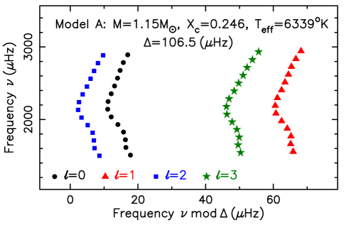
To illustrate the analysis we consider Model A, a model of a star of mass with initial hydrogen abundance , heavy element abundance , evolved to a central hydrogen abundance , at an age of ys. The model frequency set is shown in the echelle diagram in Fig 1, and has 14 frequencies in the range Hz for each . The mean large separation Hz.
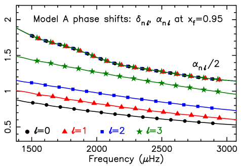
In Fig 2 we show these phase shifts for Model A evaluated at a fractional radius . The depend on both degree and radial order , whereas the almost all lie on the same curve independent of degree , the maximum departure (see Appendix). It is this independence that is the basis of the phase matching technique (and of the use of separation ratios). The curves in his figure are the continuous phase shifts calculated as described in the previous section.
The acoustic radius is not an observable, so we write Eqn 7 in terms of the observable mean large separation (eg the value Hz in Fig 1) and a phase function defined by
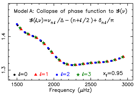
Taking to be an independent function of , and the last term just a linear function of , it follows that is independent of . This is shown in Fig 3 for our model star. With an assumed error on the frequencies of Hz the reduced for a fit to a function only of at is , and is smaller if is taken closer to the surface since decreases with increasing (see Appendix).
This result provides the basis of model fitting by phase matching. If the model star has the same interior structure as an observed star then the function of the internal phase shifts of the model calculated using the observed frequencies should collapse to a single function of frequency. The extent to which this is satisfied is a measure of the goodness of fit.
2.3 Mixed modes
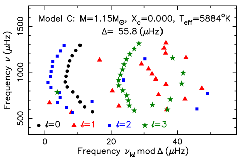
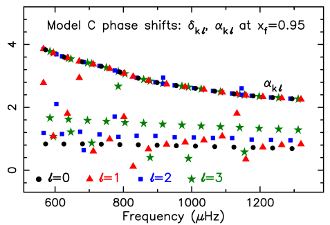
The above is all for p-modes where the frequencies all follow a regular pattern and the value is related to the radial order of a mode - essentially the number of nodes in the eigenfunction. But for later stages of evolution where there are mixed modes the situation is more complicated. We give an example of such a star, Model C, which is well beyond the main sequence and into the hydrogen shell burning phase as the star moves over to the red-giant branch in the H-R diagram. The echelle diagram for frequencies in the range Hz is shown in Fig 4, there are many mixed modes. The subscript is here just a label to distinguish different frequencies as .
One can of course still calculate the inner and outer phase shifts, of the and the they still necessarily satisfy Eqn 7, with some integer. The phase shifts are shown in Fig 5 . As the phase shifts are are only determined to within a multiple of we have added or subtracted an integral number of to bring all the inner phase shifts within the interval }. The outer phase shifts still lie on a single curve .
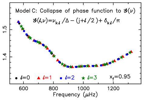
To calculate the phase function we define the integer by
and the phase function by
The resulting is shown in Fig 6. It collapses to a single function of frequency.
2.4 Model fitting by phase matching
We here summarise the phase match algorithm.
Given a set of observed frequencies with error estimates , and a model to be tested for goodness of fit, determine the inner phase shifts of the model at the observed frequencies (Eqn 6a) and hence the phase function for that model (Eqn 8), where is any estimate of the average large separation of the .
Repeat this calculation for frequencies and subtract to determine error estimates on the determination of .
Then determine , a best fit function of frequency to the with errors ( being the number of parameters in ), and determine the goodness of fit in terms of
where N is the number of frequencies. In practice is modelled as a series in Chebyshev polynomials and is taken to minimise , where is the number of frequencies.
All models with have an interior structure that is consistent with the observed frequencies.. Surface layer independent model fitting algorithms necessarily cannot give information on the outer layers of the star.
To determine the for any and , one obtains the solution of the oscillation equations for this and which satisfy the the boundary condition of regularity at , and the surface boundary condition that the gravitational potential perturbation and its derivative are continuous with a solution of Laplace’s equation, . In general this consists of calculating the two independent solutions from the centre and combining them to satisfy the Laplace condition; this can be done at any point in the outer layers since these low density regions make a negligible contribution to . One then forms the scaled Eulerian pressure perturbation and its derivative at some point (eg where ). The inner phase shifts can then be determined (for example) by
where
We emphasise that the surface phase shift of the model does not enter into this algorithm, all that is assumed is that the unknown surface phase shift can be modelled by a single function of frequency.
One may of course add other restrictions on the models: mass, luminosity, radius, effective temperature, surface gravity, surface composition …but these are not tested by surface layer independent model fitting,
2.5 An example
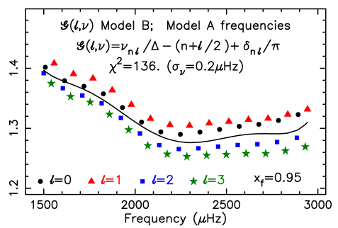
To demonstrate the phase matching technique we take the frequencies of Model A as the observed frequencies , with an assumed error estimate Hz on all frequencies, and test for a fit to other models in the same evolutionary sequence. The first example is Model B, the model evolved to a central hydrogen abundance of at an age of ys.
The results are shown in Fig7 ; does not collapse to a function only of , The continuous curve is the least squares fit to a single function of , the error estimates on are too small to be seen in this figure. The of the fit is ; the observed frequencies of model A do not fit model B.

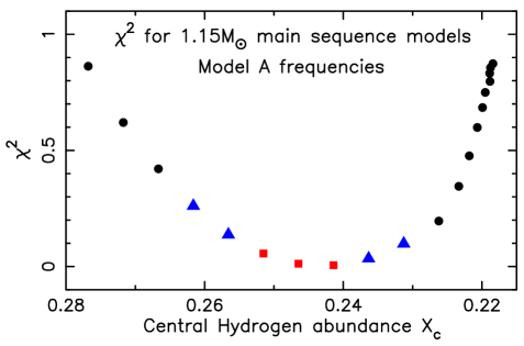
We then repeated this analysis for a set of models in the evolutionary sequence of the star from the initial main sequence , to terminal main sequence with at an age of ys. Fig 8 shows the resulting for this series of models. Obviously models that are far removed from Model A have a very poor fit, so to examine more closely the models in the neighbourhood of ModelA we used a finer output mesh in the evolutionary calculation and the models with are shown in Fig 9. With an estimated error on the frequencies of Hz all these models fit the observed input frequencies..
To further restrict the models we need to impose additional constraints. As pointed out in Roxburgh (2014), since the objective of surface layer independent model fitting is to subtract out the effect of the outer layers it is inconsistent to impose a constraint that the model large separation fits the observed value since the outer layers of a star make a major contribution to the large separations. To a lesser extent the same is true of the radius, but the luminosity of the star is determined solely by the interior structure so it is reasonable to require the the model luminosity fits the observed value - in this case the luminosity of Model A.
For an increasing number of stars bolometric flux measurements and parallaxes give the luminosity to high precision, often better that ( cf Boyajian et al, 2013). In Fig 9 the red squares match the luminosity of ModelA to within whilst the blue triangles match to within - much restricting the models that fit the input model.
3 Application to HD 49933 and HD 177513
3.1 Constraints on model fitting
Since the objective of phase matching model fitting (and model fitting using the ratios of small to large separations) is to subtract off the unknown effect of the outer layers of a star and find the best interior model, it would be inconsistent to constrain the model search by observed parameters that depend on the structure of the outer layers. The two truly outer layer independent constraints are the mass and luminosity . The luminosity can be estimated using the parallax and either the magnitude or measurements of the bolometric flux. The mass may be dynamically determined for stars in a binary system (eg Cen A&B), or from the radius (determined either by interferometry or from and spectroscopically determined ) combined with a spectroscopically determined surface gravity . The atmospheric composition is clearly a surface layer parameter. The outer layers make a large contribution to the large separation (Roxburgh 2014) and a smaller contribution to the radius, so estimating mass from the (approximate) scaling relation for the large separation should be treated with caution. Ideally therefore we should constrain our model search just imposing constraints on the mass and luminosity; the radius can be used whilst recognising that it is also subject to some uncertainty due to uncertainty in the structure of the outer layers. Were we to find in our model fitting by phase matching, constrained solely by the estimates of , that a best fit model also fitted the observed radius, large separation and surface composition this would be a bonus - indicating that our modelling of the outer layers is reasonable. But a model that best fits the interior may not fit the outer layer constraints because the modelling of the outer layers is incorrect.
3.2 HD49933
The star HD 49933 was observed by CoRoT in 2 separate runs; the initial short run was described in Appourchaux et al (2008) and the combined date from the two runs in Benomar et al (2009) who tabulated a total of 50 frequencies in the range Hz including modes of degree . These are the frequencies used in our analysis. There is no unique way of defining the average large separation but if one wishes to compare model and observed values we should at least use the same definition for both. We therefore define as the average over 5 frequencies centred around the frequency closest to Hz, which gives a value Hz, the error estimate allowing for the quasi periodic behaviour of the large separations of HD49933 with frequency (cf Benomar et al 2009) and the difference between the observed solar value and that of solar models.
Taking the parallax from van Leeuwen (2007), angular diameter from Bigot et al (2011), bolometric flux from Boyajian et al (2013) gives K. But it is difficult to put any reliable constraints on the mass. Spectroscopic and photometric measurements of made by several authors are summarised in Bruntt (2009) who gives his most recent values as (spectroscopic) and (photometric). These differ very substantially from the value of from Kallinger et al (2010). If we use Bruntt’s spectroscopic value and Bigot’s radius the range for the mass is . For comparison the mass range from using the scaling relation on is , but the scaling relation itself is, at best, only approximate, so we do not use this as a constraint but directly compare the model and observed s. These parameters are listed in Table 1.
Table 1. HD 49933: Possible constraints on model fitting
We searched for a best fit model using only the phase match criterion plus the luminosity constraint. The model set was constructed using the STAROX code (Roxburgh 2008b) which has GN93 relative abundances (Grevesse and Noels 1993), OPAL opacities (Iglesias and Rogers 1996) supplemented by Whichita opacities at low temperatures (Ferguson et al 2005), and NACRE reaction rates (Angulo et al 1999) (taking 13C, 15N and 17F to be in equilibrium), the mixing length model of convection (with mixing length=), two models of convective overshoot and mixing from a convective core, one set (IR1) with just chemical mixing a distance of , the second (IR2) with full entropy and chemical mixing a distance where is the distance given by the Integral Constraint (Roxburgh 1978, 1989). These models do not include diffusion so we also search a model set (AM) kindly supplied by A Miglio (2012) computed using the Liège CLÉS code (Scuflaire et al 2008) with and without chemical overshooting and diffusion. The model set IR1 has 100,440 models with mass , initial composition , , , and . Model set IR2 has models with the same parameter set but
A very large number of models were found to fit the both the phase match and luminosity constraints to within a ; from set IR1, and from IR2, with masses ranging from and ages from ys, all with some core overshooting. Imposing the mass constraint reduces this slightly to and , restricting the mass range to . Imposing the radius constrain reduces this to for IR1 and for IR2 but still with a similar range in mass and age. Finally imposing the large separation constraint reduces the models to 7 from IR1, 2 from IR2 and 4 from AM: details of these models are given in Table 2. Figure 10 shows the phase match function for one of the IR2 models. No models with diffusion and/or no overshooting satisfied all the constraints.
Table 2: Best fit models HD49933: IR1, IR2, AM model sets.
| Set | |||||||||||
| IR1 | 1.26 | 86.2 | 0.39 | 0.61 | |||||||
| IR1 | 1.22 | 85.5 | 0.35 | 0.65 | |||||||
| IR1 | 1.20 | 86.3 | 0.35 | 0.69 | |||||||
| IR1 | 1.22 | 85.3 | 0.30 | 0.80 | |||||||
| IR1 | 1.20 | 84.7 | 0.29 | 0.84 | |||||||
| IR1 | 1.22 | 84.4. | 0.39 | 0.86 | |||||||
| IR1 | 1.22 | 85.4 | 0.29 | 0.88 | |||||||
| IR2 | 1.24 | 85.7 | 0.39 | 0.67 | |||||||
| IR2 | 1.22 | 85.7 | 0.35 | 0.73 | |||||||
| AM | 1.22 | 86.2 | 0.38 | 0.61 | |||||||
| AM | 1.26 | 86.3 | 0.45 | 0.66 | |||||||
| AM | 1.24 | 85.2 | 0.43 | 0.66 | |||||||
| AM | 1.22 | 85.7 | 0.42 | 0.66 | |||||||
| IR1 | 1.10 | 86.3 | 0.29 | 0.80 | |||||||
| AM | 1.30 | 86.6 | 0.52 | 0.81 |
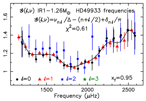
However if we drop the constraint on the mass from and relax the constraint on just a little then we obtain many more models; two examples are given at the end of Table 2 - the AM model includes diffusion.
The obvious conclusion from these results is that the precision on the frequencies is not good enough to determine a best fit model. The wide range of models that fit the data are compatible with the values found by Piau et al (2009), Benomar et al (2010), Kallinger et al (2010), Bigot et al (2011), Creevey and Bazot (2011) and Liu et al (2014).
3.3 HD 177153 (aka Perky)
The star HD 177153 was observed by Kepler (KIC 6106415, aka Perky) and analysed by Silva Aguire et al (2013) who list a total of 33 frequencies in their Table 1, 11 for each ; these are the frequencies used in this analysis. Silva Aguire et al searched for best fit models by two procedures,: comparing frequencies with a ”surface offset” (cf Kjeldsen et al 2008), and comparing separation ratios (cf Roxburgh and Vorontsov 2003, 2013) - in fact a subset of ratios (but see comments below). Here we seek best fit models by phase matching. and compare our results with theirs.
These authors also list global parameters which we reproduce in Table 3 and use in our analysis, determining the radius constraint from and the mass constraint from the radius and . We determine the large separation from the 5 frequencies centred on Hz, not from the autocorrelation of the time series (cf Roxburgh and Vorontsov 2006) as one cannot compute model values by this technique, and we take an enhanced error estimate on as was done for HD49933.
Table 3. HD 177513 Possible constraints on model fitting
We then searched our model sets to find models that fitted the above constraints, using the full set of 33 frequencies, and for which the phase function collapsed to a function only of within a (Eqn 9). We included the model set IR0 which is the same as IR1 except that it follows the evolution of 13C, 15N and 17F.
Again there are many models (77) that fit the constraints without fitting the large separation, whose value is sensitive to the detailed structure of the outer layers so should not logically be imposed as a constraint on surface layer independent model fitting. If we nevertheless impose this constraint along with that of the luminosity, radius (or effective temperature) and mass (from ) we find 20 models that satisfy these constraints and also the phase match condition; these are listed in Table 4. All best fit models listed have no overshooting: models IR0 have no diffusion; models AM all have diffusion (see Scuflaire 2008). The fit for one such model (IR01 ) is shown in Fig 11.
The models cover a mass range of to with ages in the range to ys. This is very similar to the range of models in Tables and in Silva Aguire et al (2013). which has a mass range and ages varying between to ys, although only 2 of their models have a .
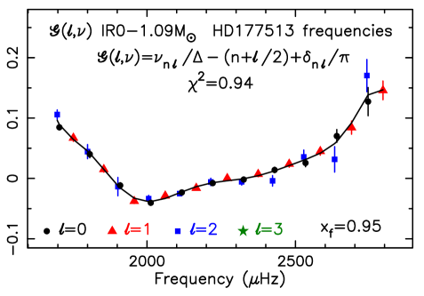
Table 4: Best fit models HD177513: IR0, AM model sets.
| Set | ||||||||||
|---|---|---|---|---|---|---|---|---|---|---|
| IR0 | 1.08 | 1.70 | 1.23 | 0.70 | 0.020 | 1.6 | 4.86 | 104.8 | 0.10 | 1.00 |
| IR0 | 1.09 | 1.70 | 1.24 | 0.70 | 0.021 | 1.6 | 4.80 | 104.5 | 0.10 | 0.94 |
| IR0 | 1.11 | 1.70 | 1.25 | 0.70 | 0.023 | 1.6 | 4.72 | 103.6 | 0.10 | 0.94 |
| IR0 | 1.13 | 1.91 | 1.24 | 0.72 | 0.019 | 1.8 | 4.48 | 105.2 | 0.10 | 1.00 |
| IR0 | 1.11 | 1.69 | 1.24 | 0.72 | 0.020 | 1.6 | 4.86 | 105.2 | 0.15 | 0.96 |
| IR0 | 1.14 | 1.91 | 1.25 | 0.72 | 0.020 | 1.8 | 4.46 | 104.9 | 0.10 | 0.94 |
| IR0 | 1.12 | 1.69 | 1.24 | 0.72 | 0.021 | 1.6 | 4.83 | 104.8 | 0.14 | 0.99 |
| IR0 | 1.15 | 1.90 | 1.25 | 0.72 | 0.021 | 1.8 | 4.42 | 104.8 | 0.10 | 0.93 |
| IR0 | 1.15 | 1.85 | 1.25 | 0.72 | 0.022 | 1.8 | 4.61 | 105.1 | 0.10 | 0.91 |
| IR0 | 1.13 | 1.91 | 1.24 | 0.73 | 0.018 | 1.8 | 4.72 | 105.2 | 0.10 | 0.96 |
| IR0 | 1.14 | 1.90 | 1.25 | 0.73 | 0.019 | 1.8 | 4.70 | 104.9 | 0.10 | 0.90 |
| IR0 | 1.12 | 1.68 | 1.24 | 0.73 | 0.020 | 1.6 | 5.09 | 104.9 | 0.15 | 0.92 |
| IR0 | 1.15 | 1.90 | 1.26 | 0.73 | 0.020 | 1.8 | 4.70 | 104.5 | 0.10 | 0.91 |
| IR0 | 1.13 | 1.68 | 1.25 | 0.73 | 0.021 | 1.6 | 5.08 | 104.5 | 0.15 | 0.98 |
| AM | 1.11 | 1.75 | 1.24 | 0.71 | 0.020 | 1.7 | 4.75 | 104.7 | 0.13 | 0.85 |
| AM | 1.10 | 1.66 | 1.23 | 0.68 | 0.025 | 1.7 | 4.59 | 105.0 | 0.17 | 0.88 |
| AM | 1.13 | 1.86 | 1.25 | 0.68 | 0.025 | 1.9 | 4.21 | 104.8 | 0.20 | 0.88 |
| AM | 1.12 | 1.70 | 1.25 | 0.69 | 0.025 | 1.7 | 4.62 | 103.8 | 0.17 | 0.87 |
| AM | 1.15 | 1.89 | 1.25 | 0.69 | 0.025 | 1.9 | 4.13 | 104.7 | 0.22 | 0.92 |
| AM | 1.14 | 1.73 | 1.26 | 0.70 | 0.025 | 1.7 | 4.53 | 103.8 | 0.18 | 0.97 |
However a difference is that we find many different models that satisfy the constraints, all produced by the same stellar evolution code with the same physical assumptions, in contrast to the range of models in Silva Aguire (2013) which were computed using different stellar evolution codes. There is a lesson in this: if one were to search for a best fit model using some minimisation algorithm, the multi-dimensional surface in which one is seeking a minimum can have many local minima consistent with the data and its error estimates, that is with a . It is not statistically sound to search for the minimum with the lowest value of and consider this to be the ”correct” model; all are consistent with the data. To discriminate between the models one needs data of greater precision.
In their analysis Silva Aguire et al (2013) combined ratios and ratios into a single series and sought models that fit the combined data points. But the are not independent, one set can in principle be obtained from the other by interpolation. Half the frequencies are used in eliminating the surface phase shift so there are only independent data (see next section), taking over estimates the .
4 Relation to separation ratios
Surface layer independent model fitting, phase matching and separation ratios, are both based on the result that in the outer layers of a star the surface phase shift is, to a very good approximation, independent of so that which can be considered a continuous function of (see Appendix).
For any estimate of the average large separation , the oscillation frequencies can always be expressed in terms of functions in the form
where, for any set of frequencies. the functions are known at a discrete set of values
From the Eigenfrequency Equation (Eqns 7,8), can be expressed in terms of the inner and outer phase shifts as
With independent of , the term in square brackets in this equation (which we call ) is a function only of .
The phase match algorithm uses this equation in the form
is a function only of ; the separation ratios algorithm uses it to subtract off the by interpolating in the discrete set of the for values at the same frequencies, and eliminating by subtraction to determine the inner phase shift differences, eg
which only depend on the inner structure of the star. If one uses linear interpolation one readily obtain the result that
where (and its relative ) are the separation ratios.
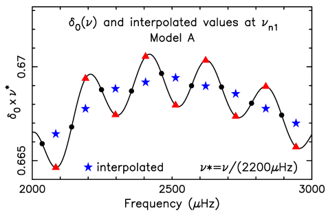
A source of error in the separation ratio technique is the error in interpolation; this can be reduced by using higher order interpolation algorithms, such as the 5 point expressions for , but they still have an error which can be significant if the quasi periodic modulation in the s is on a scale smaller than twice the large separation. In Fig 12 we illustrate this by interpolating for the values of at frequencies from the values at for Model A. The curve is the continuous phase shift , the black points are the discrete phase shift at the frequencies , the red triangles the values at frequencies , and the blue stars the values at determined from the by cubic interpolation.

The quasi periodicity in the s is due to the rapid variation in acoustic variable at the base of a convective envelope, the period being determined by the acoustic radius of the interface and the amplitude by the strength of the quasi discontinuity (Roxburgh (2009). It is only an important source of error if the error from interpolation is larger than that due to errors on the frequencies. This is not the case for Model A, Fig 13 shows the values of the 5 point small separations compared with to actual phase shift difference, the error bars corresponding to an error of Hz on the frequencies.
We note here that one can interpolate for the value of and at any and, on subtraction, obtain an approximation to the the phase shift difference at any , but this does not increase the number of independent variables. If one has values of each of and , then essentially of them are used to model leaving independent data on . This is why it is incorrect to add together the series of ratios and and consider this as data.
The phase matching technique requires that the unknown outer phase shifts can be well approximated by a polynomial in determined by the all the inner phase shifts of the total number of observed frequencies. The outer phase shifts also have a quasi-periodicity determined primarily by the acoustic depth of the HeII ionisation zone, but this period is typically many large separations and so can be accurately modelled by a polynomial in . A further advantage of the phase match technique is that in the fitting process the errors are uncorrelated, whereas in the separation ratios technique the errors on the ratios are strongly correlated.
Appendix
Accuracy of the approximation
Surface layer independent model fitting techniques, phase matching or separation ratios, are based on the approximation that the frequency dependent outer phase shifts are, very nearly, independent of in the outer layers, and can all be replaced by an independent function of frequency .
To test the validity of this approximation we calculate , the difference between the and their average over values , as a function of frequency and fractional radius for four models; the three models A, B, C as defined above, and also for a solar model (Model S of Christensen-Dalsgaard et al, 1996). All frequency sets, except Model C, have 14 frequencies of each degree () centred on a frequency normalised to a solar value of Hz. Model C, with many mixed modes, has , , , and frequencies (see Fig 4). For all frequency sets the maximum value of almost always occurs for the lowest frequency mode, as expected on theoretical grounds since the dominant dependent term in the oscillation equations .
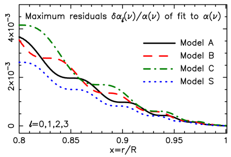
Fig. 14 shows the results - giving the maximum departure as a function of fractional radius on using the continuous phase shifts, the error decreases with increasing radius but is quite large at smaller radii. Clearly we should choose a fitting point for the phase matching well into the outer layers.
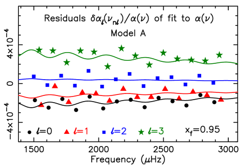
A further requirement is that the error in fitting the phase function for the discrete values with a series of Chebyshev polynomials (or any other set of basis functions), is sufficiently small not to be important in the phase matching algorithm. One way of testing this is to compare the from the continuous with those from using the discrete values. This is shown in Fig 15 for Model A at a fitting radius , where for the discrete values the average has been computed by fitting the full set of 56 with a series of Chebyshev polynomials up to degree 13. The errors are consistent with those from the continuous and lie in the range , demonstrating that the requirement on the errors is satisfied.
We then repeated the calculation for Models B, C and S and for mode sets of degree . The fractional errors are given in Table 5, along with the lowest values of in the full frequency set. All the errors are small but increase with decreasing frequency, and with increasing .
Table 5. Range of errors at - units
| values | Model S | Model A | Model B | Model C |
|---|---|---|---|---|
| 2218 | 1499 | 1121 | 566 | |
| 0,1 | -0.4 : 0.5 | -1.0 : 1.1 | -1.2 : 1.3 | -3.2 : 2.7 |
| 0,1,2 | -1.2 : 1.2 | -1.7 -: 2.1 | -2.0 : 2.1 | -4.1 : 4.1 |
| 0,1,2,3 | -1.8 : 2.8 | -2.7 : 3.6 | -3.1 : 4.3 | -5.8 : 5.8 |
We also checked the accuracy with which the continuous phase shifts, computed using the surface boundary condition that the oscillating potential and its derivative are zero at the surface, reproduce the exact values for the eigenfrequencies ; the fractional error is absolutely negligible: zero for and for for all 4 models. We also checked the error in using the Cowling approximation (neglect of the oscillating gravitational potential); here the error is of course zero for , but is still less than for for all 4 models.
The second criterion for the choice of the fitting point is that the s should not be influenced by the structure of the outer layers and in particular the HeII ionisation layer, since they then have a short period quasi periodic modulation of large amplitude, the choice of satisfies this criterion, as do other values in this region.
Although we calculate the continuous inner phase shifts by imposing the boundary condition on the gravitational potential at the surface, we also checked the error in imposing this condition at , the error is .
The error in taking limits the accuracy with which the phase function can collapse to a function only of frequency. For model A with and (see Fig 2), the dependent contribution to from the s is of order , whereas the dependence of is of order , much smaller than the contribution from the s.
For real data, with errors on the frequencies Hz, and a large separation Hz, the dominant error in comes from , larger than the errors from . We conclude that the approximation in the outer layers is valid.
The one exception is the Sun; with the very high precision achieved by space and ground based experiments it is necessary to take the outer phase shifts to be represented by two functions (cf Roxburgh & Vorontsov 1994b).
Acknowledgements
The author thanks Sergei Vorontsov for many valuable contributions to work on phase shift analysis over two decades, and Andrea Miglio for kindly providing his model set. He also gratefully acknowledges support from the Leverhulme Foundation under grant EM-2012-035/4.
References
- (1) Angulo, C and the NACRE consortium. 1999, Nuc. Phys. A, 656, 3-183
- (2) Appourchaux, T., Michel, E., Auvergne, M., et al. 2008, A&A, 488, 705
- (3) Benomar, O., Baudin, F., Campante, T. L., et al. 2009b, A&A, 507, L13
- (4) Benomar, O., Baudin, F., Marques, J. P., et al. 2010, AN, 331, 956
- (5) Bigot, L., Mourard, D., Berio, P., et al. 2011, A&A, 534, L3
- (6) Boyajian T S, van Belle G, & von Braun K, , 2013, ApJ, 771:40
- (7) Bruntt H, 2009, A&A, 506, 235
- (8) Christensen-Dalsgaard, J., Dappen, W., & Lebreton, Y. 1988, Nature, 336, 634-638
- (9) Christensen-Dalsgaard, J., et al., 1996. Science, 272, 1296-1292
- (10) Creevey, O. L., & Bazot, M. 2011, JPhCS, 271, 012038
- (11) Dziembowski, W. A., Paterno, L., & Ventura, R. 1988, A&A, 200, 213-217
- (12) Grevesse, N & Noels A, 1993. In Origin and Evolution of the Elements, ed.N Prantzos, E Vangioni-Flam, M Casse, pp. 15 25. Cambridge Univ. Press..
- (13) Ferguson J W, Alexander, D R, Allard D T, et al , 2005, ApJ, 623, 585 -596
- (14) Iglesias C A, Rogers, F J. 1996,, ApJ, 464, 943-953
- (15) Kallinger, T., Gruberbauer, M., Fossati, F.,& Weiss, W. W. 2010, A&A, 510, 106
- (16) Kjeldsen, H., Bedding T. R., Christensen-Dalsgaard, J., 2008. ApJ, 683: L175–178
- (17) Liu Z, Yang W, Bi S, et al, l 2014, ApJ, 780: 152
- (18) MacCullagh J, 1855, Trans Royal Irish Academy, vol XXII, part V, 387
- (19) Metcalfe, T. S., Creevey O. L., Christensen-Dalsgaard, J., 2009. ApJ, 699, 373-382
- (20) Miglio A, 2012 (private communication)
- (21) Piau, L., Turch-Chieze, S., Duez, V., et al. 2009, A&A, 506, 175
- (22) Rogers F J & Nayfonov A, 2002, ApJ 576, 1064-1074
- (23) Roxburgh, I.W. 1978,A&A, 65, 281
- (24) Roxburgh, I.W. 1989, A&A, 211, 361
- (25) Roxburgh, I.W. 2006, http://www.maths.qmul.ac.uk/~iwr/oscodes/L1modes.pdf
- (26) Roxburgh, I.W. 2008a Ap&SS, 316,141
- (27) Roxburgh, I.W. 2008b Ap&SS, 316, 75,
- (28) Roxburgh, I.W. 2009 A&A, 493,185,
- (29) RoxburghI W, 2010, Ap&SS, 328, 3
- (30) Roxburgh I W, 2014, ArkXiv, 1406, 1997
- (31) Roxburgh, I. W., & Vorontsov, S. V., 1994a MNRAS, 267, 297
- (32) Roxburgh, I. W., & Vorontsov, S. V., 1994b MNRAS, 268, 880
- (33) Roxburgh, I. W., & Vorontsov, S. V., 2000. MNRAS, 317, 141-150
- (34) Roxburgh, I. W., & Vorontsov, S. V., 2003. A&A, 411, 215-220
- (35) Roxburgh, I. W., & Vorontsov, S. V., 2006. MNRAS, 369, 1491
- (36) Roxburgh, I. W., & Vorontsov, S. V., 2013. A&A, 560, A2, 7pp
- (37) Scuflaire R et al, 2008, Ap&SS, 316, 83
- (38) Silva Aguirre, V., Basu, S., Brandao, I. M., et al. 2013, ApJ, 769, 141
- (39) Takata M, 2005, PASJ, 621, 750
- (40) van Leeuwen, F. 2007, A&A, 474, 653,