The Lyman-$\alpha$ forest in optically-thin hydrodynamical simulations

Abstract

We study the statistics of the Ly$\alpha$ forest in a flat $\Lambda$CDM cosmology with the $N$-body + Eulerian hydrodynamics code Nyx. We produce a suite of simulations, covering the observationally relevant redshift range $2\leq z\leq 4$. We find that a grid resolution of 20 $h^{-1}$kpc is required to produce one percent convergence of Ly$\alpha$ forest flux statistics, up to $k=10$ $h^{-1}$Mpc. In addition to establishing resolution requirements, we study the effects of missing modes in these simulations, and find that box sizes of $L>40$ $h^{-1}$Mpc are needed to suppress numerical errors to a sub-percent level. Our optically-thin simulations with the ionizing background prescription of Haardt & Madau (2012) reproduce an IGM density-temperature relation with $T_{0}\approx 10^{4}$ K and $\gamma\approx 1.55$ at $z=2$, with a mean transmitted flux close to the observed values. When using the ionizing background prescription of Faucher-Giguère et al. (2009), the mean flux is 10-15 per cent below observed values at $z=2$, and a factor of 2 too small at $z=4$. We show the effects of the common practice of rescaling optical depths to the observed mean flux and how it affects convergence rates. We also investigate the practice of ‘splicing’ results from a number of different simulations to estimate the 1D flux power spectrum and show it is accurate at the 10 per cent level. Finally, we find that collisional heating of the gas from dark matter particles is negligible in modern cosmological simulations.

1 Introduction

The cold dark matter (CDM) model of structure formation has proven impressively successful at describing observations on large scales and at early times. Perhaps the most successful confrontation of theory and observation is with the study of anisotropies in the cosmic microwave background, where such a comparison has yielded tight constraints on many of the basic cosmological parameters and an increased confidence in our understanding of the Universe in the linear regime. The next simplest structure is the intergalactic medium (IGM), the beaded filamentary network of structures between galaxies, which contains most of the mass in the Universe (for a recent review, see Meiksin, 2009). The IGM is best probed by the Ly$\alpha$ forest, the collection of intervening absorption systems detected in the spectra of distant quasars.

Ikeuchi (1986) and Rees (1986) were the first to suggest the Ly$\alpha$ forest originated from partially ionized hydrogen, in their case confined gravitationally by haloes of collisionless or cold dark matter. Using numerical simulations, Cen et al. (1994) demonstrated that Ly$\alpha$ forest systems arise naturally within the framework of theories of structure formation through gravitational instability in CDM dominated cosmologies. The installation of HIRES at Keck (Vogt et al., 1994) made it possible to make precision comparisons with the models, confirming the success of the gravitational instability scenario for the origin of the Ly$\alpha$ forest.

Modern hydrodynamic simulations recover many of the measured statistical properties of the Ly$\alpha$ forest, such as the H i column density distribution, the pixel flux distribution function and the flux power spectrum at a level capable of distinguishing between plausible variants of the CDM model, with the $\Lambda$CDM model the most successful (Zhang, Anninos & Norman, 1995; Hernquist et al., 1996; Rauch et al., 1997; Zhang et al., 1997; Croft et al., 1998; McDonald et al., 2000; Meiksin, Bryan & Machacek, 2001; Croft et al., 2002; Viel, Haehnelt & Springel, 2004). However, some differences are found. Most notable is the distribution of the absorption line widths (Doppler widths) characterized by the $b$-parameter (typically about 30 km/s). While the line widths are consistent with the amount of broadening characteristic of photoionized gas, the measured distributions show too many broadened lines compared with the predictions of the original simulations. This is likely an indication that He ii was reionized late, at $z\lesssim 4$ (Bryan & Machacek, 2000; Ricotti, Gnedin & Shull, 2000; Schaye et al., 2000; Meiksin, Bryan & Machacek, 2001; Worseck et al., 2014). Allowing for a late He ii reionization and including radiative transfer during reionization a range of Doppler widths may be achieved consistent with the data (Tittley & Meiksin, 2007; Meiksin & Tittley, 2012). Since the line widths control the scale and number of features, the distribution of wavelet coefficients is also strongly affected and, to a lesser extent, the column density distribution and the pixel flux distribution (Meiksin, Bryan & Machacek, 2001). The flux power spectrum is most affected at high wavenumbers.

The last decade has seen increasing use of Ly$\alpha$ absorption to investigate large- scale structure and cosmology. The Sloan Digital Sky Survey (SDSS) (York et al., 2000) provided an enormous increase in the amount of Ly$\alpha$ forest data with thousands of quasars suitable for 1D analysis, but at the cost of the spectra being low-resolution and fairly noisy. Still, this volume of data allowed a much-improved measurement of the 1D flux power spectrum (McDonald et al., 2006), placing constraints on the large scale spectral index $n_{s}$ and the amplitude of fluctuations $\sigma_{8}$. The BOSS experiment of SDSS-III (Dawson et al., 2013) further increased the sky density of suitable quasar lines of sight. The close proximity of large numbers of lines of sight has enabled 3D correlations in the forest to be measured over large scales for the first time using a sample of some 14000 QSOs (Slosar et al., 2011, 2013; Busca et al., 2013). The 3D flux information has also been cross-correlated with other high redshift tracers (Font-Ribera et al., 2012, 2013). The 1D flux power spectrum has been measured to unprecedented precision (Palanque-Delabrouille et al., 2013). The 3D Ly$\alpha$ absorption correlations are a promising means of constraining the nature of dark energy through the measurements of the angular diameter distance and the Hubble constant at high redshifts by detecting the large-scale Baryon Acoustic Oscillation (BAO) peak (Slosar et al., 2011; Busca et al., 2013; Font-Ribera et al., 2014). At the same time, the measured signal provides a novel test of the gravitational instability origin of the Ly$\alpha$ forest and the large-scale power in the meta-galactic ionizing background (e.g. McQuinn & White, 2011; McQuinn et al., 2011). In the near future, tomographic reconstruction with closely-separated Ly$\alpha$ forest sightlines from star-forming galaxies will enable direct 3D mapping of the IGM on $\sim$Mpc scales (Lee et al., 2014a).

The Ly$\alpha$ forest may also be used to constrain galaxy formation models. Galactic winds driven by feedback effects from galaxy formation models can impact statistics of the Ly$\alpha$ forest flux (Viel, Schaye & Booth, 2013) and the circumgalactic medium. Searches for the impact on the circumgalactic medium are underway around Lyman-break galaxies (Crighton et al., 2011; Rudie et al., 2012). Ly$\alpha$ forest simulations are required in this context to provide a quantitative interpretation of the results.

To fully compare numerical simulations with the growing body of increasingly accurate measurements of the Ly$\alpha$ forest, it is critical that the simulations have converged to a level of precision comparable to that of the data. Various studies have addressed convergence issues. These have tended to be heterogeneous, with conclusions dependent on the statistic for which convergence is sought, redshift, and cosmological model. We summarize the principal findings in the literature.

It is clear that the Jeans length of the gas ($\sim 500\,h^{-1}$kpc depending on the redshift) must be resolved to recover the correct absorption line widths and small-scale wavelet coefficients, with a suggested resolution of at least 40 $h^{-1}$kpc (comoving) at $z=2-3$ (Bryan et al., 1999; Schaye et al., 2000; Meiksin & White, 2001; Tytler et al., 2009; Lidz et al., 2010). Resolution on this scale is also adequate for converging to better than 5 percent on the hydrogen ionization rate required to match the measured effective optical depth of the IGM (Meiksin & White, 2004; Bolton et al., 2005; Tytler et al., 2009), as well as the effective optical depth itself (Bolton & Becker, 2009). At $z>4$, however, convergence on the effective optical depth diminishes to poorer than 15 percent at this mean resolution (Bolton & Becker, 2009). A resolution of 40 $h^{-1}$kpc is also inadequate for converging on the Doppler parameter and wavelet coefficient distributions at $z=4$. This is particularly the case for the narrowest features, for which a comoving mean resolution of better than 20 $h^{-1}$kpc appears necessary, with results still not clearly well converged (Bryan et al., 1999; Lidz et al., 2010).

The results are also sensitive to box size. The inferred mean ionizing background is converged to a few percent for comoving box sizes of 30 $h^{-1}$Mpc for $z>2$ (Meiksin & White, 2004; Bolton et al., 2005; Tytler et al., 2009). The linewidths increase with box size, possibly not converged to better than 5 percent at $z=2$ for a comoving box size as large as 54 $h^{-1}$Mpc (Tytler et al., 2009), although the distribution of smoothed wavelet coefficients appears well converged at this redshift for the smaller box size of 25 $h^{-1}$Mpc (Lidz et al., 2010). At $z>3$, the wavelet coefficients are not well converged for box sizes as large as 50 $h^{-1}$Mpc (Lidz et al., 2010).

Convergence requirements on the 1D flux power spectrum are also demanding. McDonald et al. (2005) found better than 5 percent convergence from the fundamental mode up to $k<0.025$ km^-1s for $2<z<4$, and up to $k<0.1$ km^-1s at $z<3$, for a resolution of 39 $h^{-1}$kpc, but in a comoving box size of only 5 $h^{-1}$Mpc. In larger boxes (30 $h^{-1}$Mpc), Viel & Haehnelt (2006) found 5 percent convergence at $k<0.01$ km^-1s for a mean resolution of 150 $h^{-1}$kpc, but of only 12 per cent for $k=0.02$ km^-1s at $z=4$. Other work found convergence of up to 10 per cent may be achieved at $k<0.03$ km^-1s in 20 - 40 $h^{-1}$Mpc boxes at $z=2-5$ (although possibly as poor as 20 per cent at $z=5$), with resolutions of 60 - 200 $h^{-1}$kpc, although requiring better than 50 $h^{-1}$kpc resolution for 5 percent convergence at $k=0.1$ km^-1s at $z=2$, with even this inadequate at $z=5$ (Meiksin & White, 2004; Bolton & Becker, 2009; Tytler et al., 2009). Even at this level, the spatial flux correlation function converges to better than 10 per cent over only 3 percent of the box size (Meiksin & White, 2004). The convergence of absorber pair and higher multiple statistics along neighboring lines of sight are not expected to fare better, which is perhaps why they have been largely ignored in simulation comparisons with data.

The primary goal of this paper is to establish the box size and resolution requirements to produce converged statistics of the Ly$\alpha$ forest flux over the redshifts of observational interest, with the minimum set of physical processes. While this is not the final word, doing so already presents several numerical challenges. The gaseous nature of the IGM requires simulating hydrodynamics along with the gravitating dark matter particles to obtain accurate results. Since the signals derive from almost the entire volume, and from the gas close to the mean density, Lagrangian methods which naturally increase resolution in the high-density regions are not favored in terms of ”time-to-solution”. In fact, they tend to be prohibitively expensive unless the hydrodynamic calculations are somehow truncated in the high density regions (e.g. by invoking artificial star formation as done in Gadget with the ‘Quick Lyman-alpha’ flag). Lagrangian methods will also have slightly worse resolution in underdense regions, which become important for the $z>3$ forest. In our code Nyx, we use an Eulerian (comoving) grid. Capturing the Jeans scale while covering a cosmologically representative volume requires a large dynamic range. Even with the modern supercomputers and a scalable cosmological hydrodynamics code, we are not able to directly simulate the volumes probed by observations while simultaneously resolving the Ly$\alpha$ forest. However, we are now able to simulate boxes large enough to be cosmologically representative and not suffer — to a desired accuracy — from the missing larger-scale modes.

The outline of the paper is as follows. In Section 2 we describe the physics and numerical capabilities required to simulate the IGM. Here we introduce our simulation code and the runs we performed for this study. We also describe how we model the Ly$\alpha$ forest using the simulation data. In Section 3 we discuss the physical properties of the IGM we find, and compare with previous results. In Section 4 we demonstrate the convergence of flux statistics with respect to physical resolution. We also explore the possibility of increasing the resolution via Richardson extrapolation. We demonstrate the convergence of flux statistics with respect to the domain size in Section 5. For the first time, we have produced simulations sufficiently large to capture large-scale effects while also resolving the Jeans scale. In Section 6 we compare our full-range simulation to a common technique for splicing together simulations with smaller dynamic ranges. It is commonly the case that simulations do not recover the observed mean flux, but that simulated fluxes are rescaled to match the observed mean. In Section 7 we explore effects of such rescaling. Statistics of Ly$\alpha$ lines and wavelets are presented in Section 8. In Section 9 we quantify the effects of collisionality between dark matter particles and gas which can artificially increase the temperature of the gas. Finally, we present our conclusions in Section 10.

Throughout this work, we assume the flat $\Lambda$CDM cosmological model. All distances are comoving and are quoted in “h units”, i.e. $h^{-1}$Mpc or $h^{-1}$kpc. Masses are in $\mathrm{M_{\odot}}$. When discussing the gas velocity, we use the peculiar velocity, $v=a\dot{x}$, where $x$ is the comoving scale. When discussing the velocity coordinate of a pixel, we use the Hubble flow velocity $v=\dot{a}x$, evaluated at that redshift.

2 Simulating the Ly-$\alpha$ Forest

Figure 1: A sample skewer, from a $2048^{3}$ simulation in a periodic box of side length $40\,h^{-1}$Mpc at $z=2.5$, showing the ingredients in the flux calculation. The top horizontal axis gives the (comoving) distance in the line-of-sight direction through the box. The lower horizontal axis gives the same distance in velocity units (see Table 1 for conversion factors). The top panel shows the baryon density, on a log scale. The middle panel illustrates how the velocity component along the line of sight $v_{\parallel}$ shifts the line center going from real- to redshift-space. The lower two panels show the optical depth and flux, respectively. The differences between the real- and redshift-space flux show that the redshift-space distortions do not just shift lines, but also change the blending of the lines.

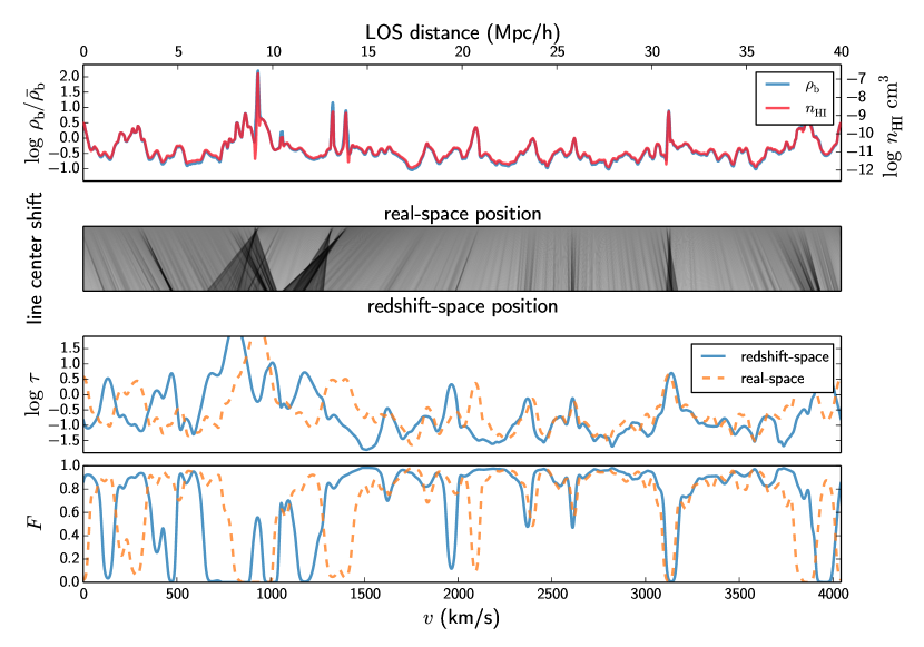
The Ly$\alpha$ forest arises primarily from four physical effects: the gravitational collapse of baryons and cold dark matter, ideal gas pressure support, radiative heating and cooling, and photoionization. The standard picture (see, e.g. Meiksin, 2009) is that at moderate overdensities and scales larger than $1\,h^{-1}$Mpc, the baryons simply trace the dark matter. The IGM at redshifts $z<6$ has a typical temperature $T\sim 10^{4}$ K, so that at scales of $\sim 100$ $h^{-1}$kpc the gas is pressure supported, and the density fluctuations are thus suppressed relative to the dark matter, or as often put, the baryons in the IGM are filtered on this scale. Gnedin & Hui (1998) first provided a detailed description of this process in the context of linear theory. Briefly, the scale at which the gravitational and pressure forces are equal is the Jeans length, and in comoving units is equal to

$$\lambda_{\rm J}=(1+z)c_{s}\sqrt{\frac{\pi}{G\rho_{\rm m}}}=0.783\sqrt{\frac{T/(10^{4}\,\mathrm{K})}{\Omega_{\rm m}(1+\delta)(1+z)}}\;h^{-1}\mathrm{Mpc}$$ (1)

In the case of adiabatic expansion (before reionization), $T\propto(1+z)^{2}$, the Jeans length decreases with time. In the case of constant temperature (after reionization) it increases with time. For the cosmology we assume here, with $\Omega_{\rm m}=0.275$, the Jeans length for mean density gas at $T=10^{4}$ K changes from 0.67 to 0.86 $h^{-1}$Mpc from $z=4$ to $z=2$. Observations suggest that the temperature of the IGM does not change much over the redshift range $2<z<4$ (Becker et al., 2011; Bolton et al., 2014), so we can immediately see that higher redshifts will require higher resolution to resolve Ly$\alpha$ forest absorbers to a similar accuracy.

As defined, the Jeans scale $k_{\rm J}=2\pi/\lambda_{\rm J}$ is an instantaneous measure that does not take into account the evolution of density or sound speed. Since the amount of filtering at a given epoch also depends on the thermal history of the gas, a more interesting dynamical quantity is the filtering scale $k_{\rm f}$, the scale at which baryon fluctuations are suppressed relative to cold dark matter. In linear theory, the filtering scale is

$$\frac{1}{k_{\rm f}^{2}(t)}=\frac{1}{D_{+}(t)}\int_{0}^{t}dt^{\prime}a^{2}(t^{\prime})\frac{\ddot{D}_{+}(t^{\prime})+2H(t^{\prime})\dot{D}_{+}(t^{\prime})}{k_{\rm J}^{2}(t^{\prime})}\int_{t^{\prime}}^{t}\frac{dt^{\prime\prime}}{a^{2}(t^{\prime\prime})}$$ (2)

The filtering scale in linear theory is always equal to the Jeans scale at an earlier time. This means that before reionization the filtering scale is larger than the Jeans scale, and after reionization the filtering scale is smaller than the Jeans scale. The key point here is that after reionization, in the case of roughly constant temperature history, $k_{\rm f}$ is smaller than the Jeans scale. A rule of thumb is that for typical growth factors and thermal histories, the filtering scale is roughly half the Jeans scale for $2<z<4$. In the linear regime the filtering of baryon power is roughly exponential:

$$P_{b}(k)\approx P_{\rm dm}(k)e^{-2k^{2}/k_{\rm f}^{2}}\;.$$ (3)

The chemical composition of the IGM is close to primordial, thus the dominant radiative processes involve only hydrogen and helium. The competition between photoionization heating and adiabatic cooling drives the gas to a tight power-law relation between density and temperature (Katz, Weinberg & Hernquist, 1996; Hui & Gnedin, 1997). As explained in Hui & Gnedin (1997), the slope of the power-law steepens in time, rapidly close to the reionization epoch, and more slowly in later times. After reionization, around $z=10$, the IGM is in photoionization equilibrium, with the ionization maintained by a UV metagalactic radiation field. The H i optical depth to Ly$\alpha$ scattering is proportional to the H i density, approximately described by a simple relation between the optical depth and baryon density:

$$\tau=A\left(\rho_{\rm b}/\bar{\rho}_{\rm b}\right)^{\beta}$$ (4)

Finally, the transmitted flux fraction is defined as $F=e^{-\tau}$, which we refer to as just flux. The normalization constant $A$ may be fixed by comparing with measurements of the mean Ly$\alpha$ transmission through the IGM, $\langle F\rangle\equiv\langle e^{-\tau}\rangle$.

Improvements on this method may be achieved by using a polytropic equation of state and approximating the density fluctuation distribution as lognormal (Bi & Davidsen, 1997) or using $N$-body simulations under the assumption that the baryons trace the dark matter, possibly with some pressure support (Petitjean, Mueket & Kates, 1995; Croft et al., 1998; Gnedin & Hui, 1998; Meiksin & White, 2001). While such simplified descriptions are sufficient for qualitatively characterizing the properties of the Ly$\alpha$ forest, they are unfortunately not adequate for detailed statistical predictions. In reality, we expect scatter in the $\rho_{\rm b}$-$T$ relation as a result of shock heating (as the peculiar velocities of most of the baryons are supersonic), other radiative processes, and possibly even He ii reionization at $2<z<4$. In addition, the relation between the local H i density and the flux is complicated by peculiar velocities along the line of sight.

As a result, it is likely that the most accurate description requires full hydrodynamical simulations coupled to an $N$-body code. Hydrodynamic simulations directly model the heating and cooling processes in the IGM, along with capturing the effects of shock heating. Pseudo-hydrodynamics methods like Hydro Particle Mesh (HPM) can capture the coarse properties of pressure support, but only shock-capturing methods can produce the correct $\rho_{\rm b}$-$T$ phases. As shown in Viel, Schaye & Booth (2013), capturing the hot gas that makes up the WHIM creates 5 per cent differences in the flux probability distribution function (PDF) and flux 1D power. In addition, accretion shocks on the outskirts of halos and filaments can clearly alter the density and temperature profiles of those regions and therefore the Ly$\alpha$ transmission through them.

The biggest computational challenge for accurately capturing the state of the IGM is the required dynamic range. In order to appropriately model bulk flows, simulations must cover linear scales of $\mathcal{O}(100\;h^{-1}\mathrm{Mpc})$. The bulk flows play an important role in determining the temperature distribution of the IGM via shock heating. As shown in Tytler et al. (2009), using too small a box will result in an underestimate of the mean temperature $T_{0}$. At the same time, simulations must resolve the filtering scale, which is $\mathcal{O}(100\;h^{-1}\mathrm{kpc})$ for the densities of interest. The required dynamic range ends up being closer to $10^{4}$ than $10^{3}$ however, because adequately resolving a given scale in a simulation means covering it with several resolution elements, so the required minimum scale turns out to be 10 to 20 $h^{-1}$kpc.

With modern numerical techniques and supercomputers, resolving a dynamic range of $\sim 10^{4}$ in full volume of a 3D simulation is now practical. Using Lagrangian techniques like Smoothed Particle Hydrodynamics (SPH) or the Eulerian adaptive resolution technique Adaptive Mesh Refinement (AMR), it is straightforward to achieve still larger dynamic ranges. However, these techniques only help simulations focused on resolving small fractions of the total domain volume. The difficulty in simulating the IGM is that it covers almost all of the volume of the domain. The gas responsible for the Ly$\alpha$ forest is close to the cosmic mean density rendering Lagrangian methods computationally non-optimal as they spend a majority of the compute cycles evolving dense regions. This is especially true at higher redshifts where most of the signal comes from the underdense regions (Fig. 7).

The Ly$\alpha$ forest arises from relatively low column density regions, with the contribution from higher column densities decreasing as a power law. Lines with low hydrogen column density are difficult to observe in practice, thus observations recover well lines with $N_{\textrm{H}\,\textsc{i}}>10^{13}$ cm^-2, especially at high redshifts, $z>2$ (see, e.g.  Janknecht et al., 2006; Haardt & Madau, 2012). In these environments the H i ionizing photon mean free path is much larger than the boxes simulated here for $z<6$. Therefore we model radiative processes under the assumption of an optically-thin medium and assume a uniform ionizing background radiation field. We note that accurate modeling of high column density systems, like Lyman limit systems with $N_{\textrm{H}\,\textsc{i}}>10^{17}$ cm^-2, or Damped Ly$\alpha$ systems characterized by $N_{\textrm{H}\,\textsc{i}}>10^{20}$ cm^-2, should include explicit radiative transfer. While these systems do form in our simulations, the relevant physics is not present in our optically thin simulations and we shall not investigate them in detail.

Table 1: Conversion factors versus redshift

$z$	$\lambda_{\alpha}$	$H(z)$	$d\lambda/d\chi$	$dv/d\chi$	$10^{3}dz/d\chi$
2.00	3645	285	1.16	95	0.95
2.25	3949	319	1.29	98	1.06
2.50	4253	354	1.43	101	1.18
3.00	4860	428	1.73	107	1.42
3.50	5468	508	2.06	113	1.69
4.00	6075	592	2.40	118	1.98

Conversion factors for the flat $\Lambda$CDM cosmology considered here with $h=0.702$ and $\Omega_{\rm m}=0.275$. Wavelengths are given in Å, comoving distances in $h^{-1}$Mpc and velocities in km s^-1.

Hydrogen (and HeI) reionization takes place at high redshift, $z>10$. Therefore the details of this epoch are unimportant for the thermodynamical properties of the gas at redshifts relevant for Ly$\alpha$ forest observations ($z<4$). In contrast, He ii reionization takes place at an observationally relevant epoch ($3<z<5$) although the observational picture is not yet resolved (e.g. Worseck et al., 2014). In addition, the size of fluctuations in the He ii ionizing background are very poorly constrained, varying by an order of magnitude in recent studies (Shull et al., 2010; Syphers & Shull, 2014; McQuinn & Worseck, 2014). However, the main effect of He ii reionization on the IGM is that the additional photoheating increases the temperature of the IGM. The UV background prescriptions we employ in this study model this increase in the temperature via an increase in photoheating rates and ionize He ii by $z=3$. We note, however, that He ii reionization could result in higher temperatures with explicit radiative transfer and significant (spatial) fluctuations of the ionizing background. Thus, including He ii reionization correctly in simulations requires incorporating radiative transfer (Tittley & Meiksin, 2007), which remains an active area of current research in cosmological hydrodynamics codes (Tittley & Meiksin, 2007; McQuinn et al., 2011; Meiksin & Tittley, 2012; Compostella, Cantalupo & Porciani, 2013).

2.1 Simulations

The simulations we present here are performed with the Nyx code (Almgren et al., 2013). Nyx follows the evolution of dark matter simulated as self-gravitating Lagrangian particles, and baryons modeled as an ideal gas on a uniform Cartesian grid. Nyx includes Adaptive Mesh Refinement (AMR) capabilities, which we can use to extend the simulated dynamic range. We do not make use of AMR in the current work, as the Ly$\alpha$ forest signal spans nearly the entire simulation domain rather than isolated concentrations of matter where AMR is more effective. The Eulerian gas dynamics equations are solved using a second-order accurate piecewise parabolic method (PPM) to accurately capture shock waves. Our implementation uses a dimensionally unsplit scheme with full corner coupling (Colella, 1990) to better reconstruct the 3D fluid flow. The same mesh structure that is used to update fluid quantities is also used to compute the gravitational field and to evolve the particles via a particle-mesh (PM) method, using Cloud-In-Cell (CIC) interpolation to switch between particle- and mesh-based quantities. The gravitational source terms in the momentum and energy equations are discretized in time using a predictor-corrector approach. The additional physics of radiative heating and cooling is included via source terms in the equations for internal and total energy. As the relevant time scale for heating and cooling can be significantly different from the stability criterion required by the explicit discretization of gas dynamics equations (the Courant-Friedrichs-Lewy or CFL condition), the heating and cooling source terms are integrated in time using VODE (Brown, Byrne & Hindmarsh, 1989) and coupled to the hydrodynamics using a Strang splitting (Strang, 1968) approach. For more details of our numerical methods, see Almgren et al. (2013).

Table 2: List of simulations

Name	Box size	Elements	Resolution	$m_{\rm dm}$
	[$h^{-1}$Mpc]		[$h^{-1}$kpc]	[$\mathrm{M_{\odot}}$]
L10_N128	10	1283	78	$4.3\times 10^{7}$
L10_N256	10	2563	39	$5.4\times 10^{6}$
L10_N512	10	5123	20	$6.7\times 10^{5}$
L10_N1024	10	10243	10	$8.4\times 10^{4}$
L20_N256	20	2563	78	$4.3\times 10^{7}$
L20_N512	20	5123	39	$5.4\times 10^{6}$
L20_N1024	20	10243	20	$6.7\times 10^{5}$
L20_N2048	20	20483	10	$8.4\times 10^{4}$
L40_N512	40	5123	78	$4.3\times 10^{7}$
L40_N1024	40	10243	39	$5.4\times 10^{6}$
L40_N2048	40	20483	20	$6.7\times 10^{5}$
L80_N1024	80	10243	78	$4.3\times 10^{7}$
L80_N2048	80	20483	39	$5.4\times 10^{6}$
L80_N4096	80	40963	20	$6.7\times 10^{5}$

The simulations used in this work. Resolution refers to the cell size, and to ease comparison with SPH simulations we list the mass of dark matter particles in each simulation. See text for details.

We simulate the WMAP 7-yr data constrained $\Lambda$CDM cosmology, with parameters: $\Omega_{\rm m}=0.275$, $\Omega_{\Lambda}=1-\Omega_{\rm m}=0.725$, $\Omega_{\rm b}=0.046$, $h=0.702$, $\sigma_{8}=0.816$, and $n_{s}=0.96$ (Komatsu et al., 2011). We provide Table 1 to help convert between scale, wavelength, and velocity coordinates at redshifts used in this work. The latest Planck constraints (Planck Collaboration et al., 2014) differ somewhat from WMAP-7 values, most notably in the values for the Hubble constant $h$ and total matter content $\Omega_{\rm m}$. These differences will not play an important role in this paper, as we aim to explore numerical prescriptions for achieving 1 per cent accurate Ly$\alpha$ forest statistics. The conclusions here will inform future work for running many viable cosmologies and understanding their numerical limitations.

The full set of simulations is listed in Table 2. We designed the set of simulations to cover the expected maximum box size and minimum resolution needed to show convergence. All simulations are initialized at $z=159$, starting from a grid distribution of particles and Zel’dovich approximation (Zel’dovich, 1970). Transfer functions were generated using both analytical approximation Eisenstein & Hu (1999) and Boltzmann solver code CLASS (Blas, Lesgourgues & Tram, 2011). The conclusions presented here have no sensitivity on the particular transfer function used, but it is of course important to maintain the same transfer function accross a series of runs one is comparing to each other. We focus on snapshots in the range $2\leq z\leq 4$, relevant for most observations. To simplify the comparison, simulations performed in the same box size share the same large-scale modes, the only difference being that higher resolution runs have more modes sampled on small scales.

Figure 2: A slice of the baryon density, temperature, H i number density, and flux from the L20_N2048 simulation at $z=2.5$. The slice covers the domain of 20 x 20 $h^{-1}$Mpc, with a thickness of about 100 $h^{-1}$kpc (10 cells). Note that the $F$ line of sight is the y-axis direction, so that broadened lines show up as vertical black streaks.

2.2 Included Physics

Besides solving for gravity and the Euler equations, we model the chemistry of the gas as having a primordial composition with hydrogen and helium mass abundances of $X=0.75$, and $Y=0.25$, respectively. The choice of values is in agreement with the recent CMB observations and Big Bang nucleosynthesis (Coc, Uzan & Vangioni, 2013). The resulting reaction network includes 6 atomic species: H i, H ii, He i, He ii, He iii and e^-, which we evolve under the assumption of ionization equilibrium. The resulting system of algebraic equations is:

$$\left(\Gamma_{e,\textrm{H}\,\textsc{i}}n_{e}+\Gamma_{\gamma,\textrm{H}\,\textsc{i}}\right)n_{\textrm{H}\,\textsc{i}}=\alpha_{\rm r,\textrm{H}\,\textsc{ii}}n_{e}n_{\textrm{H}\,\textsc{ii}}$$ (5)

$$\left(\Gamma_{e,\textrm{He}\,\textsc{i}}n_{e}+\Gamma_{\gamma,\textrm{He}\,\textsc{i}}\right)n_{\textrm{He}\,\textsc{i}}=\left(\alpha_{\rm r,\textrm{He}\,\textsc{ii}}+\alpha_{\rm d,\textrm{He}\,\textsc{ii}}\right)n_{e}n_{\textrm{He}\,\textsc{ii}}$$

$$\left[\Gamma_{\gamma,\textrm{He}\,\textsc{ii}}+\left(\Gamma_{e,\textrm{He}\,\textsc{ii}}+\alpha_{\rm r,\textrm{He}\,\textsc{ii}}+\alpha_{\rm d,\textrm{He}\,\textsc{ii}}\right)n_{e}\right]n_{\textrm{He}\,\textsc{ii}}$$

$$\qquad=\alpha_{\rm r,\textrm{He}\,\textsc{iii}}n_{e}n_{\textrm{He}\,\textsc{iii}}+\left(\Gamma_{e,\textrm{He}\,\textsc{i}}n_{e}+\Gamma_{\gamma,\textrm{He}\,\textsc{i}}\right)n_{\textrm{He}\,\textsc{i}}$$

in addition, there are three closure equations for the conservation of charge and hydrogen and helium abundances. Radiative recombination ($\alpha_{\rm r,X}$), dielectronic recombination ($\alpha_{\rm d,X}$), and collisional ionization ($\Gamma_{e,{\rm X}}$) rates are strongly dependent on the temperature, which itself depends on the ionization state through the mean mass per particle $\mu$

$$T=\frac{2}{3}\frac{m_{p}}{k_{\rm B}}\mu\ e_{\rm int}$$ (6)

where $m_{p}$ is the mass of a proton, $k_{\rm B}$ is the Boltzmann constant, and $e_{\rm int}$ is the internal thermal energy per mass of the gas. Here we assume adiabatic index for monoatomic ideal gas. For a gas composed of only hydrogen and helium, $\mu$ is related to the number density of free electrons relative to hydrogen by $\mu=1/\left[1-(3/4)Y+(1-Y)n_{e}/n_{\rm H}\right]$. We iteratively solve the reaction network equations together with the ideal gas equation of state, $p=2/3\rho e_{\rm int}$, to determine the temperature and equilibrium distribution of species.

We compute radiative cooling as in Katz, Weinberg & Hernquist (1996), and assume a spatially uniform, but time-varying ultraviolet background (UVB) radiation field from either Faucher-Giguère et al. (2009) or Haardt & Madau (2012). We do not follow radiation transport through the box, nor do we explicitly account for the effects of thermal feedback of stars, quasars, or active galactic nuclei; all cells are assumed to be optically thin, and radiative feedback is accounted for via the UVB model. In addition, we include inverse Compton cooling off the microwave background. For the exact rates used in the Nyx code and comparison of two UV backgrounds we refer the reader to Appendix A.

2.3 Simulated Spectra

The optical depth $\tau$ for Ly$\alpha$ photon scattering is

$$\tau_{\nu}=\int n_{\rm X}\sigma_{\nu}dr$$ (7)

where $\nu$ is the frequency, $n_{\rm X}$ is the number density of species X, $\sigma_{\nu}$ is the cross section of the interaction, and $dr$ is the proper path length element. For our current work, we assume a Doppler line profile, so the resulting optical depth is

$$\tau_{\nu}=\frac{\pi e^{2}}{m_{e}c}f_{12}\int\frac{n_{\rm X}}{\Delta\nu_{\rm D}}\frac{\exp\left[-\left(\frac{\nu-\nu_{0}}{\Delta\nu_{\rm D}}\right)^{2}\right]}{\sqrt{\pi}}dr,$$ (8)

where $\Delta\nu_{\rm D}=(b/c)\nu_{0}$ is the Doppler width with the Doppler parameter $b=b_{\rm thermal}=\sqrt{2k_{\rm B}T/m_{\rm H}}$, and $f_{12}$ is the upward oscillator strength of the Ly$\alpha$ resonance transition of frequency $\nu_{0}$. See Appendix B for a more detailed discussion of our optical depth calculation, including the discretization of Equation (8).

We choose sightlines, or “skewers”, crossing the domain parallel to one of the axes of the simulation grid and piercing the cell centers. Computationally, this is the most efficient approach. This choice of rays avoids explicit ray-casting and any interpolation of the cell-centered data, which introduce other numerical and periodicity issues. We cover the entire $N^{3}$ grid with skewers, which provides the equivalent of $N^{2}$ spectra. Although large-scale modes along different spatial dimensions are statistically independent allowing some gain in statistics from multiple viewing directions, in this work we use a single line-of-sight axis rather than combining together skewers using all 3 axes. The process of going from simulated baryon values to flux $F$ is illustrated in Figure 1.

3 Physical Properties of the Ly$\alpha$ Forest

Figure 3: The density–temperature distribution of gas (volume-weighted histogram) at $z=2.5$ in the L40_N2048 simulation, showing broadly four thermodynamical regimes for baryons in cosmological simulations. Simulation was done with Haardt & Madau (2012) UV background. The Ly$\alpha$ forest signal primarily comes from the diffuse region in the lower-left, which includes most of the baryons in the universe. Note the tight temperature-density relation in this regime.

Zhang et al. (1998) discuss the physical properties of the Ly$\alpha$ forest in hierarchical models such as CDM. The discussion in this section can largely be considered as an update of that work.

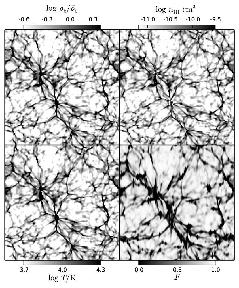
As described above, the state of the IGM is relatively simple with a few power laws approximately tying together the spatial distribution of baryon density, temperature, proper H i number density, and optical depth to H i Ly$\alpha$ photon scattering. Figure 2 shows a slice of these quantities in one of our high-resolution simulations, except with the optical depth replaced by the transmitted flux. We choose to show flux because it highlights the range of each quantity that is relevant for observations. That is, we want to highlight differences between an optical depth of 1 or 2, which changes the flux drastically, but not between 10 and 100, which is essentially opaque. We adjusted the gray-scale intensity ranges of density, temperature, and H i number density to roughly match the morphology of the flux, which provides a good guide to what ranges of each quantity affects the Ly$\alpha$ forest. We note that over the relevant redshift range, the comoving density and temperature evolve slowly, so that these ranges roughly apply to all redshifts. However, the physical H i density changes drastically primarily due to expansion. The striking morphological similarity between the fields demonstrates how well the usual approximations work. The flux field is clearly the least like the other fields due to two effects: the optical depth is in redshift-space and is therefore distorted by peculiar velocities; in addition it is also thermally broadened, smearing high temperature regions across the line-of-sight axis.

A key component of the robustness of Ly$\alpha$ forest predictions is the $\rho_{\rm b}$-$T$ relation in the diffuse IGM. The relation is approximated by the power law

$$T=T_{0}\left(\frac{\rho_{\rm b}}{\bar{\rho}_{\rm b}}\right)^{\gamma-1}$$ (9)

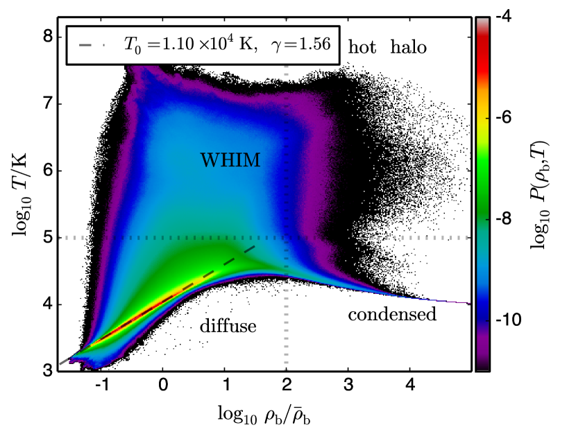
where $T_{0}$ is the temperature at mean density, and $\gamma$ is the slope of density-temperature relation, both of which are set by the metagalactic ionizing background. Typical values are $T_{0}$ between 10,000 and 20,000 K and $\gamma$ between 1 and $1.6$. Figure 3 shows the joint PDF of density and temperature (volume-weighted) in the L40_N2048 as an image and the power law relation over plotted with a dashed line. We tried fitting the density-temperature relation line several ways and found that a linear least-squares fit is sufficient. The number of points in the diffuse IGM phase is very large even for small simulations, so there is very little uncertainty in the fit parameters. However, we noticed a small but systematic difference in the best-fit $\gamma$ depending on the density range fit. Fitting underdense regions, i.e. points with $-1<\log_{10}\rho_{\rm b}<0$ yields $\gamma$ values a few percent higher than fitting near the mean density, $-0.5<\log_{10}\rho_{\rm b}<0.5$. Thus even if we neglect the scatter in the $\rho_{\rm b}$-$T$ relation a single power-law approximation breaks down at a few percent accuracy.

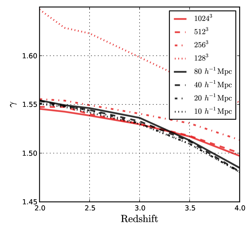
Figure 4 shows the evolution of our best-fit values for $\gamma$ in the resolution series of simulations and the box size series of simulations. We fit the $\rho_{\rm b}$-$T$ relation with linear least squares in $\log\rho_{\rm b}$ and $\log T$, fitting the range $-0.5<\log_{10}\rho_{\rm b}<0.5$ and $\log_{10}T/\mathrm{K}<4$. We see that convergence with spatial resolution is rather fast, and that box size does not affect recovered value of $\gamma$. In addition, we see that UV background as given by Haardt & Madau (2012), shown in black, exhibits marginally more redshift evolution than that of Faucher-Giguère et al. (2009) (the red lines in Figure 4). We find similar results in the fit $T_{0}$ values, where there is a small resolution effect for poor resolution, but the fit value remains the same between the L10_N256, 512, and 1024 runs. Box size appears to have no effect on the resulting $\rho_{\rm b}$-$T$ line, as expected.

Figure 4: Redshift evolution of $\gamma$, the slope of density-temperature relation. Lines in black show the weak dependence on the box size (the resolution is kept fixed at 20 $h^{-1}$kpc), while the the red lines show a rapid convergence with respect to the spatial resolution (in 10 $h^{-1}$Mpc box). Black and red lines are simulations with Haardt & Madau (2012) and Faucher-Giguère et al. (2009) UV backgrounds, respectively.

A large fraction of the gas lies on the $\rho_{\rm b}$-$T$ relation line — about 90 per cent by volume and 50 per cent by mass in this case. The significant scatter above the power-law relation line is due to shock heating, whereas the small scatter just below the line is due to a subtlety in the discretization of the gravitational source term in the total energy equation. As discussed in Almgren et al. (2013), the most obvious discretization is to compute the product of the momentum and the gravitational vector. While this is spatially and temporally second-order accurate, it allows gravitational work to change the internal energy since the update to the total energy is no longer numerically equivalent to the update to the kinetic energy calculated using the updates to the momenta. An alternative discretization defines the update to total energy only through the update to kinetic energy as calculated from the momentum equation. This maintains the analytically expected behavior of gravitational work contributing to the kinetic energy only. Through numerical testing we have determined that the latter formulation greatly reduces the number of cells scattered below the line in void regions, while having a negligible effect on the results otherwise. Due to the small number of cells affected, the difference to the flux mean, pdf, and power spectrum at $k\leq 10$ $h^{-1}$Mpc is only 0.1%. The fraction of gravitational work in a timestep that directly contributes to the internal energy (thereby increasing the temperature) rather than kinetic energy ranges from $5\times 10^{-3}$ at early times to $5\times 10^{-2}$ at late times for a run with CFL number of 0.5. These numbers are quite independent of the spatial resolution employed. However, while the two discretizations of the gravitational source produce this difference in $\rho_{\rm b}$-$T$ regardless of the spatial resolution, they do converge to the same answer when refining the time-step: in simulations run with a CFL number of 0.05, the two formulations yield indistinguishable $\rho_{\rm b}$-$T$ plots, and the fraction of gravitational work that contributes to the internal energy stays below $5\times 10^{-3}$ throughout the run.

Figure 5: The mean temperature of the IGM as a function of redshift in our simulations compared to the observations presented in Becker et al. (2011) (error bars are 2-$\sigma$). The red line shows a simulation using Katz, Weinberg & Hernquist (1996) atomic rates and the Faucher-Giguère et al. (2009) UVB. The blue line is obtained using the rates presented in the Appendix A of this paper and Faucher-Giguère et al. (2009) UVB. The black line shows a simulation with the rates presented in Appendix A and the Haardt & Madau (2012) UVB. While the main figure shows the $T_{0}$ evolution over the observationally relevant redshifts, the inset figure shows the full simulation range starting at $z=159$, on a logarithmic scale.

In Figure 3, we have also roughly marked the four phases of the IGM: the diffuse IGM giving rise to the Ly$\alpha$ forest, the Warm Hot IGM (WHIM) — rarefied, shocked gas falling onto the filaments and halos, the hot halo gas in the process of virialization, and the cooling and collapsing condensed phase. The overall shape of the $\rho_{\rm b}$-$T$ diagram is reproduced in almost any cosmological simulation, even with low-resolution, as long as it includes primordial gas heating and cooling. However, we do find that larger box size simulations produce more shocked gas around filaments (a more significant WHIM). We do not see a significant resolution dependence on the fraction of gas in the WHIM, but we see both that larger boxes have more gas in the WHIM, and that the WHIM is shocked to higher temperatures. This is expected behavior, as small-box simulations miss large-scale velocity components. For the most interesting, diffuse gas region, the $\rho_{\rm b}$-$T$ relation and the amount of scatter around it can also be affected by He ii reionization. For instance, McQuinn et al. (2009) found that in their post-processed radiative transfer simulations most of the reionization models increased $T_{0}$ and decreased $\gamma$ while significantly broadening the $\rho_{\rm b}$-$T$ relation, mostly due to spatial variations in the $\rho_{\rm b}$-$T$ relation from RT effects like shadows. Understanding the full effects of He ii reionization on IGM is beyond the scope of this work.

Figure 6: Illustration of the effect of the filtering scale on power spectra. Here we show the power spectra of baryon density $\rho_{\rm b}$, dark matter density $\rho_{\rm dm}$, the local flux $F_{\rm local}$, the monopole of the redshift-space (observable) flux $F$, and the thresholded baryon density $\rho_{\rm b,thr}$ limited to 100, 10, and 3 times the mean density, all from the L40_N2048 simulation at redshift $z=2$.

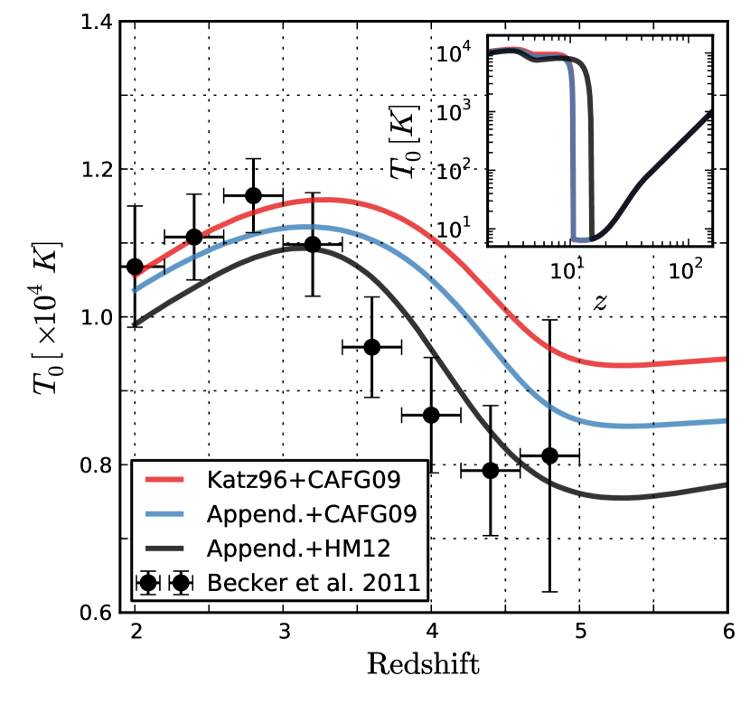
In Figure 5, we show the evolution of the temperature at mean density. This is calculated as an average (in log space) of the gas at mean density for temperatures $T<10^{5}$ K at each time step. We also show the effects of different UV backgrounds, from Faucher-Giguère et al. (2009) and Haardt & Madau (2012), and differing atomic rates (see Appendix A). Qualitatively the temperature of the IGM decreases at high redshifts due to the expansion and inverse Coulomb cooling, then rises sharply during hydrogen reionization at $z\sim 10$. We carried out a study spanning several orders of magnitude in initial temperature for our simulations and have determined that, due to adiabatic expansion, Compton cooling and hydrogen reionization, no memory of the initial temperature is retained at $z\lesssim 10$. In Figure 5, we also show recent observational results from Becker et al. (2011), which is in good agreement with the $z=2.4$ measurement recently carried out by Bolton et al. (2014) but lower than the temperatures inferred by Lidz et al. (2010). It is interesting to point out that the differences in temperature evolution that different modern UV backgrounds produce, roughly 10 per cent, are less than observational uncertainties. We also note that both of the UV backgrounds we consider show two visible jumps in the temperature of the IGM, corresponding to H i and He ii reionizations.

Figure 7: Contribution of different density regions to the Ly$\alpha$ forest flux at $z=2$, 3, 4. Meax flux was rescaled to match Becker et al. 2011. Left: the real-space flux vs. gas density. The lines show the medians and the filled regions show the normalized median absolute deviation (normalized to match one standard deviation for a normal distribution). Middle: the redshift-space flux vs. gas density. Right: the cumulative distribution of mass vs. redshift-space flux.

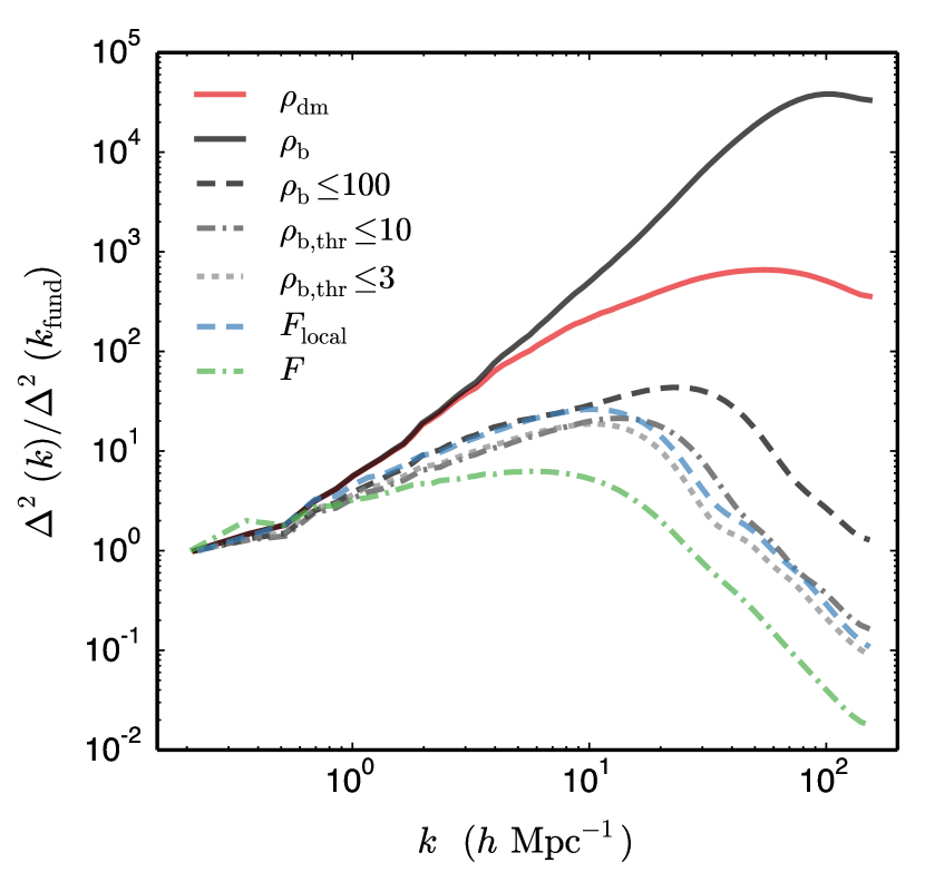
Due to the direct influence of pressure forces, baryon fluctuations are suppressed compared to dark matter (which is affected by the gas pressure only because the gravitational acceleration has a component due to the gas). Our simulations do not account for the details of star formation, feedback from stars or Active Galactic Nuclei; the regions that should be galaxies are only blobs of overcooled gas. Due to this overcooling inside halos, small-scale fluctuations in the baryonic component are artificially enhanced as shown in the solid black line of Figure 6 (the red line shows the dark matter power spectrum for reference). Since we know that our simulations do not realistically represent the gas quantities in high density regions, we can exclude them from our analysis at which point the filtering scale becomes clear. To highlight this, in Figure 6, we show the baryon power spectrum with several density thresholds. These are obtained by “clipping” the original baryon density field, i.e. resetting the densities higher than the threshold down to the selected threshold value. The clipping is done here only for illustrative purposes. This is qualitatively similar to what happens with the Ly$\alpha$ forest signal — where the flux drops to zero at a certain density, and any higher density has no additional effect. Clipping of the small-scale fluctuations also introduce a linear bias on large scales. For clarity, we have normalized all power spectra to be 1 at the fundamental (box-scale) mode. The different threshold value power spectra also illustrate that there is a density dependence of the filtering scale. As the threshold density decreases, the filtering scale increases. We also show two flux power spectra to see how they probe the filtering and thermal broadening scale. We computed the Ly$\alpha$ forest flux without redshift-space distortions or thermal broadening, which we call the local flux $F_{\rm local}$. In this case, the optical depth for the local flux is just the appropriate rescaling of the H i number density,

$$\tau_{\rm local}=\frac{\pi e^{2}f_{lu}\lambda_{0}}{m_{e}cH(z)}n_{\textrm{H}\,\textsc{i}}\;;\;F_{\rm local}=e^{-\tau_{\rm local}}\;.$$ (10)

The dashed blue line is the local flux spectrum, which shows pressure support smoothing at a scale roughly matching the $\rho_{\rm b,thr}\leq 10$ result. Note the little difference between thresholding at 10 times the mean baryon overdensity and 3 times the mean. We also show the monopole of the 3D flux power spectrum as the dashed green line, which includes smoothing not just from pressure support but also contributions from thermal broadening and redshift-space distortions, giving rise to even more filtering on small scales.

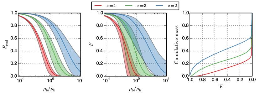
In Figure 7, we show relations between the Ly$\alpha$ forest flux and the gas density. In the left panel we plot the real-space flux of cells as a function of gas density. For each density bin we plot the median and normalized median absolute deviation (normalized to equal the standard deviation for a normal distribution) independently above and below. This serves as a qualitative estimate of what density regimes contribute to the Ly$\alpha$ forest signal at different redshifts. For instance, we immediately see that a majority of the signal at high redshift originates in under-dense regions, while at $z=2$, it lies in the mild overdensities. In the middle panel, we show similar info, but this time we use the redshift-space flux. As redshift-space distortions couple regions several Mpc away and can map different cells to the same redshift-space position (see Figure 1), the redshift-space flux is less correlated with density and thus exhibits more scatter than in real space. However, the median lines are similar at all redshifts. In the right panel, we show the cumulative mass of cells with fluxes above some value. The sharp rise in the cumulative mass at $F=0$ shows the mass fraction in the saturated regions of the forest, filaments and halos. This figure also shows the difficulty of simulating Ly$\alpha$ forest signal at high redshifts, $z\gtrsim 4$: we immediately see that small fluctuations in density produce significant difference in flux. Arguably, this effect is more critical for numerical convergence than the decrease in filtering scale described in Section 2.

Historically, the Ly$\alpha$ forest was studied in the context of absorption line systems. However, the process of Ly$\alpha$ forest line finding and fitting is not well-defined and results can vary between implementations. For this reason we will explore line statistics separately in Section 8, and in the following sections we will focus on the flux $N$-point correlation statistics.

4 Resolution study

Figure 8: Illustration of the effects of resolution in the 10 $h^{-1}$Mpc simulations at $z=2.5$. On the left, we plot slices $\sim 150$ $h^{-1}$kpc deep (2 cells in the 128³ simulation) of the baryon density. On the right we show values along the skewers marked as dashed lines in the slices. The skewers were selected in the same position in each simulation.

The physical resolution required to model Ly$\alpha$ forest flux statistics varies significantly with redshift, with higher redshifts requiring higher resolution for the same relative error. There are several physical effects which contribute to this behavior. One is the change in the comoving filtering scale, which decreases with increasing $z$. We further demonstrate the increasing steepness of the flux–density correlation as a function of redshift in Figure 7, which means that for the same relavite error in $\rho_{b}$ or $N_{\textrm{H}\,\textsc{i}}$ the relative error in flux will be larger at $z=4$ than at $z=2$. Finally, the gas in voids is $\sim$2 times colder than the gas at the mean density (and a factor of $\sim$4 colder than in mild overdensity regions), therefore thermal broadening of lines is less at high redshifts than at low ones.

The average transmission sharply increases going to lower redshifts as the physical density of neutral hydrogen decreases, primarily due to the expansion of the universe, with secondary changes due to the ionizing background radiation. Here we explore the accuracy of simulated Ly$\alpha$ forest flux statistics at $2\leq z\leq 4$, the relevant range for most of current and near future observations. We focus on results in our 10 $h^{-1}$Mpc boxes, as they offer the easiest path to an increase in resolution, but we have also explicitly checked that the conclusions presented here are valid in the case of the larger-box simulation series as well (see Table 2). In other words, we do not observe that numerical errors due to missing modes (explored in the next section of this paper) couple with resolution error at more than the percent level. The same behavior was observed in Gadget simulations presented in Stark et al. (2014). The simulations we present in this section were done with Faucher-Giguère et al. (2009) UV backround.

The results of this section are applicable to grid/Eulerian codes, where the effective resolution of pressure forces is commonly better than the effective resolution of gravitational forces. For example, many tests show that hydrodynamic quantities are already very accurate at 1 - 2 cells away from discontinuities — see e.g. Almgren et al. (2010) for the case of the hydro algorithm implemented in Nyx but the same is true for schemes used in virtually any other cosmological Eulerian hydro code to date. On the other hand, the gravitational force resolution is much worse. Grid codes use a Particle-Mesh (PM) scheme to compute gravitational forces, which is very fast but suffers from smoothing the density field at small scales. Generally, two particles must be separated by at least 5 cell sizes for the gravitational force to match $1/r^{2}$ (for example, see Habib et al. 2009). The opposite is true in most SPH Ly$\alpha$ forest simulations presented in the literature. In this case, gravitational resolution is much higher for the same grid size/number of particles, with the gravitational forces computed with a TreePM or particle-particle PM hybrid scheme. This provides a much (roughly 10 times) higher gravitational resolution than the grid codes for the same grid configuration. At the same time, the SPH kernel smooths the hydrodynamic quantities on scales of $\sim 2\times$ the mean inter-particle spacing for gas around mean density. In this regard, the resolution study presented here is not directly applicable to all codes. However, we believe that the results of other studies we conduct in this paper are largely code independent.

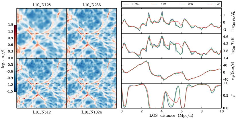
In Figure 8, we provide an illustration of how the grid resolution affects relevant IGM structures and the Ly$\alpha$ forest flux. Here we use our four 10 $h^{-1}$Mpc simulations and plot a slice and skewer in the same position from each simulation. The baryon density slice is on the left, while on the right we show baryon density, temperature, velocity parallel to the line of sight, and transmitted flux along the skewer. In both slices and skewers, we see a clear pattern of converging values. Overall, the L10_N256, L10_N512, and L10_N1024 results agree very well, and the L10_N128 results are similar, but have structural differences. In the baryon density slices, we see that structures in L10_N128 are severely under-resolved. The large cell size prevents the collapse of dense regions, and the solution contains puffy filaments and halos, and less depleted voids. The relatively small number of resolution elements also means that the simulation misses the rare, extremely low and high density regions. In the L10_N256 slice we can see structure that resembles the highest-resolution case much more closely, although the filaments and halos are still a bit puffier. Finally, the differences between the L10_N512 and L10_N1024 slices are minor. The filament widths are essentially the same and the differences noticeable by eye are restricted to the very dense galaxy-like regions. This is fortunate for modeling the Ly$\alpha$ forest signal, since the dense regions are saturated in absorption, rendering those differences undetectable in flux. In the baryon density and temperature skewer values we see the same patterns. The L10_N128 simulation reproduces the broad shapes, but fails catastrophically at the extremes. The other simulations match each other much better, and the L10_N512 and L10_N1024 values are very close at all positions. One difference is in the dense structure near the LOS distance of 4 $h^{-1}$Mpc, where the L10_N1024 simulation resolves two temperature peaks, almost certainly accretion shocks. The L10_N512 simulation just barely reproduces the two peaks while this feature is smeared out as one bump in the two lower resolution simulations. The flux field proves to be unaffected by those kinds of details as can be seen in the lowest panel. Interestingly, the parallel velocity values show much less difference between runs. This reinforces the common knowledge that bulk flows are not as sensitive to resolution as they are to the box size. Finally, the most important differences lie in the flux values. Here, we see that L10_N512 and L10_N1024 runs look virtually identical. Further, many of the small differences in baryon quantities between the L10_N256 and higher resolution runs are washed out in the optical depth calculation — the similar velocity shifts and significant broadening provide a fortunate “fudge factor” when only considering the flux. The same cannot be said for the L10_N128 simulation fluxes though, which show significant differences, especially at the LOS distance of 5 $h^{-1}$Mpc. We have checked this for several random skewers and with all other redshifts available and note that the overall conclusions remain the same, although differences very mildly increase with redshift. In the following sections, we quantify the above differences in resolution.

4.1 The Mean Flux

Figure 9: Dependence of the mean flux on resolution for 6 redshifts. The lines are the best fits of the form $F(\Delta x)=F(0)-k\Delta x^{2}$, and the data plotted is normalized to the case $\Delta x\rightarrow 0$, i.e. $F(0)$. The gray shaded region shows a $\pm$1 per cent interval.

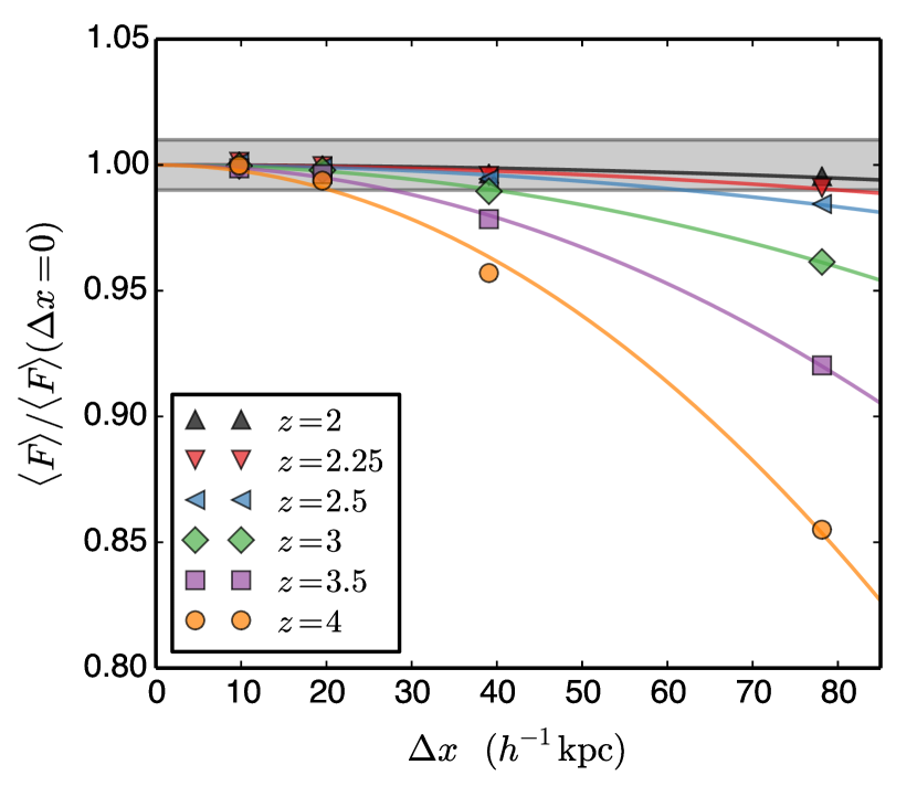
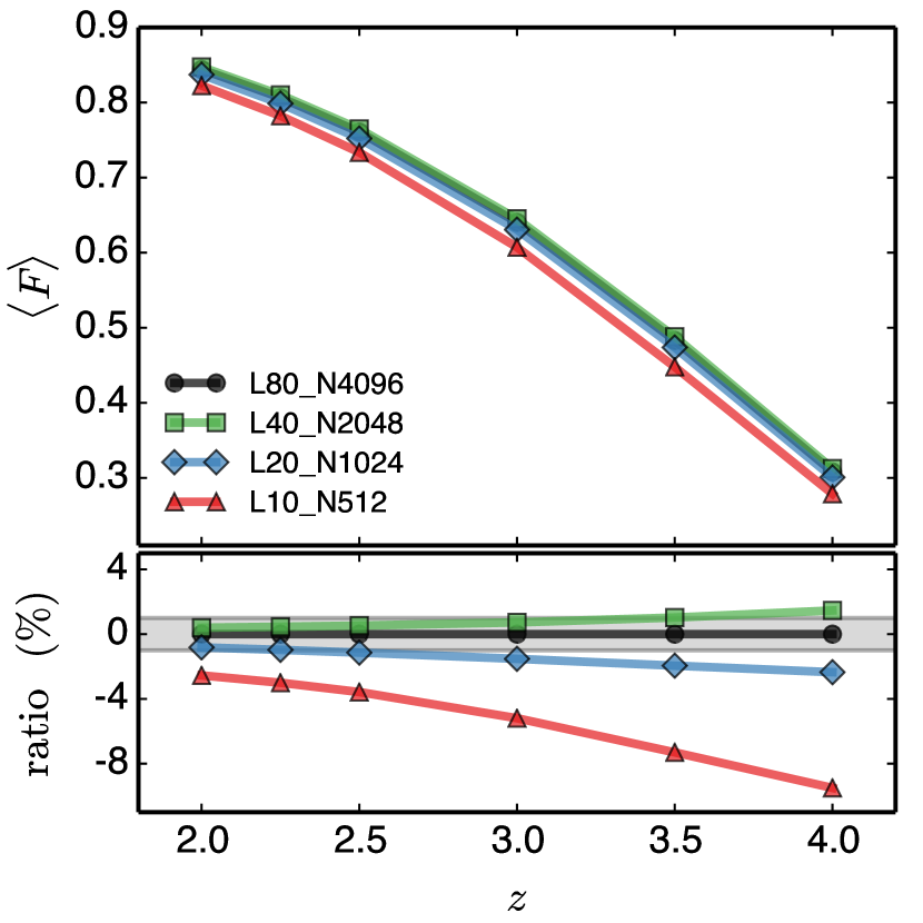
The simplest possible flux statistic is the mean transmitted flux $\langle F\rangle$, or equivalently, the effective optical depth $\tau_{\rm eff}=-\log\langle F\rangle$. Observations show that the mean flux smoothly evolves from about $0.4$ at $z=4$, to about $0.9$ at $z=2$, as expansion gradually lowers the (proper) H i density and the UVB intensity slowly increases (Becker et al., 2013). Figure 9 shows the mean flux in four of our 10 $h^{-1}$Mpc simulations at the snapshot redshifts. Here we immediately see that higher redshifts need higher resolution to maintain the same accuracy. The coarsest resolution run is within 1 per cent of the highest resolution run at $z=2$, but $\sim$15 per cent different at $z=4$. Nyx is second-order accurate in both the gas dynamics solver and gravity. Although the Ly$\alpha$ forest flux is a heavily processed quantity derived from the density, velocity, and internal energy of the gas, its mean clearly exhibits quadratic convergence, as shown in Figure 9. The resolution series allows us to determine $F(0)$ — the simulated mean flux in the limit $\Delta x\rightarrow 0$. Understanding the effect of resolution on the mean flux is important for simulation results that rescale optical depths to match an observed mean flux, as we explore later in Section 7.

4.2 The Flux PDF

The pixel flux probability distribution function (FPDF) is the probability density function of the pixel fluxes (Rauch et al., 1997; McDonald et al., 2000; Becker, Rauch & Sargent, 2007). The probability density function $P(F)$ is defined such that the integral of $P$ over the full $F$ range is equal to 1, $\int P(F)\,dF=1$. In the case of equally-spaced $F$ bins, the $P(F)$ values are just the appropriately rescaled histogram. We compute the FPDF with 50 equally spaced bins of $F\in[0,1)$. The FPDF is a relatively smooth function, with a shape typically peaked at $F=0$ and 1, and rising at intermediate fluxes (although the slope will be negative and there will be no $F\sim 1$ peak at a high enough redshift). In principle this one-point statistic is a good probe of the thermal history of the IGM and the amplitude of density fluctuations, however, the FPDF is very sensitive to systematic effects such as the resolution of the spectrograph, determination of the quasar continuum level and/or pixel noise. Recently, the FPDF was measured using a sample of 3,393 high signal-to-noise BOSS quasar spectra (Lee et al., 2014b), where they found a good fit to the data with a temperature-density slope of $\gamma=1.6$ and strongly disfavoring inverted $\rho$-$T$ models ($\gamma<1$).

Figure 10: Convergence of the flux PDF with respect to grid resolution. For clarity, in the upper panel we have multiplied the $z=2$ data by a factor of 100, and the $z=3$ data by 10.

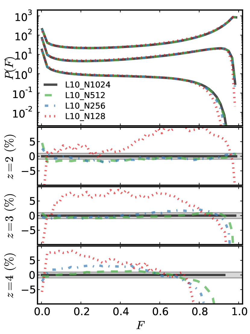
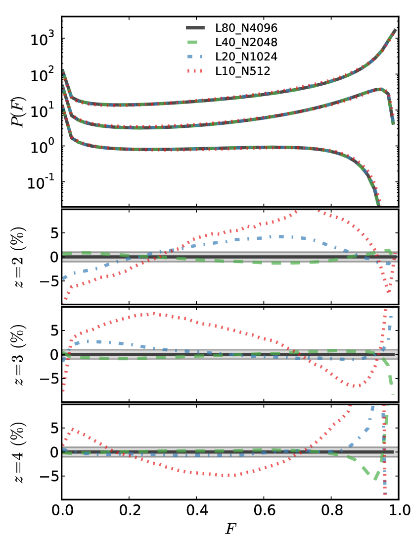
We consider the convergence of the flux PDF $P(F)$ at redshifts 2, 3, and 4, which we show in Figure 10. Again, we note that the resolution requirements increase with redshift. It appears that this is mostly due to the rarity of transmissive regions at high redshift. In the $z=4$ ratio panel, we can see that even the L10_N1024 simulation does not capture pixels with $F\approx 1$, as the black line cuts short near 0.9. It is instructive to look again at Figure 7, which clearly shows how difficult it is to obtain $F=1$ cells at high redshifts, even in very underdense regions. The L10_N512 simulation does match the highest resolution to a few percent up to $F<0.6$. At lower redshifts however, L10_N512 is in percent agreement with the 1024³ run, while the L10_N256 is within a few percent. As expected from the qualitative inspection at the beginning of this section, the L10_N128 simulation results are qualitatively different at all redshifts. At high redshift, it severely underestimates transmissive pixels, pushing the low-flux end above the other simulations. At low redshift, it misses the extreme fluxes at both ends, raising the probability at moderate fluxes above other simulations.

4.3 The 1D Flux Power Spectrum

Figure 11: Convergence of the 1D power spectrum at redshifts 2, 3, and 4. Here we do not modify the values in the upper panel — the flux power increases with increasing redshift, so from top to bottom are redshifts 4, 3, and 2.

Spatial correlations of the Ly$\alpha$ forest offer a promising route to measuring the density fluctuations at high redshifts and small scales. Analogously to density fluctuations, one can define the Ly$\alpha$ forest flux contrast with respect to the mean as $\delta_{F}\equiv(F-\langle F\rangle)/\langle F\rangle$. Here, $\langle F\rangle$ is the global average for a given redshift, but we caution that some older publications use the per skewer mean flux as $\langle F\rangle$. In 3D, the Fourier transform $\hat{\delta}$ and dimensionless power spectrum $\Delta^{2}$ are

$$\hat{\delta}(\mathbf{k})=V^{-1}\int\delta(\mathbf{x})e^{i\mathbf{k}\cdot\mathbf{x}}d^{3}x$$ (11)

$$\Delta^{2}(k)=\frac{k^{3}P(k)}{2\pi^{2}}=\frac{k^{3}}{2\pi^{2}}V\langle\hat{\delta}\hat{\delta}^{*}\rangle$$

where $V$ is the domain volume, $P$ is the power spectrum (in units of volume), and the average $\langle\rangle$ is over shells in $k$-space. In 1D, along the line of sight, the Fourier transform $\hat{\delta}_{\rm 1D}$ and dimensionless power spectrum $\Delta_{\rm 1D}^{2}$ are

$$\hat{\delta}_{\rm 1D}(k_{\parallel})=L^{-1}\int\delta(x_{\parallel})e^{ik_{\parallel}x_{\parallel}}dx_{\parallel}$$ (12)

$$\Delta^{2}_{\rm 1D}(k_{\parallel})=\frac{k_{\parallel}}{\pi}P_{\rm 1D}(k_{\parallel})=\frac{k_{\parallel}}{\pi}L\langle\hat{\delta}_{\rm 1D}\hat{\delta}_{\rm 1D}^{*}\rangle$$

where $L$ is the domain side length, $P_{\rm 1D}$ is the 1D power spectrum (in units of length), and the average $\langle\rangle$ is over modes with magnitude $k_{\parallel}$. The expressions above are written in comoving coordinates $x$ because this is most convenient in simulations. Observationally, however, one measures the flux in velocity units rather than comoving scale, so we also present some results in these units. This creates a small redshift-dependence in the transform between $k$ in comoving coordinates ($h^{-1}$Mpc) and $k$ in velocity coordinates (km^-1 s).

Figure 12: Convergence of the 3D flux power spectrum in 4 $\mu$ bins at redshift $z=4$ (the agreement is better at lower redshifts). The leftmost panel shows the power spectrum mostly perpendicular to the line of sight, the rightmost is mostly parallel to the line of sight. The agreement is better along the line of sight due to thermal broadening which erases some of the differences.

The flux power spectrum is redshift-space distorted and thus anisotropic. But before going into the full anisotropic power spectrum, we will explore its 1D counterpart, obtained by Fourier transforming $\delta_{F}$ along each line of sight and averaging in $k_{\parallel}$ bins. Historically, there were only few a high signal-to-noise quasar spectra which were located far apart from each other. In this limit, individual spectra can be assumed to be independent from each other, and the 1D flux power spectrum is the only relevant measure of flux clustering. Even with SDSS increasing the number of quasar spectra to $\sim 10^{4}$, estimating 3D correlations was still too inaccurate. Today, the main strength of the 1D flux power spectrum is that it can probe relatively small scales, down to $\sim 0.1$ $h^{-1}$Mpc. Therefore, it is a good test of the nature of dark matter and the mass of neutrinos. The observed 1D flux power spectrum has been studied in Croft et al. (1998, 1999); McDonald et al. (2000); Croft et al. (2002); Kim et al. (2004); McDonald et al. (2006); Palanque-Delabrouille et al. (2013).

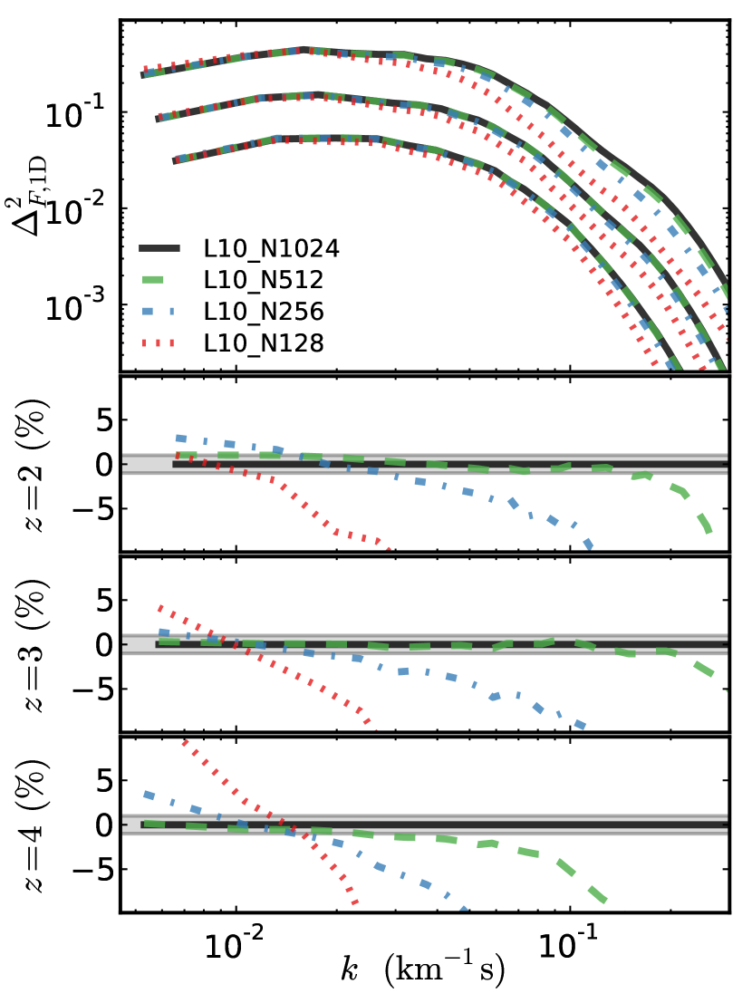
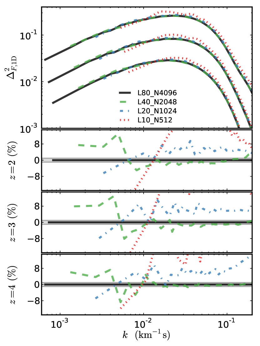
Here we consider the resolution convergence of the dimensionless 1D flux power spectrum $\Delta_{F,\mathrm{1D}}^{2}$ at redshifts 2, 3, 4, as shown in Figure 11, leaving other effects for the subsequent sections. We want to emphasize again that while we show results for the 10 $h^{-1}$Mpc box, we have checked that conclusions are the same in other convergence series in larger box sizes. Figure 11 shows that 20 $h^{-1}$kpc resolution run (L10_N512) agrees with 10 $h^{-1}$kpc run (L10_N1024) to better than 1 per cent at redshifts $z=2$ and $z=3$ even beyond $k=0.1$ km^-1s. Those are much smaller scales than what is usable for making cosmological constrains, as interpreting observations becomes difficult at such small scales due to metal lines and other contaminents. Those scales are also not correctly modeled with the physics included in our simulations. The $z=4$ ratio panel again shows how hard it is to get flux statistics accurately at very high redshifts: the 20 $h^{-1}$kpc run departs from the 10 $h^{-1}$kpc run by 1 per cent around $k=0.03$ km^-1s. This is still sufficiently good for cosmological purposes, especially since the number of observed quasars at such high redshifts is rather small.

One important difference between density and flux fields, is that density is manifestly conserved in our simulations, and its mean value is an input parameter. In contrast, the mean flux will differ — even when the cosmology and physical models for cooling and heating processes are kept constant — due to numerical resolution, box size, and the random realization of the initial density field. Another characteristic feature of the flux field is that it is bounded in value: $0\leq F\leq 1$. The maximum possible fluctuations around the mean value are therefore also limited. This is again in contrast to the density fluctuations, as density contrast can in principle go to infinity. As a result strong suppression of flux fluctuations on small scales — for example due to numerical effects like lack of resolution — results in increased fluctuations on large scales. This effect is also clearly visible in the Figure 11, and is more noticeable when the fluxes in simulations of different resolutions are not rescaled to the same mean (as done here). This effect is the biggest issue to getting the 1D flux power spectrum correct in numerical simulations. Whereas the density power spectrum can, to some extent, be simulated with low resolution simulations using a series of nested-size boxes, each box recovering accurately only a small portion of $P_{m}(k)$, the flux power spectrum in an under-resolved Ly$\alpha$ forest simulation will be inaccurate on all scales.

4.4 The 3D Flux Power Spectrum

Because of redshift space distortions along the line of sight, the 3D flux field is not isotropic, and therefore it is inappropriate to simply average it over $k$ shells as indicated in Equation 11. A common way to describe the anisotropic power spectrum is in terms of the cosine of the angle between the wavevector $\bf k$, and its line of sight component $k_{\parallel}$, $\mu=k_{\parallel}/|\mathbf{k}|$. In other words, the 3D power spectrum is binned in $k$ and $\mu$, rather than $k$ alone, resulting in $P(k,\mu)$. On large scales, the shape of flux power spectrum is very similar to the matter power spectrum (see e.g. Slosar et al. 2009). As such, the Ly$\alpha$ forest is a tracer of the large-scale structure which can measure the characteristics scale of baryon acoustic oscillations (BAO) and use it as a standard ruler to measure the distances and the expansion rate of the Universe. Recently, the first measurements of the cosmological parameters via the location of the BAO peak in the Ly$\alpha$ forest was made with BOSS data (Slosar et al., 2011, 2013; Busca et al., 2013).

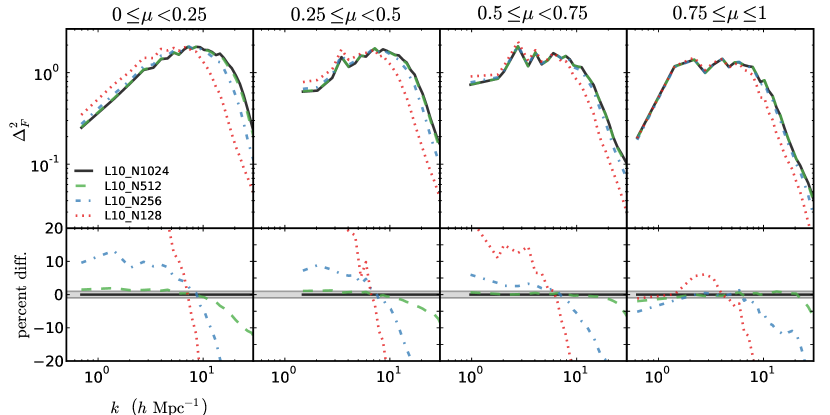
The 3D flux power spectra for 4 $\mu$ bins are shown in Figure 12. The leftmost panel shows the power spectrum mostly perpendicular to the line of sight, and the rightmost is mostly parallel to the line of sight. Here we show only redshift $z=4$ data, since this is where the agreement is worst. The agreement is better at lower redshifts, as expected from previous considerations presented in Sections 2, and 3. We immediately notice that different resolutions agree more along the line of sight than across it. This is a result of thermal broadening which erases much of the small scale differences, bringing the results of lower resolution runs closer to the high resolution solution. We nevertheless see that the 20 $h^{-1}$kpc resolution is good enough for most practical purposes, typically 1 per cent away from the 10 $h^{-1}$kpc result at all redshifts for $k<10$ $h$ Mpc^-1. From the observed rate of convergence we expect that the difference between a 10 $h^{-1}$kpc and a (hypothetical) 5 $h^{-1}$kpc run would be sub-percent.

4.5 Richardson Extrapolation

For a convergent numerical method, it is in principle possible to increase the accuracy of a measured quantity by carefully combining the results from a sequence of simulations where the only difference is the spatial resolution. Here, we discuss the case of combining results via Richardson extrapolation. A numerical method which is $p$-th order accurate in space (meaning the error term is proportional to $h^{p}$ where $h$ is discretization element), produces a numerical approximation $Q(h)$ as

$$Q(h)=Q+Ah^{p}+O(h^{p+1})\ .$$ (13)

The first term on the right-hand side $Q$ is the exact value, the second term is the leading error, and the third term is the higher-order error. The leading error can be removed with simulations using two different values of $h$, for example $h$ and $rh$, where $r$ is the refinement ratio, giving an extrapolation expression

$$Q_{R}=\frac{r^{p}Q(h)-Q(rh)}{r^{p}-1}\ .$$ (14)

The order of accuracy, $p$, is theoretically known from the algorithm implemented, but can also be determined from actual numerical results. This requires at least 3 simulations, in which case $p$ can be calculated as:

$$p=\frac{\ln\left(\frac{Q(r^{2}h)-Q(rh)}{Q(rh)-Q(h)}\right)}{\ln r}\ .$$ (15)

Figure 13: Convergence of 1D flux power spectrum at redshift $z=4$ in a 40 Mpc/h box. We show the results for 512³ and 1024³ simulations, together with the Richardson extrapolation from these two runs using the theoretically expected order of convergence, $p=2$. The shaded band shows $\pm$1 per cent range.

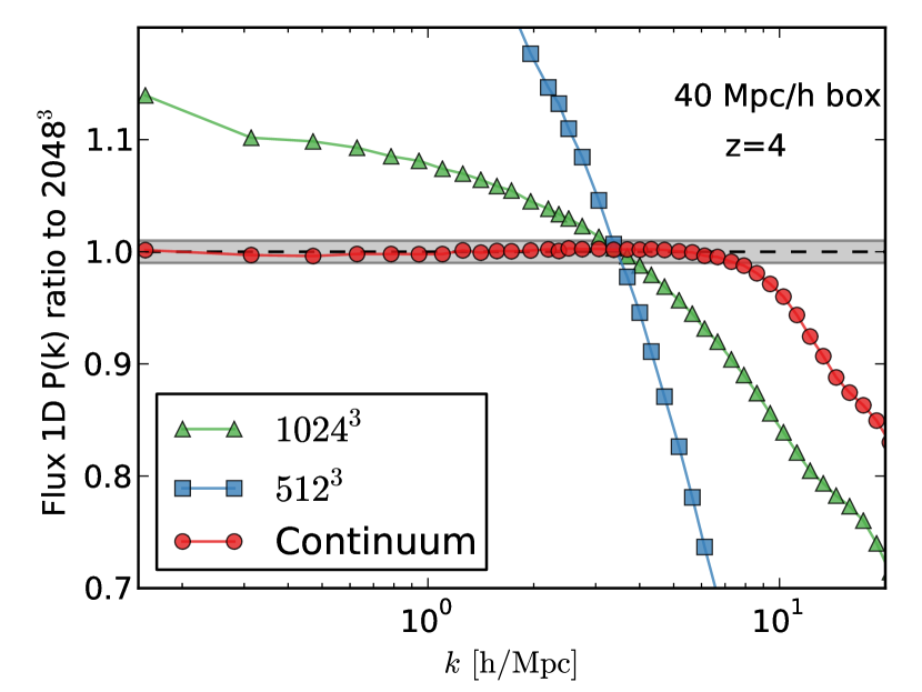
In Figure 13 we show one such Richardson extrapolation, applied to our 1D flux power spectrum results. Here we consider the results at $z=4$, since the differences are largest at this time, and we also use our 40 $h^{-1}$Mpc box size simulations. We see that the run with 40 $h^{-1}$kpc resolution (L40_1024) is not as accurate, differing from the 20 $h^{-1}$kpc resolution run (L40_2048) by up to 15 per cent in the range $k<10$ $h$ Mpc^-1. The run shown in blue (79 $h^{-1}$kpc resolution) — is even worse. However, the “continuum” value deduced from these two runs via Richardson extrapolation, using Equation 14, shows remarkable agreement with the highest resolution reference run. Here, we have used an order $p=2$, since Nyx is formally second-order. The fact that the theoretical value works so well on the 1D flux power spectrum is very reassuring. For larger $k$ values the extrapolation fails. This is expected as the extrapolation procedure cannot reproduce power that is not present in the underlying low resolution simulations, nor can it work in the regime where the convergence breaks down due to a dramatic loss of accuracy close to the resolution limit. Nevertheless, we see that extrapolation can significantly improve accuracy from low-resolution simulations on scales where convergence does hold. This improvement is a strong evidence that numerical errors beyond the discretization scheme Nyx employs are small to none, and a confirmation of the desired rate of convergence even in a very processed quantity like the 1D flux power spectrum.

5 Box Size / Missing Modes

Figure 14: Dimensionless linear and non-linear matter power spectrum at $z=2$. Arrows show the scale of the fundamental mode in our boxes of 10, 20, 40, and 80 $h^{-1}$Mpc.

In cosmological simulations, we model a representative, but finite volume of the universe using periodic boundary conditions in all 3 dimensions. As a result, perturbations on scales larger than the box size are identically zeroed out while fluctuations which are smaller, but comparable to the box size, are poorly sampled. A finite box size can compromise Ly$\alpha$ forest results in at least two different ways. First, in cosmological simulations in general, once the non-linear scale of density fluctuations becomes similar to the box size the evolution of modes is suppressed compared to what would be obtained with a larger simulation box. Second, and relevant to the Ly$\alpha$ forest, a lack of large-scale modes — even linear ones — can lead to an underestimation of the bulk flow velocities of the gas. This, in turn, leads to an underestimation of the heating from accretion shocks. This has a significant impact on both the thermal broadening of lines (via the amount of shock heating) and on the redshift-space distortions of the optical depth. Thus if the simulated box is too small it cannot produce representative Ly$\alpha$ flux statistics for the cosmology of interest.

Figure 15: The matter power spectrum for different box-sizes. We show ratios to the emulated predictions from a gravity-only simulation (Heitmann et al., 2014) at redshifts 2, 3, and 4. Red triangles are 10 $h^{-1}$Mpc box, blue diamonds are 20 $h^{-1}$Mpc, green squares 40 $h^{-1}$Mpc, and black circles 80 $h^{-1}$Mpc box. The resolution is constant in all runs: 19.5 $h^{-1}$kpc.

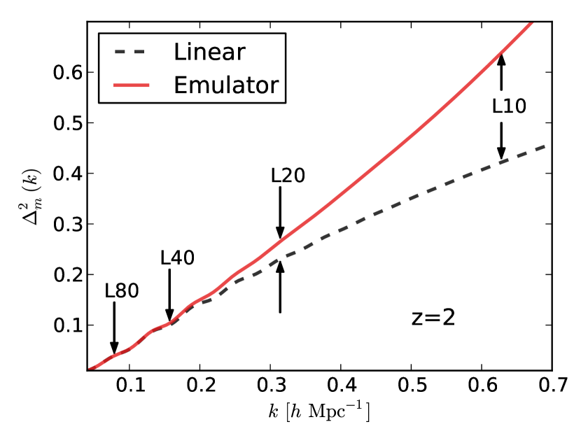
To estimate the non-linear scale of density perturbations, we use the power spectrum emulator FrankenEmu (Heitmann et al., 2014), shown in Figure 14 for the cosmology considered here and at redshift $z=2$. Since we end the simulations at $z=2$, this is the worst-case scenario in terms of the required box size. This alone indicates that 40 $h^{-1}$Mpc is the bare minimum to avoid the box-size mode becoming non-linear, with 80 $h^{-1}$Mpc being a more comfortable value. In the context of “missing modes” in simulations of the Ly$\alpha$ forest, an important and thorough recent work is that of Tytler et al. (2009). The range of box sizes they consider is even larger than the one presented here: their biggest box (54.5 $h^{-1}$Mpc) is similar to our largest, while they go to box sizes as small as 1.7 $h^{-1}$Mpc. Thus most of their simulations are over-evolved at $z=2$, where the largest – anchoring – mode is deeply in the non-linear regime according to Fig. 14. Note that their choice of cosmology has $\sigma_{8}=0.9$, therefore non-linearity starts at even larger scales than the cosmology we consider here. In addition, due to the high computational expense, they had to restrict their box size series analysis to a spatial resolution of 53.3 $h^{-1}$kpc. This resolution is significantly more coarse than the one we find necessary in this paper (20 $h^{-1}$kpc, section 4), but also coarser than what Tytler et al. would have likely run (13.3 $h^{-1}$kpc, see their section 11.3) if it were computationally feasible. Here we present a box size convergence study extending to box sizes large enough to sample linear modes even at the end of the simulations ($z=2$), but also with the desired spatial resolution to capture Ly$\alpha$ statistics to the percent level.

Before turning to flux quantities, we will first look at the convergence of the matter power spectrum in our runs as we increase the box size while keeping the resolution constant. This is shown in figure 15. We clearly see the suppression in mode growth in the small-box simulations with respect to 80 $h^{-1}$Mpc run. The differences in the matter power are rather significant, but as we will show later — and as shown in Tytler et al. (2009) — the differences in the flux power are much less.

5.1 N-Point Statistics

In Figure 16, we show the mean flux in different box-sizes for a constant spatial resolution. As expected, the 10 $h^{-1}$Mpc box is significantly inaccurate, while already in the 20 $h^{-1}$Mpc box we obtain reasonable mean values. As in the resolution study in Section 4, we see the same trend of growing differences as we move to higher redshift. This is not immediately intuitive behavior, as one would expect small boxes to be less affected at $z=4$ rather than at $z=2$. As we do not have many independent realizations of each box-size, we cannot state with certainty how much this effect is due to runs having different realizations versus an actual physical effect. Another thing to note is that convergence is not one-sided (e.g. as the box size is increased the mean flux does not increase as was the case in the resolution study). Again, this could be just statistical variance. Similar behavior is reported in Tytler et al. (2009), see their Table 5. Overall, we see the behavior one would expect from Figure 14 — namely, that there is only a small difference between 40 $h^{-1}$Mpc and 80 $h^{-1}$Mpc boxes. The difference increases with a further reduction in box-size, and becomes clearly too large in the 10 $h^{-1}$Mpc box.

Figure 16: Dependence of the mean flux on the box size, for 6 different redshifts. Upper panel shows the mean flux, lower panel presents the ratio to the largest box-size run – 80 $h^{-1}$Mpc.

As was done in Section 4, we first remove the differences in the mean flux value by rescaling the optical depth in all boxes to the value in our “best” simulation, the 4096³ run in an 80 $h^{-1}$Mpc box. Since the rescaling is small for all but the 10 $h^{-1}$Mpc simulation this plays a rather minor effect, and our conclusions would be the same if we presented unscaled results with the differences being marginally higher. In Figure17 we show the dependence of the flux PDF with respect to the box-size. As in the case of the flux mean, we see that the 40 $h^{-1}$Mpc and 80 $h^{-1}$Mpc boxes are in percent agreement except at the very transmissive end, $F\approx 1$, and at higher redshifts. As commented on in the resolution study, the fully transmissive pixels become very rare at higher redshifts due to the high physical density of neutral hydrogen and therefore the error in determining the relative fraction of such regions decreases. Qualitatively our results at $z=2$ are in line with those presented in Tytler et al. (2009) (though note most of their boxes are smaller than ours).

Figure 17: Convergence of the flux PDF with respect to box size. For clarity, in the upper panel we have multiplied the $z=2$ data by a factor of 100, and the $z=3$ data by 10. The resolution is kept constant at 19.5 $h^{-1}$kpc, and the box-size increases from 10 $h^{-1}$Mpc (dotted red line) to 80 $h^{-1}$Mpc (solid black line).

Next, we turn to the 2-point correlation function of the Ly$\alpha$ forest flux while first examining the 1D $P(k)$. In Figure 18 we immediately see that the differences in the flux power are much less than in the matter power. This is not unexpected as the flux comes from only moderate over densities, which are less affected by the sample variance than halo regions. The convergence of the low-$k$ region is difficult to assess due to different realizations of the initial conditions, but overall we again see nice agreement between the 40 and 80 $h^{-1}$Mpc boxes. Here, however, the 20 $h^{-1}$Mpc box is noticeably in error (by 5-10 per cent) while the 10 $h^{-1}$Mpc box has no value for precision cosmology measurements. As before, our results are in good qualitative agreement with Tytler et al. (2009). As we will show next, most of the differences in the 1D power originate from the differences in power along the line of sight. Despite those differences we conclude that for 1D $P(k)$ constraints the 40 $h^{-1}$Mpc box size is a reasonable one, while 80 $h^{-1}$Mpc is a safe choice.

Figure 18: Convergence of the flux 1D power spectrum with respect to box size at redshifts 2, 3, and 4. Dimensionless flux power is shown in the upper panel, while ratios to the 80 $h^{-1}$Mpc run at 3 different redshifts are shown in the lower panels. Colors and line styles follow that of Figure 17.

Finally, we turn to the 3D P(k), looking at 4 $\mu$ bins, going from across the line of sight $0<\mu<0.25$ to the power along the line of sight $0.75<\mu<1$. This was investigated in McDonald (2003), where they ran simulations with box-size spanning 20 to 80 $h^{-1}$Mpc, very much like the simulations presented here. However, those were HPM simulations rather than full gas dynamics, and the cell size was kept constant at a rather large value of 156 $h^{-1}$kpc.

Figure 19: Convergence of the flux 3D power spectrum with respect to box size in 4 $\mu$ bins. As in Figure12, we show only $z=4$ data, although here this is representative of the agreement at other redshifts as well. The modes at large scales are different due to sample variance.

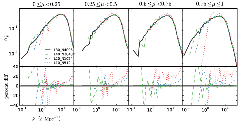
In Figure 19 we see good agreement between the 40 and 80 $h^{-1}$Mpc simulations when the spatial resolution is kept constant. At low $k$, there is a substantial scatter between simulations as random phases in initial conditions differ in different box-sizes. As a result, we cannot meaningfully compare our boxes at large scales. However, at smaller scales, we see that a 40 $h^{-1}$Mpc simulation is in percent-level agreement with the 80 $h^{-1}$Mpc run. Again, just by observing the convergence rate for different box sizes we can be confident that 80 $h^{-1}$Mpc is a very safe value to run at - most likely sub-percent accurate.

Here, we also need to comment on the large-scale Ly$\alpha$ forest bias: on large scales, the Ly$\alpha$ flux is a biased tracer of the matter field, and as such is of great value for cosmology (see Slosar et al. (2011, 2013); Busca et al. (2013)). At present — or in the near future — running hydrodynamical simulations with box sizes needed to sample the BAO peak, and at the same time obtain the resolution necessary to resolve density fluctuations in the IGM, is not a viable approach. Still, one does not necessarily need to have a BAO-regime simulation box to reach a regime where the redshift-space Ly$\alpha$ flux power is related to a real-space density power via a $k$-independent (Kaiser, 1987) formula:

$$P_{F}(k,\mu)=b^{2}(1+\beta\mu^{2})^{2}P_{m}(k)$$ (16)

We have examined bias in our simulations, and have found that they are all too small for a reliable fit to $b$ and $\beta$ of Equation 16. Our 80 $h^{-1}$Mpc box barely reaches a regime where the parameters become scale-independent. Thus, while it is possible to obtain those values using different approaches than directly fitting Equation 16, that work — and especially the comparison with even smaller box-sizes presented here — would be incongruent with the accuracy carried out in the rest of this paper. For now, we will leave it as a separate topic to be carried out in a future work.

6 Splicing

In the previous two sections we have confirmed and quantified both the box-size and resolution requirements for achieving percent-level accuracy for precision Ly$\alpha$ forest cosmology studies. Although possible with today’s high-performance computing facilities, as demonstrated with our L80_N4096 simulation, currently performing a large number of such simulations is impossible. In the past, even a single simulation with that dynamical range was impossible. One technique used to compensate for the lack of dynamical range is splicing, first introduced by McDonald (2003), and most recently employed in Borde et al. (2014). Here we will assess the accuracy of splicing on a 1D flux power spectrum. For completeness, we will first briefly review the method itself.

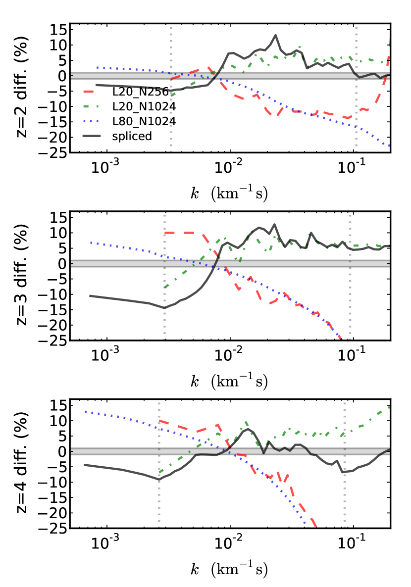
The mechanics behind splicing is to run three simulations, each lacking sufficient dynamic range, and combine them into a result that accurately represents a single full dynamic range simulation. One runs a simulation with enough large-scale power (i.e. a big enough box), but with too coarse a resolution, and another simulation where the box is known to be too small but with good resolution. Finally a simulation is carried out where both resolution and box size are insufficient, the resolution set to the same as in first run, with the box size the same as in the second. The idea is then to use two small-box runs to capture the effect of coarse resolution on the power spectrum, and two runs with coarse resolution to correct for the missing modes in the small-box simulations. Here we will attempt to splice the result of our 4096³ 80 $h^{-1}$Mpc run, which yields percent accurate results as shown via the box-size and resolution convergence tests in the two previous sections. We will thus splice the L80_N1024, L20_N1024 and L20_N256 runs, and compare the result to L80_N4096. Mathematically expressed, in the regime $k<k_{\rm min,20}$, where $k_{\rm min,20}=2\pi/(20\,h^{-1}\mathrm{Mpc})$ the flux power is given as:

$$P(k)=P_{L80\_N1024}(k)\frac{P_{L20\_N1024}(k_{\rm min,20})}{P_{L20\_N256}(k_{\rm min,20})}\,\,,$$ (17)

in the range $k_{\rm min,20}<k<k_{\rm Nyq,80}/4$ where $k_{\rm Nyq,80}=1024\pi/80\,h^{-1}{\rm Mpc}$ is

$$P(k)=P_{L80\_N1024}(k)\frac{P_{L20\_N1024}(k)}{P_{L20\_N256}(k)}\,\,,$$ (18)

and for $k>k_{\rm Nyq,80}/4$ it is

$$P(k)=P_{L20\_N1024}(k)\frac{P_{L80\_N1024}(k_{\rm Nyq,80})}{P_{L20\_N256}(k_{\rm Nyq,80})}\,\,.$$ (19)

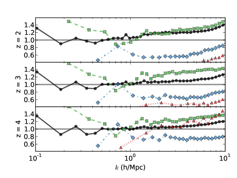
In Figure 20 we show the results of splicing the flux power spectrum at 3 different redshifts. The accuracy of splicing is similar at all redshifts, and is mostly in the $\sim$10 per cent range. That is in agreement with the accuracy estimated by McDonald (2003), but noticeably above the 2 per cent accuracy claimed by Borde et al. (2014). A possible reason for this discrepancy is the fact that Borde et al. (2014) tested the splicing method on a non-converged simulation (1024³ particles in 100 $h^{-1}$Mpc box).

Figure 20: Comparison of a spliced 1D power spectrum and the actual one in a high-resolution, large-box simulation. From top to bottom we have redshift $z=2$, $z=3$, and $z=4$. In addition to the spliced run, we show the ratios of power spectra for each of the three runs used for splicing. All ratios are taken with respect to L80_N4096 run.

7 Rescaling Optical Depths

Up to this point we have ignored the common practice of rescaling the simulated optical depths. In most papers presenting the results of Ly$\alpha$ forest predictions from optically-thin simulations, authors multiply the optical depth in each pixel by some factor $A$ such that the simulated mean flux matches the observed mean flux at the same redshift. This is easily done with any root finding method on $\langle\exp(-A\tau)\rangle-\langle F\rangle_{\rm obs}$ and converges fairly quickly. This fix is well-justified considering how poorly constrained the amplitude, shape, and evolution of the ionizing background are. When we rescale optical depths, it is understood that this is roughly equivalent to adjusting the specific intensity of the UV background used in the simulation. Changes in the photoionization rate, $\Gamma$, in the simulation will most directly affect the H i density while sub-dominant changes will come from photoheating rates. The change in photoheating rate affects the temperature and pressure support of the gas at times when hydrogen or helium are not fully ionized.

Figure 21: Top: Flux statistics from the L10_N1024_HM96 and L10_N1024_FG09 runs at $z=2$. At this redshift, the L10_N1024_HM96 run has $\langle F\rangle=0.8117$, and the L10_N1024_FG09 run has $\langle F\rangle=0.7749$. Also shown are the flux statistics of these runs scaled to the mean flux of the other. Middle: the flux PDF and percent difference compared to the result with the same mean flux. Bottom: the flux 1D power and percent difference compared to the result with the same mean flux.

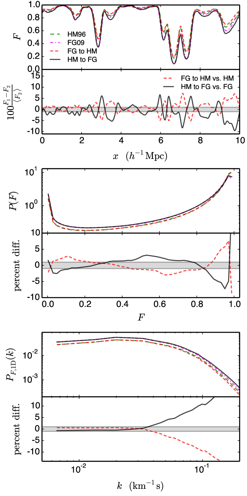
In order to test the effect of rescaling optical depths, we first tried taking two runs with different UV backgrounds (and otherwise the same input parameters) and rescaling one to the mean flux of the other. We used a run with the Haardt & Madau (1996) UVB (labeled L10_N1024_HM96) and a run with the Faucher-Giguère et al. (2009) UVB (labeled L10_N1024_FG09). One concern with starting from different UV backgrounds is that they can result in different $\rho_{\rm b}$-$T$ relations, which would leave differences in the flux statistics no matter how the rescaling is done. The HM96 and FG09 UV backgrounds do result in slightly different $\rho_{\rm b}$-$T$ relations, with very similar slopes but differing $T_{0}$ values. In the case of HM96, we fit $T_{0}=9.0\times 10^{3}$ K and $\gamma=1.55$, and in the case of FG09, we fit $T_{0}=1.1\times 10^{4}$ K and $\gamma=1.55$ at redshift $z=2$. While this is not a significant difference, a temperature difference like this should show up in the flux power spectrum, for instance, as a different thermal cutoff. More importantly, while the two UV backgrounds result in similar instantenious $\rho_{\rm b}$-$T$ relation, the two have significantly different thermal histories: Haardt & Madau (1996) reionizes hydrogen at $z\approx 6$, while Faucher-Giguère et al. (2009) has this occuring at $z\approx 12$. This will result in two UVBs which have a different filtering scale, even if $T_{0}$ and $\gamma$ at a given redshift are the same. At $z=2$, the HM96 run has a mean flux $\langle F\rangle=0.8117$ and the FG09 run has a mean flux $\langle F\rangle=0.7749$. Rescaling the HM run to the FG mean flux requires $A=1.403$ (or conversely rescaling the FG run to the HM mean flux requires $A=0.7138$). We show an example skewer in the top panel of Figure 21. The sample spectrum shows that between the HM96 and FG09 runs the flux in regions of high transmission is similar, but the absorption features are generally deeper in FG09 primarily due to the lower photoionization rate. It is difficult to tell if either run has broader features by looking at just a few lines, but overall we found that the HM96 run does have noticeably broader lines. We also show the spectra after rescaling to the other mean flux. It is reassuring to know that while the correction is an average over the entire box, individual features agree well enough that the correction also works well for individual lines.

The flux PDF and flux 1D power from these runs and their rescaled versions are also shown in Figure 21. In both statistics the HM96 and FG09 results differ by about 30 per cent, but the process of rescaling to the other run’s mean flux brings them to within several percent. The remaining differences in the flux PDF are not straightforward. The rescaled FG09 run has more pixels at low $F$, fewer pixels at intermediate $F$, and more pixels at high $F$ compared to the HM96 result. It appears that the rescaled FG09 rises faster than the HM96 result at $F=0$ and $F=1$. In the 1D flux power spectra, the rescaled versions agree very well at large scales. The rescaled FG09 result has slightly more power than the HM96 result, but it is within 1 per cent. On scales below $k>0.4$ $h$ Mpc^-1, the slopes of the rescaled versions start to diverge significantly. This is due to the differing $T_{0}$ for each, resulting in a different thermal cutoff. Overall, the rescaling process works remarkably well at removing differences from different UV backgrounds, although one should be careful with results that are sensitive to the $\rho_{\rm b}$-$T$ relation.

Figure 22: The evolution of $T_{0}$ for a simulation with Haardt & Madau (2012) UV background (black line), and simulations where photoionization and photoheating rates for all ionic species have been multiplied by the same constant: 1.5 (green line), 2 (blue line), and 3 (red line). Inset panel shows the evolution of $T_{0}$ over the $2\leq z\leq 6$ redshift range.

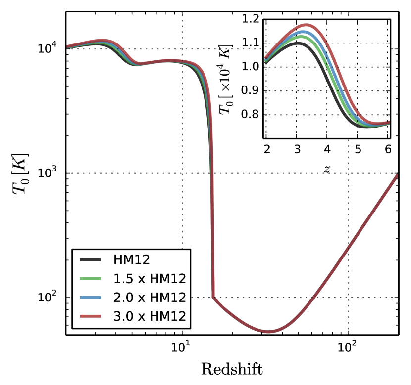
We also made another test of the UVB rescaling, by running simulations where the photoionization and photoheating rates for all ionic species have been multiplied by the same constant. Here we use the Haardt & Madau (2012) rates and, since we multiply all of them by the same factor, the spectral shape of the original UVB is preserved and only the amplitude changes. In figure 22 we show the IGM temperature evolution. As expected modulating the amplitude of the UVB affects the temperature only when a species is not fully ionized. Changes in the hydrogen leave no imprints on $T_{0}$ at observable redshifts, but the same change in helium photoheating rates do change the temperature due to its partial ionization.

Figure 23: The 1D power spectrum from a run using the original Haardt & Madau (2012) UVB rates where the mean flux is rescaled to match that of the run done with doubled UVB rates (2xHM12). We show here the ratio to the actual 2xHM12 run, at 3 different redshifts: $z=2$ (black, squares), $z=2.8$ (blue, circles), and $z=4$ (red, triangles).

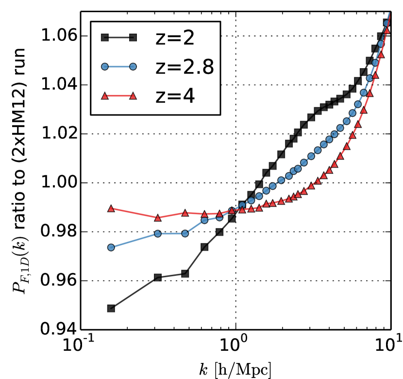
We focus on two runs, one using the original Haardt & Madau (2012) rates, and one where the multiplying factor for all photo-rates is 2, approximately a value needed to recover the observed mean flux in optically thin simulations with this UVB. We compare the run done with doubled photo-rates, labeled 2xHM12, with a flux-rescaled run performed with the original HM12 rates. In other words, the rescaling is done by simply finding the factor $A$ which will bring the mean flux of the original run to that of 2xHM12, a procedure which ignores the differences in the instantenious gas temperature and prior temperature history. The rescaling factor $A$ we recover is close to, but not exactly equal to 0.5, and it shows the tendency to decrease with increasing redshift. For example, it is 1% higher at $z=2$ ($A=0.505)$, than $A=0.5$ at redshift $z=2.4$, and decreases to $A=0.479$ at $z=4$. The results of these rescalings are shown in solid lines in figure 23 for 3 different redshifts. The difference on the 1D power spectrum between rescaling the mean flux and actually running the full evolution with different rates is a few percent, but it is present on all scales. We have also checked the flux PDF, and found smaller differences of approximately 1%. One should note that the difference is smaller at higher redshift, $z=4$, and is the greatest at $z=2$. This means that the effect of different temperature evolutions is more significant for the IGM gas at mild overdensities, and not very significant for underdense gas in void regions.

Figure 24: The percent difference in the 1D flux power spectra between L10_N256 and L10_N1024 at $z=$ 2, 3, and 4, where the optical depths have been rescaled. F- is rescaled to 10 per cent smaller than the L10_N1024 mean flux, F1 is rescaled to same mean flux, and F+ is rescaled to 10 per cent larger. This shows how the convergence rate depends on the mean flux. At $z=2$, the F- power converges fastest, but at $z=3$, the F+ power converges fastest. At $z=4$, the convergence rate is not noticeably affected by 10 per cent changes in the mean flux.

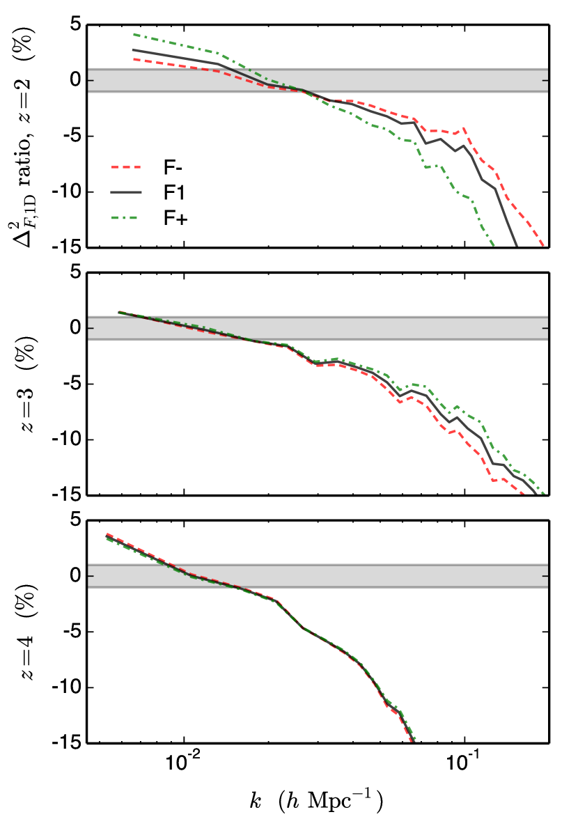
Final test we performed was to take the 10 $h^{-1}$Mpc resolution series runs and test the convergence rate of the flux statistics when changing the mean flux. We compare the flux statistics computed from the same optical depths, but with three rescalings based on the mean flux of the L10_N1024 simulation: one 10 per cent larger, one equal, and one 10 per cent smaller, respectively labeled (F+, F1, and F-). In Figure 24, we show the ratio of 1D flux power spectra between the L10_N256 and L10_N1024 runs, computed from the rescaled fluxes. From top to bottom, we show the result for $z=2$, 3, and 4. At $z=2$, we see that the 1D power converges faster for a lower mean flux. The resolution error in the 1D flux power shows a characteristic slope difference (the lower resolution result has a more negative slope), and at $z=2$, the slope difference is smallest for the lower mean flux rescaling, and largest for the higher mean flux rescaling. Rescaling flux to a lower mean value means shifting flux contributing regions to lower gas density, or equivalently less nonlinear structures, and thus it is easier for a simulation to be converged. At $z=3$, we see the opposite trend, that the results converge faster with a higher mean flux rescaling. This indicates a “sweet spot” mean flux (or similarly, a redshift) where it is easiest to resolve Ly$\alpha$ forest structures. When the mean flux is very high, the forest probes higher densities closer to halos which are harder to converge. Similarly, when the mean flux is very low, the forest has significant sensitivity to the very underdense regions. Although we are examining purely numerical effects here, note that these conclusions also translate to the question of the importance of additional physics in simulations. From what we have presented in this section, one would clearly expect galactic outflows, AGN feedback, and other processes originating within galaxies to matter much more at e.g. redshift $z=2$ than $z=3$. At $z=4$, we see no difference in the convergence rate with the different mean flux rescalings. At this high of a redshift, the mean flux is low and a rescaling of only $\pm 10$ per cent does not significantly affect the density range contributing to the forest (see the red bands in Figure 7).

Finally, another issue with the practice of rescaling to the observed mean flux is that few current Ly$\alpha$ forest simulations are converged to the percent level in $\langle F\rangle$ at high redshift. As shown previously, even simulations with a resolution of $\sim 40$ $h^{-1}$kpc are not converged to a percent in the mean flux for $z>3$. Taking a simulation of insufficient resolution and performing a mean flux rescaling will result in the wrong correction. Under-resolving IGM structures results in a mean flux lower than it should be, so a rescaling to a higher mean flux, for instance, will require a smaller rescaling factor $A$ than what would be needed for a higher-resolution run.

8 Small Scale Statistics

8.1 Line Statistics

The Ly$\alpha$ forest is classified as systems with $N_{\textrm{H}\,\textsc{i}}<10^{17}$ cm^-2, known for sitting in the linear portion of the curve of growth. This makes it straightforward to fit the Ly$\alpha$ forest lines with Doppler profiles. Each line fit provides the column density $N_{\textrm{H}\,\textsc{i}}$ and Doppler parameter $b$ of the underlying system. However, this neglects the issues of significant line blending in the forest, as well as line broadening dominated by Hubble broadening rather than thermal broadening. Meiksin, Tittley & Brown (2010), for instance, mention that line shapes in simulated spectra ignoring peculiar velocities are qualitatively different than those in the full spectra. This indicates that the $N_{\textrm{H}\,\textsc{i}}$ and $b$ derived from line fitting may not correspond to the actual column density and temperature distributions of the gas that makes up the forest. However, line parameter distributions are a sensitive measure of line shapes in the forest. Additionally, interpreting line parameter statistics is fairly straightforward — the column density is a proxy for equivalent width and the Doppler parameter is the line width.

Figure 25: The distributions of the line H i column density (left) and the Doppler parameter (right) in the resolution series of the 10 $h^{-1}$Mpc boxes at $z=2$. The percent difference relative to the L10_N1024 simulation is shown in the bottom panels. In the $P(N_{\textrm{H}\,\textsc{i}})$ panel, the gray line illustrates the power law slope $\propto N_{\textrm{H}\,\textsc{i}}^{-1.6}$. In the $P(b)$ panel, the thin dashed red and black lines show lognormal distribution fits to the L10_N128 and L10_N1024 results, and the red and black text gives the corresponding median $b$-parameter values (also the peak probability). The simulated $b$-parameter distributions are more skewed than lognormal, but a lognormal fits the core of the simulated distributions well.

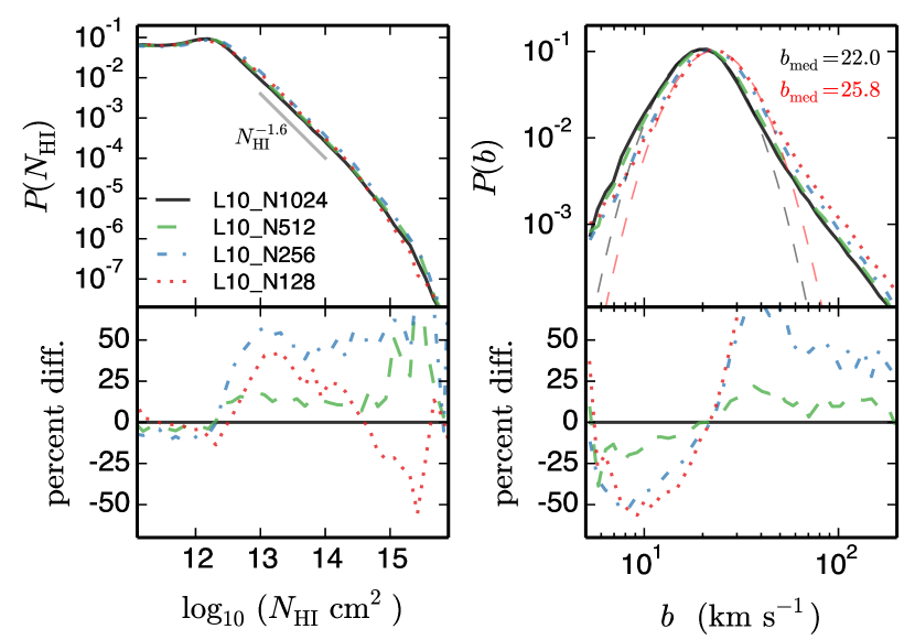
In this work, we generate spectra with a fixed resolution of $\Delta v_{\rm pix}=1$ km/s to avoid possible issues of the fits depending on spectral resolution and the assumed pixel SNR. We have chosen this resolution because it is sufficiently smaller than what we expect for the minimum line width of gas at $T=10^{3}$ K, which corresponds $b=4$ km s^-1 for hydrogen. We want to reduce statistical uncertainty in the distributions as much as possible, which means having many lines in each bin. The line compilation in Haardt & Madau (2012) (their section 3), provides $dN/dz$ of systems above a given $N_{\textrm{H}\,\textsc{i}}$. At $z=3$, $dN/dz=24.2$ for $N_{\textrm{H}\,\textsc{i}}>10^{15}$ cm^-2. The corresponding path length required to find $10^{4}$ absorbers (for 1 per cent statistics) is $2.9\times 10^{5}$ $h^{-1}$Mpc, or a total spectral length of about $3.1\times 10^{7}$ km s^-1. The L10_N128 simulation is actually smaller than this, so we use the entire box in that case. For all other runs, we evenly distribute the skewers throughout the volume up to the required path length. We use the specfit code (first used in Meiksin, Bryan & Machacek, 2001) to perform the Voigt line fitting of our simulated spectra. For each spectrum, the code splits the spectrum into regions separated by a threshold value $\tau>\tau_{\rm min}$. In these absorption regions, specfit uses first and second derivatives of the flux to identify line centers and then performs a $\chi^{2}$ minimization of the line parameters.

We show the effect of simulation resolution on the line parameter distributions in Figure 25. We show the probability distribution function of the line column density in the range $11<\log_{10}(N_{\textrm{H}\,\textsc{i}}\,\mathrm{cm}^{2})<16$ and the Doppler parameter in the range 5 km/s $<b<$ 200 km/s and the percent difference to the L10_N1024 results. The column density distribution is relatively flat for $N_{\textrm{H}\,\textsc{i}}<10^{12.5}$ cm^-2, and then turns over to a power law $dN/dN_{\textrm{H}\,\textsc{i}}\propto N_{\textrm{H}\,\textsc{i}}^{-1.6}$, where the slope of the power law depends on the UV background. The annotated gray line gives an example of the power law slope. Qualitatively, the different resolutions agree well. The L10_N128 and L10_N256 runs do not peak as much at $N_{\textrm{H}\,\textsc{i}}<10^{12.5}$ cm^-2, and turn over more slowly, resulting in an excess probability of lines in the $12.5<\log_{10}(N_{\textrm{H}\,\textsc{i}}\,\mathrm{cm}^{2})<14$ range. This same trend is present in the L10_N512, but it is less significant. The lowest resolution run, L10_N128, shows a deficit of high column density lines $N_{\textrm{H}\,\textsc{i}}>10^{14}$ cm^-2 compared to the other runs. The Doppler parameter distribution is close to lognormal with a peak around $b=20$ km/s. The Doppler parameters distributions show a much clearer convergence pattern. The overall shape of the Doppler parameter distribution does not appear to change with resolution, but the peak $b$ value decreases with increasing resolution. This holds together with our qualitative picture of the resolution study – the lower-resolution runs are like artificially smoothed higher-resolution runs, so the resulting absorption lines are broader as well. We also show two fits of the lognormal distribution $P(b)=A/(b\sigma)\exp[-(\log b-\log b_{\rm med})^{2}/(2\sigma^{2})]$, where $A$, $b_{\rm med}$, and $\sigma$ are the free parameters. The red thin dashed line is the fit to the L10_N128 and the black thin dashed line is the fit to the L10_N1024 result. From the lowest resolution to the highest resolution result, the median $b$ value changes from 25.8 km/s to 22.0 km/s, and the corresponding temperatures are $3\times 10^{4}$ K and $4\times 10^{4}$ K. This is an important consideration for studies using small-scale statistics to infer the temperature of the IGM. If we were to use the low-resolution runs to infer the IGM temperature, we would be biased to lower temperatures than results based on higher-resolution runs (the fit $T_{0}$ values are essentially the same in these runs).

Figure 26: The distributions of the line H i column density (left) and the Doppler parameter (right) in the box size series with a grid scale of 20 $h^{-1}$kpc at $z=2$. The percent difference relative to the HM12_L80_N4096 simulation is shown in the bottom panels. In the $P(N_{\textrm{H}\,\textsc{i}})$ panel, the gray line illustrates the power law slope $\propto N_{\textrm{H}\,\textsc{i}}^{-1.7}$.

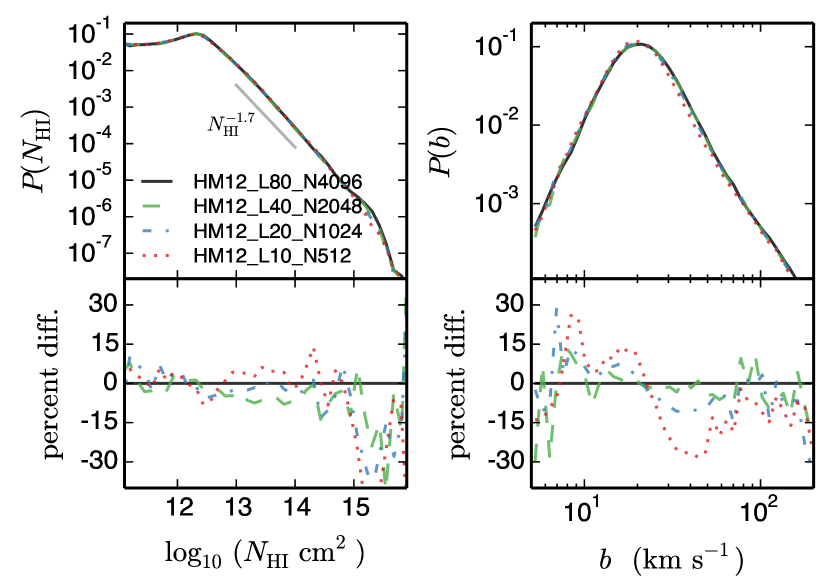
We show the effect of simulation box size on the line parameter distributions in Figure 26. Compared to the resolution series, the box size has little effect on the line fits. The different UVB in the box series simulations results in a slightly steeper $N_{\textrm{H}\,\textsc{i}}$ distribution power law, shown with the gray line matching $\propto N_{\textrm{H}\,\textsc{i}}^{-1.7}$. The column density distributions across box size are very close to each other, and differences appear to be in the statistical noise. More significant differences appear above $N_{\textrm{H}\,\textsc{i}}>10^{15}$ cm^-2, however, this is also mostly due to the rarity of well-fit high column density systems. The box size has a clearer effect on the Doppler parameter distribution, although it is still much smaller than the resolution effect. Again, the distribution shape across box size is essentially the same, but the peak position increases with increasing box size. This is hard to see in the top $P(b)$ panel, but in the bottom difference panel, we see the curves flattening out around $b=20$ km/s with increasing box size.

8.2 Wavelet Statistics

Figure 27: Convergence of the flux discrete wavelet transform power with respect to physical resolution in 10 $h^{-1}$Mpc box.

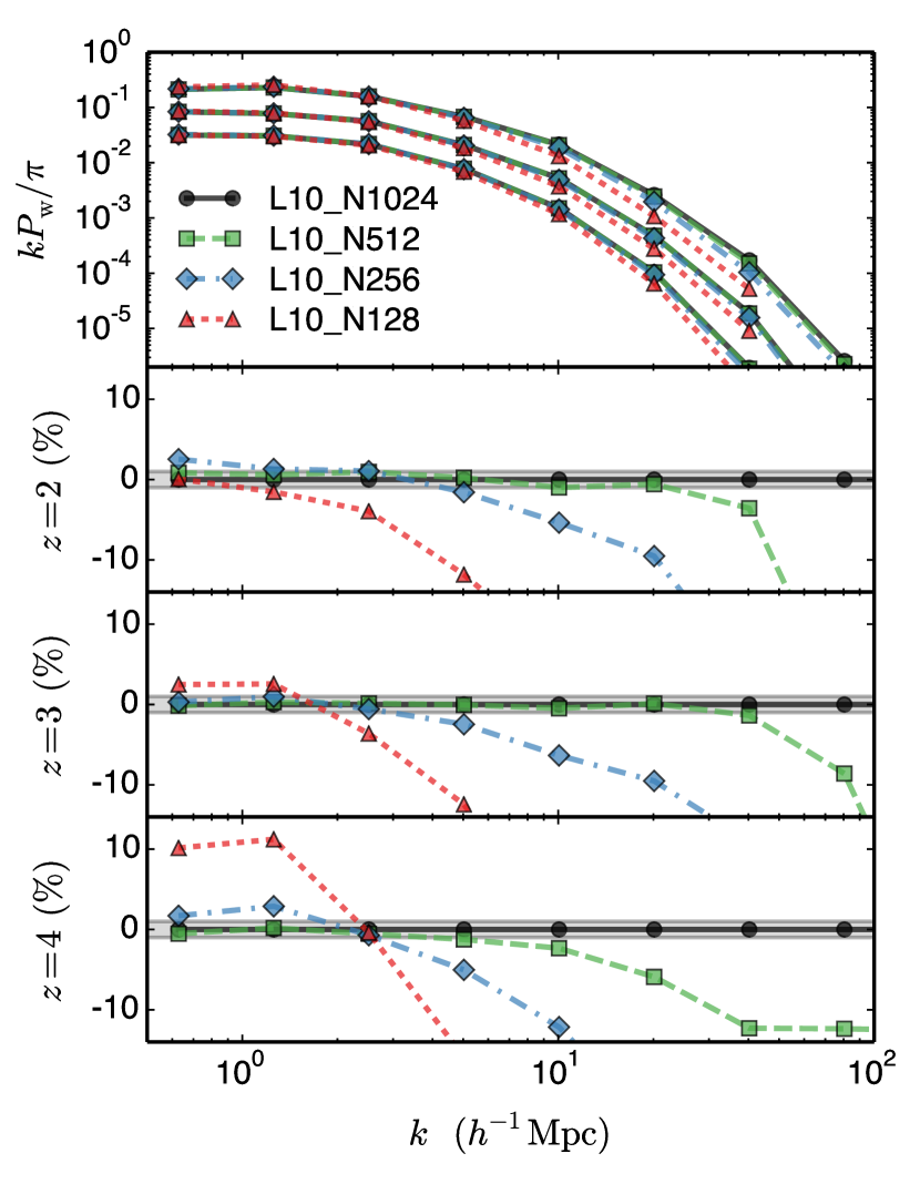
In addition to line fitting, we also performed a wavelet power analysis of our spectra. Wavelets have previously been applied to the Ly$\alpha$ forest as a means of objectively measuring the line widths, primarily in order to probe the IGM temperature. Meiksin (2000) introduced wavelets as a tool for the Ly$\alpha$ forest as a means of data compression and a measure of small-scale power. Zaldarriaga (2002) extended the use of wavelets to search for spatially localized line-width (temperature) fluctuations, an analysis recently repeated with a slightly different use of wavelets in Lidz et al. (2010) and Garzilli et al. (2012). Theuns et al. (2002) used wavelets to search for temperature fluctuations in the IGM associated with He ii reionization.

Wavelet basis functions are orthogonal and complete, providing well-defined transforms into wavelet coefficients and back. More importantly, wavelets are localized in real and Fourier space. The discrete wavelet transform (DWT) is a decomposition of some signal $f$ into discretized wavelet bases $\psi_{jk}(x)$, where we use $j$ as the level (sometimes called stretch) of the wavelet and $k$ as the shift (or position). The DWT provides wavelet coefficients $w_{jk}$ such that $f(x)=\sum_{j,k}w_{jk}\psi_{jk}(x)$, and in this case we are transforming the flux fluctuations $\delta_{F}$ along the line of sight. We use the Daubechies 20 coefficient wavelet, which is the most common choice for wavelet analysis. With the wavelet coefficients in hand, we can compute the wavelet power spectrum $P_{\rm w}$ as average of the squares of the coefficients, just as one would with Fourier coefficients.

$$P_{\rm w}(k_{j})=L\langle w_{jk}^{2}\rangle$$ (20)

where the average is taken over all of the shifts $k$ for the level $j$. The $L$ factor is included to match our previous Fourier convention and the dimensionless wavelet power spectrum is $k_{j}P_{\rm w}/\pi$. We associate the level $j$ to the mode $k_{j}=2\pi/L2^{j-1}$.

Figure 27 shows the impact of spatial resolution on the wavelet power. As expected, we see very similar behavior to the flux power spectrum, namely the percent level agreement between the 20 $h^{-1}$kpc (L10_N512) and 10 $h^{-1}$kpc (L10_N1024) runs. As with the power spectrum we see that inadequate resolution to capture the fluctuations responsible for the rise of the Ly$\alpha$ forest produces an error on all scales, not only scales below the resolution limit. We have checked that the box-size behavior is also very similar to that seen in $P_{F}(k)$, Figure 18.

9 Collisionality

In order to obtain a correct distribution of Ly$\alpha$ spectral lines it is essential for simulations to correctly capture the temperature of the IGM for a given physical and cosmological model. That is the reason we opt here to use a highly accurate shock capturing scheme for gas dynamics. In this section we investigate the potential artificial heating of the IGM gas due to the numerical collisionality of dark matter particles. Steinmetz & White (1997) have shown that the discretization of dark matter particles gives rise to a steady flow of energy from dark matter to the gas. In their paper, they both outlined the analytic theory for the artificial heating of the gas, and tested it in both the adiabatic case and in the presence of radiative cooling – a regime of interest here. The focus of their study was dense regions, galactic-size halos, where this effect is expected to be smaller than in the low-density IGM. A particular concern for us is that there is a non-negligible contribution to the Ly$\alpha$ forest from regions which are quite underdense, i.e. where we have less than 1 particle per cell in our runs. We are further sensitive to this error due to our code’s ability to capture and propagate weak shocks indiscriminate of whether their origin is physical or numerical. It is therefore important to consider and quantify this numerical source of gas heating.

Figure 28: Left: A slice of dark matter density from L10_N512 simulation (1 particle per cell). Middle: A slice of dark matter density with 8 particles per cell (1024³ particles on a 512³ grid). Right: The PDF of dark matter from both runs. We have used a Cloud-In-Cell method to deposit particles on the grid, a common approach in cosmological simulations.

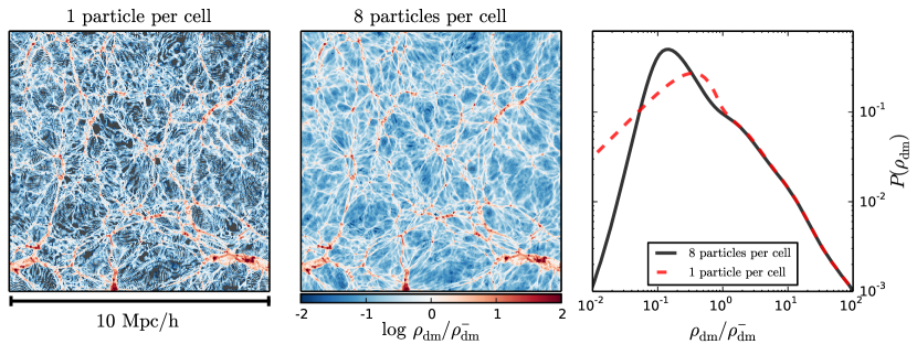
Here we take our L10_N512 run to be “the fiducial” one, as it has one particle per cell, a common value encountered in Ly$\alpha$ forest simulations. This roughly corresponds to runs with the same number of particles for dark matter and gas particles in SPH simulations, which is typical of almost all SPH simulations in the literature. We compare this run with 512³ particles, with a run done on the same grid, with the same code parameters and cosmological realization, but with 1024³ particles. Figure 28 shows a slice of dark matter in both runs together with the PDF from the whole box. We clearly see the discretization error the Cloud-in-Cell method introduces to underdense regions. Here there is a clear transition at one particle per cell with those at higher densities performing well while those lower than this inaccurately estimating the dark matter densities. We have also checked the PDF of the baryon densities in the two runs, and confirmed that differences are less than 1%. In void regions, where the dark matter density is least correctly represented on the grid, the evolution of matter is driven by the large-scale gravitational field, therefore the sampling of the dark matter on the grid scale does not significantly alter the distribution of baryons directly, other than via pressure forces due to the change in gas temperature.

Our numerical simulations show that the effect of collisional heating in the gas is indeed present, but overall it is negligible. We do not observe a significant change in the gas temperature as shown in Figure 29. Here, we show the median difference between the two runs over the density range relevant for the Ly$\alpha$ forest, along with the median absolute deviation scatter (defined as the median of the absolute deviations in temperature of each cell from the full-box temperature median, scaled to give 1$\sigma$ for a Gaussian distribution). The differences in the median are within 1 per cent throughout this density range while the MAD scatter increases with density. The latter is at least partially an artifact of sampling, as the number of cells decreases with increasing density (recall Figure 3). Even in void regions, cell-to-cell comparisons shows less than a percent difference – thus the effect of artificial collisionality is small. The fact that the scatter goes negative shows that some cells are cooler in the run with coarser dark matter particle mass. It is likely an indication that other discretization effects (the deposition of particles and the addition of gravitational force in the Euler equations) introduce at least the same amount of error as collisional heating.

As a result, we observe that the difference in flux statistics is small, less than 0.5 per cent in the flux PDF, and less than 1 per cent for the 1D power spectrum up to $k=10$ $h$ Mpc^-1. This is below the level we are presently concerned with in making theoretical Ly$\alpha$ forest predictions. Note that the small effect particle sampling plays is not completely unexpected: simulations focusing on the IGM suffer from coarse particle sampling in the relevant regions, but the mass of dark matter particles is still small enough in today’s simulations. Therefore the (real) radiative cooling still dominates over the (artificial) collisional heating process.

10 Conclusions

We have investigated simulated Ly$\alpha$ forest statistics over the redshift range $2\leq z\leq 4$. A large suite of simulations covering box sizes of 10-80 $h^{-1}$Mpc, and resolutions 10-78 $h^{-1}$kpc have enabled us to understand the numerical requirements for future sets of simulations aimed at constraining cosmological parameters using the Ly$\alpha$ forest. While we model gas dynamics using a very accurate finite-volume numerical method, the additional physics which enters as a source (heating) term in the energy equations as well as those used to calculate the ionization state of a primordial chemistry gas is accounted for in a more approximative way. In our optically thin simulations, the gas is rapidly ionized by the assumed UVB at high redshift, and in a short time changes its ionization fraction by order unity – a model of sudden reionization. We neglect the effects of self-shielding in high over-density regions as those do not contribute to the Ly$\alpha$ forest signal. The temperature boost during the sudden reionization depends only on the shape of the spectrum of ionizing radiation, and in fact one expects a range of spectral shapes responsible for ionizing different gas elements. Modeling the details of temperature evolution during and immediately after reionization requires full radiative transfer simulations and is beyond the scope of our needs here, as the thermal memory of the IGM gradually fades after the epoch of reionization (mostly due to Compton cooling, see Hui & Gnedin 1997).

As the IGM fills the simulation box, it is fruitless to try to resolve it with adaptive refinement; similarly, as a large portion of the Ly$\alpha$ forest signal arises from near mean and under-dense regions (especially at at higher redshifts), Lagrangian methods do not offer any advantage over a fixed grid PDE solver. Needless to say the fixed grid approach is computationally expensive, especially in the 3D case presented here, and thus it is important to determine the minimal resolution requirements needed to bring our simulations to 1 per cent accuracy. We have explored this in section 4 arriving at the conclusion that $\sim 20$ $h^{-1}$kpc resolution is good enough over the relevant redshift ranges we wish to consider for the Ly$\alpha$ forest. While in places — for example the flux PDF — a coarser resolution would suffice, the study of 1D power spectra brings with it a more stringent requirement. While we explored resolution convergence, we were also able to show that Nyx behaves well on this multi-dimensional, multi-physics problem, exhibiting the expected second order convergence. As shown in section 4, this opens the possibility of achieving a desired accuracy at reduced cost, via extrapolation of lower-resolution runs.

We also explored other numerical artifacts which can easily mask a physical process in the IGM and/or spoil the quality of cosmological predictions. After finding an appropriate resolution, we have explored the effects of finite box-size, i.e. missing modes in Ly$\alpha$ forest simulations. By running simulations with all cosmological and numerical parameters but the box-size fixed, we were able to show that 40-80 $h^{-1}$Mpc boxes are large enough for all relevant statistics including the 3D power spectrum in redshift space, i.e. $P(k,\mu)$. For the first time, we were able to perform a Ly$\alpha$ forest simulation fulfilling both the resolution requirement set by the Jeans / filtering scale and the box-size requirement set by large-scale flows. That enabled us to examine the accuracy of splicing 1D power spectra, a common approach in the case when a full range of simulations are not feasible (McDonald, 2003; Borde et al., 2014). We show that accuracy of splicing is only 5-10 per cent, and that the error has a clear scale-dependence.

Figure 29: Change in the gas temperature in a standard run with 1 particle per cell ($T_{1}$), and an “overloaded” run with with 8 particles per cell on average ($T_{8}$). The line shows the difference in the median temperatures and the fill shows the normalized median absolute deviation in temperatures. The median deviation is roughly symmetric and the resulting effect on the Ly$\alpha$ forest statistics is negligible. In addition, we show statistical (Poisson) errorbars in each density bin.

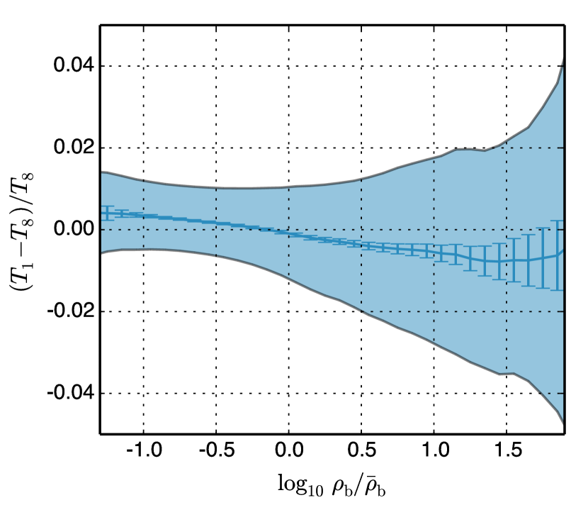
As the UV background is the largest uncertainty in Ly$\alpha$ forest simulations, it is very common that a cosmological model is evolved with a UVB model, with the resulting optical depth field subsequently rescaled to match desired, observed mean flux value. In Section 7, we examined the effects of changing the UVB and rescaling the mean flux. We found that while qualitatively it is possible to change the UVB post festum in analysis, one suffers a few percent effect in the UVB rates propagating back into the gas evolution which is most visible in the flux PDF. We note that the 1D $P(k)$ appears largely insensitive to such rescaling for $k\lesssim 3\times 10^{-2}$ km^-1s, the $k$-range relevant for current observational data.

We find that resolution requirements for convergence on the line statistics are much more demanding than on the flux statistics. A resolution of 20 $h^{-1}$kpc, adequate for reproducing the flux statistics to 1 per cent accuracy as shown in section 4, recovers the distribution of neutral hydrogen column densities only at $\sim$10 per cent accuracy in the range $12.5\lesssim\log_{10}(N_{\textrm{H}\,\textsc{i}}\,\mathrm{cm}^{2})\lesssim 15$, and even worse at higher column densities. Similarly, the Doppler parameter ($b$) distribution is converged at the same level, with the peak value decreasing with increasing resolution. This is not directly relevant to modern cosmological studies which do not rely on individual line fitting, but it is important for certain studies of the IGM.

Finally, we have explored the effects that finite sampling of the dark matter particles has on the statistics of the Ly$\alpha$ forest. The expectation is that artificial gravitational collisionality between dark matter particles and gas increases the gas temperature, an effect that should be strongest in void regions. While we indeed notice, on average, temperature increases in void regions, the effect is minor in today’s simulations even when using 1 particle per cell and CIC particle deposition. The reason for this is the small particle mass in Ly$\alpha$ forest simulations and the presence of radiative cooling, which efficiently removes excess heat.

The advent of high performance computing power and scalable numerical algorithms as employed in Nyx allows us to make accurate predictions for the Ly$\alpha$ flux statistics, one of the most promising tools for precision cosmology measurements in the redshift range $2\lesssim z\lesssim 4$. The direct simulation approach, using no ad hoc physical assumptions, is possible for this problem. We have made a concentrated effort here in understanding the Ly$\alpha$ forest signal in optically-thin hydrodynamical simulations, and quantifying the accuracy of such simulations with respect to numerous numerical effects. We are by no means the first to attempt this (indeed they go back at least to Cen 1992), however we have been able to consolidate and improve upon earlier studies using modern simulations with the goal of percent-level numerical precision, a level of accuracy required for carrying out precision cosmology over the next decade.

We note that full-range, $4096^{3}$, hydrodynamical simulations like the one presented in this paper are still computationally demanding today, but will be a fairly typical in coming years. Before one commits to running many such simulations, it is imperative that the precision which can be obtained be understood. Convergence testing is an invaluable tool here, as analytically soluble problems are highly artificial in nature, and experience with them does not necessarily translate to real cosmological runs. In our paper we have used the Nyx code. While Nyx is focused on Ly$\alpha$ forest simulations, the results presented here should be directly applicable to IGM simulations performed by the Enzo, Flash and Ramses codes. In addition, there are several lessons applicable to a large extent to the Gadget and Arepo codes as well. In a future work (Stark et al., 2014) we will compare SPH and Eulerian methods for simulating the Ly$\alpha$ forest.

Appendix A Atomic Rates

Figure 30: Top: A comparison of different hydrogen recombination rates used in recent simulations in the literature and Verner & Ferland (1996) calculated data. Bottom: Comparison of photoionization rates published in recent works: solid lines are Haardt & Madau (2012), and dashed lines are Faucher-Giguère et al. (2009) (revised in Faucher-Giguère, Kereš & Ma 2011).

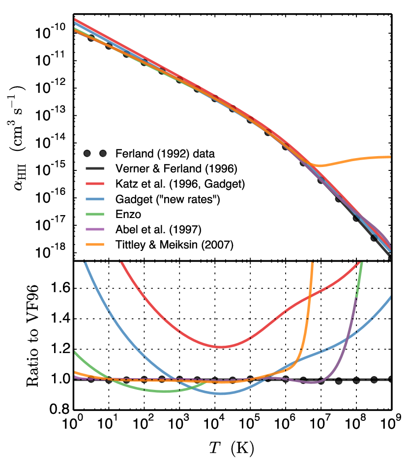
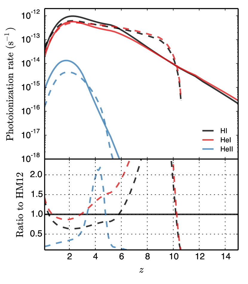
Here we provide some details on the reaction rates implemented in the Nyx code. In order to provide an easy comparison to the Gadget code, we have also implemented the atomic rates from Katz, Weinberg & Hernquist (1996). Some of the runs presented in this paper use those rates, as well as a companion comparison study between Nyx and Gadget (Stark et al., 2014). However, we also implement more accurate rates which will be used in future Nyx studies exploring cosmological effects in Ly$\alpha$ forest statistics. These are also used here for our biggest 4096³ run and the accompanying smaller runs used in the box-size study in Section 5. These rates are shown in Table 3, along with their references.

We explicitly keep track of the net loss of thermal energy resulting from atomic collisional processes. Those rates are shown in Table 4. In addition to the tabulated cooling rates, Nyx includes cooling from inverse-Compton scattering off CMB photons as in Peebles (1968)

$$L_{C}=\frac{4\sigma_{T}ak_{B}}{m_{e}c}n_{e}T^{4}_{\rm CMB}(z)\left[T-T_{\rm CMB}(z)\right]\,,$$ (21)

where $\sigma_{T}$ is the Thomson cross section, $a$ is the radiation density constant, $k_{B}$ is the Boltzmann constant, $m_{e}$ is the electron mass, $c$ is the speed of light, and $T_{\rm CMB}$ is the temperature of the microwave background, which we take to be $T_{\rm CMB}=2.725$.

Table 3: Atomic rates in Nyx

Coefficient	Fitting formula [${\rm cm^{3}s^{-1}}$]	Comment
	$a\left[\sqrt{T/T_{0}}\left(1+\sqrt{T/T_{0}}\right)^{1-b}\left(1+\sqrt{T/T_{1}}\right)^{1+b}\right]^{-1}$	Verner & Ferland (1996)
$\alpha_{\rm r,\textrm{H}\,\textsc{ii}}$	$a=7.982\times 10^{-11}$, $b=0.7480$, $T_{0}=3.148$, $T_{1}=7.036\times 10^{5}$
$\alpha_{\rm r,\textrm{He}\,\textsc{ii}}$	$a=3.294\times 10^{-11}$, $b=0.6910$, $T_{0}=15.54$, $T_{1}=3.676\times 10^{7}$	$(T\leq 10^{6})$
$\alpha_{\rm r,\textrm{He}\,\textsc{ii}}$	$a=9.356\times 10^{-10}$, $b=0.7892$, $T_{0}=4.266\times 10^{-2}$, $T_{1}=4.677\times 10^{6}$	$(T>10^{6})$
$\alpha_{\rm r,\textrm{He}\,\textsc{iii}}$	$a=1.891\times 10^{-10}$, $b=0.7524$, $T_{0}=9.370$, $T_{1}=2.774\times 10^{6}$
$\alpha_{\rm d,\textrm{He}\,\textsc{ii}}$	$1.9\times 10^{-3}\left(1+0.3e^{\frac{-9.4\times 10^{4}}{T}}\right)e^{\frac{-4.7\times 10^{5}}{T}}T^{-\frac{3}{2}}$	Aldrovandi & Pequignot (1973)
	$A\dfrac{\left(1+P\ U^{1/2}\right)}{(X+U)}U^{m}e^{-U}$ ; $U=\dfrac{11604.5E}{T}$	Voronov (1997)
$\Gamma_{e,\textrm{H}\,\textsc{i}}$	$A=2.91\times 10^{-8}$, $E=13.6$, $P=0$, $X=0.232$, $m=0.39$
$\Gamma_{e,\textrm{He}\,\textsc{i}}$	$A=1.75\times 10^{-8}$, $E=24.6$, $P=0$, $X=0.180$, $m=0.35$
$\Gamma_{e,\textrm{He}\,\textsc{ii}}$	$A=2.05\times 10^{-9}$, $E=54.4$, $P=1$, $X=0.265$, $m=0.25$

Recombination ($\alpha_{i}$) and collisional ionization ($\Gamma_{e\,i}$) rates in the Nyx code. $\alpha_{\rm d,\textrm{He}\,\textsc{ii}}$ is the dielectronic recombination rate of singly ionized helium. Temperature is in K, and rates are tabulated in the code in the temperature range $1\leq T\leq 10^{9}$ K.

Table 4: Cooling rates in Nyx

Type	Fitting formula [${\rm erg\,cm^{3}s^{-1}}$]	Comment
Bremsstrahlung	$1.426\times 10^{-27}T^{\nicefrac{{1}}{{2}}}Z_{i}^{2}\langle g_{ff}\rangle$ ; $\langle g_{ff}\rangle=\begin{cases}0.79464+0.1243\log(T/Z^{2});&T/Z^{2}\leq 3.2\times 10^{5}K\\ 2.13164-0.1240\log(T/Z^{2});&T/Z^{2}>3.2\times 10^{5}K\end{cases}$	Shapiro & Kang (1987)
Neutral Hydrogen		Scholz & Walters (1991)
	$10^{-20}{\rm exp}(213.7913-113.9492y+25.06062y^{2}-2.762755y^{3}+0.1515352y^{4}$
	$-3.290382\times 10^{-3}y^{5}-1.18415\times 10^{5}T^{-1})$	$2\times 10^{3}\leq T\leq 10^{5}$
	$10^{-20}{\rm exp}(271.25446-98.019455y+14.00728y^{2}-0.9780842y^{3}+3.356289\times 10^{-2}y^{4}-$
	$-4.553323\times 10^{-4}y^{5}-1.18415\times 10^{5}T^{-1})$	$T>10^{5}$
	$y\equiv\ln(T)$
Helium		Black (1981)
He i	$9.38\times 10^{-22}T^{\nicefrac{{1}}{{2}}}e^{-285335.4/T}\left(1+\sqrt{\dfrac{T}{5\times 10^{7}}}\right)^{-1}$
He ii	$\left(5.54\times 10^{-17}T^{-0.397}e^{-473638/T}+4.85\times 10^{-22}T^{\nicefrac{{1}}{{2}}}e^{-631515/T}\right)\left(1+\sqrt{\dfrac{T}{5\times 10^{7}}}\right)^{-1}$
Recombinations		Black (1981)
H ii	$2.851\times 10^{-27}T^{\nicefrac{{1}}{{2}}}\left(5.914-\frac{1}{2}\ln\,T+0.01184T^{\nicefrac{{1}}{{3}}}\right)$
He ii	$1.55\times 10^{-26}T^{0.3647}+1.24\times 10^{-13}\left(1+0.3e^{\frac{-9.4\times 10^{4}}{T}}\right)e^{\frac{-4.7\times 10^{5}}{T}}T^{-\frac{3}{2}}$
He iii	$1.140\times 10^{-26}T^{\nicefrac{{1}}{{2}}}\left(6.607-\frac{1}{2}\ln\,T+7.459\times 10^{-3}T^{\nicefrac{{1}}{{3}}}\right)$

The Cooling rates used in Nyx. Note that the helium rates are from Black (1981) but were modified by a different temperature factor than in Cen (1992). In the Bremsstrahlung expression, $Z=1$ for H ii and He ii, and $Z=2$ for He iii. Temperature is in K, and the rates are tabulated in the code in temperature range $1\leq T\leq 10^{9}$ K.

The atomic rates are a compilation of observed laboratory data, and as such, the fitting functions are used to interpolate and extrapolate between and beyond these data points. In the literature many different fits to the atomic rates have been used in IGM simulations. To build intuition for the differences they make on the Ly$\alpha$ forest flux, we present the different hydrogen recombination rates found in several works, including the Enzo and Gadget codes used for most of the Ly$\alpha$ forest simulations in recent years. The optical depth $\tau$ of neutral hydrogen absorption is proportional to the number density of neutral hydrogen, which is itself proportional to $\alpha_{\textrm{H}\,\textsc{ii}}(T)\Gamma^{-1}n_{H}n_{e}$, for a case when hydrogen is highly ionized and in photoionization equilibrium (see eq. 5). Therefore, an error in the hydrogen recombination rate directly propagates to the same error in $\tau$. As Figure 30 demonstrates, some of the fits are inaccurate by $\sim$20 per cent at $T=10^{4}$ K, although the case of hydrogen recombination can actually be calculated from first principles, as done e.g. in Ferland et al. (1992). We show a large temperature range for completeness; at low temperatures three-body recombination is dominant at most densities, whereas at very high temperatures the neutral hydrogen fraction is vanishingly small.

Another essential ingredient in modeling the thermal and ionization history of the IGM is the ultra-violet background, and especially the hydrogen photoionization rate, $\Gamma_{HI}$. Due to its low surface brightness this is not a directly measurable quantity in observations, however, indirectly it can be seen via such astrophysical phenomena as the quasar proximity effect. These kinds of measurements are quite uncertain, and instead one often tries to calculate the UVB intensity and spectral shape by combining all possible sources of ionizing flux (Haardt & Madau, 2012). These calculations are also quite uncertain and have a large number of input assumptions.

It is beyond the scope of this work to examine all the potential physical processes and simulations used to create these different models of the UVB, as well as their accuracy; we refer interested readers a recent work by Kollmeier et al. (2014). Instead, in Figure 30 we simply show the differences in photoionization rates of the most recent works on this topic by Haardt & Madau (2012) and Faucher-Giguère et al. (2009). Note that the latter rates were updated in 2011 (Faucher-Giguère, Kereš & Ma, 2011) The right panel of Figure 30 clearly demonstrates that differences between the two works — and therefore our understanding of the UVB — are rather significant. The effect of different rates on the temperature of the IGM we show in Figure 5, confirming that the “feedback” onto the dynamical evolution of the gas is much smaller.

Appendix B Optical Depth Calculation Details

The cross section for a resonant line scattering is:

$$\sigma_{\nu}=\frac{\pi e^{2}}{m_{e}c}f_{lu}\frac{1}{\Delta\nu_{\rm D}}\phi_{\nu}$$ (22)

where $e$ is the fundamental electric charge, $f_{lu}$ is the oscillator strength, $m_{e}$ is the electron mass, $\Delta\nu_{\rm D}$ is the Doppler width, and $\phi_{\nu}$ is the line profile. In addition, $\Delta\nu_{\rm D}=b/c\nu_{0}$, where $b$ is the Doppler parameter (the velocity broadening scale), and $\nu_{0}$ is the line center frequency. We assume that there are no extra kinematic components to the broadening in this work, so $b=\sqrt{2k_{\rm B}T/m_{\rm H}}$. In general, the line profile for this process is given by the Voigt profile:

$$\phi_{\nu,\mathrm{V}}=\frac{1}{\pi^{1/2}}H(a,x)=\frac{a}{\pi^{3/2}}\int_{-\infty}^{\infty}\frac{\exp(-y^{2})}{(x-y)^{2}+a^{2}}dy$$ (23)

where $a=\Gamma_{ul}/4\pi\Delta\nu_{\rm D}$ is the ratio of the damping width to the Doppler width, and $x=(\nu-\nu_{0})/\Delta\nu_{\rm D}$ is the shift from line center. However, for densities and temperatures typical in the IGM we may use the Doppler profile instead, which is just the Gaussian core of the Voigt profile:

$$\phi_{\nu,\mathrm{D}}=\frac{1}{\pi^{1/2}}\exp(-x^{2}).$$ (24)

Figure 31: A comparison of the optical depth across a uniform absorber computed with three methods, two using the full sightline integral with either a Voigt profile (‘Voigt integral’) or a Doppler profile (‘Doppler integral’), and one approximating the absorber as a static system (‘Voigt line’). See the text for more details.

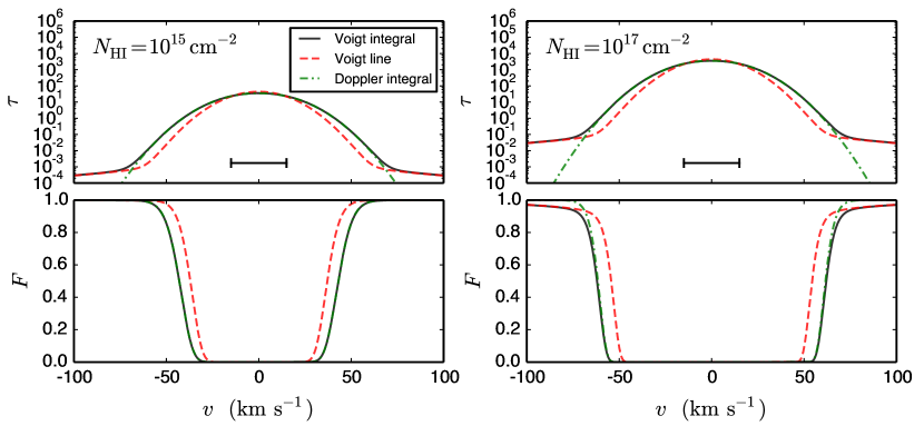
The difference in optical depth computed with a Voigt versus a Doppler profile is very small in the regime we are interested in ($\tau_{0}<100$). Figure 31 shows the optical depth to a single absorber with uniform H i density and temperature, computed three different ways. The system spans a comoving scale of roughly 300 $h^{-1}$kpc, and corresponds to $\Delta v=30$ km s^-1 for our cosmology’s $H(z=2)$. The difference between the left and right panels is the column density, where a system with a typical Ly$\alpha$ forest column density is shown on the left and a weak Lyman Limit System is on the right. The Voigt integral and Doppler integral versions are the full sightline integral, and only differ by the line profile assumed. A third computation approximates the feature as a single line with line center at the center of the absorber (“Voigt line”). The Voigt line version follows the damping wings, but has the wrong shape near line center. It does not account for the change in the line center of the gas across the system and is therefore too narrow. The Doppler integral version correctly traces the Gaussian shape near line center, but misses the damping wings. However, for the low column density lines that make up the Ly$\alpha$ forest, the damping wings add optical depth at the level of $\sim 10^{-3}$. After the transformation to $F$, such a small $\tau$ is far from detectable. For column densities of Lyman Limit Systems though, the damping wings contribute $\tau\sim 0.1$, which clearly shows up in $F$. In Ly$\alpha$ forest observations, contamination from LLSs and DLAs is masked out or taken into account in error estimates, so we actually want to avoid modeling their contamination here. Additionally, our simulations do not properly model the H i density and temperature in the high density regions that give rise to LLSs and DLAs since they do not include radiative transfer. Because the difference in the resulting optical depth is very small, and the Doppler profile is simpler and faster to compute, we use the Doppler line profile in this work.

In order to produce statistics at a single redshift, we also compute the optical depth at a fixed redshift. That is, we do not account for the speed of light when we cast rays in the simulation; we use the gas state at a single cosmic time. The simulated spectra are not meant to look like full Ly$\alpha$ forest spectra, but just recover the statistics of the flux in a small redshift window. The path length in the sightline integration is then $dr=a\,dx=dv/H$, where $r$ is the proper distance, $x$ is the comoving distance, $v$ is the Hubble flow velocity, and $H$ is the Hubble expansion rate at that redshift. In velocity coordinates, the optical depth is

$$\tau_{v}=\frac{\pi e^{2}f_{lu}\lambda_{0}}{m_{e}cH}\int n_{\rm X}\frac{1}{\pi^{1/2}b}\exp\left[-\left(\frac{v-v_{0}}{b}\right)^{2}\right]dv.$$ (25)

Although the gas data is fixed at the grid resolution, we can choose an arbitrary spectral resolution $N_{\rm pix}$ along the LOS. We also take the gas values as constant across each cell. With $i$ as the cell index, and $j$ as the pixel index, the discretized version of the optical depth is

$$\tau_{j}=\frac{\pi e^{2}f_{lu}\lambda_{0}}{m_{e}cH}\sum_{i}n_{{\rm X},i}\left[\mathrm{erf}(y_{i-1/2})-\mathrm{erf}(y_{i+1/2})\right]$$ (26)

where $y=(v_{j}-v_{\parallel,i}-v)/b$ is the line center shift from the pixel velocity in terms of the broadening scale, $v_{\parallel,i}$ is the component of the gas peculiar velocity parallel to the sightline, and $v$ is the Hubble velocity. The velocity coordinates are also periodic on the domain scale $[0,\dot{a}L)$. It is fortunate the optical depth integration reduces to an analytic expression, as this makes the calculation more robust and straightforward. Previous studies have used the midpoint expression for this integral, but we found that this created too large an error when the sampling scale $\Delta v$ was $\sim 2$ km s^-1 or larger, whereas the analytic version explicitly conserves the optical depth for any $\Delta v$.

Appendix C The Effect of Spectral Resolution

As noted in the previous section, we have the choice to evaluate the spectra at an arbitrary resolution. Given a vector of the simulated values $s_{i}=\left(n_{\rm X,i},v_{\parallel,i},b_{i}\right)$, at position $v_{i}$ along a skewer, we can evaluate the optical depth at any $v_{j}$. The resolution requirement here is essentially set by the linewidths, so that we capture all fluctuations that should be present in the spectra. Given that the most narrow lines have $b\sim 5$ km/s, the required spectral sampling should be similar.

We test that we have adequate spectral resolution by taking the L10_N512 snapshot a redshift $z=2.5$, recomputing the optical depth at lower and higher spectral resolution and checking the effect on various flux statistics. In the rest of the paper, we have taken the spectral grid to be the same as the simulation grid ($512^{3}$ in this case). Here we also try the grids 512x512x128, 256, 1024, and 2048, which spans a factor of 4 worse to 4 better than the default. We see essentially no change in the mean flux (less than $10^{-6}$). We can actually see the effect in the flux PDF, but the difference is still very small, and does not appear to be a systematic difference, but behaves more like noise from the slightly different sampling. Over all bins, the RMS difference compared to the $N_{\rm pix}=2048$ PDF is less than $10^{-3}$ in all cases. For the 1D flux power, the RMS difference is also less than $10^{-3}$ including points up to $k=30$ $h^{-1}$Mpc. On very small scales ($k>50$ $h^{-1}$Mpc), the results do depend heavily on spectral resolution, with high spectral resolution results having tens of percent larger power. However, this result is of no concern since by this scale, the dimensionless 1D power is already $<10^{-6}$. It seems that even at the worst resolution, all relevant lines are resolved.

References

- Aldrovandi & Pequignot (1973) Aldrovandi S. M. V., Pequignot D., 1973, AAP, 25, 137
- Almgren et al. (2010) Almgren A. S. et al., 2010, ApJ, 715, 1221
- Almgren et al. (2013) Almgren A. S., Bell J. B., Lijewski M. J., Lukić Z., Van Andel E., 2013, ApJ, 765, 39
- Becker et al. (2011) Becker G. D., Bolton J. S., Haehnelt M. G., Sargent W. L. W., 2011, Mon. Not. Royal Astro. Soc., 410, 1096
- Becker et al. (2013) Becker G. D., Hewett P. C., Worseck G., Prochaska J. X., 2013, Mon. Not. Royal Astro. Soc., 430, 2067
- Becker, Rauch & Sargent (2007) Becker G. D., Rauch M., Sargent W. L. W., 2007, ApJ, 662, 72
- Bi & Davidsen (1997) Bi H., Davidsen A. F., 1997, ApJ, 479, 523
- Black (1981) Black J. H., 1981, Mon. Not. Royal Astro. Soc., 197, 553
- Blas, Lesgourgues & Tram (2011) Blas D., Lesgourgues J., Tram T., 2011, J. Cosmology Astropart. Phys., 7, 34
- Bolton & Becker (2009) Bolton J. S., Becker G. D., 2009, Mon. Not. Royal Astro. Soc., 398, L26
- Bolton et al. (2014) Bolton J. S., Becker G. D., Haehnelt M. G., Viel M., 2014, Mon. Not. Royal Astro. Soc., 438, 2499
- Bolton et al. (2005) Bolton J. S., Haehnelt M. G., Viel M., Springel V., 2005, Mon. Not. Royal Astro. Soc., 357, 1178
- Borde et al. (2014) Borde A., Palanque-Delabrouille N., Rossi G., Viel M., Bolton J. S., Yèche C., LeGoff J.-M., Rich J., 2014, J. Cosmology Astropart. Phys., 7, 5
- Brown, Byrne & Hindmarsh (1989) Brown P. N., Byrne G. D., Hindmarsh A. C., 1989, SIAM J. Sci. Stat. Comput., 10, 1038
- Bryan et al. (1999) Bryan G. L., Machacek M., Anninos P., Norman M. L., 1999, ApJ, 517, 13
- Bryan & Machacek (2000) Bryan G. L., Machacek M. E., 2000, ApJ, 534, 57
- Busca et al. (2013) Busca N. G. et al., 2013, AAP, 552, A96
- Cen (1992) Cen R., 1992, ApJS, 78, 341
- Cen et al. (1994) Cen R., Miralda-Escudé J., Ostriker J. P., Rauch M., 1994, ApJL, 437, L9
- Coc, Uzan & Vangioni (2013) Coc A., Uzan J.-P., Vangioni E., 2013, ArXiv e-prints: 1307.6955
- Colella (1990) Colella P., 1990, Journal of Computational Physics, 87, 171
- Compostella, Cantalupo & Porciani (2013) Compostella M., Cantalupo S., Porciani C., 2013, Mon. Not. Royal Astro. Soc., 435, 3169
- Crighton et al. (2011) Crighton N. H. M. et al., 2011, Mon. Not. Royal Astro. Soc., 414, 28
- Croft et al. (2002) Croft R. A. C., Weinberg D. H., Bolte M., Burles S., Hernquist L., Katz N., Kirkman D., Tytler D., 2002, ApJ, 581, 20
- Croft et al. (1998) Croft R. A. C., Weinberg D. H., Katz N., Hernquist L., 1998, ApJ, 495, 44
- Croft et al. (1999) Croft R. A. C., Weinberg D. H., Pettini M., Hernquist L., Katz N., 1999, ApJ, 520, 1
- Dawson et al. (2013) Dawson K. S. et al., 2013, AJ, 145, 10
- Eisenstein & Hu (1999) Eisenstein D. J., Hu W., 1999, ApJ, 511, 5
- Faucher-Giguère, Kereš & Ma (2011) Faucher-Giguère C.-A., Kereš D., Ma C.-P., 2011, Mon. Not. Royal Astro. Soc., 417, 2982
- Faucher-Giguère et al. (2009) Faucher-Giguère C.-A., Lidz A., Zaldarriaga M., Hernquist L., 2009, ApJ, 703, 1416
- Ferland et al. (1992) Ferland G. J., Peterson B. M., Horne K., Welsh W. F., Nahar S. N., 1992, ApJ, 387, 95
- Font-Ribera et al. (2013) Font-Ribera A. et al., 2013, J. Cosmology Astropart. Phys., 5, 18
- Font-Ribera et al. (2014) Font-Ribera A. et al., 2014, J. Cosmology Astropart. Phys., 5, 27
- Font-Ribera et al. (2012) Font-Ribera A. et al., 2012, J. Cosmology Astropart. Phys., 11, 59
- Garzilli et al. (2012) Garzilli A., Bolton J. S., Kim T.-S., Leach S., Viel M., 2012, Mon. Not. Royal Astro. Soc., 424, 1723
- Gnedin & Hui (1998) Gnedin N. Y., Hui L., 1998, Mon. Not. Royal Astro. Soc., 296, 44
- Haardt & Madau (1996) Haardt F., Madau P., 1996, ApJ, 461, 20
- Haardt & Madau (2012) Haardt F., Madau P., 2012, ApJ, 746, 125
- Habib et al. (2009) Habib S. et al., 2009, Journal of Physics Conference Series, 180, 012019
- Heitmann et al. (2014) Heitmann K., Lawrence E., Kwan J., Habib S., Higdon D., 2014, ApJ, 780, 111
- Hernquist et al. (1996) Hernquist L., Katz N., Weinberg D. H., Miralda-Escudé J., 1996, ApJL, 457, L51
- Hui & Gnedin (1997) Hui L., Gnedin N. Y., 1997, Mon. Not. Royal Astro. Soc., 292, 27
- Ikeuchi (1986) Ikeuchi S., 1986, Astrophysics and Space Science, 118, 509
- Janknecht et al. (2006) Janknecht E., Reimers D., Lopez S., Tytler D., 2006, AAP, 458, 427
- Kaiser (1987) Kaiser N., 1987, Mon. Not. Royal Astro. Soc., 227, 1
- Katz, Weinberg & Hernquist (1996) Katz N., Weinberg D. H., Hernquist L., 1996, ApJS, 105, 19
- Kim et al. (2004) Kim T.-S., Viel M., Haehnelt M. G., Carswell R. F., Cristiani S., 2004, Mon. Not. Royal Astro. Soc., 347, 355
- Kollmeier et al. (2014) Kollmeier J. A. et al., 2014, ApJL, 789, L32
- Komatsu et al. (2011) Komatsu E. et al., 2011, ApJS, 192, 18
- Lee et al. (2014a) Lee K.-G., Hennawi J. F., White M., Croft R. A. C., Ozbek M., 2014a, ApJ, 788, 49
- Lee et al. (2014b) Lee K.-G. et al., 2014b, ArXiv e-prints: 1405.1072
- Lidz et al. (2010) Lidz A., Faucher-Giguère C.-A., Dall’Aglio A., McQuinn M., Fechner C., Zaldarriaga M., Hernquist L., Dutta S., 2010, ApJ, 718, 199
- McDonald (2003) McDonald P., 2003, ApJ, 585, 34
- McDonald et al. (2000) McDonald P., Miralda-Escudé J., Rauch M., Sargent W. L. W., Barlow T. A., Cen R., Ostriker J. P., 2000, ApJ, 543, 1
- McDonald et al. (2006) McDonald P. et al., 2006, ApJS, 163, 80
- McDonald et al. (2005) McDonald P. et al., 2005, ApJ, 635, 761
- McQuinn et al. (2011) McQuinn M., Hernquist L., Lidz A., Zaldarriaga M., 2011, Mon. Not. Royal Astro. Soc., 415, 977
- McQuinn et al. (2009) McQuinn M., Lidz A., Zaldarriaga M., Hernquist L., Hopkins P. F., Dutta S., Faucher-Giguère C.-A., 2009, ApJ, 694, 842
- McQuinn & White (2011) McQuinn M., White M., 2011, Mon. Not. Royal Astro. Soc., 415, 2257
- McQuinn & Worseck (2014) McQuinn M., Worseck G., 2014, Mon. Not. Royal Astro. Soc., 440, 2406
- Meiksin (2000) Meiksin A., 2000, Mon. Not. Royal Astro. Soc., 314, 566
- Meiksin, Bryan & Machacek (2001) Meiksin A., Bryan G., Machacek M., 2001, Mon. Not. Royal Astro. Soc., 327, 296
- Meiksin & Tittley (2012) Meiksin A., Tittley E. R., 2012, Mon. Not. Royal Astro. Soc., 423, 7
- Meiksin, Tittley & Brown (2010) Meiksin A., Tittley E. R., Brown C. K., 2010, Mon. Not. Royal Astro. Soc., 401, 77
- Meiksin & White (2001) Meiksin A., White M., 2001, Mon. Not. Royal Astro. Soc., 324, 141
- Meiksin & White (2004) Meiksin A., White M., 2004, Mon. Not. Royal Astro. Soc., 350, 1107
- Meiksin (2009) Meiksin A. A., 2009, Reviews of Modern Physics, 81, 1405
- Palanque-Delabrouille et al. (2013) Palanque-Delabrouille N. et al., 2013, AAP, 559, A85
- Peebles (1968) Peebles P. J. E., 1968, ApJ, 153, 1
- Petitjean, Mueket & Kates (1995) Petitjean P., Mueket J. P., Kates R. E., 1995, AAP, 295, L9
- Planck Collaboration et al. (2014) Planck Collaboration et al., 2014, AAP, 571, A16
- Rauch et al. (1997) Rauch M. et al., 1997, ApJ, 489, 7
- Rees (1986) Rees M. J., 1986, Mon. Not. Royal Astro. Soc., 218, 25P
- Ricotti, Gnedin & Shull (2000) Ricotti M., Gnedin N. Y., Shull J. M., 2000, ApJ, 534, 41
- Rudie et al. (2012) Rudie G. C. et al., 2012, ApJ, 750, 67
- Schaye et al. (2000) Schaye J., Theuns T., Rauch M., Efstathiou G., Sargent W. L. W., 2000, Mon. Not. Royal Astro. Soc., 318, 817
- Scholz & Walters (1991) Scholz T. T., Walters H. R. J., 1991, ApJ, 380, 302
- Shapiro & Kang (1987) Shapiro P. R., Kang H., 1987, ApJ, 318, 32
- Shull et al. (2010) Shull J. M., France K., Danforth C. W., Smith B., Tumlinson J., 2010, ApJ, 722, 1312
- Slosar et al. (2011) Slosar A. et al., 2011, J. Cosmology Astropart. Phys., 9, 1
- Slosar et al. (2009) Slosar A., Ho S., White M., Louis T., 2009, J. Cosmology Astropart. Phys., 10, 19
- Slosar et al. (2013) Slosar A. et al., 2013, J. Cosmology Astropart. Phys., 4, 26
- Stark et al. (2014) Stark C. W., Khandai N., Lukić Z., Nugent P., Slosar A., White M., 2014, in prep.
- Steinmetz & White (1997) Steinmetz M., White S. D. M., 1997, Mon. Not. Royal Astro. Soc., 288, 545
- Strang (1968) Strang G., 1968, SIAM J. Numerical Analysis, 5, 506
- Syphers & Shull (2014) Syphers D., Shull J. M., 2014, ApJ, 784, 42
- Theuns et al. (2002) Theuns T., Zaroubi S., Kim T.-S., Tzanavaris P., Carswell R. F., 2002, Mon. Not. Royal Astro. Soc., 332, 367
- Tittley & Meiksin (2007) Tittley E. R., Meiksin A., 2007, Mon. Not. Royal Astro. Soc., 380, 1369
- Tytler et al. (2009) Tytler D., Paschos P., Kirkman D., Norman M. L., Jena T., 2009, Mon. Not. Royal Astro. Soc., 393, 723
- Verner & Ferland (1996) Verner D. A., Ferland G. J., 1996, ApJS, 103, 467
- Viel & Haehnelt (2006) Viel M., Haehnelt M. G., 2006, Mon. Not. Royal Astro. Soc., 365, 231
- Viel, Haehnelt & Springel (2004) Viel M., Haehnelt M. G., Springel V., 2004, Mon. Not. Royal Astro. Soc., 354, 684
- Viel, Schaye & Booth (2013) Viel M., Schaye J., Booth C. M., 2013, Mon. Not. Royal Astro. Soc., 429, 1734
- Vogt et al. (1994) Vogt S. S. et al., 1994, in Presented at the Society of Photo-Optical Instrumentation Engineers (SPIE) Conference, Vol. 2198, Proc. SPIE Instrumentation in Astronomy VIII, David L. Crawford; Eric R. Craine; Eds., Volume 2198, p. 362, Crawford D. L., Craine E. R., eds., pp. 362–+
- Voronov (1997) Voronov G. S., 1997, Atomic Data and Nuclear Data Tables, 65, 1
- Worseck et al. (2014) Worseck G., Prochaska J. X., Hennawi J. F., McQuinn M., 2014, ArXiv e-prints: 1405.7405
- York et al. (2000) York D. G. et al., 2000, AJ, 120, 1579
- Zaldarriaga (2002) Zaldarriaga M., 2002, ApJ, 564, 153
- Zel’dovich (1970) Zel’dovich Y. B., 1970, AAP, 5, 84
- Zhang, Anninos & Norman (1995) Zhang Y., Anninos P., Norman M. L., 1995, ApJL, 453, L57
- Zhang et al. (1997) Zhang Y., Anninos P., Norman M. L., Meiksin A., 1997, ApJ, 485, 496
- Zhang et al. (1998) Zhang Y., Meiksin A., Anninos P., Norman M. L., 1998, ApJ, 495, 63