SPSD Matrix Approximation vis Column Selection: Theories, Algorithms, and Extensions

Abstract

Symmetric positive semidefinite (SPSD) matrix approximation is an important problem with applications in kernel methods. However, existing SPSD matrix approximation methods such as the Nyström method only have weak error bounds. In this paper we conduct in-depth studies of an SPSD matrix approximation model and establish strong relative-error bounds. We call it the prototype model for it has more efficient and effective extensions, and some of its extensions have high scalability. Though the prototype model itself is not suitable for large-scale data, it is still useful to study its properties, on which the analysis of its extensions relies.

This paper offers novel theoretical analysis, efficient algorithms, and a highly accurate extension. First, we establish a lower error bound for the prototype model and improve the error bound of an existing column selection algorithm to match the lower bound. In this way, we obtain the first optimal column selection algorithm for the prototype model. We also prove that the prototype model is exact under certain conditions. Second, we develop a simple column selection algorithm with a provable error bound. Third, we propose a so-called spectral shifting model to make the approximation more accurate when the eigenvalues of the matrix decay slowly, and the improvement is theoretically quantified. The spectral shifting method can also be applied to improve other SPSD matrix approximation models.

Keywords: Matrix approximation, matrix factorization, kernel methods, the Nyström method, spectral shifting

1 Introduction

The kernel methods are important tools in machine learning, computer vision, and data mining (Schölkopf and Smola, 2002; Shawe-Taylor and Cristianini, 2004). However, for two reasons, most kernel methods have scalability difficulties. First, given $n$ data points of $d$ dimension, generally we need ${\mathcal{O}}(n^{2}d)$ time to form the $n\times n$ kernel matrix ${\bf K}$. Second, most kernel methods require expensive matrix computations. For example, Gaussian process regression and classification require inverting some $n\times n$ matrices which costs ${\mathcal{O}}(n^{3})$ time and ${\mathcal{O}}(n^{2})$ memory; kernel PCA and spectral clustering perform the truncated eigenvalue decomposition which takes $\tilde{\mathcal{O}}(n^{2}k)$ time and ${\mathcal{O}}(n^{2})$ memory, where $k$ is the target rank of the decomposition.

Besides high time complexities, these matrix operations also have high memory cost and are difficult to implement in distributed computing facilities. The matrix decomposition and (pseudo) inverse operations are generally solved by numerical iterative algorithms, which go many passes through the matrix until convergence. Thus, the whole matrix had better been placed in main memory, otherwise in each iteration there would be a swap between memory and disk, which incurs high I/O costs and can be more expensive than CPU time. Unless the algorithm is pass-efficient, that is, it goes constant passes through the data matrix, the main memory should be at least the size of the data matrix. For two reasons, such iterative algorithms are expensive even if they are performed in distributed computing facilities such as MapReduce. First, the memory cost is too expensive for each individual machine to stand. Second, communication and synchronization must be performed in each iteration of the numerical algorithms, so the cost of each iteration is high.

Many matrix approximation methods have been proposed to make kernel machines scalable. Among them the Nyström method (Nyström, 1930; Williams and Seeger, 2001) and random features (Rahimi and Recht, 2008) are the most efficient and widely applied. However, only weak results are known (Drineas and Mahoney, 2005; Gittens and Mahoney, 2013; Lopez-Paz et al., 2014). Yang et al. (2012) showed that the Nyström method is likely a better choice than random features, both theoretically and empirically. However, even the Nyström method cannot attain high accuracy. The lower bound in (Wang and Zhang, 2013) indicates that the Nyström method costs at least $\Omega(n^{2}k/\epsilon)$ time and $\Omega(n^{1.5}k^{0.5}\epsilon^{-0.5})$ memory to attain $1+\epsilon$ Frobenius norm error bound relative to the best rank $k$ approximation.

In this paper we investigate a more accurate low-rank approximation model proposed by Halko et al. (2011); Wang and Zhang (2013), which we refer to as the prototype model. For any symmetric positive semidefinite (SPSD) matrix ${\bf K}\in{\mathbb{R}}^{n\times n}$, the prototype model first draws a random matrix ${\bf P}\in{\mathbb{R}}^{n\times c}$ and forms a sketch ${\bf C}={\bf K}{\bf P}$, and then computes the intersection matrix

$${\bf U}^{\star}\;=\;\mathop{\rm argmin}_{{\bf U}}\|{\bf K}-{\bf C}{\bf U}{\bf C}^{T}\|_{F}^{2}\;=\;{\bf C}^{\dagger}{\bf K}({\bf C}^{\dagger})^{T}\;\in\;{\mathbb{R}}^{c\times c}.$$ (1)

Finally, the model approximates ${\bf K}$ by ${\bf C}{\bf U}^{\star}{\bf C}^{T}$. With this low-rank approximation at hand, it takes time ${\mathcal{O}}(nc^{2})$ to compute the approximate matrix inversion and eigenvalue decomposition. In the following we discuss how to form ${\bf C}$ and compute ${\bf U}^{\star}$.

Column Selection vs. Random Projection. Although the sketch ${\bf C}={\bf K}{\bf P}$ can be formed by either random projection or column selection, when applied to the kernel methods, column selection is preferable to random projection. As aforementioned, suppose we are given $n$ data points of $d$ dimension. It takes time ${\mathcal{O}}(n^{2}d)$ to compute the whole of the kernel matrix ${\bf K}$, which is prohibitive when $n$ is in million scale. Unfortunately, whatever existing random projection technique is employed to form the sketch ${\bf C}$, every entry of ${\bf K}$ must be visited. In contrast, by applying data independent column selection algorithms such as uniform sampling, we can form ${\bf C}$ by observing only ${\mathcal{O}}(nc)$ entries of ${\bf K}$. At present all the existing column selection algorithms, including our proposed uniform+adaptive² algorithm, cannot avoid observing the whole of ${\bf K}$ while keeping constant-factor bound. Nevertheless, we conjecture that our uniform+adaptive² algorithm can be adapted to satisfy these two properties simultaneously (see Section 5.4 for discussions in detail).

The Intersection Matrix. With the sketch ${\bf C}$ at hand, it remains to compute the intersection matrix. The most straightforward way is (1), which minimizes the Frobenius norm approximation error. However, this approach has two drawbacks. First, it again requires the full observation of ${\bf K}$. Second, the matrix product ${\bf C}^{\dagger}{\bf K}$ costs ${\mathcal{O}}(n^{2}c)$ time. The prototype model is therefore time-inefficient. Fortunately, Wang et al. (2015) recently overcame the two drawbacks by solving (1) approximately rather than optimally. Wang et al. (2015) obtained the approximate intersection matrix $\tilde{\bf U}$ in ${\mathcal{O}}(nc^{3}/\epsilon)$ time while keeping

$$\|{\bf K}-{\bf C}\tilde{\bf U}{\bf C}^{T}\|_{F}^{2}\;\leq\;(1+\epsilon)\min_{{\bf U}}\|{\bf K}-{\bf C}{\bf U}{\bf C}^{T}\|_{F}^{2}$$ (2)

with high probability.

With the more efficient solution, why is it useful to study the exact solution to the prototype model (1)? On the one hand, from (2) we can see that the quality of the approximation depends on the prototype model, thus improvement of the prototype model directly applies to the more efficient model. On the other hand, for medium-scale problems where ${\bf K}$ does not fit in memory, the prototype model can produce high quality approximation with reasonable time expense. The experiment on kernel PCA in Section 6.3 shows that the prototype model is far more accurate than the Nyström method. For the above two reasons, we believe the study of the prototype model is useful.

1.1 Contributions

Our contributions mainly include three aspects: theoretical analysis, column selection algorithms, and extensions. They are summarized as follows.

1.1.1 Contributions: Theories

Kumar et al. (2009); Talwalkar and Rostamizadeh (2010) previously showed that the Nyström method is exact when the original kernel matrix is low-rank. In Section 4.1 we show that the prototype model exactly recovers the original SPSD matrix under the same conditions.

The prototype model with the near-optimal+adaptive column sampling algorithm satisfies $1{+}\epsilon$ relative-error bound when $c={\mathcal{O}}(k/\epsilon^{2})$ (Wang and Zhang, 2013). It was unknown whether this upper bound is optimal. In Section 4.2 we establish a lower error bound for the prototype model. We show that at least $2k/\epsilon$ columns must be chosen to attain $1+\epsilon$ bound. In Theorem 3 we improve the upper error bound of the near-optimal+adaptive algorithm to ${\mathcal{O}}(k/\epsilon)$, which matches the lower bound up to a constant factor.

1.1.2 Contributions: Algorithms

In Section 5 we devise a simple column selection algorithm which we call the uniform+adaptive² algorithm. The uniform+adaptive² algorithm is more efficiently and more easily implemented than the near-optimal+adaptive algorithm of Wang and Zhang (2013), yet its error bound is comparable with the near-optimal+adaptive algorithm. It is worth mentioning that our uniform+adaptive² algorithm is the adaptive-full algorithm of (Figure 3, Kumar et al., 2012) with two rounds of adaptive sampling, and thus our results theoretically justify the adaptive-full algorithm.

1.1.3 Contributions: Extension

When the spectrum of a matrix decays slowly (that is, the $c+1$ to $n$ largest eigenvalues are not small enough), all of the low-rank approximations are far from the original kernel matrix. Inspired by Zhang (2014), we propose a new method called spectral shifting (SS) to make the approximation still effective even when the spectrum decays slowly. Unlike the low-rank approximation ${\bf K}\approx{\bf C}{\bf U}{\bf C}^{T}$, the spectral shifting model approximates ${\bf K}$ by ${\bf K}\approx\bar{{\bf C}}{\bf U}^{\textrm{ss}}\bar{{\bf C}}^{T}+\delta^{\textrm{ss}}{\bf I}_{n}$, where ${\bf C},\bar{{\bf C}}\in{\mathbb{R}}^{n\times c}$, ${\bf U},{{\bf U}^{\textrm{ss}}}\in{\mathbb{R}}^{c\times c}$, and $\delta^{\textrm{ss}}\geq 0$. When the spectrum of ${\bf K}$ decays slowly, the term $\delta^{\textrm{ss}}{\bf I}_{n}$ helps to improve the approximation accuracy. In Section 7 we describe the spectral shifting method in detail.

We highlight that the spectral shifting method can naturally apply to improve other kernel approximation models such as the memory efficient kernel approximation (MEKA) model (Si et al., 2014). Experiments demonstrate that MEKA can be significantly improved by spectral shifting.

1.2 Paper Organization

The remainder of this paper is organized as follows. In Section 2 we define the notation. In Section 3 we introduce the motivations of SPSD matrix approximation and define the SPSD matrix approximation models. Then we present our work—theories, algorithms, and extension—respectively in Sections 4, 5, and 7. In Section 6 we conduct experiments to compare among the column sampling algorithms. In Section 8 we empirically evaluate the proposed spectral shifting model. All the proofs are deferred to the appendix.

2 Notation

Let $[n]=\{1,\ldots,n\}$, and ${\bf I}_{n}$ be the $n{\times}n$ identity matrix. For an $m{\times}n$ matrix ${\bf A}=[a_{ij}]$, we let ${\bf a}_{i:}$ be its $i$-th row, ${\bf a}_{:i}$ be its $i$-th column, and use ${\bf a}_{i}$ to denote either row or column when there is no ambiguity. Let ${\bf A}_{1}\oplus{\bf A}_{2}\oplus\cdots\oplus{\bf A}_{q}$ be the block diagonal matrix whose the $i$-th diagonal block is ${\bf A}_{i}$. Let $\|{\bf A}\|_{F}=(\sum_{i,j}a_{ij}^{2})^{1/2}$ be the Frobenius norm and $\|{\bf A}\|_{2}=\max_{{\bf x}\neq{\bf 0}}\|{\bf A}{\bf x}\|_{2}/\|{\bf x}\|_{2}$ be the spectral norm.

Letting $\rho=\mathrm{rank}({\bf A})$, we write the condensed singular value decomposition (SVD) of ${\bf A}$ as ${\bf A}={\bf U}_{\bf A}\mbox{\boldmath$\Sigma$\unboldmath}_{\bf A}{\bf V}_{\bf A}^{T}$, where the $(i,i)$-th entry of $\mbox{\boldmath$\Sigma$\unboldmath}_{\bf A}\in{\mathbb{R}}^{\rho\times\rho}$ is the $i$-th largest singular value of ${\bf A}$ (denoted $\sigma_{i}({\bf A})$). Unless otherwise specified, in this paper “SVD” means the condensed SVD. We also let ${\bf U}_{{\bf A},k}$ and ${\bf V}_{{\bf A},k}$ be the first $k$ ($<\rho$) columns of ${\bf U}_{\bf A}$ and ${\bf V}_{\bf A}$, respectively, and $\mbox{\boldmath$\Sigma$\unboldmath}_{{\bf A},k}$ be the $k\times k$ top sub-block of $\mbox{\boldmath$\Sigma$\unboldmath}_{\bf A}$. Then the $m\times n$ matrix ${\bf A}_{k}={\bf U}_{{\bf A},k}\mbox{\boldmath$\Sigma$\unboldmath}_{{\bf A},k}{\bf V}_{{\bf A},k}^{T}$ is the “closest” rank-$k$ approximation to ${\bf A}$.

If ${\bf A}$ is normal, we let ${\bf A}={\bf U}_{\bf A}\mbox{\boldmath$\Lambda$\unboldmath}_{\bf A}{\bf U}_{\bf A}^{T}$ be the eigenvalue decomposition, and denote the $i$-th diagonal entry of $\mbox{\boldmath$\Lambda$\unboldmath}_{\bf A}$ by $\lambda_{i}({\bf A})$, where $|\lambda_{1}({\bf A})|\geq\cdots\geq|\lambda_{n}({\bf A})|$. When ${\bf A}$ is SPSD, the SVD and the eigenvalue decomposition of ${\bf A}$ are identical.

Based on SVD, the matrix coherence of the columns of ${\bf A}$ relative to the best rank-$k$ approximation is defined as $\mu_{k}=\frac{n}{k}\max_{j}\big{\|}({\bf V}_{{\bf A},k})_{j:}\big{\|}_{2}^{2}$. Let ${\bf A}^{\dagger}={\bf V}_{{\bf A}}\mbox{\boldmath$\Sigma$\unboldmath}_{\bf A}^{-1}{\bf U}_{\bf A}^{T}$ be the Moore-Penrose inverse of ${\bf A}$. When ${\bf A}$ is nonsingular, the Moore-Penrose inverse is identical to the matrix inverse. Given another ${n\times c}$ matrix ${\bf C}$, we define ${\mathcal{P}}_{\bf C}({\bf A})={\bf C}{\bf C}^{\dagger}{\bf A}$ as the projection of ${\bf A}$ onto the column space of ${\bf C}$ and ${\mathcal{P}}_{{\bf C},k}({\bf A})={\bf C}\cdot\mathop{\rm argmin}_{\mathrm{rank}({\bf X})\leq k}\|{\bf A}-{\bf C}{\bf X}\|_{F}$ as the rank restricted projection. It is obvious that $\|{\bf A}-{\mathcal{P}}_{\bf C}({\bf A})\|_{F}\leq\|{\bf A}-{\mathcal{P}}_{{\bf C},k}({\bf A})\|_{F}$.

3 SPSD Matrix Approximation Models

In Section 3.1 we provide motivating examples to show why SPSD matrix approximation is useful. In Section 3.2 we formally describe low-rank approximation models. In Section 3.3 we describe the spectral shifting model. In Table 1 we compare the matrix approximation models defined in Section 3.2 and Section 3.3.

Table 1: Comparisons among the matrix approximation models in Section 3.2 and Section 3.3. Here “#Entries” denotes the number of entries of ${\bf K}$ required to observe. The costs of column selection is not counted; they are listed separately in Table 2.

	Time	Memory	#Entries	Theory
Prototype	${\mathcal{O}}(n^{2}c)$	${\mathcal{O}}(nc)$	$n^{2}$	$1+\epsilon$ relative-error
Faster	${\mathcal{O}}(nc^{3}/\epsilon)$	${\mathcal{O}}(nc)$	$nc^{2}/\epsilon$	$1+\epsilon$ relative-error
Nyström	${\mathcal{O}}(nc^{2})$	${\mathcal{O}}(nc)$	$nc$	weak
SS	the same to “prototype”			stronger than “prototype”
Faster SS	the same to “faster”			unknown

3.1 Motivations

Let ${\bf K}$ be an $n\times n$ kernel matrix. Many kernel methods require the eigenvalue decomposition of ${\bf K}$ or solving certain linear systems involving ${\bf K}$.

• Spectral clustering, kernel PCA, and manifold learning need to perform the rank $k$ eigenvalue decomposition which costs $\tilde{\mathcal{O}}(n^{2}k)$ time and ${\mathcal{O}}(n^{2})$ memory.

• Gaussian process regression and classification both require solving this kind of linear systems:

  $$({\bf K}+\alpha{\bf I}_{n}){\bf b}={\bf y},$$ (3)

  whose solution is ${\bf b}^{\star}=({\bf K}+\alpha{\bf I}_{n})^{-1}{\bf y}$. Here $\alpha$ is a constant. This costs ${\mathcal{O}}(n^{3})$ time and ${\mathcal{O}}(n^{2})$ memory.

Fortunately, if we can efficiently find an approximation in the form

$$\tilde{\bf K}\;=\;{\bf L}{\bf L}^{T}+\delta{\bf I}_{n}\;\approx\;{\bf K},$$

where $\delta\geq 0$ and ${\bf L}\in{\mathbb{R}}^{n\times l}$ with $l\ll n$, then the eigenvalue decomposition and linear systems can be approximately solved in ${\mathcal{O}}(nl^{2})$ time and ${\mathcal{O}}(nl)$ space in the following way.

• Approximate Eigenvalue Decomposition. Let ${\bf L}={\bf U}\mbox{\boldmath$\Sigma$\unboldmath}{\bf V}^{T}$ be the SVD and ${\bf U}_{\perp}$ be the orthogonal complement of ${\bf U}$. Then the full eigenvalue decomposition of $\tilde{\bf K}$ is

  $$\tilde{\bf K}\;=\;{\bf U}(\mbox{\boldmath$\Sigma$\unboldmath}^{2}+\delta{\bf I}_{l}){\bf U}^{T}+{\bf U}_{\perp}(\delta{\bf I}_{n-l}){\bf U}_{\perp}^{T}.$$

• Approximately Solving the Linear Systems. Here we use a more general form: $\tilde{\bf K}={\bf L}{\bf L}^{T}+\mbox{\boldmath$\Delta$\unboldmath}$, where $\Delta$ is a diagonal matrix with positive diagonal entries. Then

  $${\bf b}^{\star} = ({\bf K}+\alpha{\bf I}_{n})^{-1}{\bf y}\;\approx\;({\bf L}{\bf L}^{T}+\mbox{\boldmath$\Delta$\unboldmath}+\alpha{\bf I}_{n})^{-1}{\bf y}\;=\;({\bf L}{\bf L}^{T}+\mbox{\boldmath$\Delta$\unboldmath}^{\prime})^{-1}{\bf y}$$

  $$= {\mbox{\boldmath$\Delta$\unboldmath}^{\prime}}^{-1}{\bf y}-\underbrace{{\mbox{\boldmath$\Delta$\unboldmath}^{\prime}}^{-1}{\bf L}}_{n\times l}\underbrace{({\bf I}_{l}+{\bf L}^{T}{\mbox{\boldmath$\Delta$\unboldmath}^{\prime}}^{-1}{\bf L})^{-1}}_{l\times l}\underbrace{{\bf L}^{T}{\mbox{\boldmath$\Delta$\unboldmath}^{\prime}}^{-1}}_{l\times n}{\bf y}.$$

  Here the second equality is obtained by letting $\mbox{\boldmath$\Delta$\unboldmath}^{\prime}=\mbox{\boldmath$\Delta$\unboldmath}+\alpha{\bf I}_{n}$, and the third equality follows by the Sherman-Morrison-Woodbury matrix identity.

The remaining problem is to find such matrix approximation efficiently while keeping $\tilde{\bf K}$ close to ${\bf K}$.

Algorithm 1 Computing the Prototype Model in ${\mathcal{O}}(nc+nd)$ Memory.

1:  Input: data points ${\bf x}_{1},\cdots,{\bf x}_{n}\in{\mathbb{R}}^{d}$, kernel function $\kappa(\cdot,\cdot)$.

2:  Compute ${\bf C}$ and ${\bf C}^{\dagger}$; // In ${\mathcal{O}}(nc+nd)$ memory and ${\mathcal{O}}(ncd+nc^{2})$ time

3:  Form a $c\times n$ all-zero matrix ${\bf D}$; // In ${\mathcal{O}}(nc)$ memory and ${\mathcal{O}}(nc)$ time

4:  for $j=1$ to $n$  do

5:        Form the $j$-th column of ${\bf K}$ by ${\bf k}_{j}=[\kappa({\bf x}_{1},{\bf x}_{j}),\cdots,\kappa({\bf x}_{n},{\bf x}_{j})]^{T}$;

6:        Compute the $j$-th column of ${\bf D}$ by ${\bf d}_{j}={\bf C}^{\dagger}{\bf k}_{j}$;

7:        Delete ${\bf k}_{j}$ from memory;

8:  end for

9:  // Now the matrix ${\bf D}$ is ${\bf C}^{\dagger}{\bf K}$

10:  // The loop totaly costs ${\mathcal{O}}(nc+nd)$ memory and ${\mathcal{O}}(n^{2}d+n^{2}c)$ time

11:  Compute ${\bf U}={\bf D}({\bf C}^{\dagger})^{T}$; // In ${\mathcal{O}}(nc)$ memory and ${\mathcal{O}}(nc^{2})$ time

12:  return  ${\bf C}$ and ${\bf U}$ ($={\bf C}^{\dagger}{\bf K}({\bf C}^{\dagger})^{T}$).

3.2 Low-Rank Matrix Approximation Models

We first recall the prototype model introduced previously and then discuss its approximate solutions. In fact, the famous Nyström method (Nyström, 1930; Williams and Seeger, 2001) is an approximation to the prototype model. Throughout this paper, we let ${\bf P}\in{\mathbb{R}}^{n\times c}$ be random projection or column selection matrix and ${\bf C}={\bf K}{\bf P}$ be a sketch of ${\bf K}$. The only difference among the discussed models is their intersection matrices.

The Prototype Model. Suppose we have ${\bf C}\in{\mathbb{R}}^{n\times c}$ at hand. It remains to find an intersection matrix ${\bf U}\in{\mathbb{R}}^{c\times c}$. Since our objective is to make ${\bf C}{\bf U}{\bf C}^{T}$ close to ${\bf K}$, it is straightforward to optimize their difference. The prototype model computes the intersection matrix by

$${\bf U}^{\star}\;=\;\mathop{\rm argmin}_{{\bf U}}\|{\bf K}-{\bf C}{\bf U}{\bf C}^{T}\|_{F}^{2}\;=\;{\bf C}^{\dagger}{\bf K}({\bf C}^{T})^{\dagger}\;\in\;{\mathbb{R}}^{c\times c}.$$ (4)

With ${\bf C}$ at hand, the prototype model still needs one pass through the data, and it costs ${\mathcal{O}}(n^{2}c)$ time. When applied to kernel methods, the memory cost is ${\mathcal{O}}(nc+nd)$ (see Algorithm 1), where $n$ is the number of data points and $d$ is the dimension. The prototype model has the same time complexity as the exact rank $k$ eigenvalue decomposition, but it is more memory-efficient and pass-efficient.

Halko et al. (2011) showed that when ${\bf P}$ is a standard Gaussian matrix and $c={\mathcal{O}}(k/\epsilon)$, the prototype model attains $2+\epsilon$ error relative to $\|{\bf K}-{\bf K}_{k}\|_{F}^{2}$. Wang and Zhang (2013) showed that when ${\bf C}$ contains $c={\mathcal{O}}(k/\epsilon^{2})$ columns selected by the near-optimal+adaptive sampling algorithm, the prototype model attains $1+\epsilon$ relative error. In Section 5.2 we improve the result to $c={\mathcal{O}}(k/\epsilon)$, which is near optimal.

Faster SPSD matrix Approximation Model. Wang et al. (2015) noticed that (4) is a strongly over-determined linear system, and thus proposed to solve (4) by randomized approximations. They proposed to sample $s={\mathcal{O}}(c\sqrt{n/\epsilon})\ll n$ columns according to the row leverage scores of ${\bf C}$, which costs ${\mathcal{O}}(nc^{2})$ time. Let ${\bf S}\in{\mathbb{R}}^{n\times s}$ be the corresponding column selection matrix. They proposed the faster SPSD matrix approximation model which computes the intersection matrix by

$$\tilde{\bf U}\;=\;\mathop{\rm argmin}_{{\bf U}}\big{\|}{\bf S}^{T}({\bf K}-{\bf C}{\bf U}{\bf C}^{T}){\bf S}\big{\|}_{F}^{2}\;=\;\underbrace{({\bf S}^{T}{\bf C})^{\dagger}}_{c\times s}\underbrace{({\bf S}^{T}{\bf K}{\bf S})}_{s\times s}\underbrace{({\bf C}^{T}{\bf S})^{\dagger}}_{s\times c}\;\in\;{\mathbb{R}}^{c\times c}.$$ (5)

The faster model visits only $s^{2}={\mathcal{O}}(nc^{2}/\epsilon)=o(n^{2})$ entries of ${\bf K}$, and the time complexity is ${\mathcal{O}}(nc^{2}+s^{2}c)={\mathcal{O}}(nc^{3}/\epsilon)$. The following error bound is satisfied with high probability:

$$\|{\bf K}-{\bf C}\tilde{\bf U}{\bf C}^{T}\|_{F}^{2}\;\leq\;(1+\epsilon)\>\min_{{\bf U}}\|{\bf K}-{\bf C}{\bf U}{\bf C}^{T}\|_{F}^{2}.$$

This implies that if ${\bf C}$ is such a high quality sketch that the prototype model satisfies $1+\epsilon$ relative-error bound, then the faster SPSD matrix approximation model also satisfies $1+\epsilon$ relative-error bound.

The Nyström Method. The Nyström method is a special case of the faster SPSD matrix approximation model, and therefore it is also an approximate solution to (4). If we let the two column selection matrices ${\bf S}$ and ${\bf P}$ be the same, then (5) becomes

$$\tilde{\bf U}\;=\;\mathop{\rm argmin}_{{\bf U}}\big{\|}{\bf P}^{T}({\bf K}-{\bf C}{\bf U}{\bf C}^{T}){\bf P}\big{\|}_{F}^{2}\;=\;\underbrace{({\bf P}^{T}{\bf K}{\bf P})^{\dagger}}_{c\times c}\underbrace{({\bf P}^{T}{\bf K}{\bf P})}_{c\times c}\underbrace{({\bf P}^{T}{\bf K}{\bf P})^{\dagger}}_{c\times c}\;=\;\underbrace{({\bf P}^{T}{\bf K}{\bf P})^{\dagger}}_{c\times c}.$$

The matrix $({\bf P}^{T}{\bf K}{\bf P})^{\dagger}$ is exactly the intersection matrix of the Nyström method. The Nyström method costs only ${\mathcal{O}}(nc^{2})$ time, and it can be applied to million-scale problems (Talwalkar et al., 2013). However, its accuracy is low. Much work in the literature has analyzed the error bound of the Nyström method, but only weak results are known (Drineas and Mahoney, 2005; Shawe-Taylor et al., 2005; Kumar et al., 2012; Jin et al., 2013; Gittens and Mahoney, 2013). Wang and Zhang (2013) even showed that the Nyström method cannot attain $1+\epsilon$ relative-error bound unless $c\geq\Omega(\sqrt{nk/\epsilon})$. Equivalently, to attain $1+\epsilon$ bound, the Nyström would take $\Omega(n^{2}k/\epsilon)$ time and $\Omega(n^{1.5}k^{0.5}\epsilon^{-0.5})$ memory.

3.3 Spectral Shifting Models

We propose a more accurate SPSD matrix approximation method called the spectral shifting model. Here we briefly describe the model and its fast solution. The theoretical analysis is left to Section 7.

The Spectral Shifting (SS) Model. As before, we let ${\bf P}\in{\mathbb{R}}^{n\times c}$ be a column selection matrix and $\bar{\bf C}=\bar{\bf K}{\bf P}$, where $\bar{\bf K}={\bf K}$ or $\bar{\bf K}={\bf K}-\bar{\delta}{\bf I}_{n}$ for some parameter $\bar{\delta}\geq 0$. We approximate ${\bf K}$ by $\bar{\bf C}{\bf U}^{\textrm{ss}}\bar{\bf C}^{T}+\delta^{\textrm{ss}}{\bf I}_{n}$, where

$$\big{(}{\bf U}^{\textrm{ss}},\delta^{\textrm{ss}}\big{)}\;=\;\mathop{\rm argmin}_{{\bf U},\delta}\big{\|}{\bf K}-\bar{{\bf C}}{\bf U}\bar{{\bf C}}^{T}-\delta{\bf I}_{n}\big{\|}_{F}^{2}.$$ (6)

This optimization problem has closed-form solution (see Theorem 6)

$$\delta^{\textrm{ss}} = \frac{1}{n-\mathrm{rank}(\bar{{\bf C}})}\Big{(}\mathrm{tr}({\bf K})-\mathrm{tr}\big{(}{\bar{{\bf C}}}^{\dagger}{\bf K}{\bar{{\bf C}}}\big{)}\Big{)},$$

$${\bf U}^{\textrm{ss}} = {\bar{{\bf C}}}^{\dagger}{\bf K}({\bar{{\bf C}}}^{\dagger})^{T}-\delta^{\textrm{ss}}({\bar{{\bf C}}}^{T}{\bar{{\bf C}}})^{{\dagger}},$$

which can be computed in ${\mathcal{O}}(n^{2}c)$ time and ${\mathcal{O}}(nc)$ memory. Later we will show that the SS model is more accurate than the prototype model.

Faster Spectral Shifting Model. The same idea of Wang et al. (2015) also applies to the SS model (14). Specifically, we can draw another column selection matrix ${\bf S}\in{\mathbb{R}}^{n\times s}$ and solve

$$\big{(}\tilde{\bf U}^{\textrm{ss}},\tilde{\delta}^{\textrm{ss}}\big{)} = \mathop{\rm argmin}_{{\bf U},\delta}\big{\|}{\bf S}^{T}\big{(}{\bf K}-\bar{{\bf C}}{\bf U}\bar{{\bf C}}^{T}-\delta{\bf I}_{n}\big{)}{\bf S}\big{\|}_{F}^{2}$$

$$= \mathop{\rm argmin}_{{\bf U},\delta}\big{\|}{\bf S}^{T}{\bf K}{\bf S}-({\bf S}^{T}\bar{{\bf C}}){\bf U}({\bf S}^{T}\bar{{\bf C}})^{T}-\delta{\bf I}_{s}\big{\|}_{F}^{2}.$$

Similarly, it has closed-form solution

$$\tilde{\delta}^{\textrm{ss}} = \frac{1}{s-\mathrm{rank}({\bf S}^{T}\bar{{\bf C}})}\Big{[}\mathrm{tr}\big{(}{\bf S}^{T}{\bf K}{\bf S}\big{)}-\mathrm{tr}\Big{(}({\bf S}^{T}\bar{{\bf C}})^{\dagger}({\bf S}^{T}{\bf K}{\bf S})({\bf S}^{T}\bar{{\bf C}})\Big{)}\Big{]},$$

$$\tilde{\bf U}^{\textrm{ss}} = ({\bf S}^{T}\bar{{\bf C}})^{\dagger}({\bf S}^{T}{\bf K}{\bf S})({\bar{{\bf C}}}^{T}{\bf S})^{\dagger}-\tilde{\delta}^{\textrm{ss}}({\bar{{\bf C}}}^{T}{\bf S}{\bf S}^{T}{\bar{{\bf C}}})^{{\dagger}}.$$

In this way, the time cost is merely ${\mathcal{O}}(s^{2}c)$. However, the theoretical properties of this model are yet unknown. We do not conduct theoretical or empirical study of this model; we leave it as a future work,

4 Theories

In Section 4.1 we show that the prototype model is exact when ${\bf K}$ is low-rank. In Section 4.2 we provide a lower error bound of the prototype model.

4.1 Theoretical Justifications

Let ${\bf P}$ be a column selection matrix, ${\bf C}={\bf K}{\bf P}$ be a sketch, and ${\bf W}={\bf P}^{T}{\bf K}{\bf P}$ be the corresponding submatrix. Kumar et al. (2009); Talwalkar and Rostamizadeh (2010) showed that the Nyström method is exact when $\mathrm{rank}({\bf W})=\mathrm{rank}({\bf K})$. We present a similar result in Theorem 1.

Theorem 1

The following three statements are equivalent: (i) $\mathrm{rank}({\bf W})=\mathrm{rank}({\bf K})$, (ii) ${\bf K}={\bf C}{\bf W}^{\dagger}{\bf C}^{T}$, (iii) ${\bf K}={\bf C}{\bf C}^{\dagger}{\bf K}({\bf C}^{\dagger})^{T}{\bf C}^{T}$.

Theorem 1 implies that the prototype model and the Nyström method are equivalent when $\mathrm{rank}({\bf W})=\mathrm{rank}({\bf K})$; that is, the kernel matrix ${\bf K}$ is low rank. However, it holds in general that $\mathrm{rank}({\bf K})\gg c\geq\mathrm{rank}({\bf W})$, where the two models are not equivalent.

4.2 Lower Bound

Wang and Zhang (2013) showed that with $c={\mathcal{O}}(k/\epsilon^{2})$ columns chosen by the near-optimal+adaptive sampling algorithm, the prototype model satisfies $1+\epsilon$ relative-error bound. We establish a lower error bound in Theorem 2, which shows that at least $c\geq 2k\epsilon^{-1}$ columns must be chosen to attain the $1+\epsilon$ bound. This indicates there exists a gap between the upper bound in (Wang and Zhang, 2013) and our lower bound, and thus there is room of improvement. The proof of Theorem 2 is left to Appendix B.

Theorem 2 (Lower Bound of the Prototype Model)

Whatever column sampling algorithm is used, there exists an $n\times n$ SPSD matrix ${\bf K}$ such that the error incurred by the prototype model obeys:

$$\big{\|}{\bf K}-{\bf C}{\bf U}^{\star}{\bf C}^{T}\big{\|}_{F}^{2} \geq \frac{n-c}{n-k}\Big{(}1+\frac{2k}{c}\Big{)}\|{\bf K}-{\bf K}_{k}\|_{F}^{2}.$$

Here $k$ is an arbitrary target rank, $c$ is the number of selected columns, and ${\bf U}^{\star}={\bf C}^{\dagger}{\bf K}({\bf C}^{\dagger})^{T}$.

5 Column Sampling Algorithms

In Section 5.1 we introduce the column sampling algorithms in the literature. In Section 5.2 we improve the bound of the near-optimal+adaptive sampling algorithm (Wang and Zhang, 2013), and the obtained upper bound matches the lower bound up to a constant factor. In Section 5.3 we develop a more efficient column sampling algorithm which we call the uniform+adaptive² algorithm. In Section 5.4 we discuss the possibility of making uniform+adaptive² more scalable.

5.1 Related Work

Column selection is an important matrix sketching approach that enables expensive matrix computations to be performed on much a smaller matrix. The column selection problem has been widely studied in the theoretical computer science community (Boutsidis et al., 2014; Mahoney, 2011; Guruswami and Sinop, 2012; Woodruff, 2014) and the numerical linear algebra community (Gu and Eisenstat, 1996; Stewart, 1999), and numerous algorithms have been devised and analyzed. Here we focus on some provable algorithms studied in the theoretical computer science community.

The adaptive sampling algorithm devised by Deshpande et al. (2006) (see Algorithm 2) is the most relevant to this paper. The adaptive sampling algorithm has strong error bound (Deshpande et al., 2006; Wang and Zhang, 2013; Boutsidis et al., 2014) and good empirical performance (Kumar et al., 2012). Particularly, Wang and Zhang (2013) proposed an algorithm that combines the near-optimal column sampling algorithm (Boutsidis et al., 2014) and the adaptive sampling algorithm (Deshpande et al., 2006). They showed that by selecting $c={\mathcal{O}}(k\epsilon^{-2})$ columns of ${\bf K}$ to form ${\bf C}$, it holds that

$${\mathbb{E}}\big{\|}{\bf K}-{\bf C}\big{(}{\bf C}^{\dagger}{\bf K}({\bf C}^{\dagger})^{T}\big{)}{\bf C}^{T}\big{\|}_{F}\;\leq\;(1+\epsilon)\|{\bf K}-{\bf K}_{k}\|_{F}.$$

This error bound was the tightest among all the feasible algorithms for SPSD matrix approximation.

Algorithm 2 The Adaptive Sampling Algorithm.

1:  Input: a residual matrix ${\bf B}\in{\mathbb{R}}^{n\times n}$ and number of selected columns $c$ $(<n)$.

2:  Compute sampling probabilities $p_{j}=\|{\bf b}_{:j}\|_{2}^{2}/\|{\bf B}\|_{F}^{2}$ for $j=1,\cdots,n$;

3:  Select $c$ indices in $c$ i.i.d. trials, in each trial the index $j$ is chosen with probability $p_{j}$;

4:  return  an index set containing the indices of the selected columns.

5.2 Near Optimal Column Selection for SPSD Matrix Approximation

The error bound of near-optimal+adaptive can be improved by a factor of $\epsilon$ by exploiting the latest results of Boutsidis and Woodruff (2014). Using the same algorithm except for different $c_{2}$ (i.e. the number of columns selected by adaptive sampling), we obtain the following stronger theorem. Recall from Theorem 2 that the lower bound is $c\geq\Omega\big{(}2k\epsilon^{-1}(1+o(1))\big{)}$. Thus the near-optimal+adaptive algorithm is optimal up to a constant factor. The proof of the theorem is left to Appendix 3.

Theorem 3 (Near-Optimal+Adaptive)

Given a symmetric matrix ${\bf K}\in{\mathbb{R}}^{n\times n}$ and a target rank $k$, the algorithm samples totally $c=3k\epsilon^{-1}\big{(}1+o(1)\big{)}$ columns of ${\bf K}$ to construct the approximation. Then

$${\mathbb{E}}\big{\|}{\bf K}-{\bf C}\big{(}{\bf C}^{\dagger}{\bf K}({\bf C}^{\dagger})^{T}\big{)}{\bf C}^{T}\big{\|}_{F}\;\leq\;(1+\epsilon)\|{\bf K}-{\bf K}_{k}\|_{F}.$$

The algorithm costs ${\mathcal{O}}\big{(}n^{2}c+nk^{3}\epsilon^{-2/3}\big{)}$ time and ${\mathcal{O}}(nc)$ memory in computing ${\bf C}$.

Despite its optimal error bound, the near-optimal+adaptive algorithm lacks of practicality. The implementation is complicated and difficult. Its main component—the near-optimal algorithm (Boutsidis et al., 2014)—is highly iterative and therefore not suitable for parallel computing. Every step of the near-optimal algorithm requires the full observation of ${\bf K}$ and there is no hope to avoid this. Thus we propose to use uniform sampling to replace the near-optimal algorithm. Although the obtained uniform+adaptive² algorithm also has quadratic time complexity and requires the full observation of ${\bf K}$, there may be some way to making it more efficient. See the discussions in Section 5.4.

Algorithm 3 The Uniform+Adaptive² Algorithm.

1:  Input: an $n\times n$ symmetric matrix ${\bf K}$, target rank $k$, error parameter $\epsilon\in(0,1]$, matrix coherence $\mu$.

2:  Uniform Sampling. Uniformly sample

$$c_{1}=20\mu k\log\big{(}20k\big{)}\vspace{-1mm}$$

columns of ${\bf K}$ without replacement to construct ${\bf C}_{1}$;

3:  Adaptive Sampling. Sample

$$c_{2}=17.5k/\epsilon\vspace{-1mm}$$

columns of ${\bf K}$ to construct ${\bf C}_{2}$ using the adaptive sampling algorithm (Algorithm 2) according to the residual ${\bf K}-{\mathcal{P}}_{{\bf C}_{1}}({\bf K})$;

4:  Adaptive Sampling. Sample

$$c_{3}=10k/\epsilon\vspace{-1mm}$$

columns of ${\bf K}$ to construct ${\bf C}_{3}$ using the adaptive sampling algorithm (Algorithm 2) according to the residual ${\bf K}-{\mathcal{P}}_{[{\bf C}_{1},\;{\bf C}_{2}]}({\bf K})$;

5:  return  ${\bf C}=[{\bf C}_{1},{\bf C}_{2},{\bf C}_{3}]$.

5.3 The Uniform+Adaptive² Column Sampling Algorithm

In this paper we propose a column sampling algorithm which is efficient, effective, and very easy to be implemented. The algorithm consists of a uniform sampling step and two adaptive sampling steps, so we call it the uniform+adaptive² algorithm. The algorithm is described in Algorithm 3 and analyzed in Theorem 4. The proof is left to Appendix D.

It is worth mentioning that our uniform+adaptive² algorithm is a special instance of the adaptive-full algorithm of (Kumar et al., 2012, Figure 3). The adaptive-full algorithm consists of random initialization and multiple adaptive sampling steps. Using multiple adaptive sampling steps can surely reduce the approximation error. However, the update of sampling probability in each step is expensive, so we choose to do only two steps. The adaptive-full algorithm of (Kumar et al., 2012, Figure 3) is merely a heuristic scheme without theoretical guarantee; our result provides theoretical justification for the adaptive-full algorithm.

Theorem 4 (Uniform+Adaptive²)

Given an $n{\times}n$ symmetric matrix ${\bf K}$ and a target rank $k$, let $\mu_{k}$ denote the matrix coherence of ${\bf K}$. Algorithm 3 samples totally

$$c={\mathcal{O}}\big{(}k\epsilon^{-1}+\mu_{k}k\log k\big{)}$$

columns of ${\bf K}$ to construct the approximation. The error bound

$$\big{\|}{\bf K}-{\bf C}\big{(}{\bf C}^{\dagger}{\bf K}({\bf C}^{{\dagger}})^{T}\big{)}{\bf C}^{T}\big{\|}_{F}\;\leq\;\big{(}1+\epsilon\big{)}\big{\|}{\bf K}-{\bf K}_{k}\big{\|}_{F}$$

holds with probability at least $0.7$. The algorithm costs ${\mathcal{O}}(n^{2}c)$ time and ${\mathcal{O}}(nc)$ space in computing ${\bf C}$.

Remark 5

Theoretically, Algorithm 3 requires computing the matrix coherence of ${\bf K}$ in order to determine $c_{1}$ and $c_{2}$. However, computing the matrix coherence is as hard as computing the truncated SVD; even the fast approximation approach of Drineas et al. (2012) is not feasible here because ${\bf K}$ is a square matrix. The use of the matrix coherence here is merely for theoretical analysis; setting the parameter $\mu$ in Algorithm 3 to be exactly the matrix coherence does not certainly result in the highest accuracy. Empirically, the resulting approximation accuracy is not sensitive to the value of $\mu$. Thus we suggest setting $\mu$ in Algorithm 3 as a constant (e.g. $1$), rather than actually computing the matrix coherence.

Table 2: Comparisons between the two sampling algorithms.

	Uniform+Adaptive2	Near-Optimal+Adaptive
Time	${\mathcal{O}}(n^{2}c)$	${\mathcal{O}}(n^{2}c+nk^{3}\epsilon^{-2/3})$
Memory	${\mathcal{O}}\big{(}nc\big{)}$	${\mathcal{O}}\big{(}nc\big{)}$
#Passes	$2$	$4$
#Columns	${\mathcal{O}}\big{(}k\epsilon^{-1}+\mu_{k}k\log k\big{)}$	${\mathcal{O}}\big{(}k\epsilon^{-1})$
Implement	Easy to implement	Hard to implement

Table 2 presents comparisons between the near-optimal+adaptive algorithm and our uniform+adaptive² algorithm over the time cost, memory cost, number of passes through ${\bf K}$, the number of columns required to attain $1+\epsilon$ relative-error bound, and the hardness of implementation. Our algorithm is more time-efficient and pass-efficient than the near-optimal+adaptive algorithm, and the memory costs of the two algorithms are the same. To attain the same error bound, our algorithm needs to select $c={\mathcal{O}}\big{(}k\epsilon^{-1}+\mu_{k}k\log k\big{)}$ columns, which is a little larger than that of the near-optimal+adaptive algorithm.

5.4 Discussions

The two algorithms discussed in the above have strong theoretical guarantees, but they are not efficient enough for large-scale applications. First, their time complexities are quadratic in $n$. Second, they require the full observation of ${\bf K}$. In fact, at present no existing column selection algorithm satisfies the three properties simultaneously:

1. the time and memory costs are ${\mathcal{O}}(n)$;

2. only ${\mathcal{O}}(n)$ entries of ${\bf K}$ need to be observed;

3. relative-error bound holds in expectation or with high probability.

It is interesting to find such an algorithm, and it remains an open problem.

Nevertheless, uniform+adaptive² is a promising column selection algorithm for it may be adapted to satisfy the above three properties. The drawback of uniform+adaptive² is that computing the adaptive sampling probability costs quadratic time and requires the full observation of ${\bf K}$. There may be remedies for this problem. The adaptive-partial algorithm in (Kumar et al., 2012) satisfies the first two properties, but it lacks theoretical analysis. Another possibility is to first uniformly sample $o(n)$ columns and then down-sample to ${\mathcal{O}}(k/\epsilon)$ columns by adaptive sampling, which we describe in Algorithm 4. In this way, the first two properties can be satisfied, and it may be theoretically explained under the incoherent matrix assumption. We do not implement such heuristics for their theoretical property is completely unknown and they are beyond the scope of this paper.

Algorithm 4 The Incomplete Uniform+Adaptive² Algorithm.

1:  Input: part of an $n\times n$ symmetric matrix ${\bf K}$.

2:  Uniform Sampling. Uniformly sample $c_{1}$ columns of ${\bf K}$ without replacement to construct ${\bf C}_{1}$;

3:  Adaptive Sampling. Uniformly sample $o(n)$ columns of ${\bf K}$ to form ${\bf K}^{\prime}$; then sample $c_{2}$ columns of ${\bf K}^{\prime}$ to construct ${\bf C}_{2}$ using the adaptive sampling algorithm (Algorithm 2) according to the residual ${\bf K}^{\prime}-{\mathcal{P}}_{{\bf C}_{1}}({\bf K}^{\prime})$;

4:  Adaptive Sampling. Uniformly sample $o(n)$ columns of ${\bf K}$ to form ${\bf K}^{\prime\prime}$; then sample $c_{3}$ columns of ${\bf K}^{\prime\prime}$ to construct ${\bf C}_{3}$ using the adaptive sampling algorithm (Algorithm 2) according to the residual ${\bf K}^{\prime\prime}-{\mathcal{P}}_{[{\bf C}_{1},\;{\bf C}_{2}]}({\bf K}^{\prime\prime})$;

5:  return  ${\bf C}=[{\bf C}_{1},{\bf C}_{2},{\bf C}_{3}]$.

Table 3: A summary of the datasets for kernel approximation.

Dataset	MNIST	Letters	PenDigit	Cpusmall	Mushrooms
#Instance	$60,000$	$15,000$	10,992	$8,192$	$8,124$
#Attribute	$780$	$16$	16	$12$	$112$
$\gamma$ ($\eta=0.5$)	$\approx 1.50$	$0.155$	$0.045$	$0.031$	$0.850$
$\gamma$ ($\eta=0.9$)	$\approx 2.30$	$0.290$	$0.073$	$0.057$	$1.140$

Figure 1: The ratio $\frac{c}{n}$ against the error ratio defined in (8). In each subfigure, the left corresponds to the RBF kernel matrix with $\eta=0.5$, and the right corresponds to $\eta=0.9$, where $\eta$ is defined in (7).

Figure 2: The growth of the average elapsed time in $\frac{c}{n}$.

6 Experiments on the Column Sampling Algorithms

We empirically conduct comparison among three column selection algorithms—uniform sampling, uniform + adaptive², and the near-optimal + adaptive sampling algorithm.

6.1 Experiment Setting

We perform experiments on several datasets collected on the LIBSVM website where the data are scaled to [0,1]. We summarize the datasets in Table 3.

For each dataset, we generate a radial basis function (RBF) kernel matrix ${\bf K}$ defined by $k_{ij}=\exp(-\frac{1}{2\gamma^{2}}\|{\bf x}_{i}-{\bf x}_{j}\|_{2}^{2})$. Here $\gamma>0$ is the scaling parameter; the larger the scaling parameter $\gamma$ is, the faster the spectrum of the kernel matrix decays (Gittens and Mahoney, 2013). The previous work has shown that for the same dataset, with different settings of $\gamma$, the sampling algorithms have very different performances. Instead of setting $\gamma$ arbitrarily, we set $\gamma$ in the following way.

Letting $p=\lceil 0.05n\rceil$, we define

$$\eta\;\triangleq\;\frac{\sum_{i=1}^{p}\lambda_{i}^{2}({\bf K})}{\sum_{i=1}^{n}\lambda_{i}^{2}({\bf K})}\;=\;\frac{\|{\bf K}_{p}\|_{F}^{2}}{\|{\bf K}\|_{F}^{2}},$$ (7)

which denotes the ratio of the top $5\%$ eigenvalues of the kernel matrix ${\bf K}$ to the all eigenvalues. In general, a large $\gamma$ results in a large $\eta$. For each dataset, we use two different settings of $\gamma$ such that $\eta=0.5$ or $\eta=0.9$.

The models and algorithms are all implemented in MATLAB. We run the algorithms on a workstation with Intel Xeon 2.40GHz CPUs, 24GB memory, and 64bit Windows Server 2008 system. To compare the running time, we set MATLAB in single thread mode by the command “$\mathrm{maxNumCompThreads(1)}$”. In the experiments we do not keep ${\bf K}$ in memory. We use a variant of Algorithm 1—we compute and store one block, instead of one column, of ${\bf K}$ at a time. We keep at most $1,000$ columns of ${\bf K}$ in memory at a time.

We set the target rank $k$ to be $k=\lceil n/100\rceil$ in all the experiments unless otherwise specified. We evaluate the performance by

$$\textrm{Approximation Error}\;=\;{\|{\bf K}-\tilde{{\bf K}}\|_{F}}/{\|{\bf K}\|_{F}},$$ (8)

where $\tilde{{\bf K}}$ is the approximation generated by each method.

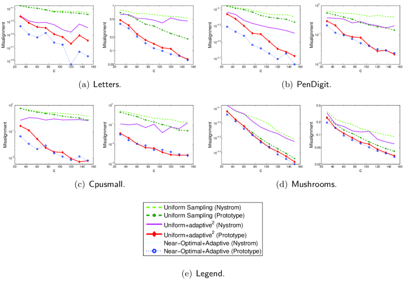
To evaluate the quality of the approximate rank-$k$ eigenvalue decomposition, we use misalignment to indicate the distance between the true eigenvectors ${\bf U}_{k}$ ($n\times k$) and the approximate eigenvectors $\tilde{\bf V}_{k}$ ($n\times k$):

$$\textrm{Misalignment}\;=\;\frac{1}{k}\big{\|}{\bf U}_{k}-\tilde{\bf V}_{k}\tilde{\bf V}_{k}^{T}{\bf U}_{k}\big{\|}_{F}^{2}\;\in\;[0,1].$$ (9)

Figure 3: The number of selected columns $c$ against the misalignment (log-scale) defined in (9). In each subfigure, the left corresponds to the RBF kernel matrix with $\eta=0.5$, and the right corresponds to $\eta=0.9$, where $\eta$ is defined in (7).

Figure 4: The elapsed time (log-scale) against the misalignment (log-scale) defined in (9). In each subfigure, the left corresponds to the RBF kernel matrix with $\eta=0.5$, and the right corresponds to $\eta=0.9$, where $\eta$ is defined in (7).

6.2 Matrix Approximation Accuracy

In the first set of experiments, we compare the matrix approximation quality using the Frobenius norm approximation error defined in (8) as the metric.

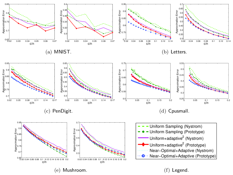
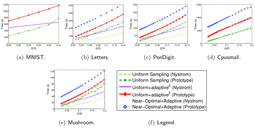
Every time when we do column sampling, we repeat each sampling algorithm $10$ times and record the minimal approximation error of the $10$ repeats. We report the average elapsed time of the $10$ repeat rather than the total elapsed time because the $10$ repeats can be done in parallel on $10$ machines. We plot $c$ against the approximation error in Figure 1. For the kernel matrices with $\eta=0.9$, we plot $c$ against the average elapsed time in Figure 2; for $\eta=0.5$, the curve of the running time is very similar, so we do not show it.

The results show that our uniform+adaptive² algorithm achieves accuracy comparable with the near-optimal+adaptive algorithm. Especially, when $c$ is large, these two algorithms have virtually the same accuracy, which agrees with our analysis: a large $c$ implies a small error term $\epsilon$, and the error bounds of the two algorithms coincide when $\epsilon$ is small. As for the running time, we can see that our uniform+adaptive² algorithm is much more efficient than the near-optimal+adaptive algorithm.

Particularly, the MNIST dataset has $60,000$ instances, and the $60,000\times 60,000$ kernel matrix ${\bf K}$ does not fit in memory. The experiment shows that neither the prototype model nor the uniform+adaptive² algorithm require keeping ${\bf K}$ in memory.

6.3 Kernel Principal Component Analysis

In the second set of experiment, we apply the kernel approximation methods to approximately compute the rank $k=3$ eigenvalue decomposition of the RBF kernel matrix. We use the misalignment defined in (9) as the metric, which reflects the distance between the true and the approximate eigenvectors. We report the average misalignment of the 20 repeats. We do not conduct experiments on the MNIST dataset because the true eigenvectors are too expensive to compute.

To evaluate the memory efficiency, we plot $c$ against the misalignment in Figure 3. The results show that the two non-uniform sampling algorithms are significantly better than uniform sampling. The performance of our uniform+adaptive² algorithm is nearly the same to the near-optimal+adaptive algorithm.

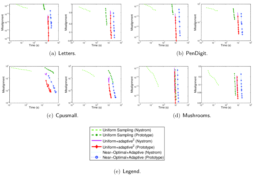
To evaluate the time efficiency, we plot the elapsed time against the misalignment in Figure 4. Though the uniform sampling algorithm is the most efficient in most cases, its accuracy is unsatisfactory. In terms of time efficiency, the uniform+adaptive² algorithm is better than the near-optimal+adaptive algorithm.

The experiment on the kernel PCA shows that the prototype model with the uniform + adaptive² column sampling algorithm achieves the best performance. Though the Nyström method with uniform sampling is the most efficient, its resulting misalignment is worse by an order of magnitude. Therefore, when applied to speedup eigenvalue decomposition, the Nyström method may not be a good choice, especially when high accuracy is required.

6.4 Separating the Time Costs

Besides the total elapsed time, the readers may be interested in the time cost of each step, especially when the data do no fit in memory. We run the Nyström method and the prototype model, each with uniform+adaptive² column sampling algorithm, on the MNIST dataset with $\gamma=2.3$ (see Table 3). Notice that the $60,000\times 60,000$ kernel matrix does not fit in memory, so we keep at most $1,000$ columns of the kernel matrix in memory at a time. We set $c=50$ or $500$ and repeat the procedure $20$ times and record the average elapsed time. In Figure 5 we separately show the time costs of the uniform+adaptive² algorithm and the computation of the intersection matrices. In addition, we separate the time costs of evaluating the kernel functions and all the other computations (e.g.  SVD of ${\bf C}$ and matrix multiplications).

(a) $c=50$

(b) $c=500$

Figure 5: The time costs (s) of the uniform+adaptive² algorithm and the computation of the intersection matrices.

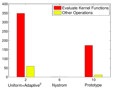
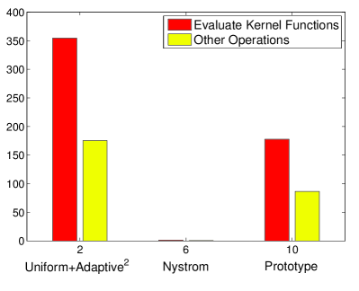
We can see from Figure 5 that when ${\bf K}$ does not fit in memory, the computation of the kernel matrix contributes to the most of the computations. By comparing the two subfigures in Figure 5, we can see that as $c$ increases, the costs of computing the kernel matrix barely change, but the costs of other matrix operations significantly increase.

7 The Spectral Shifting Model

All the low-rank approximation methods work well only when the bottom eigenvalues of ${\bf K}$ are near zero. In this section we develop extensions of the three SPSD matrix approximation models to tackle matrices with relatively big bottom eigenvalues. We call the proposed method the spectral shifting (SS) model and describe it in Algorithm 5. We show that the SS model has stronger error bound than the prototype model.

In Section 7.1 we formulate the SS model. In Section 7.2 we study SS from an optimization perspective. In Section 7.3 we show that SS has better error bound than the prototype model. Especially, with the near-optimal+adaptive column sampling algorithm, SS demonstrates much stronger error bound than the existing matrix approximation methods. In Section 7.4 we provide an efficient algorithm for computing the initial spectral shifting term. In Section 7.5 we discuss how to combine spectral shifting with other kernel approximation methods.

Algorithm 5 The Spectral Shifting Method.

1:  Input: an $n\times n$ SPSD matrix ${\bf K}$, a target rank $k$, the number of sampled columns $c$, the oversampling parameter $l$.

2:  // (optional) approximately do the initial spectral shifting

3:  $\mbox{\boldmath$\Omega$\unboldmath}\longleftarrow n\times l$ standard Gaussian matrix;

4:  ${\bf Q}\longleftarrow$ the $l$ orthonormal basis of ${\bf K}\mbox{\boldmath$\Omega$\unboldmath}\in{\mathbb{R}}^{n\times l}$;

5:  $s\longleftarrow$ sum of the top $k$ singular values of ${\bf Q}^{T}{\bf K}\in{\mathbb{R}}^{l\times n}$;

6:  $\tilde{\delta}=\frac{1}{n-k}\big{(}\mathrm{tr}({\bf K})-s\big{)}\approx\bar{\delta}$;

7:  $\bar{{\bf K}}\leftarrow{\bf K}-\tilde{\delta}{\bf I}_{n}\in{\mathbb{R}}^{n\times n}$;

8:  // perform sketching, e.g. random projection or column selection

9:  $\bar{{\bf C}}=\bar{\bf K}{\bf P}$, where ${\bf P}$ is an $n\times c$ random projection or selection matrix;

10:  Optional: replace $\bar{\bf C}$ by its orthonormal bases;

11:  // compute the spectral shifting parameter and the intersection matrix

12:  $\delta^{\textrm{ss}}\longleftarrow\frac{1}{n-\mathrm{rank}(\bar{{\bf C}})}\Big{(}\mathrm{tr}({\bf K})-\mathrm{tr}\big{(}\bar{{\bf C}}^{\dagger}{\bf K}\bar{{\bf C}}\big{)}\Big{)}$;

13:  ${\bf U}^{\textrm{ss}}\longleftarrow\bar{{\bf C}}^{\dagger}{\bf K}(\bar{{\bf C}}^{\dagger})^{T}-\delta^{\textrm{ss}}(\bar{{\bf C}}^{T}\bar{{\bf C}})^{{\dagger}}$;

14:  return  the approximation $\tilde{{\bf K}}_{c}^{\textrm{ss}}=\bar{{\bf C}}{\bf U}^{\textrm{ss}}\bar{{\bf C}}^{T}+\delta^{\textrm{ss}}{\bf I}_{n}$.

7.1 Model Formulation

The spectral shifting (SS) model is defined by

$${\tilde{{\bf K}}_{c}^{\textrm{ss}}}\;=\;\bar{{\bf C}}{\bf U}^{\textrm{ss}}\bar{{\bf C}}^{T}+\delta^{\textrm{ss}}{\bf I}_{n}.$$ (10)

Here $\delta^{\textrm{ss}}\geq 0$ is called the spectral shifting term. This approximation is computed in three steps. Firstly, (approximately) compute the initial spectral shifting term

$$\bar{\delta}\;=\;\frac{1}{n-k}\bigg{(}\mathrm{tr}({\bf K})-\sum_{j=1}^{k}\sigma_{j}({\bf K})\bigg{)},$$ (11)

and then perform spectral shifting $\bar{{\bf K}}={\bf K}-\bar{\delta}{\bf I}_{n}$, where $k\leq c$ is the target rank. This step is optional. Due to Theorem 6 and Remark 7, SS is better than the prototype model even if $\bar{\delta}=0$; however, without this step, the quantity of the improvement contributed by SS is unknown. Secondly, draw a column selection matrix ${\bf P}$ and form the sketch $\bar{\bf C}=\bar{\bf K}{\bf P}$. Finally, with $\bar{{\bf C}}$ at hand, compute $\delta^{\textrm{ss}}$ and ${\bf U}^{\textrm{ss}}$ by

$$\delta^{\textrm{ss}} = \frac{1}{n-\mathrm{rank}(\bar{{\bf C}})}\Big{(}\mathrm{tr}({\bf K})-\mathrm{tr}\big{(}{\bar{{\bf C}}}^{\dagger}{\bf K}{\bar{{\bf C}}}\big{)}\Big{)},$$

$${\bf U}^{\textrm{ss}} = {\bar{{\bf C}}}^{\dagger}{\bf K}({\bar{{\bf C}}}^{\dagger})^{T}-\delta^{\textrm{ss}}({\bar{{\bf C}}}^{T}{\bar{{\bf C}}})^{{\dagger}}.$$ (12)

We will show that ${\tilde{{\bf K}}_{c}^{\textrm{ss}}}$ is positive (semi)definite if ${\bf K}$ is positive (semi)definite.

However, when the bottom eigenvalues of ${\bf K}$ are small, the computed spectral shifting term is small, where there is little difference between SS and the prototype model, and the spectral shifting operation is not advised.

7.2 Optimization Perspective

The SS model is an extension of the prototype model from the optimization perspective. Given an SPSD matrix ${\bf K}$, the prototype model computes the sketch ${\bf C}={\bf K}{\bf P}$ and the intersection matrix

$${\bf U}^{\star}\;=\;{\bf C}^{\dagger}{\bf K}({\bf C}^{\dagger})^{T}\;=\;\mathop{\rm argmin}_{{\bf U}}\|{\bf K}-{\bf C}{\bf U}{\bf C}^{T}\|_{F}^{2}.$$ (13)

Analogously, with the sketch $\bar{\bf C}=\bar{{\bf K}}{\bf P}={\bf K}{\bf P}-\bar{\delta}{\bf P}$ at hand, SS is obtained by solving

$$\big{(}{\bf U}^{\textrm{ss}},\delta^{\textrm{ss}}\big{)}\;=\;\mathop{\rm argmin}_{{\bf U},\delta}\big{\|}{\bf K}-\bar{{\bf C}}{\bf U}\bar{{\bf C}}^{T}-\delta{\bf I}_{n}\big{\|}_{F}^{2},$$ (14)

obtaining the intersection matrix ${\bf U}^{\textrm{ss}}$ and the spectral shifting term $\delta^{\textrm{ss}}$. By analyzing the optimization problem (14), we obtain the following theorem. Its proof is in Appendix E.

Theorem 6

The pair ($\delta^{\textrm{ss}},{\bf U}^{\textrm{ss}}$) defined in (7.1) is the global minimizer of problem (14), which indicates that using any other ($\delta,{\bf U}$) to replace $(\delta^{\textrm{ss}},{\bf U}^{\textrm{ss}})$ results in a larger approximation error. Furthermore, if ${\bf K}$ is positive (semi)definite, then the approximation $\bar{{\bf C}}{\bf U}^{\textrm{ss}}\bar{{\bf C}}^{T}+\delta^{\textrm{ss}}{\bf I}_{n}$ is also positive (semi)definite.

Remark 7

The optimization perspective indicates the superiority of SS. Suppose we skip the initial spectral shifting step and simply set $\bar{\delta}=0$. Then $\bar{\bf C}={\bf C}$. If the constraint $\delta=0$ is to the optimization problem (14), then (14) will become identical to the prototype model (13). Obviously, adding this constraint will make the optimal objective function value get worse, so the optimal objective function value of (14) is always less than or equal to (13). Hence, without the initial spectral shifting step, SS is still more accurate than the prototype model.

7.3 Error Analysis

The following theorem indicates that the SS model with any spectral shifting term $\delta\in(0,\bar{\delta}]$ has a stronger bound than the prototype model. The proof is in Appendix F.

Theorem 8

Suppose there is a sketching matrix ${\bf P}\in{\mathbb{R}}^{n\times c}$ such that for any $n\times n$ symmetric matrix ${\bf A}$ and target rank $k$ ($\ll n$), by forming ${\bf C}={\bf A}{\bf P}$, the prototype model satisfies the error bound

$$\big{\|}{\bf A}-{\bf C}{\bf C}^{\dagger}{\bf A}({\bf C}^{\dagger})^{T}{\bf C}^{T}\big{\|}_{F}^{2}\;\leq\;\eta\,\big{\|}{\bf A}-{\bf A}_{k}\big{\|}_{F}^{2}$$

for certain $\eta>0$. Let ${\bf K}$ be any $n\times n$ SPSD matrix, $\tilde{\delta}\in(0,\bar{\delta}]$ be the initial spectral shifting term where $\bar{\delta}$ is defined in (11), $\bar{{\bf K}}={\bf K}-\tilde{\delta}{\bf I}_{n}$, $\bar{\bf C}=\bar{\bf K}{\bf P}$, and ${\tilde{{\bf K}}_{c}^{\textrm{ss}}}$ be the SS model defined in (10). Then

$$\big{\|}{\bf K}-{\tilde{{\bf K}}_{c}^{\textrm{ss}}}\big{\|}_{F}^{2}\;\leq\;\eta\,\big{\|}\bar{{\bf K}}-\bar{{\bf K}}_{k}\|_{F}^{2}\;\leq\;\eta\,\big{\|}{\bf K}-{\bf K}_{k}\|_{F}^{2}.$$

We give an example in Figure 6 to illustrate the intuition of spectral shifting. We use the toy matrix ${\bf K}$: an $n\times n$ SPSD matrix whose the $t$-th eigenvalue is $1.05^{-t}$. We set $n=100$ and $k=30$, and hence $\bar{\delta}=0.064$. From the plot of the eigenvalues we can see that the “tail” of the eigenvalues becomes thinner after the spectral shifting. Specifically, $\|{\bf K}-{\bf K}_{k}\|_{F}^{2}=0.52$ and $\|\bar{{\bf K}}-\bar{{\bf K}}_{k}\|_{F}^{2}\leq 0.24$. From Theorem 8 we can see that if $\|{\bf K}-{\bf C}{\bf C}^{\dagger}{\bf K}({\bf C}^{\dagger})^{T}{\bf C}^{T}\|_{F}\leq 0.52\eta$, then $\|{\bf K}-{\tilde{{\bf K}}_{c}^{\textrm{ss}}}\|_{F}\leq 0.24\eta$. This indicates that SS has much stronger error bound than the prototype model.

(a) Before spectral shifting.

(b) After spectral shifting.

Figure 6: We plot the eigenvalues of ${\bf K}$ in Figure 6(a) and $\bar{{\bf K}}={\bf K}-\bar{\delta}{\bf I}_{100}$ in Figure 6(b).

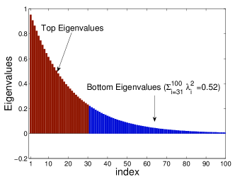
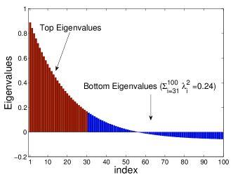
The following theorem shows an error bound of the SS model, which is stronger than the prototype model, especially when the bottom $n-k$ eigenvalues of ${\bf K}$ are big. The proof is in Appendix F.

Theorem 9

Suppose there is a sketching matrix ${\bf P}\in{\mathbb{R}}^{n\times c}$ such that for any $n\times n$ symmetric matrix ${\bf A}$ and target rank $k$ ($\ll n$), by forming the sketch ${\bf C}={\bf A}{\bf P}$, the prototype model satisfies the error bound

$$\big{\|}{\bf A}-{\bf C}{\bf C}^{\dagger}{\bf A}({\bf C}^{\dagger})^{T}{\bf C}^{T}\big{\|}_{F}^{2}\;\leq\;\eta\,\big{\|}{\bf A}-{\bf A}_{k}\big{\|}_{F}^{2}$$

for certain $\eta>0$. Let ${\bf K}$ be any $n\times n$ SPSD matrix, $\bar{\delta}$ defined in (11) be the initial spectral shifting term, and ${\tilde{{\bf K}}_{c}^{\textrm{ss}}}$ be the SS model defined in (10). Then

$$\big{\|}{\bf K}-{\tilde{{\bf K}}_{c}^{\textrm{ss}}}\big{\|}_{F}^{2}\>\leq\>\eta\bigg{(}\big{\|}{\bf K}-{\bf K}_{k}\big{\|}_{F}^{2}-\frac{\big{[}\sum_{i=k+1}^{n}\lambda_{i}({\bf K})\big{]}^{2}}{n-k}\bigg{)}.$$

If $\bar{\bf C}$ contains the columns of $\bar{{\bf K}}$ sampled by the near-optimal+adaptive algorithm in Theorem 3, which has the strongest bound, then the error bound incurred by SS is given in the following corollary.

Corollary 10

Suppose we are given any SPSD matrix ${\bf K}$ and we sample $c={\mathcal{O}}(k/\epsilon)$ columns of $\bar{{\bf K}}$ to form $\bar{{\bf C}}$ using the near-optimal+adaptive column sampling algorithm (Theorem 3). Then the inequality holds:

$${\mathbb{E}}\big{\|}{\bf K}-\tilde{{\bf K}}_{c}^{\textrm{ss}}\big{\|}_{F}^{2}\leq(1+\epsilon)\bigg{(}\|{\bf K}-{\bf K}_{k}\|_{F}^{2}-\frac{\big{[}\sum_{i=k+1}^{n}\lambda_{i}({\bf K})\big{]}^{2}}{n-k}\bigg{)}.$$

Here we give an example to demonstrate the superiority of SS over the prototype model, the Nyström method, and even the truncated SVD of the same scale.

Example 1

Let ${\bf K}$ be an $n\times n$ SPSD matrix such that $\lambda_{1}({\bf K})\geq\cdots\geq\lambda_{k}({\bf K})>\theta=\lambda_{k+1}({\bf K})=\cdots=\lambda_{n}({\bf K})>0$. By sampling $c={\mathcal{O}}(k)$ columns by the near-optimal+adaptive algorithm (Theorem 3), we have that

$$\big{\|}{\bf K}-\tilde{{\bf K}}_{c}^{\textrm{ss}}\big{\|}_{F}^{2}\;=\;0$$

and that

$$(n-c)\theta^{2}\;=\;\big{\|}{\bf K}-{\bf K}_{c}\big{\|}_{F}^{2}\;\leq\;\big{\|}{\bf K}-\tilde{{\bf K}}_{c}^{\textrm{proto}}\big{\|}_{F}^{2}\;\leq\;\big{\|}{\bf K}-\tilde{{\bf K}}_{c}^{\textrm{nys}}\big{\|}_{F}^{2}.$$

Here $\tilde{{\bf K}}_{c}^{\textrm{proto}}$ and $\tilde{{\bf K}}_{c}^{\textrm{nys}}$ respectively denote the approximation formed by the prototype model and the Nyström method. In this example the SS model is far better than the other models if we set $\theta$ as a large constant.

7.4 Approximately Computing $\bar{\delta}$

The SS model uses $\bar{\delta}$ as the initial spectral shifting term. However, computing $\bar{\delta}$ according to (11) requires the partial eigenvalue decomposition which costs ${\mathcal{O}}(n^{2}k)$ time and ${\mathcal{O}}(n^{2})$ memory. For large-scale data, one can simply set $\bar{\delta}=0$; Remark 7 shows that SS with this setting still works better than the prototype model. For medium-scale data, one can approximately compute $\bar{\delta}$ by the algorithm devised and analyzed in this subsection.

We depict the algorithm in Lines 2–6 of Algorithm 5. The performance of the approximation is analyzed in the following theorem.

Theorem 11

Let $\bar{\delta}$ be defined in (11) and $\tilde{\delta}$, $k$, $l$, $n$ be defined in Algorithm 5. The following inequality holds:

$${\mathbb{E}}\big{[}{\big{|}\bar{\delta}-\tilde{\delta}\big{|}}\,\big{/}\,{\bar{\delta}}\big{]}\;\leq\;{k}/{\sqrt{l}},$$

where the expectation is taken w.r.t. the Gaussian random matrix $\Omega$ in Algorithm 5. Lines 2–6 in Algorithm 5 compute $\tilde{\delta}$ in ${\mathcal{O}}(n^{2}l)$ time and ${\mathcal{O}}(nl)$ memory.

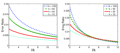
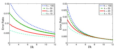
Here we empirically evaluate the accuracy of the approximation to $\bar{\delta}$ (Lines 2–6 in Algorithm 5) proposed in Theorem 11. We use the RBF kernel matrices with the scaling parameter $\gamma$ listed Table 3. We use the error ratio $|\bar{\delta}-\tilde{\delta}|/\bar{\delta}$ to evaluate the approximation quality. We repeat the experiments 20 times and plot $l/k$ against the average error ratio in Figure 7. Here $\tilde{\delta}$, $l$, and $k$ are defined in Theorem 11. We can see that the approximation of $\bar{\delta}$ has high quality: when $l=4k$, the error ratios are less than $0.03$ in all cases, no matter whether the spectrum of ${\bf K}$ decays fast or slow.

(a) Letters

(b) PenDigit

Figure 7: The ratio $\frac{l}{k}$ against the error $|\bar{\delta}-\tilde{\delta}|/\bar{\delta}$. In each subfigure, the left corresponds to the RBF kernel matrix with $\eta=0.5$, and the right corresponds to $\eta=0.9$, where $\eta$ is defined in (7).

7.5 Combining with Other Matrix Approximation Methods

There are many other matrix approximation approaches such as the ensemble Nyström method (Kumar et al., 2012) and MEKA (Si et al., 2014). In fact, the key components of the ensemble Nyström method and MEKA are the Nyström method, which can be straightforwardly replaced by other matrix approximation methods such as the SS model.

The ensemble Nyström method improves the Nyström method by running the Nyström method $t$ times and combine the samples to construct the kernel approximation:

$${\tilde{{\bf K}}_{t,c}^{\textrm{ens}}}\;=\;\sum_{i=1}^{t}\mu^{(i)}{\bf C}^{(i)}{{\bf W}^{(i)}}^{\dagger}{{\bf C}^{(i)}}^{T},$$

where $\mu^{(1)},\cdots,\mu^{(t)}$ are the weights of the samples, and a simple but effective strategy is to set the weights as $\mu^{(1)}=\cdots=\mu^{(t)}=\frac{1}{t}$. However, the time and memory costs of computing ${\bf C}$ and ${\bf U}$ are respectively $t$ times as much as that of its base method (e.g. the Nyström method), and the ensemble Nyström method needs to use the Sherman-Morrison-Woodbury formula $t$ times to combine the samples. When executed on a single machine, the accuracy gained by the ensemble may not worth the $t$ times more time and memory costs.

MEKA is reported to be the state-of-the-art kernel approximation method. It exploits the block-diagonal structure of kernel matrices, and outputs an ${n\times c}$ sparse matrix ${\bf C}$ and a $c\times c$ small matrix ${\bf U}$ such that ${\bf K}\approx{\bf C}{\bf U}{\bf C}^{T}$. MEKA first finds the blocks by clustering the data into $b$ clusters and permutes the kernel matrix accordingly. It then approximates the diagonal blocks by the Nyström method, which can be replaced by other methods. It finally approximates the off-diagonal blocks using the diagonal blocks. If the kernel matrix is partitioned into $b^{2}$ blocks, only $b$ blocks among the $b^{2}$ blocks of ${\bf C}$ are nonzero, and the number of nonzero entries of ${\bf C}$ is at most $\mathrm{nnz}({\bf C})=nc/b$. MEKA is thus much more memory efficient than the Nyström method. If we use the SS model to approximate the diagonal blocks, then the resulting MEKA approximation will be in the form ${\bf K}\approx{\bf C}{\bf U}{\bf C}^{T}+\delta_{1}{\bf I}\oplus\cdots\oplus\delta_{b}{\bf I}$, where $\delta_{i}$ corresponds to the $i$-th diagonal block.

Figure 8: The memory cost against approximation error. Here “nnz” is number of nonzero entries in the sketch, namely, $\mathrm{nnz}({\bf C})+\mathrm{nnz}({\bf U})$. In each subfigure, the left corresponds to the RBF kernel matrix with $\eta=0.5$, and the right corresponds to $\eta=0.9$, where $\eta$ is defined in (7).

Figure 9: The elapsed time (log-scale) against the approximation error. In each subfigure, the left corresponds to the RBF kernel matrix with $\eta=0.5$, and the right corresponds to $\eta=0.9$, where $\eta$ is defined in (7).

8 Empirically Evaluating the Spectral Shifting Model

We empirically evaluate the spectral shifting method by comparing the following kernel approximation models in terms of approximation quality and the generalization performance on Gaussian process regression.

• The Nyström method with the uniform+adaptive² algorithm.

• The prototype model with the uniform+adaptive² algorithm.

• The memory efficient kernel approximation (MEKA) method (Si et al., 2014), which approximates the diagonal blocks of the kernel matrix by the Nyström method. We use the code released by the authors with default settings.

• The spectral shifting (SS) model with the uniform+adaptive² algorithm.

• SS+MEKA: the same to MEKA except for using SS, rather than the Nyström method, to approximate the diagonal blocks.

Since the experiments are all done on a single machine, the time and memory costs of the ensemble Nyström method (Kumar et al., 2012) are $t$ times larger. It would be unfair to directly do comparison with the ensemble Nyström method.

(a) $\eta\approx 0.5$

(b) $\eta\approx 0.9$

Figure 10: The experiments on the covtype dataset. We plot the memory cost against approximation error and plot the elapsed time (log-scale) against the approximation error.

8.1 Experiments on Approximation Accuracy

We conduct experiments using the same setting as in Section 6.1. To demonstrate the effect of spectral shifting, we only consider a kernel matrix with slowly decaying spectrum. Thus we set $\eta$ (defined in (7)) relatively small: $\eta=0.5$ and $\eta=0.9$. When $\eta$ is near one, the spectral shifting term becomes near zero, and spectral shifting makes no difference.

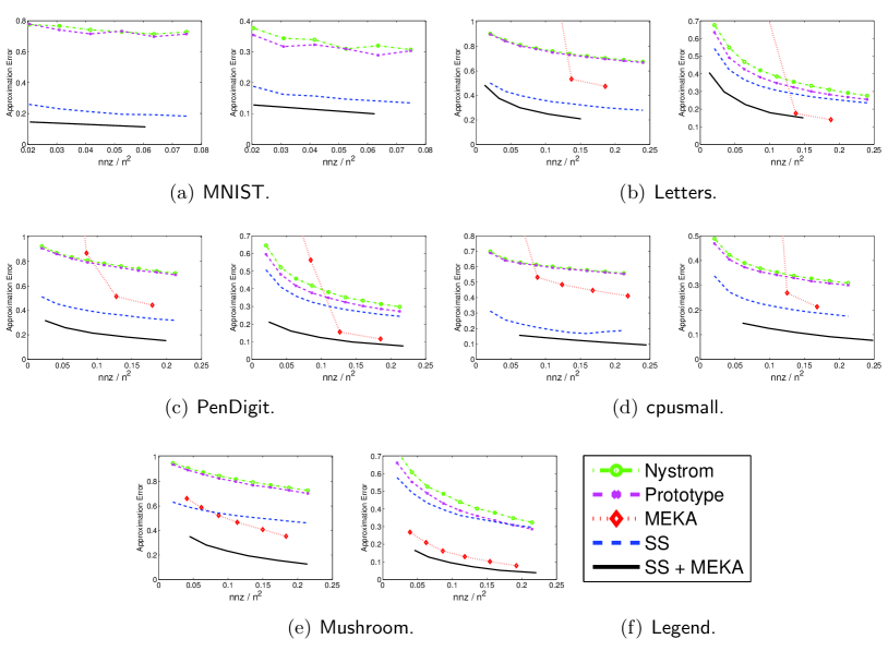
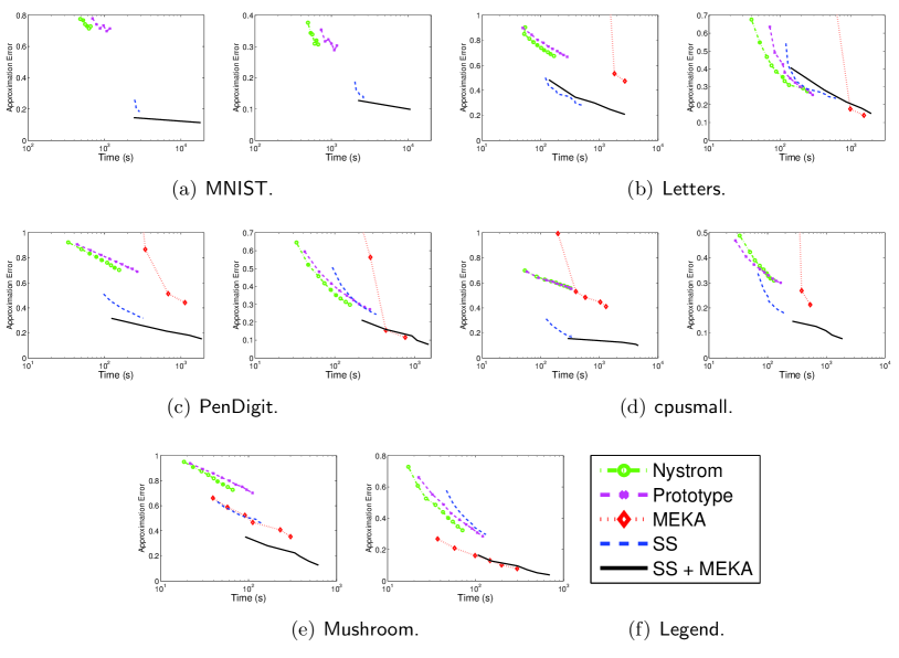
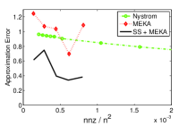
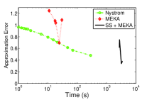
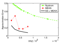
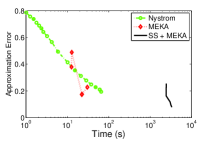
We present the results in two ways: (1) Figure 8 plots the memory usage against the approximation error, where the memory usage is proportional to the number of nonzero entries of ${\bf C}$ and ${\bf U}$; (2) Figure 9 plots the elapsed time against the approximation error. The results have the following implications.

• Using the spectral shifting technique is better than without using it: SS and SS+MEKA are more accurate than the prototype model and MEKA, respectively. The advantage of spectral shifting is particularly obvious when the spectrum of ${\bf K}$ decays slowly, i.e. when $\eta=0.5$.

• SS and SS+MEKA are the best among the compared methods according to our experiments. Especially, if a high-quality approximation in limited memory is desired, SS+MEKA should be the best choice.

• The kernel matrix of the MNIST dataset is $60,000\times 60,000$, which does not fit in the $24$GB memory. This shows that the compared methods and sampling algorithm do not require keeping ${\bf K}$ in memory.

In addition, we conduct experiments on the large-scale dataset—covtype—which has 581,012 data instances. We compare among the Nyström method, MEKA, and MEKA+SS. The experiment setting is slightly different from the ones in the above. For each of the four methods, we use uniform sampling to select columns. As for the MEKA based methods, we set the number of clusters to be 30 (whereas the default is 10) to increase scalability. As for the spectral shifting method, we do not perform the initial spectral shifting. The results are plotted in Figure 10. The results show the effectiveness and scalability of the spectral shift method.

Table 4: Summary of datasets for Gaussian process regression

	Plant	White Wine	Red Wine	Concrete	Energy (Heat)	Energy (Cool)	Housing
#Instance	9,568	4,898	1,599	1,030	768	768	506
#Attribute	4	11	11	8	8	8	13
$\gamma$	0.1	1	1	1	0.5	0.5	1
$\sigma^{2}$	0.1	0.01	0.01	0.0002	0.0005	0.001	0.005

8.2 Experiments on Gaussian Process Regression

We apply the kernel approximation methods to Gaussian process regression (GPR). We assume that the training set is $\{({\bf x}_{1},y_{1}),...,({\bf x}_{n},y_{n})\}$, where ${\bf x}_{i}\in{\mathbb{R}}^{d}$ are input vectors and $y_{i}\in{\mathbb{R}}$ are the corresponding outputs. GPR is defined as

$$y=u+f({\bf x})+\epsilon,\quad\epsilon\sim\mathcal{N}(0,\sigma^{2}),$$

where $f({\bf x})$ follows a Gaussian process with mean function 0 and kernel function $\kappa(\cdot,\cdot)$. Furthermore, we define the kernel matrix ${\bf K}\in{\mathbb{R}}^{n\times n}$, where the $(i,j)$-th entry of ${\bf K}$ is $\kappa({\bf x}_{i},{\bf x}_{j})$.

For a test input ${\bf x}_{*}$, the prediction is given by

$$\hat{y}_{*}={\bf k}^{T}({\bf x}_{*})({\bf K}+\sigma^{2}{\bf I})^{-1}{\bf y},$$

where ${\bf y}=[y_{1},\dots,y_{n}]^{T}$ and ${\bf k}({\bf x}_{*})=[\kappa({\bf x}_{*},{\bf x}_{1}),\dots,\kappa({\bf x}_{*},{\bf x}_{n})]^{T}$. We apply different kernel approximation methods to approximate ${\bf K}$ and approximately compute $({\bf K}+\sigma^{2}{\bf I})^{-1}{\bf y}$ according to Section 3.1. We evaluate the generalization performance using the mean squared error:

$$\mbox{MSE}=\frac{1}{m}\sum_{i=1}^{m}(y_{i*}-{\hat{y}}_{i*})^{2},$$

where $y_{i*}$ is the real output of the $i$-th test sample and $m$ is the number of test samples.

Figure 11: The results on Gaussian process regression. In the figures “nnz” is number of nonzero entries in the sketch, that is, $\mathrm{nnz}({\bf C})+\mathrm{nnz}({\bf U})$.

Figure 12: The results on Gaussian process regression.

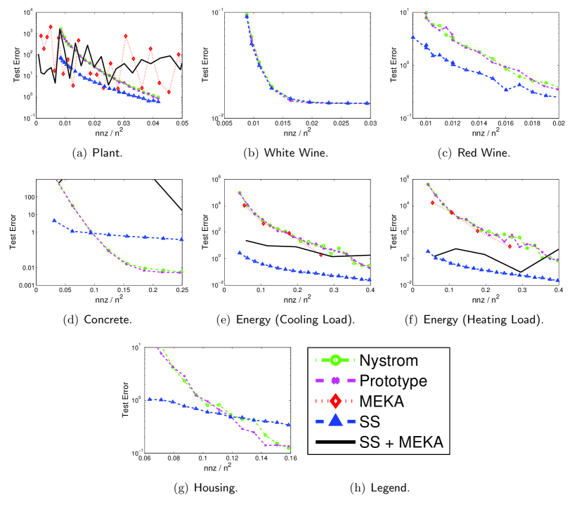
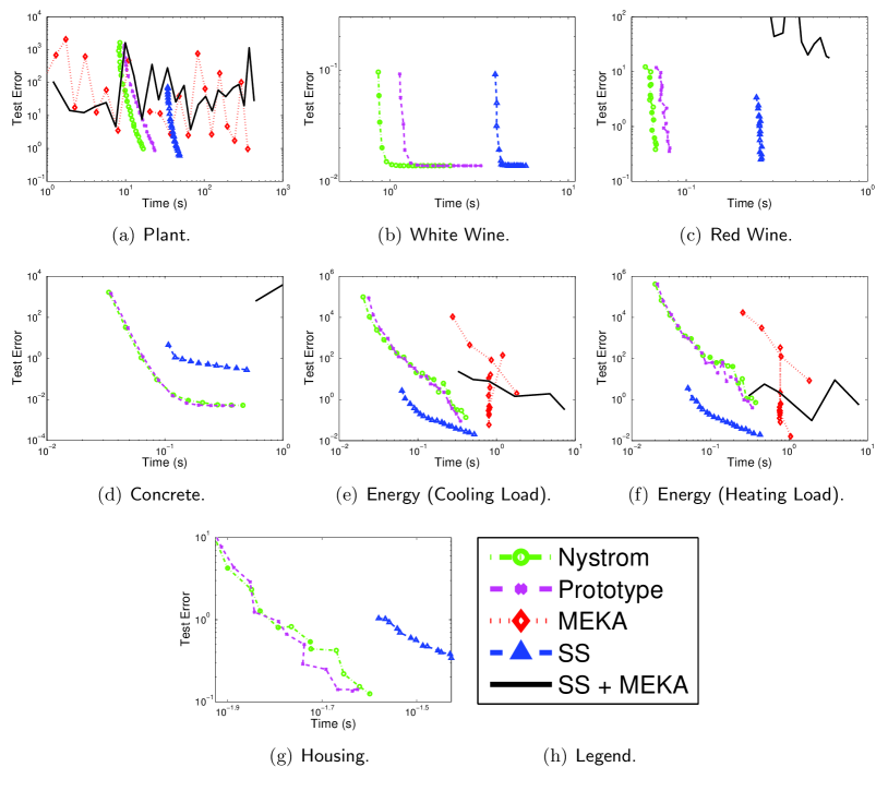
We conduct experiment on seven datasets summarized in Table 4. We use the Gaussian RBF kernel and tune two parameters: the variance $\sigma^{2}$ and the kernel scaling parameter $\gamma$. Recall that there are seven compared methods and eight datasets, so the time cost would be daunting if we use cross-validation to find $\sigma$ and $\gamma$ for each method on each dataset. Thus we perform a five-fold cross-validation without using kernel approximation to pre-determine the two parameters $\sigma$ and $\gamma$, and the same parameters are used for all the kernel approximation methods. We list the obtained parameters in Table 4.

For each of the compared methods, we randomly hold $80\%$ samples for training and the rest for test; we repeat this procedure $50$ times and record the average MSE, the average elapsed time, and the average of the number of nonzero entries in the sketch. We plot $\frac{\mathrm{nnz}({\bf C})+\mathrm{nnz}({\bf U})}{n^{2}}$ against MSE in Figure 11 and the elapsed time against MSE in Figure 12.

Using the same amount of memory, our SS model achieves the best performance on the Plant, Red Wine, Energy (Cool), and Energy (Heat) datasets. On the Concrete and Housing datasets, using spectral shifting leads better results unless $c$ is unreasonably large (e.g.  $c>0.1n$). However, using the same amount of time, the compared methods have competitive performance.

MEKA and SS+MEKA in general work very well, but they are numerically unstable on some of the randomly partitioned training data. On the White Wine, Housing, and Concrete datasets, MATLAB occasionally reports errors of numerical instability in approximating the off-diagonal blocks of ${\bf K}$ by solving some linear systems; when such happens, we do not report the corresponding test errors in the figures. MEKA and SS+MEKA are also sometimes unstable on the Plant and Red Wine datasets, though MATLAB does not report error. Although MEKA and SS+MEKA have good performance in general, the numerical instability makes MEKA and SS+MEKA perform very poorly on a few among the 50 randomly partitioned training/test data, and consequently the average test errors become large. This problem can get avoided by repeating MEKA multiple times and choose the one that is stable. However, this will significantly increase the time cost.

9 Conclusions

We have provided an in-depth study of the prototype model for SPSD matrix approximation. First, we have shown that with $c={\mathcal{O}}(k/\epsilon)$ columns sampled by the near-optimal+adaptive algorithm, the prototype model attains $1+\epsilon$ Frobenius norm relative-error bound. This upper bound matches the lower bound up to a constant factor. Second, we have devised a simple column selection algorithm called uniform+adaptive². The algorithm is efficient and very easy to implement, and it has near-optimal relative-error bound. Third, we have proposed an extension called the spectral shifting (SS) model. We have shown that SS has much stronger error bound than the low-rank approximation models, especially when the bottom eigenvalues are not sufficiently small.

Although the prototype model is not very time-efficient, we can resort to the approximate method provided by Wang et al. (2015) to obtain a faster solution to the prototype model. This faster solution requires only linear time and linear memory. The theoretical analysis of the fast solution heavily relies on that of the prototype model, so our established results are useful even if the prototype model itself is not the working horse in real-world applications. In addition, we have shown that the fast solution can also be naturally incorporated with the spectral shifting method.

Acknowledgments

We thank the anonymous reviewers for their helpful suggestions. Wang has been supported by Baidu Scholarship. Luo and Zhang have been supported by the National Natural Science Foundation of China (No. 61572017), Natural Science Foundation of Shanghai City (No. 15ZR1424200), and Microsoft Research Asia Collaborative Research Award.

A Proof of Theorem 1

Proof  Suppose that $\mathrm{rank}({\bf W})=\mathrm{rank}({\bf K})$. We have that $\mathrm{rank}({\bf W})=\mathrm{rank}({\bf C})=\mathrm{rank}({\bf K})$ because

$$\mathrm{rank}({\bf K})\;\geq\;\mathrm{rank}({\bf C})\;\geq\;\mathrm{rank}({\bf W})\textrm{.}$$ (15)

Thus there exists a matrix ${\bf X}$ such that

$$\left[\begin{array}[]{c}{\bf K}_{21}^{T}\\ {\bf K}_{22}\\ \end{array}\right]\;=\;{\bf C}{\bf X}^{T}\;=\;\left[\begin{array}[]{c}{\bf W}{\bf X}^{T}\\ {\bf K}_{21}{\bf X}^{T}\\ \end{array}\right]\textrm{,}$$

and it follows that ${\bf K}_{21}={\bf X}{\bf W}$ and ${\bf K}_{22}={\bf K}_{21}{\bf X}^{T}={\bf X}{\bf W}{\bf X}^{T}$. Then we have that

$${\bf K} = \left[\begin{array}[]{cc}{\bf W}&({\bf X}{\bf W})^{T}\\ {\bf X}{\bf W}&{\bf X}{\bf W}{\bf X}^{T}\\ \end{array}\right]\;=\;\left[\begin{array}[]{c}{\bf I}\\ {\bf X}\\ \end{array}\right]{\bf W}\left[\begin{array}[]{cc}{\bf I}&{\bf X}^{T}\\ \end{array}\right]\textrm{,}$$ (21)

$${\bf C}{\bf W}^{\dagger}{\bf C}^{T} = \left[\begin{array}[]{c}{\bf W}\\ {\bf X}{\bf W}\\ \end{array}\right]{\bf W}^{\dagger}\left[\begin{array}[]{cc}{\bf W}&({\bf X}{\bf W})^{T}\\ \end{array}\right]\;=\;\left[\begin{array}[]{c}{\bf I}\\ {\bf X}\\ \end{array}\right]{\bf W}\left[\begin{array}[]{cc}{\bf I}&{\bf X}^{T}\\ \end{array}\right]\textrm{.}$$ (28)

Here the second equality in (28) follows from ${\bf W}{\bf W}^{\dagger}{\bf W}={\bf W}$. We obtain that ${\bf K}={\bf C}{\bf W}^{\dagger}{\bf C}$. Then we show that ${\bf K}={\bf C}{\bf C}^{\dagger}{\bf K}({\bf C}^{\dagger})^{T}{\bf C}^{T}$.

Since ${\bf C}^{\dagger}=({\bf C}^{T}{\bf C})^{\dagger}{\bf C}^{T}$, we have that

$${\bf C}^{\dagger}\;=\;\big{(}{\bf W}({\bf I}+{\bf X}^{T}{\bf X}){\bf W}\big{)}^{\dagger}{\bf W}\>[{\bf I}\,,\,{\bf X}^{T}]\textrm{,}$$

and thus

$${\bf C}^{\dagger}{\bf K}({\bf C}^{\dagger})^{T}{\bf W}$$

$$=\;\big{(}{\bf W}({\bf I}+{\bf X}^{T}{\bf X}){\bf W}\big{)}^{\dagger}{\bf W}({\bf I}+{\bf X}^{T}{\bf X})\Big{[}{\bf W}({\bf I}+{\bf X}^{T}{\bf X}){\bf W}\big{(}{\bf W}({\bf I}+{\bf X}^{T}{\bf X}){\bf W}\big{)}^{\dagger}{\bf W}\Big{]}$$

$$=\;\big{(}{\bf W}({\bf I}+{\bf X}^{T}{\bf X}){\bf W}\big{)}^{\dagger}{\bf W}({\bf I}+{\bf X}^{T}{\bf X}){\bf W}\textrm{,}$$

where the second equality follows from Lemma 12 because $({\bf I}+{\bf X}^{T}{\bf X})$ is positive definite. Similarly we have

$${\bf W}{\bf C}^{\dagger}{\bf K}({\bf C}^{\dagger})^{T}{\bf W}\;=\;{\bf W}\big{(}{\bf W}({\bf I}+{\bf X}^{T}{\bf X}){\bf W}\big{)}^{\dagger}{\bf W}({\bf I}+{\bf X}^{T}{\bf X}){\bf W}\;=\;{\bf W}\textrm{.}$$

Thus we have

$${\bf C}{\bf C}^{\dagger}{\bf K}({\bf C}^{\dagger})^{T}{\bf C}\;=\;\left[\begin{array}[]{c}{\bf I}\\ {\bf X}\\ \end{array}\right]{\bf W}{\bf C}^{\dagger}{\bf K}({\bf C}^{\dagger})^{T}{\bf W}\left[\begin{array}[]{cc}{\bf I}&{\bf X}^{T}\\ \end{array}\right]\;=\;\left[\begin{array}[]{c}{\bf I}\\ {\bf X}\\ \end{array}\right]{\bf W}\left[\begin{array}[]{cc}{\bf I}&{\bf X}^{T}\\ \end{array}\right]\textrm{.}$$ (35)

It follows from Equations (21) (28) (35) that ${\bf K}={\bf C}{\bf W}^{\dagger}{\bf C}^{T}={\bf C}{\bf C}^{\dagger}{\bf K}({\bf C}^{\dagger})^{T}{\bf C}^{T}$.

Conversely, when ${\bf K}={\bf C}{\bf W}^{\dagger}{\bf C}^{T}$, it holds that $\mathrm{rank}({\bf K})\leq\mathrm{rank}({\bf W}^{\dagger})=\mathrm{rank}({\bf W})$. It follows from (15) that $\mathrm{rank}({\bf K})=\mathrm{rank}({\bf W})$.

When ${\bf K}={\bf C}{\bf C}^{\dagger}{\bf K}({\bf C}^{\dagger})^{T}{\bf C}^{T}$, we have $\mathrm{rank}({\bf K})\leq\mathrm{rank}({\bf C})$. Thus there exists a matrix ${\bf X}$ such that

$$\left[\begin{array}[]{c}{\bf K}_{21}^{T}\\ {\bf K}_{22}\\ \end{array}\right]\;=\;{\bf C}{\bf X}^{T}\;=\;\left[\begin{array}[]{c}{\bf W}{\bf X}^{T}\\ {\bf K}_{21}{\bf X}^{T}\\ \end{array}\right]\textrm{,}$$

and therefore ${\bf K}_{21}={\bf X}{\bf W}$. Then we have that

$${\bf C}\;=\;\left[\begin{array}[]{c}{\bf W}\\ {\bf K}_{21}\\ \end{array}\right]\;=\;\left[\begin{array}[]{c}{\bf I}\\ {\bf X}\\ \end{array}\right]{\bf W}\textrm{,}$$

so $\mathrm{rank}({\bf C})\leq\mathrm{rank}({\bf W})$. Apply (15) again we have $\mathrm{rank}({\bf K})=\mathrm{rank}({\bf W})$.  

Lemma 12

${\bf X}^{T}{\bf V}{\bf X}\big{(}{\bf X}^{T}{\bf V}{\bf X}\big{)}^{\dagger}{\bf X}^{T}={\bf X}^{T}$ for any positive definite matrix ${\bf V}$.

Proof  The positive definite matrix ${\bf V}$ have a decomposition ${\bf V}={\bf B}^{T}{\bf B}$ for some nonsingular matrix ${\bf B}$. It follows that

$${\bf X}^{T}{\bf V}{\bf X}\big{(}{\bf X}^{T}{\bf V}{\bf X}\big{)}^{\dagger}{\bf X}^{T} = ({\bf B}{\bf X})^{T}\Big{(}{\bf B}{\bf X}\big{(}({\bf B}{\bf X})^{T}({\bf B}{\bf X})\big{)}^{\dagger}\Big{)}({\bf B}{\bf X})^{T}{\bf B}({\bf B}^{T}{\bf B})^{-1}$$

$$= ({\bf B}{\bf X})^{T}\big{(}({\bf B}{\bf X})^{T}\big{)}^{{\dagger}}({\bf B}{\bf X})^{T}({\bf B}^{T})^{-1}\;=\;({\bf B}{\bf X})^{T}({\bf B}^{T})^{-1}\;=\;{\bf X}^{T}\textrm{.}$$

 

B Proof of Theorem 2

In Section B.1 we provide several key lemmas, and then in Section B.2 we prove Theorem 2 using Lemmas 14 and 15.

B.1 Key Lemmas

Lemma 13 provides a useful tool for expanding the Moore-Penrose inverse of partitioned matrices, and the lemma will be used to prove Lemma 15 and Theorem 2.

Lemma 13

(see Ben-Israel and Greville, 2003, Page 179) Given a matrix ${\bf X}\in{{\mathbb{R}}^{m\times n}}$ of rank $c$, let it have a nonsingular $c\times c$ submatrix ${\bf X}_{11}$. By rearrangement of columns and rows by permutation matrices ${\bf P}$ and ${\bf Q}$, the submatrix ${\bf X}_{11}$ can be bought to the top left corner of ${\bf X}$, that is,

$${\bf P}{\bf X}{\bf Q}\;=\;\left[\begin{array}[]{cc}{\bf X}_{11}&{\bf X}_{12}\\ {\bf X}_{21}&{\bf X}_{22}\\ \end{array}\right].$$

Then the Moore-Penrose inverse of ${\bf X}$ is

$${\bf X}^{\dagger}\;=\;{\bf Q}\left[\begin{array}[]{c}{\bf I}_{c}\\ {\bf T}^{T}\\ \end{array}\right]\big{(}{\bf I}_{c}+{\bf T}{\bf T}^{T}\big{)}^{-1}{\bf X}_{11}^{-1}\big{(}{\bf I}_{c}+{\bf S}^{T}{\bf S}\big{)}^{-1}\left[\begin{array}[]{cc}{\bf I}_{c}&{\bf S}^{T}\\ \end{array}\right]{\bf P},$$ (39)

where ${\bf T}={\bf X}_{11}^{-1}{\bf X}_{12}$ and ${\bf S}={\bf X}_{21}{\bf X}_{11}^{-1}$.

Lemmas 14 and 15 will be used to prove Theorem 2.

Lemma 14

(Wang and Zhang, 2013, Lemma 19) Given $n$ and $k$, we let ${\bf B}$ be an $\frac{n}{k}\times\frac{n}{k}$ matrix whose diagonal entries equal to one and off-diagonal entries equal to $\alpha\in[0,1)$. Let ${\bf A}$ be the $n\times n$ block-diagonal matrix

$${\bf A}\;=\;\underbrace{{\bf B}\oplus{\bf B}\oplus\cdots\oplus{\bf B}}_{k\textrm{ blocks}}.$$ (40)

Let ${\bf A}_{k}$ be the best rank-$k$ approximation to ${\bf A}$. Then

$$\|{\bf A}-{\bf A}_{k}\|_{F}\;=\;(1-\alpha)\sqrt{n-k}\textrm{.}$$

Lemma 15

Let ${\bf B}$ be the $n\times n$ matrix with diagonal entries equal to one and off-diagonal entries equal to $\alpha$ and $\tilde{\bf B}$ be its rank $c$ approximation formed by the prototype model. Then

$$\|{\bf B}-\tilde{{\bf B}}\|_{F}^{2}\;\geq\;(1-\alpha)^{2}(n-c)\bigg{(}1+\frac{2}{c}-(1-\alpha)\frac{1+o(1)}{\alpha cn/2}\bigg{)}\textrm{.}$$

Proof  Without loss of generality, we assume the first $c$ column of ${\bf B}$ are selected to construct ${\bf C}$. We partition ${\bf B}$ and ${\bf C}$ as:

$${\bf B}=\left[\begin{array}[]{cc}{\bf W}&{\bf B}_{21}^{T}\\ {\bf B}_{21}&{\bf B}_{22}\\ \end{array}\right]\qquad\textrm{ and }\qquad{\bf C}=\left[\begin{array}[]{c}{\bf W}\\ {\bf B}_{21}\\ \end{array}\right]\textrm{.}$$

Here the matrix ${\bf W}$ can be expressed by ${\bf W}=(1-\alpha){\bf I}_{c}+\alpha{\bf 1}_{c}{\bf 1}_{c}^{T}$. We apply the Sherman-Morrison-Woodbury matrix identity

$$({\bf X}+{\bf Y}{\bf Z}{\bf R})^{-1}={\bf X}^{-1}-{\bf X}^{-1}{\bf Y}({\bf Z}^{-1}+{\bf R}{\bf X}^{-1}{\bf Y})^{-1}{\bf R}{\bf X}^{-1}$$

to compute ${\bf W}^{-1}$, and it follows that

$${\bf W}^{-1}\;=\;\frac{1}{1-\alpha}{\bf I}_{c}-\frac{\alpha}{(1-\alpha)(1-\alpha+c\alpha)}{\bf 1}_{c}{\bf 1}_{c}^{T}\textrm{.}$$ (41)

We expand the Moore-Penrose inverse of ${\bf C}$ by Lemma 13 and obtain

$${\bf C}^{\dagger}={\bf W}^{-1}\big{(}{\bf I}_{c}+{\bf S}^{T}{\bf S}\big{)}^{-1}\left[\begin{array}[]{cc}{\bf I}_{c}&{\bf S}^{T}\\ \end{array}\right]$$

where

$${\bf S}={\bf B}_{21}{\bf W}^{-1}=\frac{\alpha}{1-\alpha+c\alpha}{\bf 1}_{n-c}{\bf 1}_{c}^{T}.$$

It is easily verified that ${\bf S}^{T}{\bf S}=\big{(}\frac{\alpha}{1-\alpha+c\alpha}\big{)}^{2}(n-c){\bf 1}_{c}{\bf 1}_{c}^{T}$.

Now we express the approximation by the prototype model in the partitioned form:

$$\tilde{{\bf B}}\;=\;{\bf C}{\bf C}^{\dagger}{\bf B}\big{(}{\bf C}^{\dagger}\big{)}^{T}{\bf C}^{T}$$

$$=\;\left[\begin{array}[]{c}{\bf W}\\ {\bf B}_{21}\\ \end{array}\right]{\bf W}^{-1}\big{(}{\bf I}_{c}+{\bf S}^{T}{\bf S}\big{)}^{-1}\left[\begin{array}[]{c c}{\bf I}_{c}&{\bf S}^{T}\\ \end{array}\right]{\bf B}\left[\begin{array}[]{c}{\bf I}_{c}\\ {\bf S}\\ \end{array}\right]\big{(}{\bf I}_{c}+{\bf S}^{T}{\bf S}\big{)}^{-1}{\bf W}^{-1}\left[\begin{array}[]{c}{\bf W}\\ {\bf B}_{21}\\ \end{array}\right]^{T}$$ (49)

$$=\;\left[\begin{array}[]{c}\big{(}{\bf I}_{c}+{\bf S}^{T}{\bf S}\big{)}^{-1}\\ {\bf B}_{21}{\bf W}^{-1}\big{(}{\bf I}_{c}+{\bf S}^{T}{\bf S}\big{)}^{-1}\\ \end{array}\right]\left[\begin{array}[]{c c}{\bf I}_{c}&{\bf S}^{T}\\ \end{array}\right]{\bf B}\left[\begin{array}[]{c}{\bf I}_{c}\\ {\bf S}\\ \end{array}\right]\left[\begin{array}[]{c}\big{(}{\bf I}_{c}+{\bf S}^{T}{\bf S}\big{)}^{-1}\\ {\bf B}_{21}{\bf W}^{-1}\big{(}{\bf I}_{c}+{\bf S}^{T}{\bf S}\big{)}^{-1}\\ \end{array}\right]^{T}\textrm{.}$$ (57)

We then compute the submatrices $\big{(}{\bf I}_{c}+{\bf S}^{T}{\bf S}\big{)}^{-1}$ and ${\bf B}_{21}{\bf W}^{-1}\big{(}{\bf I}_{c}+{\bf S}^{T}{\bf S}\big{)}^{-1}$ respectively as follows. We apply the Sherman-Morrison-Woodbury matrix identity to compute $\big{(}{\bf I}_{c}+{\bf S}^{T}{\bf S}\big{)}^{-1}$. We obtain

$$\big{(}{\bf I}_{c}+{\bf S}^{T}{\bf S}\big{)}^{-1}\;=\;\bigg{(}{\bf I}_{c}+\Big{(}\frac{\alpha}{1-\alpha+c\alpha}\Big{)}^{2}(n-c){\bf 1}_{c}{\bf 1}_{c}^{T}\bigg{)}^{-1}\;=\;{\bf I}_{c}-\gamma_{1}{\bf 1}_{c}{\bf 1}_{c}^{T}\textrm{,}$$ (58)

where

$$\gamma_{1}=\frac{n-c}{nc+\big{(}\frac{1-\alpha}{\alpha}\big{)}^{2}+\frac{2(1-\alpha)c}{\alpha}}.$$

It follows from (41) and (58) that

$${\bf W}^{-1}\big{(}{\bf I}_{c}+{\bf S}^{T}{\bf S}\big{)}^{-1}\;=\;(\gamma_{2}{\bf I}_{c}-\gamma_{3}{\bf 1}_{c}{\bf 1}_{c}^{T})({\bf I}_{c}-\gamma_{1}{\bf 1}_{c}{\bf 1}_{c}^{T})\;=\;\gamma_{2}{\bf I}_{c}+(\gamma_{1}\gamma_{3}c-\gamma_{1}\gamma_{2}-\gamma_{3}){\bf 1}_{c}{\bf 1}_{c}^{T},$$

where

$$\gamma_{2}=\frac{1}{1-\alpha}\quad\textrm{ and }\quad\gamma_{3}=\frac{\alpha}{(1-\alpha)(1-\alpha+\alpha c)}.$$

It follows that

$${\bf B}_{21}{\bf W}^{-1}\big{(}{\bf I}_{c}+{\bf S}^{T}{\bf S}\big{)}^{-1}\;=\;\alpha\big{(}\gamma_{1}\gamma_{3}c^{2}-\gamma_{3}c-\gamma_{1}\gamma_{2}c+\gamma_{2}\big{)}{\bf 1}_{n-c}{\bf 1}_{c}^{T}\;\triangleq\;\gamma{\bf 1}_{n-c}{\bf 1}_{c}^{T},$$ (59)

where

$$\gamma = \alpha\big{(}\gamma_{1}\gamma_{3}c^{2}-\gamma_{3}c-\gamma_{1}\gamma_{2}c+\gamma_{2}\big{)}\;=\;\frac{\alpha(\alpha c-\alpha+1)}{2\alpha c-2\alpha-2\alpha^{2}c+\alpha^{2}+\alpha^{2}cn+1}\textrm{.}$$ (60)

Since ${\bf B}_{21}=\alpha{\bf 1}_{n-c}{\bf 1}_{c}^{T}$ and ${\bf B}_{22}=(1-\alpha){\bf I}_{n-c}+\alpha{\bf 1}_{n-c}{\bf 1}_{n-c}^{T}$, it is easily verified that

$$\left[\begin{array}[]{cc}{\bf I}_{c}&{\bf S}^{T}\\ \end{array}\right]{\bf B}\left[\begin{array}[]{c}{\bf I}_{c}\\ {\bf S}\\ \end{array}\right]\;=\;\left[\begin{array}[]{cc}{\bf I}_{c}&{\bf S}^{T}\\ \end{array}\right]\left[\begin{array}[]{cc}{\bf W}&{\bf B}_{21}^{T}\\ {\bf B}_{21}&{\bf B}_{22}\\ \end{array}\right]\left[\begin{array}[]{c}{\bf I}_{c}\\ {\bf S}\\ \end{array}\right]\;=\;(1-\alpha){\bf I}_{c}+\lambda{\bf 1}_{c}{\bf 1}_{c}^{T}\textrm{,}$$ (69)

where

$$\lambda=\frac{\alpha(3\alpha n-\alpha c-2\alpha+\alpha^{2}c-3\alpha^{2}n+\alpha^{2}+\alpha^{2}n^{2}+1)}{(\alpha c-\alpha+1)^{2}}$$

It follows from (57), (58), (59), and (69) that

$$\tilde{{\bf B}}\;=\;\left[\begin{array}[]{c}{\bf I}_{c}-\gamma_{1}{\bf 1}_{c}{\bf 1}_{c}^{T}\\ \gamma{\bf 1}_{n-c}{\bf 1}_{c}^{T}\\ \end{array}\right]\Big{(}(1-\alpha){\bf I}_{c}+\lambda{\bf 1}_{c}{\bf 1}_{c}^{T}\Big{)}\left[\begin{array}[]{c}{\bf I}_{c}-\gamma_{1}{\bf 1}_{c}{\bf 1}_{c}^{T}\\ \gamma{\bf 1}_{n-c}{\bf 1}_{c}^{T}\\ \end{array}\right]^{T}\;\triangleq\;\left[\begin{array}[]{cc}\tilde{{\bf B}}_{11}&\tilde{{\bf B}}_{21}^{T}\\ \tilde{{\bf B}}_{21}&\tilde{{\bf B}}_{22}\\ \end{array}\right],$$ (76)

where

$$\tilde{{\bf B}}_{11} = (1-\alpha){\bf I}_{c}+\big{[}(1-\gamma_{1}c)(\lambda-\lambda\gamma_{1}c-(1-\alpha)\gamma_{1})-(1-\alpha)\gamma_{1}\big{]}{\bf 1}_{c}{\bf 1}_{c}^{T}$$

$$= (1-\alpha){\bf I}_{c}+\eta_{1}{\bf 1}_{c}{\bf 1}_{c}^{T},$$

$$\tilde{{\bf B}}_{21} = \tilde{{\bf A}}_{12}^{T}\;=\;\gamma(1-\gamma_{1}c)(1-\alpha+\lambda c){\bf 1}_{n-c}{\bf 1}_{c}^{T}\;=\;\eta_{2}{\bf 1}_{n-c}{\bf 1}_{c}^{T},$$

$$\tilde{{\bf B}}_{22} = \gamma^{2}c(1-\alpha+\lambda c){\bf 1}_{n-c}{\bf 1}_{n-c}^{T}\;=\;\eta_{3}{\bf 1}_{n-c}{\bf 1}_{n-c}^{T},$$

where

$$\eta_{1} = (1-\gamma_{1}c)(\lambda-\lambda\gamma_{1}c-(1-\alpha)\gamma_{1})-(1-\alpha)\gamma_{1},$$

$$\eta_{2} = \gamma(1-\gamma_{1}c)(1-\alpha+\lambda c),$$

$$\eta_{3} = \gamma^{2}c(1-\alpha+\lambda c),$$

By dealing with the four blocks of $\tilde{{\bf B}}$ respectively, we finally obtain that

$$\|{\bf B}-\tilde{{\bf B}}\|_{F}^{2} = \|{\bf W}-\tilde{{\bf B}}_{11}\|_{F}^{2}+2\|{\bf B}_{21}-\tilde{{\bf B}}_{21}\|_{F}^{2}+\|{\bf B}_{22}-\tilde{{\bf B}}_{22}\|_{F}^{2}$$

$$= c^{2}(\alpha-\eta_{1})^{2}+2c(n-c)(\alpha-\eta_{2})^{2}$$

$$+(n-c)(n-c-1)(\alpha-\eta_{3})^{2}+(n-c)(1-\eta_{3})^{2}$$

$$= (n-c)(\alpha-1)^{2}\bigg{(}1+\frac{2}{c}-\big{(}1+o(1)\big{)}\frac{1-\alpha}{\alpha cn/2}\bigg{)}\textrm{.}$$

 

B.2 Proof of the Theorem

Now we prove Theorem 2 using Lemma 15 and Lemma 14. Let ${\bf C}$ consist of $c$ columns sampled from ${\bf A}$ and $\hat{{\bf C}}_{i}$ consist of $c_{i}$ columns sampled from the $i$-th block diagonal matrix in ${\bf A}$. Without loss of generality, we assume $\hat{{\bf C}}_{i}$ consists of the first $c_{i}$ columns of ${\bf B}$. Then the intersection matrix ${\bf U}$ is computed by

$${\bf U} = {\bf C}^{\dagger}{\bf A}\big{(}{\bf C}^{T}\big{)}^{\dagger}\;=\;\big{[}\hat{{\bf C}}_{1}\oplus\cdots\oplus\hat{{\bf C}}_{k}\big{]}^{\dagger}\big{[}{\bf B}\oplus\cdots\oplus{\bf B}\big{]}\big{[}\hat{{\bf C}}_{1}^{T}\oplus\cdots\oplus\hat{{\bf C}}_{k}^{T}\big{]}^{\dagger}$$

$$= \hat{{\bf C}}_{1}^{\dagger}{\bf B}\big{(}\hat{{\bf C}}_{1}^{\dagger}\big{)}^{T}\oplus\cdots\oplus\hat{{\bf C}}_{k}^{\dagger}{\bf B}\big{(}\hat{{\bf C}}_{k}^{\dagger}\big{)}^{T}\textrm{.}$$

Let $\tilde{\bf A}$ be the approximation formed by the prototype model. Then

$$\tilde{{\bf A}}\;=\;{\bf C}{\bf U}{\bf C}^{T}\;=\;\hat{{\bf C}}_{1}\hat{{\bf C}}_{1}^{\dagger}{\bf B}\big{(}\hat{{\bf C}}_{1}^{\dagger}\big{)}^{T}\hat{{\bf C}}_{1}^{T}\oplus\cdots\oplus\hat{{\bf C}}_{k}\hat{{\bf C}}_{k}^{\dagger}{\bf B}\big{(}\hat{{\bf C}}_{k}^{\dagger}\big{)}^{T}\hat{{\bf C}}_{k}^{T}\textrm{,}$$

and thus the approximation error is

$$\big{\|}{\bf A}-\tilde{{\bf A}}\big{\|}_{F}^{2} = \sum_{i=1}^{k}\Big{\|}{\bf B}\;-\;\hat{{\bf C}}_{i}\hat{{\bf C}}_{i}^{\dagger}{\bf B}\big{(}\hat{{\bf C}}_{i}^{\dagger}\big{)}^{T}\hat{{\bf C}}_{i}^{T}\Big{\|}_{F}^{2}$$

$$\geq (1-\alpha)^{2}\sum_{i=1}^{k}(p-c_{i})\bigg{(}1+\frac{2}{c_{i}}-(1-\alpha)\Big{(}\frac{1+o(1)}{\alpha c_{i}p/2}\Big{)}\bigg{)}$$

$$= (1-\alpha)^{2}\bigg{(}\sum_{i=1}^{k}(p-c_{i})+\sum_{i=1}^{k}\frac{2(p-c_{i})}{c_{i}}\Big{(}1-\frac{(1-\alpha)(1+o(1))}{\alpha p}\Big{)}\bigg{)}$$

$$\geq (1-\alpha)^{2}(n-c)\bigg{(}1+\frac{2k}{c}\Big{(}1-\frac{k(1-\alpha)(1+o(1))}{\alpha n}\Big{)}\bigg{)}\textrm{,}$$

where the former inequality follows from Lemma 15, and the latter inequality follows by minimizing over $c_{1},\cdots,c_{k}$. Finally the theorem follows by setting $\alpha\rightarrow 1$ and applying Lemma 14.

C Proof of Theorem 3

Proof  Sampling $c_{1}=2k\epsilon^{-1}\big{(}1+o(1)\big{)}$ columns of ${\bf K}$ by the near-optimal algorithm of Boutsidis et al. (2014) to form ${\bf C}_{1}\in{\mathbb{R}}^{n\times c_{1}}$, we have that

$${\mathbb{E}}\big{\|}{\bf K}-{\mathcal{P}}_{{\bf C}_{1},k}({\bf K})\big{\|}_{F}^{2}\;\leq\;(1+\epsilon)\big{\|}{\bf K}-{\bf K}_{k}\big{\|}_{F}^{2}.$$

Applying Lemma 3.11 of Boutsidis and Woodruff (2014), we can find a much smaller matrix ${\bf U}_{1}\in{\mathbb{R}}^{n\times k}$ with orthogonal columns in the column space of ${\bf C}_{1}$ such that

$$\big{\|}{\bf K}-{\bf U}_{1}{\bf U}_{1}^{T}{\bf K}\big{\|}_{F}^{2}\;\leq\;\big{\|}{\bf K}-{\mathcal{P}}_{{\bf C}_{1},k}({\bf K})\big{\|}_{F}^{2}.$$

(We do not actually compute ${\bf U}_{1}$ because the adaptive sampling algorithm does not need to know ${\bf U}_{1}$.) Because the columns of ${\bf U}_{1}$ are all in the columns space of ${\bf C}_{1}$, we have that $\big{\|}{\bf K}-{\bf C}_{1}{\bf C}_{1}^{\dagger}{\bf K}\big{\|}_{F}^{2}\leq\big{\|}{\bf K}-{\bf U}_{1}{\bf U}_{1}^{T}{\bf K}\big{\|}_{F}^{2}$. Combining the above inequalities we obtain

$${\mathbb{E}}\big{\|}{\bf K}-{\bf C}_{1}{\bf C}_{1}^{\dagger}{\bf K}\big{\|}_{F}^{2}\;\leq\;{\mathbb{E}}\big{\|}{\bf K}-{\bf U}_{1}{\bf U}_{1}^{T}{\bf K}\big{\|}_{F}^{2}\;\leq\;\big{\|}{\bf K}-{\mathcal{P}}_{{\bf C}_{1},k}({\bf K})\big{\|}_{F}^{2}.$$

Given ${\bf C}_{1}$, we use adaptive sampling to select $c_{2}=k\epsilon^{-1}$ rows of ${\bf K}$ to form ${\bf C}_{2}$ and denote ${\bf C}=[{\bf C}_{1},{\bf C}_{2}]$. Since the columns of ${\bf U}_{1}$ are all in the columns space of ${\bf C}_{1}$, Lemma 17 of Wang and Zhang (2013) can be slightly modified to show

$$\big{\|}{\bf K}-{\bf C}_{1}{\bf C}_{1}^{\dagger}{\bf K}({\bf C}^{T})^{\dagger}{\bf C}^{T}\big{\|}_{F}^{2} \leq \big{\|}{\bf K}-{\bf U}_{1}{\bf U}_{1}^{T}{\bf K}({\bf C}^{T})^{\dagger}{\bf C}^{T}\big{\|}_{F}^{2}.$$

By the adaptive sampling theorem of Wang and Zhang (2013) we have

$${\mathbb{E}}\big{\|}{\bf K}-{\bf C}_{1}{\bf C}_{1}^{\dagger}{\bf K}({\bf C}^{T})^{\dagger}{\bf C}^{T}\big{\|}_{F}^{2} \leq {\mathbb{E}}\big{\|}{\bf K}-{\bf U}_{1}{\bf U}_{1}^{T}{\bf K}({\bf C}^{T})^{\dagger}{\bf C}^{T}\big{\|}_{F}^{2}$$ (77)

$$\leq \big{\|}{\bf K}-{\bf U}_{1}{\bf U}_{1}^{T}{\bf K}\big{\|}_{F}^{2}+\frac{k}{c_{2}}\big{\|}{\bf K}-{\bf K}({\bf C}_{1}^{T})^{\dagger}{\bf C}_{1}^{T}\big{\|}_{F}^{2}$$

$$\leq \Big{(}1+\frac{k}{c_{2}}\Big{)}\big{\|}{\bf K}-{\bf U}_{1}{\bf U}_{1}^{\dagger}{\bf K}\big{\|}_{F}^{2}$$

$$\leq (1+\epsilon)\big{\|}{\bf K}-{\mathcal{P}}_{{\bf C}_{1},k}({\bf K})\big{\|}_{F}^{2},$$

where the expectation is taken w.r.t. ${\bf C}_{2}$, and the last inequality follows by setting $c_{2}=k/\epsilon$. Here the trick is bounding ${\mathbb{E}}\big{\|}{\bf K}-{\bf U}_{1}{\bf U}_{1}^{T}{\bf K}({\bf C}^{T})^{\dagger}{\bf C}^{T}\big{\|}_{F}^{2}$ rather than directly bounding ${\mathbb{E}}\big{\|}{\bf K}-{\bf C}_{1}{\bf C}_{1}^{\dagger}{\bf K}({\bf C}^{T})^{\dagger}{\bf C}^{T}\big{\|}_{F}^{2}$; otherwise the factor $\frac{k}{c_{2}}$ would be $\frac{c_{1}}{c_{2}}=\frac{2k\epsilon^{-1}(1+o(1))}{c_{2}}$. This is the key to the improvement. It follows that

$${\mathbb{E}}\big{\|}{\bf K}-{\bf C}_{1}{\bf C}_{1}^{\dagger}{\bf K}({\bf C}^{T})^{\dagger}{\bf C}^{T}\big{\|}_{F}^{2} \leq (1+\epsilon){\mathbb{E}}\big{\|}{\bf K}-{\mathcal{P}}_{{\bf C}_{1},k}({\bf K})\big{\|}_{F}^{2}$$

$$\leq (1+\epsilon)^{2}\big{\|}{\bf K}-{\bf K}_{k}\big{\|}_{F}^{2},$$

where the first expectation is taken w.r.t. ${\bf C}_{1}$ and ${\bf C}_{2}$, and the second expectation is taken w.r.t. ${\bf C}_{1}$. Applying Lemma 17 of Wang and Zhang (2013) again, we obtain

$${\mathbb{E}}\big{\|}{\bf K}-{\bf C}{\bf C}^{\dagger}{\bf K}({\bf C}^{T})^{\dagger}{\bf C}^{T}\big{\|}_{F}^{2} \leq {\mathbb{E}}\big{\|}{\bf K}-{\bf C}_{1}{\bf C}_{1}^{\dagger}{\bf K}({\bf C}^{T})^{\dagger}{\bf C}^{T}\big{\|}_{F}^{2}\;\leq\;(1+\epsilon)^{2}\big{\|}{\bf K}-{\bf K}_{k}\big{\|}_{F}^{2}.$$

Hence totally $c=c_{1}+c_{2}=3k\epsilon^{-1}\big{(}1+o(1)\big{)}$ columns suffice.  

D Proof of Theorem 4

In this section we first provide a constant factor bound of the uniform sampling, and then prove Theorem 4 in the subsequent subsections.

D.1 Tools for Analyzing Uniform Sampling

This subsection provides several useful tools for analyzing column sampling. The matrix ${\bf S}\in{\mathbb{R}}^{n\times s}$ is a column selection matrix if each column has exactly one nonzero entry; let $(i_{j},j)$ be the position of the nonzero entry in the $j$-th column. Let us add randomness to column selection. Suppose we are given the sampling probabilities $p_{1},\cdots,p_{n}\in(0,1)$ and $\sum_{i}p_{i}=1$. In each round we pick one element in $[n]$ such that the $i$-th element is sampled with probability $p_{i}$. We repeat the procedure $s$ times, either with or without replacement, and let $i_{1},\cdots,i_{s}$ be the selected indices. For $j=1$ to $s$, we set

$$S_{i_{j},j}=\frac{1}{\sqrt{sp_{i_{j}}}}.$$ (78)

The following lemma shows an important property of arbitrary column sampling. The proof mirrors the leverage score sampling bound in (Woodruff, 2014).

Lemma 16

Let ${\bf U}\in{\mathbb{R}}^{n\times k}$ be any fixed matrix with orthonormal columns. The column selection matrix ${\bf S}\in{\mathbb{R}}^{n\times s}$ samples $s$ columns according to arbitrary probabilities $p_{1},p_{2},\cdots,p_{n}$. Assume that

$$\max_{i\in[n]}\frac{\|{\bf u}_{i:}\|_{2}^{2}}{p_{i}}\;\leq\;\alpha$$

and $\alpha\geq 1$. When $s\;\geq\;\alpha\frac{6+2\eta}{3\eta^{2}}\log(k/\delta)$, it holds that

$${\mathbb{P}}\Big{\{}\big{\|}{\bf I}_{k}-{\bf U}^{T}{\bf S}{\bf S}^{T}{\bf U}\big{\|}_{2}\;\geq\;\eta\Big{\}}\;\leq\;\delta.$$

Proof  We can express ${\bf I}_{k}={\bf U}^{T}{\bf U}$ as the sum of size $k\times k$ and rank one matrices:

$${\bf I}_{k} = {\bf U}^{T}{\bf U}\;=\;\sum_{i=1}^{n}{\bf u}_{i:}^{T}{\bf u}_{i:}$$

where ${\bf u}_{i:}\in{\mathbb{R}}^{1\times k}$ is the $i$-th row of ${\bf U}$. The approximate matrix product can be expressed as

$${\bf U}^{T}{\bf S}{\bf S}^{T}{\bf U} = \sum_{j=1}^{s}S_{i_{j},j}^{2}{\bf u}_{i_{j}:}^{T}{\bf u}_{i_{j}:}\;=\;\sum_{j=1}^{s}\frac{1}{sp_{i_{j}}}{\bf u}_{i_{j}:}^{T}{\bf u}_{i_{j}:}.$$

We define the symmetric random matrices

$${\bf Z}_{i_{j}}\;=\;\frac{1}{sp_{i_{j}}}{\bf u}_{i_{j}:}^{T}{\bf u}_{i_{j}:}-\frac{1}{s}{\bf I}_{k}$$

for $j=1$ to $s$. Whatever the sampling distribution is, it always holds that

$${\mathbb{E}}{\bf Z}_{i_{j}}\;=\;\sum_{q=1}^{n}p_{q}\Big{(}\frac{1}{\sqrt{sp_{q}}}\Big{)}^{2}{\bf u}_{q:}^{T}{\bf u}_{q:}-\sum_{q=1}^{n}p_{q}\frac{1}{s}{\bf I}_{k}\;=\;\frac{1}{s}{\bf I}_{k}-\frac{1}{s}{\bf I}_{k}\;=\;{\bf 0}.$$ (79)

Thus ${\bf Z}_{i_{j}}$ has zero mean. Let ${\mathcal{Z}}$ be the set

$${\mathcal{Z}}\;=\;\bigg{\{}\frac{1}{s}{\bf I}_{k}-\frac{1}{sp_{1}}{\bf u}_{1:}^{T}{\bf u}_{1:},\;\cdots,\;\frac{1}{s}{\bf I}_{k}-\frac{1}{sp_{n}}{\bf u}_{n:}^{T}{\bf u}_{n:}\bigg{\}}.$$

Clearly, ${\bf Z}_{i_{1}},\,\cdots,\,{\bf Z}_{i_{s}}$ are sampled from ${\mathcal{Z}}$, and

$${\bf U}^{T}{\bf S}{\bf S}^{T}{\bf U}-{\bf I}_{k}=\sum_{j=1}^{s}{\bf Z}_{i_{j}}.$$

Therefore we can bound its spectral norm using the matrix Bernstein. Elementary proof of the matrix Bernstein can be found in Tropp (2015).

Lemma 17 (Matrix Bernstein)

Consider a finite sequence $\{{\bf Z}_{i}\}$ of independent, random, Hermitian matrices with dimension $k$. Assume that

$${\mathbb{E}}{\bf Z}_{i}={\bf 0}\quad\textrm{ and }\quad\max_{i}\|{\bf Z}_{i}\|_{2}\leq L$$

for each index $i$. Introduce the random matrix ${\bf Y}=\sum_{i}{\bf Z}_{i}$. Let $v({\bf Y})$ be the matrix variance statistics of the sum:

$$v({\bf Y})\;=\;\Big{\|}{\mathbb{E}}{\bf Y}^{2}\Big{\|}_{2}\;=\;\Big{\|}\sum_{i}{\mathbb{E}}{\bf Z}_{i}^{2}\Big{\|}_{2}.$$

Then

$${\mathbb{P}}\big{\{}\lambda_{\max}({\bf Y})\geq\eta\big{\}} \leq k\cdot\exp\bigg{(}\frac{-\eta^{2}/2}{v({\bf Y})+L\eta/3}\bigg{)}.$$

To apply the matrix Bernstein, it remains to bound the variance of $\sum_{j=1}^{s}{\bf Z}_{i_{j}}$ and to bound $L=\max_{j\in[s]}\|{\bf Z}_{i_{j}}\|_{2}$. We have that

$${\mathbb{E}}{\bf Z}_{i_{j}}^{2} = {\mathbb{E}}\Big{(}\frac{1}{sp_{i_{j}}}{\bf u}_{i_{j}:}^{T}{\bf u}_{i_{j}:}-\frac{1}{s}{\bf I}_{k}\Big{)}^{2}$$

$$= \frac{1}{s^{2}}\bigg{[}{\mathbb{E}}\Big{(}\frac{1}{p_{i_{j}}}{\bf u}_{i_{j}:}^{T}{\bf u}_{i_{j}:}\Big{)}^{2}-2{\mathbb{E}}\Big{(}\frac{1}{p_{i_{j}}}{\bf u}_{i_{j}:}^{T}{\bf u}_{i_{j}:}\Big{)}+{\bf I}_{k}\bigg{]}$$

$$= \frac{1}{s^{2}}\bigg{[}\sum_{q=1}^{n}\Big{(}p_{q}\Big{(}\frac{1}{p_{q}}\Big{)}^{2}{\bf u}_{q:}^{T}{\bf u}_{q:}{\bf u}_{q:}^{T}{\bf u}_{q:}\Big{)}-2{\bf I}_{k}+{\bf I}_{k}\bigg{]}$$

$$= -\frac{1}{s^{2}}{\bf I}_{k}+\frac{1}{s^{2}}\sum_{q=1}^{n}\frac{\|{\bf u}_{q:}\|_{2}^{2}}{p_{q}}{\bf u}_{q:}^{T}{\bf u}_{q:}.$$

The variance is defined by

$$v \triangleq \bigg{\|}\sum_{j=1}^{s}{\mathbb{E}}{\bf Z}_{i_{j}}^{2}\bigg{\|}_{2}\;=\;\frac{1}{s}\bigg{\|}-{\bf I}_{k}+\sum_{q=1}^{n}\frac{\|{\bf u}_{q:}\|_{2}^{2}}{p_{q}}{\bf u}_{q:}^{T}{\bf u}_{q:}\bigg{\|}_{2}\;\leq\;\frac{1}{s}(\alpha-1).$$

Here the inequality is due to the definition of $\alpha$ and

$$-{\bf I}_{k}+\sum_{q=1}^{n}\frac{\|{\bf u}_{q:}\|_{2}^{2}}{p_{q}}{\bf u}_{q:}^{T}{\bf u}_{q:}\;\preceq\;-{\bf I}_{k}+\sum_{q=1}^{n}\alpha{\bf u}_{q:}^{T}{\bf u}_{q:}\;=\;(-1+\alpha){\bf I}_{k}.$$

In addition, $L=\max_{j\in[s]}\|{\bf Z}_{i_{j}}\|_{2}$ can be bounded by

$$L\;=\;\max_{j\in[s]}\|{\bf Z}_{i_{j}}\|_{2}\;=\;\max_{j\in[s]}\bigg{\|}\frac{1}{s}{\bf I}_{k}-\frac{1}{sp_{i_{j}}}{\bf u}_{i_{j}:}^{T}{\bf u}_{i_{j}:}\bigg{\|}_{2}\;\leq\;\max_{i\in[n]}\bigg{\|}\frac{1}{s}{\bf I}_{k}-\frac{1}{sp_{i}}{\bf u}_{i:}^{T}{\bf u}_{i:}\bigg{\|}_{2}$$

$$\leq\;\frac{1}{s}+\max_{i\in[n]}\bigg{\|}\frac{1}{sp_{i}}{\bf u}_{i:}^{T}{\bf u}_{i:}\bigg{\|}_{2}\;=\;\frac{1}{s}+\max_{i\in[n]}\frac{\|{\bf u}_{i:}\|_{2}^{2}}{sp_{i}}\;\leq\;\frac{1}{s}(\alpha+1).$$

Finally, the lemma follows by plugging $v$ and $L$ in the matrix Bernstein.  

Theorem 18 shows an important property of uniform sampling. It shows that when the number of sampled columns is large enough, all the singular values of ${\bf U}^{T}{\bf S}{\bf S}^{T}{\bf U}$ are within $1\pm\eta$ with high probability.

Theorem 18

Let ${\bf U}\in{\mathbb{R}}^{n\times k}$ be any fixed matrix with orthonormal columns and $\mu({\bf U})$ be its row coherence. Let ${\bf S}\in{\mathbb{R}}^{n\times s}$ be an uniformly sampling matrix. When $s\geq\mu({\bf U})k\frac{6+2\eta}{3\eta^{2}}\log(k/\delta)$, it hold that

$${\mathbb{P}}\Big{\{}\big{\|}{\bf U}^{T}{\bf S}{\bf S}^{T}{\bf U}-{\bf I}_{k}\big{\|}_{2}\;\geq\;\eta\Big{\}}\;\leq\;\delta.$$

Proof  Since $\frac{\|{\bf u}_{q:}\|_{2}^{2}}{p_{q}}=n\|{\bf u}_{q:}\|_{2}^{2}\leq k\mu({\bf U})$ for all $q\in[n]$, the theorem follows from Lemma 16.  

The following lemma was established by Drineas et al. (2008). It can be proved by writing the squared Frobenius norm as the sum of scalars and then taking expectation.

Lemma 19

Let ${\bf A}\in{\mathbb{R}}^{n\times k}$ and ${\bf B}\in{\mathbb{R}}^{n\times d}$ be any fixed matrices and ${\bf S}\in{\mathbb{R}}^{n\times s}$ be the column sampling matrix defined in (78). Assume that the columns are selected randomly and pairwisely independently. Then

$${\mathbb{E}}\Big{\|}{\bf A}^{T}{\bf B}-{\bf A}^{T}{\bf S}{\bf S}^{T}{\bf B}\Big{\|}_{F}^{2}\;\leq\;\frac{1}{s}\sum_{i=1}^{n}\frac{1}{p_{i}}\big{\|}{\bf a}_{i:}\big{\|}_{2}^{2}\big{\|}{\bf b}_{i:}\big{\|}_{2}^{2}.$$

Theorem 20 follows from Lemma 19 and shows another important property of uniform sampling.

Theorem 20

Let ${\bf U}\in{\mathbb{R}}^{n\times k}$ be any fixed matrix with orthonormal columns and ${\bf B}\in{\mathbb{R}}^{n\times d}$ be any fixed matrix. Use the uniform sampling matrix ${\bf S}\in{\mathbb{R}}^{n\times s}$ and set $s\geq\frac{k\mu({\bf U})}{\epsilon\delta}$. Then it holds that

$${\mathbb{P}}\Big{\{}\big{\|}{\bf U}^{T}{\bf B}-{\bf U}^{T}{\bf S}^{T}{\bf S}{\bf B}\big{\|}_{F}^{2}\;\geq\;\epsilon\|{\bf B}\|_{F}^{2}\Big{\}}\;\leq\;\delta.$$

Proof  We have shown that $\|{\bf u}_{q:}\|_{2}^{2}/p_{q}\leq k\mu({\bf U})$ for all $q=1$ to $n$. It follows from Lemma 19 that

$${\mathbb{E}}\Big{\|}{\bf U}^{T}{\bf B}-{\bf U}^{T}{\bf S}{\bf S}^{T}{\bf B}\Big{\|}_{F}^{2}\;\leq\;\frac{1}{s}\sum_{i=1}^{n}k\mu({\bf U})\big{\|}{\bf b}_{i:}\big{\|}_{2}^{2}\;=\;\frac{k\mu({\bf U})}{s}\|{\bf B}\|_{F}^{2}.$$

The theorem follows from the setting of $s$ and the Markov’s inequality.  

The following lemma is very useful in analyzing randomized SVD.

Lemma 21

Let ${\bf M}\in{\mathbb{R}}^{m\times n}$ be any matrix. We decompose ${\bf M}$ by ${\bf M}={\bf M}_{1}+{\bf M}_{2}$ such that $\mathrm{rank}({\bf M}_{1})=k$. Let the right singular vectors of ${\bf M}_{1}$ be ${\bf V}_{1}\in{\mathbb{R}}^{n\times k}$. Let ${\bf S}\in{\mathbb{R}}^{n\times c}$ be any matrix such that $\mathrm{rank}({\bf V}_{1}^{T}{\bf S})=k$ and let ${\bf C}={\bf M}{\bf S}\in{\mathbb{R}}^{m\times c}$. Then

$$\big{\|}{\bf M}-{\bf C}({\bf V}_{1}^{T}{\bf S})^{\dagger}{\bf V}_{1}^{T}\big{\|}_{\xi}^{2} \leq \big{\|}{\bf M}_{2}\big{\|}_{\xi}^{2}+\sigma_{\min}^{-2}({\bf V}_{1}^{T}{\bf S}{\bf S}^{T}{\bf V}_{1})\;\big{\|}{\bf M}_{2}{\bf S}{\bf S}^{T}{\bf V}_{1}\big{\|}_{\xi}^{2}$$

for $\xi=2$ or $F$.

Proof  Boutsidis et al. (2014) showed that

$$\big{\|}{\bf M}-{\bf C}({\bf V}_{1}^{T}{\bf S})^{\dagger}{\bf V}_{1}^{T}\big{\|}_{\xi}^{2} \leq \big{\|}{\bf M}_{2}\big{\|}_{\xi}^{2}+\big{\|}{\bf M}_{2}{\bf S}({\bf V}_{1}^{T}{\bf S})^{\dagger}\big{\|}_{\xi}^{2}.$$

Since ${\bf Y}^{T}({\bf Y}{\bf Y}^{T})^{\dagger}={\bf Y}^{\dagger}$ for any matrix ${\bf Y}$, it follows that

$$\big{\|}{\bf M}_{2}{\bf S}({\bf V}_{1}^{T}{\bf S})^{\dagger}\big{\|}_{\xi}^{2}\;=\;\big{\|}{\bf M}_{2}{\bf S}({\bf V}_{1}^{T}{\bf S})^{T}({\bf V}_{1}^{T}{\bf S}{\bf S}^{T}{\bf V}_{1})^{\dagger}\big{\|}_{\xi}^{2}$$

$$\leq\;\big{\|}{\bf M}_{2}{\bf S}{\bf S}^{T}{\bf V}_{1}\big{\|}_{\xi}^{2}\;\big{\|}({\bf V}_{1}^{T}{\bf S}{\bf S}^{T}{\bf V}_{1})^{\dagger}\big{\|}_{2}^{2}\;=\;\big{\|}{\bf M}_{2}{\bf S}{\bf S}^{T}{\bf V}_{1}^{T}\big{\|}_{\xi}^{2}\;\sigma_{\min}^{-2}({\bf V}_{1}^{T}{\bf S}{\bf S}^{T}{\bf V}_{1}),$$

by which the lemma follows.  

D.2 Uniform Sampling Bound

Theorem 22 shows that uniform sampling can be applied to randomized SVD. Specifically, if ${\bf C}$ consists of $c={\mathcal{O}}(k\mu_{k}/\epsilon+k\mu_{k}\log k)$ uniformly sampled columns of ${\bf A}$, then $\|{\bf A}-{\mathcal{P}}_{{\bf C},k}({\bf A})\|_{F}^{2}\leq(1+\epsilon)\|{\bf A}-{\bf A}_{k}\|_{F}^{2}$ holds with high probability, where $\mu_{k}$ is the column coherence of ${\bf A}_{k}$.

Theorem 22

Let ${\bf A}\in{\mathbb{R}}^{m\times n}$ be any fixed matrix, $k$ ($\ll m,n$) be the target rank, and $\mu_{k}$ be the column coherence of ${\bf A}_{k}$. Let ${\bf S}\in{\mathbb{R}}^{m\times c}$ be a uniform sampling matrix and ${\bf C}={\bf A}{\bf S}\in{\mathbb{R}}^{m\times c}$. When $c\geq\mu_{k}k\cdot\max\{20\log(20k),\,45/\epsilon\}$,

$$\min_{\mathrm{rank}({\bf X})\leq k}\big{\|}{\bf A}-{\bf C}{\bf X}\big{\|}_{F}^{2}\;\leq\;\big{(}1+\epsilon\big{)}\,\|{\bf A}-{\bf A}_{k}\|_{F}^{2}.$$

holds with probability at least $0.9$.

Proof  Let ${\bf V}_{k}\in{\mathbb{R}}^{n\times k}$ contain the top $k$ right singular vectors of ${\bf A}$. Obviously $\mu_{k}$ is the row coherence of ${\bf V}_{k}$. We apply Theorem 18 with $\delta=0.05$, $\eta=1/3$, $s=20\mu_{k}k\log(20k)$ and obtain

$${\mathbb{P}}\Big{\{}\sigma_{\min}({\bf V}_{k}^{T}{\bf S}{\bf S}^{T}{\bf V}_{k})\;\leq\;2/3\Big{\}}\;\leq\;0.05.$$

We then apply Theorem 20 with $\delta=0.05$ and $s=45\mu_{k}k/\epsilon$ and obtain

$${\mathbb{P}}\Big{\{}\big{\|}{\bf U}^{T}{\bf S}^{T}{\bf S}({\bf A}-{\bf A}_{k})\big{\|}_{F}^{2}\;\geq\;\frac{4}{9}\epsilon\|{\bf A}-{\bf A}_{k}\|_{F}^{2}\Big{\}}\;\leq\;0.05.$$

It follows from Lemma 21 that

$$\min_{\mathrm{rank}({\bf X})\leq k}\|{\bf A}-{\bf C}{\bf X}\|_{F}^{2} \leq \|{\bf A}-{\bf A}_{k}\|_{F}^{2}+\sigma_{\min}^{-2}({\bf V}_{k}^{T}{\bf S}{\bf S}^{T}{\bf V}_{k})\big{\|}{\bf U}^{T}{\bf S}^{T}{\bf S}({\bf A}-{\bf A}_{k})\big{\|}_{F}^{2}$$

$$\leq (1+\epsilon)\|{\bf A}-{\bf A}_{k}\|_{F}^{2},$$

where the latter inequality holds with probability at least 0.9 (due to the union bound).  

D.3 The Uniform+Adaptive Column Selection Algorithm

In fact, running adaptive sampling only once yields a column sampling algorithm with $1+\epsilon$ bound for any $m\times n$ matrix. We call it the uniform+adaptive column selection algorithm, which is a part of the uniform+adaptive² algorithm. Though the algorithm is irrelevant to this work, we describe it in the following for it is of independent interest.

Theorem 23 (The Uniform+Adaptive Algorithm)

Given an $m\times n$ matrix ${\bf A}$, we sample $c_{1}=20\mu_{k}k\log(20k)$ columns by uniform sampling to form ${\bf C}_{1}$ and sample additional $c_{2}=17.5k/\epsilon$ columns by adaptive sampling to form ${\bf C}_{2}$. Let ${\bf C}=[{\bf C}_{1},{\bf C}_{2}]$. Then the inequality

$$\min_{\mathrm{rank}({\bf X})\leq k}\big{\|}{\bf A}-{\bf C}{\bf X}\big{\|}_{F}^{2}\;\leq\;(1+\epsilon)\big{\|}{\bf A}-{\bf A}_{k}\big{\|}_{F}^{2}$$

holds with probability at least 0.8.

Proof  We apply Theorem 22 with $\epsilon=0.75$ and $c_{1}=20\mu_{k}k\log(20k)$ and obtain that

$$\|{\bf A}-{\bf C}_{1}{\bf C}_{1}^{\dagger}{\bf A}\|_{F}^{2}\;\leq\;1.75\|{\bf A}-{\bf A}_{k}\|_{F}^{2}$$

holds with probability at least 0.9.

Deshpande et al. (2006) showed that

$${\mathbb{E}}\Big{[}\min_{\mathrm{rank}({\bf X})\leq k}\big{\|}{\bf A}-{\bf C}{\bf X}\big{\|}_{F}^{2}-\|{\bf A}-{\bf A}_{k}\|_{F}^{2}\Big{]}\;\leq\;\frac{k}{c_{2}}\|{\bf A}-{\bf C}_{1}{\bf C}_{1}^{\dagger}{\bf A}\|_{F}^{2}.$$

It follows from Markov’s inequality that

$$\min_{\mathrm{rank}({\bf X})\leq k}\big{\|}{\bf A}-{\bf C}{\bf X}\big{\|}_{F}^{2}-\|{\bf A}-{\bf A}_{k}\|_{F}^{2}\;\leq\;\frac{k}{\delta_{2}c_{2}}\|{\bf A}-{\bf C}_{1}{\bf C}_{1}^{\dagger}{\bf A}\|_{F}^{2}$$

holds with probability at least $1-\delta_{2}$. We let $\delta_{2}=0.1$ and $c_{2}=17.5k/\epsilon$, and it follows that

$$\min_{\mathrm{rank}({\bf X})\leq k}\big{\|}{\bf A}-{\bf C}{\bf X}\big{\|}_{F}^{2}\;\leq\;(1+\epsilon)\|{\bf A}-{\bf A}_{k}\|_{F}^{2}$$

holds with probability at least 0.8.  

D.4 Proof of Theorem 4

We sample $c_{1}=20\mu_{k}k\log(20k)$ columns by uniform sampling to form ${\bf C}_{1}$ and sample additional $c_{2}=17.5k/\epsilon$ columns by adaptive sampling to form ${\bf C}_{2}$. Let $\hat{\bf C}=[{\bf C}_{1},{\bf C}_{2}]$. It follows from Theorem 23 that

$$\big{\|}{\bf K}-{\mathcal{P}}_{\hat{\bf C},k}({\bf K})\big{\|}_{F}^{2}\;\leq\;(1+\epsilon)\big{\|}{\bf K}-{\bf K}_{k}\big{\|}_{F}^{2}$$

holds with probability at least 0.8.

Let ${\bf C}=[\hat{\bf C},{\bf C}_{3}]$ where ${\bf C}_{3}$ consists of $c_{3}$ columns of ${\bf K}$ chosen by adaptive sampling. Then

$${\mathbb{E}}\big{\|}{\bf K}-{\bf C}{\bf C}^{\dagger}{\bf K}({\bf C}^{T})^{\dagger}{\bf C}^{T}\big{\|}_{F}^{2} \leq {\mathbb{E}}\big{\|}{\bf K}-\hat{\bf C}\hat{\bf C}^{\dagger}{\bf K}({\bf C}^{T})^{\dagger}{\bf C}^{T}\big{\|}_{F}^{2}$$

$$\leq \Big{(}1+\frac{k}{c_{3}}\Big{)}\big{\|}{\bf K}-{\mathcal{P}}_{\hat{\bf C},k}({\bf K})\big{\|}_{F}^{2},$$

where the former inequality follows from Lemma 17 of Wang and Zhang (2013), and the latter inequality follows from (77). It follows from Markov’s inequality that

$$\big{\|}{\bf K}-{\bf C}{\bf C}^{\dagger}{\bf K}({\bf C}^{T})^{\dagger}{\bf C}^{T}\big{\|}_{F}^{2}-\big{\|}{\bf K}-{\mathcal{P}}_{\hat{\bf C},k}({\bf K})\big{\|}_{F}^{2}\;\leq\;\frac{k}{\delta_{3}c_{3}}\big{\|}{\bf K}-{\mathcal{P}}_{\hat{\bf C},k}({\bf K})\big{\|}_{F}^{2}$$

holds with probability at least $1-\delta_{3}$. We set $\delta_{3}=0.1$ and $c_{3}=10k/\epsilon$, Then

$$\big{\|}{\bf K}-{\bf C}{\bf C}^{\dagger}{\bf K}({\bf C}^{T})^{\dagger}{\bf C}^{T}\big{\|}_{F}^{2}\;\leq\;(1+\epsilon)\big{\|}{\bf K}-{\mathcal{P}}_{\hat{\bf C},k}({\bf K})\big{\|}_{F}^{2}\;\leq\;(1+\epsilon)^{2}\big{\|}{\bf K}-{\bf K}_{k}\big{\|}_{F}^{2},$$

where the former inequality holds with probability $1-\delta_{3}$, and the latter inequality holds with probability $0.8-\delta_{3}=0.7$.

E Proof of Theorem 6

In Section E.1 we derive the solution to the optimization problem (14). In Section E.2 we prove that the solutions are global optimum. In Section E.3 we prove that the resulting solution is positive (semi)definite when ${\bf K}$ is positive (semi)definite.

E.1 Solution to the Optimization Problem (14)

We denote the objective function of the optimization problem (14) by

$$f({\bf U},\delta)\;=\;\big{\|}{\bf K}-\bar{{\bf C}}{\bf U}\bar{{\bf C}}^{T}-\delta{\bf I}_{n}\big{\|}_{F}^{2}.$$

We take the derivative of $f({\bf U},\delta)$ w.r.t. ${\bf U}$ to be zero

$$\frac{\partial f({\bf U},\delta)}{\partial{\bf U}} = \frac{\partial}{\partial{\bf U}}\mathrm{tr}({\bar{{\bf C}}}{\bf U}{\bar{{\bf C}}}^{T}{\bar{{\bf C}}}{\bf U}{\bar{{\bf C}}}^{T}-2{\bf K}{\bar{{\bf C}}}{\bf U}{\bar{{\bf C}}}^{T}+2\delta{\bar{{\bf C}}}{\bf U}{\bar{{\bf C}}}^{T})$$

$$= 2{\bar{{\bf C}}}^{T}{\bar{{\bf C}}}{\bf U}{\bar{{\bf C}}}^{T}{\bar{{\bf C}}}-2{\bar{{\bf C}}}^{T}{\bf K}{\bar{{\bf C}}}+2\delta{\bar{{\bf C}}}^{T}{\bar{{\bf C}}}\;=\;{\bf 0},$$

and obtain the solution

$${{\bf U}^{\textrm{ss}}} = ({\bar{{\bf C}}}^{T}{\bar{{\bf C}}})^{{\dagger}}({\bar{{\bf C}}}^{T}{\bf K}{\bar{{\bf C}}}-\delta^{\textrm{ss}}{\bar{{\bf C}}}^{T}{\bar{{\bf C}}})({\bar{{\bf C}}}^{T}{\bar{{\bf C}}})^{{\dagger}}$$

$$= ({\bar{{\bf C}}}^{T}{\bar{{\bf C}}})^{{\dagger}}{\bar{{\bf C}}}^{T}{\bf K}{\bar{{\bf C}}}({\bar{{\bf C}}}^{T}{\bar{{\bf C}}})^{{\dagger}}-\delta^{\textrm{ss}}({\bar{{\bf C}}}^{T}{\bar{{\bf C}}})^{{\dagger}}{\bar{{\bf C}}}^{T}{\bar{{\bf C}}}({\bar{{\bf C}}}^{T}{\bar{{\bf C}}})^{{\dagger}}$$

$$= {\bar{{\bf C}}}^{\dagger}{\bf K}({\bar{{\bf C}}}^{\dagger})^{T}-\delta^{\textrm{ss}}({\bar{{\bf C}}}^{T}{\bar{{\bf C}}})^{{\dagger}}.$$

Similarly, we take the derivative of $f({\bf U},\delta)$ w.r.t. $\delta$ to be zero

$$\frac{\partial f({\bf U},\delta)}{\partial\delta} = \frac{\partial}{\partial\delta}\mathrm{tr}(\delta^{2}{\bf I}_{n}-2\delta{\bf K}+2\delta\bar{{\bf C}}{\bf U}\bar{{\bf C}}^{T})\;=\;2n\delta-2\mathrm{tr}({\bf K})+2\mathrm{tr}(\bar{{\bf C}}{\bf U}\bar{{\bf C}}^{T})=0,$$

and it follows that

$${\delta^{\textrm{ss}}} = \frac{1}{n}\bigg{(}\mathrm{tr}({\bf K})-\mathrm{tr}({\bar{{\bf C}}}{\bf U}^{\textrm{ss}}{\bar{{\bf C}}}^{T})\bigg{)}$$

$$= \frac{1}{n}\bigg{(}\mathrm{tr}({\bf K})-\mathrm{tr}\Big{(}{\bar{{\bf C}}}{\bar{{\bf C}}}^{\dagger}{\bf K}({\bar{{\bf C}}}^{\dagger})^{T}{\bar{{\bf C}}}^{T}\Big{)}+\delta^{\textrm{ss}}\mathrm{tr}\Big{(}{\bar{{\bf C}}}({\bar{{\bf C}}}^{T}{\bar{{\bf C}}})^{{\dagger}}{\bar{{\bf C}}}^{T}\Big{)}\bigg{)}$$

$$= \frac{1}{n}\bigg{(}\mathrm{tr}({\bf K})-\mathrm{tr}\Big{(}{\bar{{\bf C}}}^{T}{\bar{{\bf C}}}{\bar{{\bf C}}}^{\dagger}{\bf K}({\bar{{\bf C}}}^{\dagger})^{T}\Big{)}+\delta^{\textrm{ss}}\mathrm{tr}\Big{(}{\bar{{\bf C}}}{\bar{{\bf C}}}^{{\dagger}}\Big{)}\bigg{)}$$

$$= \frac{1}{n}\bigg{(}\mathrm{tr}({\bf K})-\mathrm{tr}\Big{(}{\bar{{\bf C}}}^{T}{\bf K}({\bar{{\bf C}}}^{\dagger})^{T}\Big{)}+\delta^{\textrm{ss}}\mathrm{rank}(\bar{{\bf C}})\bigg{)},$$

and thus

$$\delta^{\textrm{ss}} = \frac{1}{n-\mathrm{rank}(\bar{{\bf C}})}\Big{(}\mathrm{tr}({\bf K})-\mathrm{tr}\big{(}{\bar{{\bf C}}}^{\dagger}{\bf K}{\bar{{\bf C}}})\big{)}\Big{)}.$$

E.2 Proof of Optimality

The Hessian matrix of $f({\bf U},\delta)$ w.r.t. $({\bf U},\delta)$ is

$${\bf H} = \begin{bmatrix}\dfrac{\partial^{2}f({\bf U},\delta)}{\partial\mathsf{vec}({\bf U})\partial\mathsf{vec}({\bf U})^{T}}&&\dfrac{\partial^{2}f({\bf U},\delta)}{\partial\mathsf{vec}({\bf U})\partial\delta}\\[11.38092pt] \dfrac{\partial^{2}f({\bf U},\delta)}{\partial\delta\partial\mathsf{vec}({\bf U})^{T}}&&\dfrac{\partial^{2}f({\bf U},\delta)}{\partial\delta^{2}}\end{bmatrix}\;=\;2\begin{bmatrix}({\bar{{\bf C}}}^{T}{\bar{{\bf C}}})\otimes({\bar{{\bf C}}}^{T}{\bar{{\bf C}}})&\mathsf{vec}({\bar{{\bf C}}}^{T}{\bar{{\bf C}}})\\ \mathsf{vec}({\bar{{\bf C}}}^{T}{\bar{{\bf C}}})^{T}&n\end{bmatrix}.$$

Here $\otimes$ denotes the Kronecker product, and $\mathsf{vec}({\bf A})$ denotes the vectorization of the matrix ${\bf A}$ formed by stacking the columns of ${\bf A}$ into a single column vector. For any ${\bf X}\in{\mathbb{R}}^{c\times c}$ and $b\in{\mathbb{R}}$, we let

$$q({\bf X},b) = \begin{bmatrix}\mathsf{vec}({\bf X})^{T}&b\end{bmatrix}{\bf H}\begin{bmatrix}\mathsf{vec}({\bf X})\\ b\end{bmatrix}$$

$$= \mathsf{vec}({\bf X})^{T}\big{(}({\bar{{\bf C}}}^{T}{\bar{{\bf C}}})\otimes({\bar{{\bf C}}}^{T}{\bar{{\bf C}}})\big{)}\mathsf{vec}({\bf X})+2b\,\mathsf{vec}({\bar{{\bf C}}}^{T}{\bar{{\bf C}}})^{T}\mathsf{vec}({\bf X})+nb^{2}$$

$$= \mathsf{vec}({\bf X})^{T}\mathsf{vec}\big{(}({\bar{{\bf C}}}^{T}{\bar{{\bf C}}}){\bf X}({\bar{{\bf C}}}^{T}{\bar{{\bf C}}})\big{)}+2b\,\mathsf{vec}({\bar{{\bf C}}}^{T}{\bar{{\bf C}}})^{T}\mathsf{vec}({\bf X})+nb^{2}$$

$$= \mathrm{tr}({\bf X}^{T}{\bar{{\bf C}}}^{T}{\bar{{\bf C}}}{\bf X}{\bar{{\bf C}}}^{T}{\bar{{\bf C}}})+2b\,\mathrm{tr}({\bar{{\bf C}}}^{T}{\bar{{\bf C}}}{\bf X})+nb^{2}.$$

Let ${\bar{{\bf C}}}{\bf X}{\bar{{\bf C}}}^{T}={\bf Y}\in{\mathbb{R}}^{n\times n}$. Then

$$q({\bf X},b) = \mathrm{tr}({\bar{{\bf C}}}{\bf X}^{T}{\bar{{\bf C}}}^{T}{\bar{{\bf C}}}{\bf X}{\bar{{\bf C}}}^{T})+2b\,\mathrm{tr}({\bar{{\bf C}}}{\bf X}{\bar{{\bf C}}}^{T})+nb^{2}$$

$$= \mathrm{tr}({\bf Y}^{T}{\bf Y})+2b\,\mathrm{tr}({\bf Y})+nb^{2}$$

$$= \sum_{i=1}^{n}\sum_{j=1}^{n}y_{ij}^{2}+2b\sum_{l=1}^{n}y_{ll}+nb^{2}$$

$$= \sum_{i\neq j}y_{ij}^{2}+\sum_{l=1}^{n}(y_{ll}+b)^{2}$$

$$\geq 0,$$

which shows that the Hessian matrix ${\bf H}$ is SPSD. Hence $f({\bf U}^{\textrm{ss}},\delta^{\textrm{ss}})$ is the global minimum of $f$.

E.3 Proof of Positive (Semi)Definite

We denote the thin SVD of ${\bar{{\bf C}}}$ by ${\bar{{\bf C}}}={\bf U}_{\bar{{\bf C}}}\mbox{\boldmath$\Sigma$\unboldmath}_{\bar{{\bf C}}}{\bf V}_{\bar{{\bf C}}}^{T}$ and let ${\bf U}_{\bar{\bf C}}^{\perp}$ be the orthogonal complement of ${\bf U}_{\bar{\bf C}}$. The approximation is

$$\tilde{{\bf K}} = {\bar{{\bf C}}}{\bf U}^{\textrm{ss}}{\bar{{\bf C}}}^{T}+\delta^{\textrm{ss}}{\bf I}_{n}\;=\;{\bar{{\bf C}}}\big{(}{\bar{{\bf C}}}^{\dagger}{\bf K}({\bar{{\bf C}}}^{\dagger})^{T}-\delta^{\textrm{ss}}({\bar{{\bf C}}}^{T}{\bar{{\bf C}}})^{{\dagger}}\big{)}{\bar{{\bf C}}}^{T}+\delta^{\textrm{ss}}{\bf I}_{n}$$ (80)

$$= {\bar{{\bf C}}}\big{(}{\bar{{\bf C}}}^{\dagger}{\bf K}({\bar{{\bf C}}}^{\dagger})^{T}\big{)}{\bar{{\bf C}}}^{T}+\delta^{\textrm{ss}}\big{(}{\bf I}_{n}-{\bar{{\bf C}}}({\bar{{\bf C}}}^{T}{\bar{{\bf C}}})^{{\dagger}}{\bar{{\bf C}}}^{T}\big{)}$$

$$= {\bf U}_{\bar{\bf C}}{\bf U}_{\bar{\bf C}}^{T}{\bf K}{\bf U}_{\bar{\bf C}}{\bf U}_{\bar{\bf C}}^{T}+\delta^{\textrm{ss}}\big{(}{\bf I}_{n}-{\bf U}_{\bar{\bf C}}{\bf U}_{\bar{\bf C}}^{T}\big{)}$$

$$= {\bf U}_{\bar{\bf C}}{\bf U}_{\bar{\bf C}}^{T}{\bf K}{\bf U}_{\bar{\bf C}}{\bf U}_{\bar{\bf C}}^{T}+\delta^{\textrm{ss}}{\bf U}_{\bar{\bf C}}^{\perp}({\bf U}_{\bar{\bf C}}^{\perp})^{T}.$$

The first term is SPSD because ${\bf K}$ is SPSD. The second term is SPSD if $\delta^{\textrm{ss}}$ is nonnegative. We have

$$\delta^{\textrm{ss}} =\;\mathrm{tr}({\bf K})-\mathrm{tr}\big{(}{\bar{{\bf C}}}^{\dagger}{\bf K}{\bar{{\bf C}}}\big{)}\;=\;\mathrm{tr}({\bf K})-\mathrm{tr}\big{(}{\bar{{\bf C}}}{\bar{{\bf C}}}^{\dagger}{\bf K}\big{)}\;=\;\mathrm{tr}\big{(}{\bf K}-{\bf U}_{\bar{{\bf C}}}{\bf U}_{\bar{{\bf C}}}^{T}{\bf K}\big{)}$$

$$=\;\mathrm{tr}\big{[}{\bf U}_{\bar{{\bf C}}}^{\perp}({\bf U}_{\bar{{\bf C}}}^{\perp})^{T}{\bf K}\big{]}=\;\mathrm{tr}\big{[}{\bf U}_{\bar{{\bf C}}}^{\perp}({\bf U}_{\bar{{\bf C}}}^{\perp})^{T}{\bf U}_{\bar{{\bf C}}}^{\perp}({\bf U}_{\bar{{\bf C}}}^{\perp})^{T}{\bf K}\big{]}=\mathrm{tr}\big{[}{\bf U}_{\bar{{\bf C}}}^{\perp}({\bf U}_{\bar{{\bf C}}}^{\perp})^{T}{\bf K}{\bf U}_{\bar{{\bf C}}}^{\perp}({\bf U}_{\bar{{\bf C}}}^{\perp})^{T}\big{]}\;\geq\;0.$$

To this end, we have shown SPSD.

Then we assume ${\bf K}$ is positive definite and prove that its approximation formed by SS is also positive definite. Since ${\bf U}_{\bar{{\bf C}}}^{\perp}({\bf U}_{\bar{{\bf C}}}^{\perp})^{T}{\bf K}{\bf U}_{\bar{{\bf C}}}^{\perp}({\bf U}_{\bar{{\bf C}}}^{\perp})^{T}$ is SPSD, its trace is zero only when it is all-zeros, which is equivalent to ${\bf K}={\bf U}_{\bar{\bf C}}{\bf U}_{\bar{\bf C}}^{T}{\bf K}{\bf U}_{\bar{\bf C}}{\bf U}_{\bar{\bf C}}^{T}$. However, this cannot hold if ${\bf K}$ has full rank. Therefore $\delta^{\textrm{ss}}>0$ holds when ${\bf K}$ is positive definite. When ${\bf K}$ is positive definite, the $c\times c$ matrix ${\bf U}_{\bar{\bf C}}^{T}{\bf K}{\bf U}_{\bar{\bf C}}$ is also positive definite. It follows from (80) that

$$\tilde{\bf K}\;=\;{\bar{{\bf C}}}{\bf U}^{\textrm{ss}}{\bar{{\bf C}}}^{T}+\delta^{\textrm{ss}}{\bf I}_{n}\;=\;\left[\begin{array}[]{c c}{\bf U}_{\bar{\bf C}}&{\bf U}_{\bar{\bf C}}^{\perp}\\ \end{array}\right]\left[\begin{array}[]{c c}{\bf U}_{\bar{\bf C}}^{T}{\bf K}{\bf U}_{\bar{\bf C}}&{\bf 0}\\ {\bf 0}&\delta^{\textrm{ss}}{\bf I}_{n-c}\\ \end{array}\right]\left[\begin{array}[]{c}{\bf U}_{\bar{\bf C}}^{T}\\ ({\bf U}_{\bar{\bf C}}^{\perp})^{T}\\ \end{array}\right].$$

Here the block diagonal matrix is positive definite, and thus $\tilde{\bf K}$ is positive definite.

F Proof of Theorem 8 and Theorem 9

Directly analyzing the theoretical error bound of the SS model is not easy, so we formulate a variant of SS called the inexact spectral shifting (ISS) model and instead analyze the error bound of ISS. We define ISS in Section F.1 and prove Theorem 8 and Theorem 9 in Section F.2 and F.3, respectively. In the following we let ${\tilde{{\bf K}}_{c}^{\textrm{ss}}}$ and ${\tilde{{\bf K}}_{c}^{\textrm{iss}}}$ be respectively the approximation formed by the two models.

F.1 The ISS Model

ISS is defined by

$${\tilde{{\bf K}}_{c}^{\textrm{iss}}}\;=\;\bar{{\bf C}}\bar{{\bf U}}\bar{{\bf C}}^{T}+{\delta}{\bf I}_{n},$$ (82)

where ${\delta}>0$ is the spectral shifting term, and $\bar{{\bf C}}\bar{{\bf U}}\bar{{\bf C}}^{T}$ is the prototype model of $\bar{{\bf K}}={\bf K}-{\delta}{\bf I}_{n}$. It follows from Theorem 6 that ISS is less accurate than SS in that

$$\big{\|}{\bf K}-{\tilde{{\bf K}}_{c}^{\textrm{ss}}}\big{\|}_{F}\;\leq\;\big{\|}{\bf K}-{\tilde{{\bf K}}_{c}^{\textrm{iss}}}\big{\|}_{F},$$

thus the error bounds of ISS still hold if ${\tilde{{\bf K}}_{c}^{\textrm{iss}}}$ is replaced by ${\tilde{{\bf K}}_{c}^{\textrm{ss}}}$.

We first show how to set the spectral shifting term ${\delta}$. Since $\bar{{\bf C}}\bar{{\bf U}}\bar{{\bf C}}^{T}$ is the approximation to $\bar{\bf K}$ formed by the prototype model, it can holds with high probability that

$$\big{\|}{{\bf K}}-{\tilde{{\bf K}}_{c}^{\textrm{iss}}}\big{\|}_{F}\;=\;\big{\|}{{\bf K}}-\bar{\delta}{\bf I}_{n}-\bar{{\bf C}}\bar{{\bf U}}\bar{{\bf C}}^{T}\big{\|}_{F}\;=\;\big{\|}\bar{{\bf K}}-\bar{{\bf C}}\bar{{\bf U}}\bar{{\bf C}}^{T}\big{\|}_{F}\;\leq\;\eta\big{\|}\bar{{\bf K}}-\bar{{\bf K}}_{k}\big{\|}_{F}$$

for some error parameter $\eta$. Apparently, for fixed $k$, the smaller the error $\|\bar{{\bf K}}-\bar{{\bf K}}_{k}\|_{F}$ is, the tighter error bound the ISS has; if $\|\bar{{\bf K}}-\bar{{\bf K}}_{k}\|_{F}\leq\|{{\bf K}}-{{\bf K}}_{k}\|_{F}$, then ISS has a better error bound than the prototype model. Therefore, our goal is to make $\|\bar{{\bf K}}-\bar{{\bf K}}_{k}\|_{F}$ as small as possible, so we formulate the following optimization problem to compute ${\delta}$:

$$\min_{\delta\geq 0}\;\big{\|}\bar{{\bf K}}-\bar{{\bf K}}_{k}\big{\|}_{F}^{2};\qquad\mathsf{s.t.}\;\bar{{\bf K}}={\bf K}-\delta{\bf I}_{n}.$$

However, since $\bar{{\bf K}}$ is in general indefinite, it requires all of the eigenvalues of ${\bf K}$ to solve the problem exactly. Since computing the full eigenvalue decomposition is expensive, we attempt to relax the problem. Considering that

$$\big{\|}\bar{{\bf K}}-\bar{{\bf K}}_{k}\big{\|}_{F}^{2}\;=\;\min_{|{\mathcal{J}}|=n-k}\sum_{j\in{\mathcal{J}}}\big{(}\sigma_{j}({\bf K})-\delta\big{)}^{2}\;\leq\;\sum_{j=k+1}^{n}\big{(}\sigma_{j}({\bf K})-\delta\big{)}^{2},$$ (83)

we seek to minimize the upper bound of $\|\bar{{\bf K}}-\bar{{\bf K}}_{k}\|_{F}^{2}$, which is the right-hand side of (83), to compute ${\delta}$, leading to the solution

$$\bar{\delta}\;=\;\frac{1}{n-k}\sum_{j=k+1}^{n}\sigma_{j}({\bf K})\;=\;\frac{1}{n-k}\bigg{(}\mathrm{tr}({\bf K})-\sum_{j=1}^{k}\sigma_{j}({\bf K})\bigg{)}.$$ (84)

If we choose $\delta=0$, then ISS degenerates to the prototype model.

F.2 Proof of Theorem 8

Theorem 6 indicates that ISS is less accurate than SS, thus

$$\big{\|}{\bf K}-{\tilde{{\bf K}}_{c}^{\textrm{ss}}}\big{\|}_{F}\;\leq\;\big{\|}{\bf K}-{\tilde{{\bf K}}_{c}^{\textrm{iss}}}\big{\|}_{F}\;=\;\big{\|}{\bf K}-\bar{\delta}{\bf I}_{n}-\bar{\bf C}{\bar{\bf C}}^{\dagger}\bar{\bf K}({\bar{\bf C}}^{\dagger})^{T}{\bar{\bf C}}^{T}\big{\|}_{F}\;=\;\big{\|}\bar{\bf K}-\bar{\bf C}{\bar{\bf C}}^{\dagger}\bar{\bf K}({\bar{\bf C}}^{\dagger})^{T}{\bar{\bf C}}^{T}\big{\|}_{F}.$$

Theorem 8 follows from the above inequality and the following theorem.

Theorem 24

Let ${\bf K}$ be any $n\times n$ SPSD matrix, $\bar{\delta}$ be defined in (84), and $\bar{{\bf K}}={\bf K}-\delta{\bf I}_{n}$. Then for any $\delta\in(0,\bar{\delta}]$, the following inequality holds:

$$\big{\|}\bar{{\bf K}}-\bar{{\bf K}}_{k}\big{\|}_{F}^{2}\;\leq\;\big{\|}{\bf K}-{\bf K}_{k}\big{\|}_{F}^{2}.$$

Proof  Since the righthand side of (83) is convex and $\bar{\delta}$ is the minimizer of the righthand of (83), for any $\delta\in(0,\bar{\delta}]$, it holds that

$$\sum_{j=k+1}^{n}\big{(}\sigma_{j}({\bf K})-\delta\big{)}^{2}\,\leq\,\sum_{j=k+1}^{n}\big{(}\sigma_{j}({\bf K})-0\big{)}^{2}\,=\,\big{\|}{\bf K}-{\bf K}_{k}\big{\|}_{F}^{2}.$$

Then the theorem follows by the inequality in (83).  

F.3 Proof of Theorem 9

Since $\|{\bf K}-{\tilde{{\bf K}}_{c}^{\textrm{ss}}}\|_{F}\leq\|{\bf K}-{\tilde{{\bf K}}_{c}^{\textrm{iss}}}\|_{F}$, Theorem 9 follows from Theorem 25.

Theorem 25

Suppose there is a sketching matrix ${\bf P}\in{\mathbb{R}}^{n\times c}$ such that for any $n\times n$ symmetric matrix ${\bf S}$ and target rank $k$ ($\ll n$), by forming the sketch ${\bf C}={\bf S}{\bf P}$, the prototype model satisfies the error bound

$$\big{\|}{\bf S}-{\bf C}{\bf C}^{\dagger}{\bf S}({\bf C}^{\dagger})^{T}{\bf C}^{T}\big{\|}_{F}^{2}\;\leq\;\eta\,\big{\|}{\bf S}-{\bf S}_{k}\big{\|}_{F}^{2}.$$

Let ${\bf K}$ be any $n\times n$ SPSD matrix, $\bar{\delta}$ defined in (84) be the initial spectral shifting term, and ${\tilde{{\bf K}}_{c}^{\textrm{iss}}}$ be the ISS approximation defined in (82). Then

$$\big{\|}{\bf K}-{\tilde{{\bf K}}_{c}^{\textrm{iss}}}\big{\|}_{F}^{2}\>\leq\>\eta\bigg{(}\big{\|}{\bf K}-{\bf K}_{k}\big{\|}_{F}^{2}-\frac{\big{[}\sum_{i=k+1}^{n}\lambda_{i}({\bf K})\big{]}^{2}}{n-k}\bigg{)}.$$

Proof  The error incurred by SS is

$$\big{\|}{\bf K}-\tilde{{\bf K}}_{c}^{\textrm{ss}}\big{\|}_{F}^{2} = \big{\|}\big{(}\bar{{\bf K}}+\bar{\delta}{\bf I}_{n}\big{)}-\big{(}\bar{{\bf C}}\bar{{\bf U}}\bar{{\bf C}}^{T}+\bar{\delta}{\bf I}_{n}\big{)}\big{\|}_{F}^{2}\;=\;\big{\|}\bar{{\bf K}}-\bar{{\bf C}}\bar{{\bf U}}\bar{{\bf C}}^{T}\big{\|}_{F}^{2}$$

$$\leq \eta\big{\|}\bar{{\bf K}}-\bar{{\bf K}}_{k}\big{\|}_{F}^{2}\;=\;\eta\sum_{i=k+1}^{n}\sigma^{2}_{i}\big{(}\bar{{\bf K}}\big{)}\;=\;\eta\sum_{i=k+1}^{n}\lambda_{i}\big{(}\bar{{\bf K}}^{2}\big{)}.$$

Here the inequality follows from the assumption. The $i$-th largest eigenvalue of $\bar{{\bf K}}$ is $\lambda_{i}({\bf K})-\bar{\delta}$, so the $n$ eigenvalues of $\bar{{\bf K}}^{2}$ are all in the set $\{(\lambda_{i}({\bf K})-\bar{\delta})^{2}\}_{i=1}^{n}$. The sum of the smallest $n-k$ of the $n$ eigenvalues of $\bar{{\bf K}}^{2}$ must be less than or equal to the sum of any $n-k$ of the eigenvalues, thus we have

$$\sum_{i=k+1}^{n}\lambda_{i}\big{(}\bar{{\bf K}}^{2}\big{)} \leq \sum_{i=k+1}^{n}\Big{(}\lambda_{i}({\bf K})-\bar{\delta}\Big{)}^{2}$$

$$\quad= \sum_{i=k+1}^{n}\lambda_{i}^{2}({\bf K})-2\sum_{i=k+1}^{n}\bar{\delta}\lambda_{i}({\bf K})+(n-k)(\bar{\delta})^{2}$$

$$\quad= \|{\bf K}-{\bf K}_{k}\|_{F}^{2}-\frac{1}{n-k}\bigg{[}\sum_{i=k+1}^{n}\lambda_{i}({\bf K})\bigg{]}^{2},$$

by which the theorem follows.  

G Proof of Theorem 11

Proof  Let $\tilde{{\bf K}}={\bf Q}({\bf Q}^{T}{\bf K})_{k}$, where ${\bf Q}$ is defined in Line 4 in Algorithm 5. Boutsidis et al. (2014) showed that

$${\mathbb{E}}\|{\bf K}-\tilde{{\bf K}}\|_{F}^{2}\;\leq\;(1+k/l)\,\|{\bf K}-{\bf K}_{k}\|_{F}^{2},$$ (85)

where the expectation is taken w.r.t. the random Gaussian matrix $\Omega$.

It follows from Lemma 26 that

$$\|\mbox{\boldmath$\sigma$\unboldmath}_{{\bf K}}-\mbox{\boldmath$\sigma$\unboldmath}_{\tilde{{\bf K}}}\|_{2}^{2}\;\leq\;\|{\bf K}-\tilde{{\bf K}}\|_{F}^{2},$$

where $\mbox{\boldmath$\sigma$\unboldmath}_{{\bf K}}$ and $\mbox{\boldmath$\sigma$\unboldmath}_{\tilde{{\bf K}}}$ contain the singular values in a descending order. Since $\tilde{{\bf K}}$ has a rank at most $k$, the $k+1$ to $n$ entries of $\mbox{\boldmath$\sigma$\unboldmath}_{\tilde{{\bf K}}}$ are zero. We split $\mbox{\boldmath$\sigma$\unboldmath}_{{\bf K}}$ and $\mbox{\boldmath$\sigma$\unboldmath}_{\tilde{{\bf K}}}$ into vectors of length $k$ and $n-k$:

$$\mbox{\boldmath$\sigma$\unboldmath}_{{\bf K}}\;=\;\left[\begin{array}[]{c}\mbox{\boldmath$\sigma$\unboldmath}_{{\bf K},k}\\ \mbox{\boldmath$\sigma$\unboldmath}_{{\bf K},-k}\\ \end{array}\right]\quad\textrm{ and }\quad\mbox{\boldmath$\sigma$\unboldmath}_{\tilde{{\bf K}}}\;=\;\left[\begin{array}[]{c}\mbox{\boldmath$\sigma$\unboldmath}_{\tilde{{\bf K}},k}\\ {\bf 0}\\ \end{array}\right]$$

and thus

$$\|\mbox{\boldmath$\sigma$\unboldmath}_{{\bf K},k}-\mbox{\boldmath$\sigma$\unboldmath}_{\tilde{{\bf K}},k}\|_{2}^{2}+\|\mbox{\boldmath$\sigma$\unboldmath}_{{\bf K},-k}\|_{2}^{2}\;\leq\;\|{\bf K}-\tilde{{\bf K}}\|_{F}^{2}.$$ (86)

Since $\|\mbox{\boldmath$\sigma$\unboldmath}_{{\bf K},-k}\|_{2}^{2}=\|{\bf K}-{\bf K}_{k}\|_{F}^{2}$, it follows from (85) and (86) that

$${\mathbb{E}}\|\mbox{\boldmath$\sigma$\unboldmath}_{{\bf K},k}-\mbox{\boldmath$\sigma$\unboldmath}_{\tilde{{\bf K}},k}\|_{2}^{2}\;\leq\;\frac{k}{l}\,\|\mbox{\boldmath$\sigma$\unboldmath}_{{\bf K},-k}\|_{2}^{2}.$$

Since $\|{\bf x}\|_{2}\leq\|{\bf x}\|_{1}\leq\sqrt{k}\|{\bf x}\|_{2}$ for any ${\bf x}\in{\mathbb{R}}^{k}$, we have that

$${\mathbb{E}}\big{\|}\mbox{\boldmath$\sigma$\unboldmath}_{{\bf K},k}-\mbox{\boldmath$\sigma$\unboldmath}_{\tilde{{\bf K}},k}\big{\|}_{1}\;\leq\;\frac{k}{\sqrt{l}}\,\big{\|}\mbox{\boldmath$\sigma$\unboldmath}_{{\bf K},-k}\big{\|}_{1}.$$

Then it follows from (84) and Line 6 in Algorithm 5 that

$${\mathbb{E}}\big{|}\bar{\delta}-\tilde{\delta}\big{|}\;=\;{\mathbb{E}}\Bigg{[}\frac{1}{n-k}\bigg{|}\sum_{i=1}^{k}\sigma_{i}({\bf K})-\sum_{i=1}^{k}\sigma_{i}(\tilde{{\bf K}})\bigg{|}\Bigg{]}$$

$$\qquad\qquad\leq\;\frac{1}{n-k}\,{\mathbb{E}}\big{\|}\mbox{\boldmath$\sigma$\unboldmath}_{{\bf K},k}-\mbox{\boldmath$\sigma$\unboldmath}_{\tilde{{\bf K}},k}\big{\|}_{1}\;\leq\;\frac{k}{\sqrt{l}}\,\frac{1}{n-k}\,\big{\|}\mbox{\boldmath$\sigma$\unboldmath}_{{\bf K},-k}\big{\|}_{1}\;=\;\frac{k}{\sqrt{l}}\,\bar{\delta}.$$

 

Lemma 26

Let ${\bf A}$ and ${\bf B}$ be $n\times n$ matrices and $\mbox{\boldmath$\sigma$\unboldmath}_{{\bf A}}$ and $\mbox{\boldmath$\sigma$\unboldmath}_{{\bf B}}$ contain the singular values in a descending order. Then we have that

$$\|\mbox{\boldmath$\sigma$\unboldmath}_{{\bf A}}-\mbox{\boldmath$\sigma$\unboldmath}_{{\bf B}}\|_{2}^{2}\;\leq\;\|{\bf A}-{\bf B}\|_{F}^{2}.$$

Proof  It is easy to show that

$$\|{\bf A}-{\bf B}\|_{F}^{2} = \mathrm{tr}({\bf A}^{T}{\bf A})+\mathrm{tr}({\bf B}^{T}{\bf B})-2\mathrm{tr}({\bf A}^{T}{\bf B})$$ (87)

$$= \sum_{i=1}^{n}\sigma^{2}_{i}({\bf A})+\sum_{i=1}^{n}\sigma^{2}_{i}({\bf B})-2\mathrm{tr}({\bf A}^{T}{\bf B}).$$

We also have

$$\mathrm{tr}({\bf A}^{T}{\bf B}) \leq \sum_{i=1}^{n}\sigma_{i}({\bf A}^{T}{\bf B})\;\leq\;\sum_{i=1}^{n}\sigma_{i}({\bf A})\sigma_{i}({\bf B}),$$ (88)

where the first inequality follows from Theorem 3.3.13 of Horn and Johnson and the second inequality follows from Theorem 3.3.14 of Horn and Johnson . Combining (87) and (88) we have that

$$\|{\bf A}-{\bf B}\|_{F}^{2} \geq \sum_{i=1}^{n}\bigg{(}\sigma^{2}_{i}({\bf A})+\sigma^{2}_{i}({\bf B})-2\sigma_{i}({\bf A})\sigma_{i}({\bf B})\bigg{)}\;=\;\|\mbox{\boldmath$\sigma$\unboldmath}_{{\bf A}}-\mbox{\boldmath$\sigma$\unboldmath}_{{\bf B}}\|_{2}^{2},$$

by which the theorem follows.

References

- Ben-Israel and Greville (2003) Adi Ben-Israel and Thomas N.E. Greville. Generalized Inverses: Theory and Applications. Second Edition. Springer, 2003.
- Boutsidis and Woodruff (2014) Christos Boutsidis and David P. Woodruff. Optimal CUR matrix decompositions. arXiv preprint arXiv:1405.7910, 2014.
- Boutsidis et al. (2014) Christos Boutsidis, Petros Drineas, and Malik Magdon-Ismail. Near-optimal column-based matrix reconstruction. SIAM Journal on Computing, 43(2):687–717, 2014.
- Deshpande et al. (2006) Amit Deshpande, Luis Rademacher, Santosh Vempala, and Grant Wang. Matrix approximation and projective clustering via volume sampling. Theory of Computing, 2(2006):225–247, 2006.
- Drineas and Mahoney (2005) Petros Drineas and Michael W. Mahoney. On the Nyström method for approximating a gram matrix for improved kernel-based learning. Journal of Machine Learning Research, 6:2153–2175, 2005.
- Drineas et al. (2008) Petros Drineas, Michael W. Mahoney, and S. Muthukrishnan. Relative-error CUR matrix decompositions. SIAM Journal on Matrix Analysis and Applications, 30(2):844–881, September 2008.
- Drineas et al. (2012) Petros Drineas, Malik Magdon-Ismail, Michael W. Mahoney, and David P. Woodruff. Fast approximation of matrix coherence and statistical leverage. Journal of Machine Learning Research, 13:3441–3472, 2012.
- Gittens and Mahoney (2013) Alex Gittens and Michael W. Mahoney. Revisiting the nyström method for improved large-scale machine learning. In International Conference on Machine Learning (ICML), 2013.
- Gu and Eisenstat (1996) Ming Gu and Stanley C. Eisenstat. Efficient algorithms for computing a strong rank-revealing QR factorization. SIAM Journal on Scientific Computing, 17(4):848–869, 1996.
- Guruswami and Sinop (2012) Venkatesan Guruswami and Ali Kemal Sinop. Optimal column-based low-rank matrix reconstruction. In Proceedings of the 23rd Annual ACM-SIAM Symposium on Discrete Algorithms (SODA), 2012.
- Halko et al. (2011) Nathan Halko, Per-Gunnar Martinsson, and Joel A. Tropp. Finding structure with randomness: Probabilistic algorithms for constructing approximate matrix decompositions. SIAM Review, 53(2):217–288, 2011.
- (12) Roger A. Horn and Charles R. Johnson. Topics in matrix analysis. 1991. Cambridge University Presss, Cambridge.
- Jin et al. (2013) Rong Jin, Tianbao Yang, Mehrdad Mahdavi, Y Li, and Z Zhou. Improved bounds for the Nyström method with application to kernel classification. IEEE Transactions on Information Theory, 59(10):6939–6949, 2013.
- Kumar et al. (2009) Sanjiv Kumar, Mehryar Mohri, and Ameet Talwalkar. On sampling-based approximate spectral decomposition. In International Conference on Machine Learning (ICML), 2009.
- Kumar et al. (2012) Sanjiv Kumar, Mehryar Mohri, and Ameet Talwalkar. Sampling methods for the Nyström method. Journal of Machine Learning Research, 13:981–1006, 2012.
- Lopez-Paz et al. (2014) David Lopez-Paz, Suvrit Sra, Alex Smola, Zoubin Ghahramani, and Bernhard Schölkopf. Randomized nonlinear component analysis. In International Conference on Machine Learning (ICML), 2014.
- Mahoney (2011) Michael W. Mahoney. Randomized algorithms for matrices and data. Foundations and Trends in Machine Learning, 3(2):123–224, 2011.
- Nyström (1930) Evert J. Nyström. Über die praktische auflösung von integralgleichungen mit anwendungen auf randwertaufgaben. Acta Mathematica, 54(1):185–204, 1930.
- Rahimi and Recht (2008) Ali Rahimi and Benjamin Recht. Weighted sums of random kitchen sinks: replacing minimization with randomization in learning. In Advances in Neural Information Processing Systems (NIPS). 2008.
- Schölkopf and Smola (2002) Bernhard Schölkopf and Alexander J. Smola. Learning with Kernels: Support Vector Machines, Regularization, Optimization, and Beyond. MIT Press, 2002.
- Shawe-Taylor and Cristianini (2004) John Shawe-Taylor and Nello Cristianini. Kernel Methods for Pattern Analysis. Cambridge University Press, 2004.
- Shawe-Taylor et al. (2005) John Shawe-Taylor, Christopher K. I. Williams, Nello Cristianini, and Jaz Kandola. On the eigenspectrum of the gram matrix and the generalisation error of kernel pca. IEEE Transactions on Information Theory, 51:2510–2522, 2005.
- Si et al. (2014) Si Si, Cho-Jui Hsieh, and Inderjit Dhillon. Memory efficient kernel approximation. In International Conference on Machine Learning (ICML), pages 701–709, 2014.
- Stewart (1999) G. W. Stewart. Four algorithms for the efficient computation of truncated pivoted QR approximations to a sparse matrix. Numerische Mathematik, 83(2):313–323, 1999.
- Talwalkar and Rostamizadeh (2010) Ameet Talwalkar and Afshin Rostamizadeh. Matrix coherence and the Nyström method. Conference on Uncertainty in Artificial Intelligence (UAI), 2010.
- Talwalkar et al. (2013) Ameet Talwalkar, Sanjiv Kumar, Mehryar Mohri, and Henry Rowley. Large-scale SVD and manifold learning. Journal of Machine Learning Research, 14:3129–3152, 2013.
- Tropp (2015) Joel A Tropp. An introduction to matrix concentration inequalities. arXiv preprint arXiv:1501.01571, 2015.
- Wang and Zhang (2013) Shusen Wang and Zhihua Zhang. Improving CUR matrix decomposition and the Nyström approximation via adaptive sampling. Journal of Machine Learning Research, 14:2729–2769, 2013.
- Wang et al. (2015) Shusen Wang, Zhihua Zhang, and Tong Zhang. Towards more efficient SPSD matrix approximation and CUR matrix decomposition. arXiv preprint arXiv:1503.08395, 2015.
- Williams and Seeger (2001) Christopher Williams and Matthias Seeger. Using the Nyström method to speed up kernel machines. In Advances in Neural Information Processing Systems (NIPS), 2001.
- Woodruff (2014) David P Woodruff. Sketching as a tool for numerical linear algebra. Foundations and Trends® in Theoretical Computer Science, 10(1–2):1–157, 2014.
- Yang et al. (2012) Tianbao Yang, Yu-Feng Li, Mehrdad Mahdavi, Rong Jin, and Zhi-Hua Zhou. Nyström method vs random fourier features: A theoretical and empirical comparison. In Advances in Neural Information Processing Systems (NIPS), 2012.
- Zhang (2014) Zhihua Zhang. The matrix ridge approximation: algorithms and applications. Machine Learning, 97:227–258, 2014.