Fast Support Vector Machines Using Parallel Adaptive Shrinking on Distributed Systems

Abstract

Support Vector Machines (SVM), a popular machine learning technique, has been applied to a wide range of domains such as science, finance, and social networks for supervised learning. Whether it is identifying high-risk patients by health-care professionals, or potential high-school students to enroll in college by school districts, SVMs can play a major role for social good. This paper undertakes the challenge of designing a scalable parallel SVM training algorithm for large scale systems, which includes commodity multi-core machines, tightly connected supercomputers and cloud computing systems. Intuitive techniques for improving the time-space complexity including adaptive elimination of samples for faster convergence and sparse format representation are proposed. Under sample elimination, several heuristics for earliest possible to lazy elimination of non-contributing samples are proposed. In several cases, where an early sample elimination might result in a false positive, low overhead mechanisms for reconstruction of key data structures are proposed. The algorithm and heuristics are implemented and evaluated on various publicly available datasets. Empirical evaluation shows up to 26x speed improvement on some datasets against the sequential baseline, when evaluated on multiple compute nodes, and an improvement in execution time up to 30-60% is readily observed on a number of other datasets against our parallel baseline.

1 Introduction

Today, simulations and instruments produce exorbitant amounts of data and the rate of data production over the years is expected to grow dramatically [21, 10]. Machine Learning and Data Mining (MLDM) provides algorithms and tools for knowledge extraction from large volumes of data. Several domains such as science, finance and social networks rely on MLDM algorithms for supervised and unsupervised learning [24, 28, 1]. Support Vector Machines (SVM) - a supervised learning algorithm - is ubiquitous due to excellent accuracy and obliviousness to dimensionality. SVM broadly relies on the idea of large margin data classification. It constructs a decision surface in the feature space that bisects the two categories and maximizes the margin of separation between classes of points used in the training set. This decision surface is used for classification on the testing set provided by the user. SVM has strong theoretical foundations, and the classification and regression algorithms provide excellent generalization performance [3, 9].

With the increasing data volume and general availability of multi-core machines, several parallel SVM training algorithms are being proposed in the literature. PEGASOS [22] and dual coordinate descent [16] train on extremely large problems, albeit with limitations to linear SVMs. Cao et al. have proposed parallel solution extending the previously proposed Sequential Minimal Optimization (SMO) algorithm [18]. However, the empirical evaluation does not show good scalability and the entire dataset is used for training [4]. Other algorithms have been proposed for special architectural aspects such as GPUs [5, 8]. A primary problem with the algorithms proposed above is that they use the complete dataset for margin generation during the entire calculation, even though only a fraction of samples (support vectors) contribute to the hyperplane calculation. Shrinking - a technique to eliminate non-contributing samples - has been proposed for sequential SVMs [17] to reduce the time complexity of training. However, no parallel shrinking algorithm for multi-core machines and distributed systems exists in literature.

This paper addresses the limitations of previously proposed approaches and provides a novel parallel SVM training algorithm with adaptive shrinking. We utilize the theoretical framework for shrinking in our parallel solution to improve on the speed of convergence and use a specific format for sample representation in the optimization based on the observation that most of the real world datasets are sparse in nature (see Section 3.1.2). We study the effect of several heuristics (Section 3.3.1) for aggressive to conservative elimination of non-contributing samples during the various stages of execution. The proposed approaches are designed and implemented uses state-of-the-art programming models such as Message Passing Interface (MPI) [15] and Global Arrays [19] for design of communication and data storage. These programming models are known to provide optimal performance on multi-core systems, large scale systems and can be used on cloud computing systems as well. An empirical evaluation of proposed approaches shows up to 3x speedup in comparison to the original non-elimination algorithms using the same number of processors, and up to 26x speedup in comparison to libsvm [6].

1.1 Contributions

Specifically, this paper makes the following contributions:

1. Design and analysis of parallel algorithms to improve the time complexity of SVM training including adaptive elimination of samples. Several heuristics under the categories of aggressive, average and conservative for elimination of non-contributing samples.

2. Space-efficient SVM training algorithm by using compressed representation of data samples and avoiding the kernel cache. The proposed solution makes it an attractive approach for very large -scale datasets and modern systems.

3. Implementation of our proposed algorithm and evaluation with several datasets on multi-core systems and large-scale tightly-connected supercomputers. The empirical evaluation indicates the efficacy of the proposed approach - 5x-8x speedup on USPS and Mushrooms datasets against the sequential baseline [6] and 20-60% improvement in execution time on several datasets against our parallel no-shrinking baseline algorithm.

The rest of the paper is organized as follows: section 2 provides a background of our work. Section 3 presents a solution space of the algorithms and associated heuristics. Empirical evaluation and analysis is performed in section 4, and section 5 presents the related work. Section 6 presents conclusions and future directions.

2 Background

Given $\mathcal{N}$ training data points $\{({\mathbf{x}}_{1},y_{1}),({\mathbf{x}}_{2},y_{2}),\ldots,({\mathbf{x}}_{\mathcal{N}},y_{\mathcal{N}})\}$ where ${\mathbf{x}}_{i}\in{\Re}^{d}$ and $y_{i}\in\{+1,-1\}$, we solve the standard two-category soft margin non-linear classification problem. Thus the problem of finding a maximal margin separating hyperplane in a high-dimensional space can be formulated as:

$$\min_{{\mathbf{w}},\beta}\frac{1}{2}{\mathbf{w}}\cdot{\mathbf{w}}+C(\sum_{i}\xi_{i})\quad$$

$$\mbox{subject to $y_{i}({\mathbf{w}}\cdot\Phi({\mathbf{x}}_{i})-\beta)\geq 1-\xi_{i}$}\quad i=1,\dots,\mathcal{N}$$

where $C$ is a regularization parameter which is a trade-off between the classifier generality and its accuracy on the training set, $\xi_{i}$ is a positive slack variable allowing noise in the training set and $\Phi$ maps the input data to a possibly infinite dimensional space (i.e. $\Phi:\Re^{d}\mapsto\mathcal{H}$).

2.1 SVM Training

This is a convex quadratic programming problem [3]. Introducing Lagrange multipliers $\bm{\alpha}$ and solving the Lagrangian of the primal to get the Wolfe dual [12], the following formulation is observed:

$$\max_{\bm{\alpha}}\mathscr{L}_{D}\equiv\sum_{i=1}^{\mathcal{N}}\alpha_{i}-\frac{1}{2}\sum_{i,j=1}^{\mathcal{N}}\alpha_{i}\alpha_{j}y_{i}y_{j}\Phi({\mathbf{x}}_{i})\cdot\Phi({\mathbf{x}}_{j})$$ (1)

subject to:

$$0\leq\alpha_{i}\leq C,\quad\sum_{i}\alpha_{i}y_{i}=0,\quad\forall i=1,\ldots,\mathcal{N}$$ (2)

Minimizing the primal Lagrangian provides the following formulation:

$${\mathbf{w}}=\sum_{i=1}^{N}\alpha_{i}y_{i}\Phi({\mathbf{x}}_{i})$$ (3)

SVM training is achieved by a search through the feasible region of the dual problem and maximization of the objective function (1), with the Karush-Kuhn-Tucker (KKT) conditions [3] in identifying the optimal solution. We refer the reader to [9, 3] for the full theoretical treatment on the SVMs and training. Samples with $\alpha_{i}>0$ are referred as support vectors, $\zeta$ (Table 1). The support vectors contribute to the definition of the optimal separating hyperplane - other examples can be removed from the dataset. The solution of SV training is given by (3). A new point ${\mathbf{z}}$ can be classified with:

$$f({\mathbf{z}})=sgn({\mathbf{w}}\cdot\Phi({\mathbf{z}})-\beta)$$ (4)

2.2 Sequential Minimal Optimization (SMO)

SVM training by solving the dual problem is typically conducted by splitting a large optimization problem into a series of smaller sub-problems [17]. The SMO algorithm [20, 18] uses precisely two samples at each optimization step while solving (1). This facilitates the generation of an analytical solution possible for the quadratic minimization at each step because of the equality constraint in (2). The avoidance of dependencies on numerical optimization packages makes this algorithm a popular choice [6] in SVM training, resulting in simplified design and reduced susceptibility to numerical issues [20].

2.2.1 Gradient updates

Several data structures are maintained during the SMO training [20]. An essential data structure, $\gamma$, is described as follows:

$$\gamma_{i}=\sum_{j}\alpha_{j}y_{j}\Phi({\mathbf{x}}_{i})\cdot\Phi({\mathbf{x}}_{j})-y_{i}$$ (5)

The relationship between $\gamma$ and the gradient of (1) is shown in Table 1. For the rest of the paper, $\gamma$ and gradient are used interchangeably. In all the algorithms proposed in this work, the key component in the gradient of the dual objective function (1), $\gamma$, is maintained for all the samples in the training set/non-shrunk samples and not just the recently optimized samples at a given iteration for reasons explained in Section 3.4.

The update equation is shown below:

$$\begin{split}\gamma^{new}_{i}=\gamma^{old}_{i}+\\ y_{up}*(\alpha^{new}_{up}-\alpha^{old}_{up})*(\Phi(x_{up}).\Phi(x_{i}))\\ y_{low}*(\alpha^{new}_{low}-\alpha^{old}_{low})*(\Phi(x_{low}).\Phi(x_{i}))\\ \end{split}$$ (6)

where

$$\begin{split}i\in I_{0}\cup I_{1}\cup I_{2}\cup I_{3}\cup I_{4}.\quad I_{0}=\{i:0<\alpha_{i}<C\},\\ I_{1}=\{i:y_{i}=1,\alpha_{i}=0\},I_{2}=\{i:y=-1,\alpha_{i}=C\},\\ I_{3}=\{i:y_{i}=1,\alpha_{i}=C\},I_{4}=\{i:y_{i}=-1,\alpha_{i}=0\}\end{split}$$ (7)

2.2.2 Working Set Selection

The Working set selection describes the selection of samples to be evaluated at each step of the algorithm. Since we work with the first derivative of (1) (refer to (8)), this working set selection is addressed as first-order heuristics. Keerthi et al. have proposed multiple possibilities [18]. Algorithm one iterates over all examples in $I_{0}$ and the second approach only evaluates the worst KKT violators, $\beta_{up}$ and $\beta_{low}$, where at each step, they are calculated as shown in (8). Of these, we have adapted the second modification, and instead of having two loops, we operate only in the innermost loop, avoiding the first costly loop that examines all examples.

We do not compromise on the accuracy of the solution ${\mathbf{w}}$ (3) because $1)$ we select the pair of indices based on (8) and not just using $I_{0}\cup\{i_{1},i_{2}\}$ as done in [18] where $\{i_{1},i_{2}\}$ is a recently optimized pair and $2)$ of the nature of our $\gamma$ updates.

$$\begin{split}\beta_{up}=min\{\gamma_{i}:i\in I_{0}\cup I_{1}\cup I_{2}\}\\ \beta_{low}=max\{\gamma_{i}:i\in I_{0}\cup I_{3}\cup I_{4}\}\end{split}$$ (8)

These values are the two threshold parameters discussed in the optimized version [18]. The optimality condition for termination of the algorithm (considering numerical issues) is

$$\beta_{up}+2*\epsilon\geq\beta_{low}$$ (9)

where $\epsilon$ is a user-specified tolerance parameter.

It can be seen from (8), (6) and (7), that the worst violators are gathered by considering all the samples, not just the recently optimized ones and the non-bound samples (i.e., $0<\alpha_{k}<C$) for the next iteration.

2.2.3 Adaptive Elimination/Shrinking

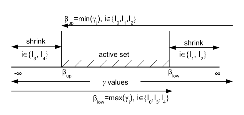
Shrinking is a mechanism to expedite the convergence of SVM training phase by eliminating the samples, which would not contribute to the hyperplane [17, 6]. With $I_{1},I_{2},I_{3}$ and $I_{4}$ defined as in (7), samples may be eliminated if they satisfy the following decision rule:

$$\begin{split}i\in\{I_{3}\cup I_{4}\}\quad and\quad\gamma_{i}<\beta_{up}\\ or\\ i\in\{I_{1}\cup I_{2}\}\quad and\quad\gamma_{i}>\beta_{low}\end{split}$$ (10)

This heuristic is explained in the Figure 1. The eliminated samples belong to one of the two classes: $a)$ ones that have $\alpha=0$ and $b)$ those with $\alpha=C$.

2.3 Programming Models

This paper uses two programming models - MPI [15, 13] and Global Arrays [19] for designing scalable SMO on distributed systems. Due to space limitations, we provide a brief background of Global Arrays and suggest other literature for MPI [15, 13].

2.3.1 Global Arrays

The Global Arrays programming model provides abstractions for distributed arrays, load/store semantics for local partition of the distributed arrays, and one-sided communication to the remote partitions. Global Arrays leverages the communication primitives provided by Communication Runtime for Exascale (ComEx) [27]. Global Arrays programming model has been used for designing many scalable applications in domains such as chemistry [25] and sub-surface modeling [23]. The Global Arrays infrastructure is useful in storing the entire dataset in a compressed row format. The easy access to local and remote portions of distributed arrays facilitates a design of algorithms which would need asynchronous read/write access to the arrays. Global Arrays uses ComEx network communication layer for one-sided communication.

3 Solution Space

Table 1: Representative notations used and their explanation

Name	Symbol
# of Processors	$p$
# of Training Points	$\mathcal{N}$
Class label	$y_{k}$
Lagrange multiplier	$\alpha_{k}$
Set of Support Vectors	$\zeta$
Working set	$\pi$
$\delta L_{D}/\delta\alpha_{k}$, $\gamma_{k}*y_{k}$ (5)	$\nabla_{k}$
Hyperplane threshold	$\beta$
Sample in CSR form	$\breve{x}$
Indices set $I_{0-4}$ in (7)	$\varsigma$
User-Specified Tolerance	$\epsilon$
Avg $\langle,.~{},\rangle$ time	$\lambda$
Row-Pointer Array	$\psi$
Average sample length $\left|\bm{x_{k}}\right|$	$m$
Network Latency	$l$
Network Bandwidth	$\frac{1}{G}$

This section begins with a presentation of various steps of the sequential SVM training algorithm 1, which is followed by a discussion of the data structures organization using the parallel programming models. Section 3.2 introduces the parallel training algorithm of the Original algorithm, and presents its time-space complexity. This is a followed by a discussion and analysis of multiple parallel shrinking algorithms 3.4

Input: $\mathcal{C}$, $\mathcal{\sigma}$, $\mathcal{X}\in\Re^{\mathcal{N}\times d}$, $y_{i}\in\{+1,-1\},i=1,2,\ldots\mathcal{N}$

Data: $\bm{\alpha}\in\Re^{\mathcal{N}\times 1}$

Result: $\zeta$

1 Initialize $\gamma_{i}=-y_{i},\alpha_{i}=0,\forall i$;

2 $i_{low}=\{j\mid y_{j}=1,j\in\{1,2,\ldots\mathcal{N}\}\}$;

3 $i_{up}=\{k\mid y_{k}=-1,k\in\{1,2,\ldots\mathcal{N}\}\}$ ;

4 repeat

5       Update $\alpha_{i_{low}}$ and $\alpha_{i_{up}}$ using (11);

6       Assign $i_{low}$ and $i_{up}$ to one of $\varsigma$ using (7);

7       $\forall i$, Update $\gamma_{i}$ using (6);

8       Calculate new $\beta_{low}$ and $\beta_{up}$ using (8);

9      

10until (9) succeeds;

Algorithm 1 Improved SMO - Modification 2 [18]

(a)

(b)

(c)

Figure 1: (1): Shrunk ids when (9) is not satisfied (non-optimality). Refer to (10) for the shrinking criterion. (1): Memory Space Conservation with CSR (1): $\breve{x}$: An extended sample prototype in CSR representation. Refer to Table 1 for the meaning of the symbols.

3.1 Preliminaries

Algorithm 1 shows the key steps of our sequential SVM algorithm. This is used as a basis for designing parallel SVM algorithms, with (Algorithms 5 and its variant) and without (Algorithm 3) shrinking. Using Table 1 as reference, at each iteration, $\forall i$, $\alpha_{i}$ is calculated based on (11). In most cases, the objective function is positive definite ($\rho<0$) 12, which is used as the basis for update. An approach proposed by Platt et al. [20] can be used for the update equations, when $\rho>0$.

$$\begin{split}\alpha_{i_{low}}^{new}=\alpha_{i_{low}}-y_{i_{low}}*(\gamma_{i_{up}}-\gamma_{i_{low}})/\rho\\ \alpha_{i_{up}}^{new}=\alpha_{i_{up}}+y_{i_{low}}*y_{i_{up}}*(\alpha_{i_{low}}-\alpha_{i_{low}}^{new})\end{split}$$ (11)

where

$$\begin{split}\rho=2*\Phi({\mathbf{x}}_{i_{low}})\cdot\Phi({\mathbf{x}}_{i_{up}})\\ -\Phi({\mathbf{x}}_{i_{up}})\cdot\Phi({\mathbf{x}}_{i_{up}})-\Phi({\mathbf{x}}_{i_{low}})\cdot\Phi({\mathbf{x}}_{i_{low}})\end{split}$$ (12)

Once (9) is satisfied, $\beta$ in (4) is calculated as:

$$\beta=\left\{\begin{array}[]{ll}\sum_{i\in I_{0}}\gamma_{i}/\left|I_{0}\right|&\textrm{if $\left|I_{0}\right|\neq 0$ }\\ (\beta_{low}+\beta_{up})/2&\textrm{otherwise}\end{array}\right.$$

3.1.1 Distributed Data Structures

There are several data structures required by algorithms 3 and 5 , which need to be distributed across different compute nodes. These data structures include the $\mathcal{X}$ for the input dataset, $y$ for the sample label, $\bm{\alpha}$ for the Lagrange multipliers, $\gamma$ and $\varsigma$. As presented earlier, the computation can be re-formulated to using a series of kernel calculations. The individual kernel calculations may be stored in a kernel cache, which itself can be distributed among different processes.

However, there are several reasons for avoiding kernel cache for large scale systems. The space complexity of complete kernel cache is $\Theta(\mathcal{N}^{2})$, which is prohibitive for large inputs - a primary target of this paper. At the same time, the temporal/spatial reuse of individual rows of kernel cache is low as the $i_{up}$ and $i_{low}$ typically do not exhibit a temporal/spatial pattern. As the architectural trends exhibit, the available memory per computation unit (such as a core in a multi-core unit) is decreasing rapidly, and it is expected that simple compute units such as Intel Xeon Phi would be commonplace [2], while Graphics Processors are already ubiquitous. At the same time, these compute units provide hardware support for wide-vector instructions, such as fused multiply-add. As a result, the cost of recomputation is expected to be much lower than either caching the complete kernel matrix or conducting off-chip/off-node data movement to get the individual rows of kernel matrix distributed across multiple nodes. Hence, the proposed approaches in this paper avoid the kernel cache altogether.

3.1.2 Data Structure Organization

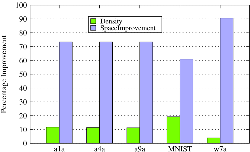
The organization of distributed data structures plays a critical role in reducing time and space complexity of algorithm 1. Most datasets are sparse in nature, with several datasets having less than 20% density. Figure 1 shows the percentage of memory space conserved when using a compressed sparse row (CSR) [11] representation. As shown in Figure 1, co-locating the algorithmic related data structures and making the column indices as part of representation makes little change in the density and the reduction in space complexity outweighs the additional bookkeeping for the boundaries of various samples.

The core steps of computation requires several kernel calculations and frequent access to the data structures such as the $y$, $\bm{\alpha}$, and $\gamma$. Among these, $y$ is a read-only data structure, while other data structures are read-write. The organization of these data structures with $\mathcal{X}$ has a significant potential of improving the cache-hit rate of the system, by leveraging the spatial locality. Although a few of these data structures are read-write, the write-back nature of the caches on modern systems make them a better design choice in comparison to the individual data structures distributed across multiple processes in the job. An additional advantage of co-location of these data structures with $\mathcal{X}$ is that load balancing among processes is feasible which requires contiguous data movement of samples, instead of several individual data structures.

For the proposed approaches, CSR is implemented using Global Arrays [19] programming model. Global Arrays provides semantics for collective creation of a compressed row, facilitating productive use of PGAS models for algorithms 3 and 5. GA provides Remote Memory Access semantics for traditional Ethernet based interconnects and Remote Direct Memory Semantics (RDMA), making it effective for distributed systems such as based on Cloud and tightly-connected supercomputers.

Input: Samples $\breve{x}$ and $\breve{y}$, len($\breve{x}$), len($\breve{y}$), where len represents the number of cells in the representation

Output: $\langle\breve{x},\breve{y}\rangle$, the inner product of $\breve{x}$ and $\breve{y}$

1 /* shift past the padded data */;

2$\grave{x}\leftarrow\breve{x}+4$, $\grave{y}\leftarrow\breve{y}+4$;

3 $s1\leftarrow 0$, $s2\leftarrow 0$, $dp\leftarrow 0$;

4 while $s1<len(\grave{x})-4~{}\&~{}s2<len(\grave{y})-4$ do

5       if $|\grave{x}[s1]-\grave{y}[s2]|<0$ then

6             $dp\leftarrow dp+\grave{x}[s1+1]*\grave{y}[s2+1]$;

7             $s1\leftarrow s1+2$;

8             $s2\leftarrow s2+2$;

9            

10       else if $\grave{x}[s1]<\grave{y}[s2]$ then

11             $s1\leftarrow s1+2$;

12            

13       else

14             $s2\leftarrow s2+2$;

15            

16      

17 return $\langle\breve{x},\breve{y}\rangle$;

Algorithm 2 Inner Product using CSR format

Algorithm 2 shows the pseudocode for the inner product calculation - the most frequently executed portion in our implementations. While the CSR representation is not conducive for using hardware based vector instructions, we leave the use of such vector units as a future work. The primary objective in this paper is to minimize the space complexity by using CSR representation not used by other papers such as [5]. The inner product is used as a constituent value in $\gamma$ (line 3 in algorithm 3) calculation by using a simple linear algebra trick.

Data: $p$: # processors, $P_{q}$: $q$-th processor, $0\leq q<p$,

$i\in\left[\,q*|\mathcal{X}|/p,~{}(q+1)*|\mathcal{X}|/p\,\right)$

Input: $\mathcal{C}$, $\mathcal{\sigma}$, $\hat{\mathcal{X}}\in\Re^{\frac{\mathcal{N}}{p}\times d}$, $y_{i}\in\{+1,-1\},\forall i$,

$\bm{\alpha}\in\Re^{\frac{\mathcal{N}}{p}\times 1}$

Result: $\zeta$

1 Initialize $\gamma_{i}=-y_{i},\alpha_{i}=0,\forall i$, $i_{low},i_{up}$

2 repeat

3       // MPI Broadcast Operation

4       Receive $\bm{x}_{i_{low}}$, $\bm{x}_{i_{up}}$ from proc$\#0$

5       Update $\alpha_{i_{low}}$ and $\alpha_{i_{up}}$ using (11)

6       Constrain ${\alpha}s$ as per (2)

7       for $\forall$i do

8             $li\leftarrow\psi_{i}$

9             $hi\leftarrow\psi_{i+1}-1$

10             $\breve{x}\leftarrow\textnormal{{GAget}}(li,hi)$

11             /* $\breve{x}[2]:=Gradient$. Refer to Figure 1 */

12             Update $\breve{x}[2]$ using (6)

13             if $i==i_{up}~{}or~{}i==i_{low}$ then

14                   $\breve{x}[0]\leftarrow\alpha_{i_{low}}~{}or~{}\alpha_{i_{up}}$

15                   Update $\varsigma$ using (7)

16                   // global copy update

17                  

18             $\textnormal{{GAput}}(\breve{x}[0:2])$

19              /* first 3 cells */

20            

21       $\beta_{up,local}\leftarrow min(\beta_{up_{i}})$

22       $\beta_{low,local}\leftarrow max(\beta_{low_{i}})$

23       // Using MPI Allreduction

24       $\beta_{up}$, $\beta_{low}\leftarrow~{}GlobalMinMax(\beta_{up,local},\beta_{low,local},p)$

25      

26until no KKT violators

Algorithm 3 Algorithm 1 parallel version; $q$-th CPU perspective.

1

2for $\forall i\in\pi_{q}$ do

3       $li\leftarrow\psi[i]$,$hi\leftarrow\psi[i+1]-1$

4       $\breve{x}\leftarrow\textnormal{{GAget}}(li,hi)$

5       if $i==i_{up}~{}or~{}i_{low}$ then

6             update $\breve{x}[0],~{}\breve{x}[1]$

7              /* $\alpha,\varsigma$ */

8            

9       update $\breve{x}[2]$

10        /* $\gamma$ */

11       $\textnormal{{GAput}}(\breve{x}[0:2])$

12       if $\neg shrinkitercounter$ then

13             apply (10) to $\breve{x}$

14             update $\pi_{q}$

15            

16      

17 if $\neg shrinkitercounter$ then

18       $shrinkitercounter\leftarrow MPI\_Allreduce(\left|\pi_{q}\right|)$

19      

20else

21       $shrinkitercounter{-}{-}$

22      

23 update global $\beta$ values

24

Algorithm 4 Parallel update of data structures following shrinking, $q-$th CPU perspective.

Data: $p$: # processors, $P_{q}$: $q$-th processor, $0\leq q<p$, $\pi$

Input: $\mathcal{C}$, $\mathcal{\sigma}$, $\hat{\mathcal{X}}\in\Re^{\frac{\mathcal{N}}{p}\times d}$, $y_{i}\in\{+1,-1\},\forall i$,

$\bm{\alpha}\in\Re^{\frac{\mathcal{N}}{p}\times 1}$

Result: $\zeta$

1 $i\in\left[\,startindex,~{}endindex\,\right)$, where $startindex\leftarrow q*|\mathcal{X}|/p$, $endindex\leftarrow(q+1)*|\mathcal{X}|/p$

2 Initialize $\gamma_{i}\leftarrow-y_{i},\alpha_{i}\leftarrow 0,\forall i$, $i_{low},i_{up}$

3 $\pi_{q}$[$0\ldots(endindex-startindex)]\leftarrow startindex\text{--}endindex$

4 while $1$ do

5       $outloop\leftarrow false$, $tolflag\leftarrow false$

6       if $shrink$ then

7             if $\beta_{up}<\beta_{low}-20\cdot\epsilon$ then

8                  

9             repeat

10                   Receive $\bm{x}_{i_{low}}$, $\bm{x}_{i_{up}}$ from proc$\#0$

11                   Update $\alpha_{i_{low}}$ and $\alpha_{i_{up}}$ using (11)

12                   Constrain ${\alpha}s$ to satisfy (2)

13                   Perform Algorithm 4

14                  

15            until failed

16            else

17                   $tolflag\leftarrow true$

18                  

19            

20      else  /* shrinking done once */

21             if $\beta_{up}<\beta_{low}-2\cdot\epsilon$ then

22                  

23             repeat

24                   Receive $\bm{x}_{i_{low}}$, $\bm{x}_{i_{up}}$ from proc$\#0$

25                   Update $\alpha_{i_{low}}$ and $\alpha_{i_{up}}$ using (11)

26                   Clip ${\alpha}s$ to the box constraint (2)

27                   Call Algorithm 4

28                  

29            until failed

30            else

31                   $tolflag\leftarrow true$

32                  

33            

34      if $\textnormal{{shrink}}~{}\&\left(\,outloop\|tolflag\,\right)$ then

35             gradientreconstruct ()

36              /* Algorithm 6 */

37             if $\beta_{up}<\beta_{low}-2\cdot\epsilon$ then

38                   $shrink\leftarrow 0$

39                   $shrinkitercounter\leftarrow\textnormal{{min\_shrink\_counter}}$

40                   Reset $\pi_{q}$

41                  

42             else

43                   break

44                    /* optimality reached */

45                  

46            

47       else

48             if $outloop\|tolflag$ then

49                   break

50                  

51            

52      

Algorithm 5 Parallel Shrinking with single call to Algorithm 6. $q$-th CPU perspective.

3.2 Parallel SVM training Algorithms

This section lays out the parallel algorithms - with shrinking 5 and without shrinking 3. It also presents the reasoning behind shrinking and the conditions which must be true at the point of shrinking.

3.2.1 Parallel algorithm

Algorithm 3 is a parallel no-shrinking variant of the sequential algorithm 1. This algorithm is also referred as Original in various sections of this paper. There are several steps in this algorithm. Each process receives $\bm{x}_{low},\bm{x}_{up}$ from a default process using the MPI broadcast primitive, which is a scalable logarithmic operation in the number of processes. Each process independently calculates the new $\bm{\alpha}$ corresponding to $i_{up}$ and $i_{low}$. This results in a time complexity of $O(l+m\cdot G)\cdot log(p)$ for network communication and three kernel calculations $3\cdot\lambda$ (ignoring other integer based calculation).

The for-loop over all samples for a process is the predominantly expensive part of the calculation. Each iteration requires the calculation of the $gradient$, which involves several kernel calculations, the $\varsigma$ calculation and update of the global values of $\alpha_{up}$ or $\alpha_{low}$, if they are locally owned by the process. The GAput operation (line  3) updates only the indices, which were updated during the calculation, reducing the overall communication cost. The computation cost of this step is $\Theta(\lambda\cdot\frac{\left|\mathcal{X}\right|}{p})$. For a sufficiently large $\frac{\left|\mathcal{X}\right|}{p}$, the $\varsigma$ calculation and the communication cost to update the global copy of $\alpha$ can be ignored. The last step of the algorithm is to obtain the globally maximum and minimum of $\beta_{low}$, and $\beta_{up}$, respectively. This is designed using MPI Allreduction operation which has a time-complexity of $\Theta(l\cdot log(p))$ (The bandwidth term can be ignored, since this step involves a communication of only two scalars).

3.3 Shrinking Algorithms

Joachims et al. [17] and Lin et al. [6] have previously demonstrated the impact of adaptive elimination of samples - shrinking. This technique is a heuristic, since the sufficient conditions to identify the samples to be eliminated are unknown [17]. For the eliminated samples, the Lagrange multipliers are kept fixed and they are not considered during the working set selection and the check for optimality. This results in time-complexity reduction, since the gradient for eliminated samples is not computed. The primary intuition behind shrinking is that only a small subset of samples contributes towards hyperplane definition:

$$\begin{split}\mathcal{A}=\{\,k\mid\gamma_{k}<\beta_{low}~{}or~{}\gamma_{k}>\beta_{up},0<\alpha_{k}\,\}\\ \textrm{and}\\ \left|\mathcal{A}\right|\ll\left|\mathcal{X}\right|\end{split}$$ (13)

It is expected that when the optimization is at the early stage, some of the bound samples $(\alpha_{k}=0,~{}\alpha_{k}=C)$ stabilize [17].

$$\begin{split}\textrm{At non-optimality after sufficient iterations:}\\ \mathcal{\grave{A}}=\{\,k\mid\beta_{low}\geq\gamma_{k}\geq\beta_{up}\,\}\end{split}$$ (14)

where $\mathcal{\grave{A}}$ is the set of violators from where working set variables are chosen and one or more samples from the set $\mathcal{X}-\mathcal{\grave{A}}$ can be eliminated without changing the current solution. Specifically, (10) presents a variant of the condition proposed previously by Lin et al. for shrinking. The overhead of calculating which samples to shrink is expected to be $\Theta(1)$, since the computation only involves a few conditions.

However, there are several problems with this assumption. It is possible that samples with $\alpha\in\{0,C\}$ - which were previously eliminated - eventually stabilize to a value between $0$ and $C$. A premature elimination of these samples may result in the incorrect definition of hyperplane. A conservative approach to decide on the execution of this condition may not be beneficial, since much of the calculation would likely have completed. In essence, it is very difficult to predict the point at which to execute this condition. Lin et al. have proposed to use $min(|\grave{A}|,1000)$ iterations as the point to perform shrinking. However, there is no intuitive reasoning behind selecting a value to begin or executed shrinking. A discussion on spectrum of heuristics for shrinking is presented in the next section.

3.3.1 Shrinking Heuristics

The heuristics for shrinking considered in this paper are to address the concerns of early elimination of the samples, while still reducing the overall time for SVM convergence. In general, $\left|\zeta\right|$ $\ll$ $\left|\mathcal{X}\right|$. Using this intuition, we propose several heuristics for shrinking, which are based on the $\left|\mathcal{X}\right|$. An aggressive shrinking heuristic would use a $n\cdot\left|\mathcal{X}\right|$ as the iteration count for initial shrinking, where $n\ll 1$. A conservative shrinking heuristic could use a larger value of $n$. This method is referred to as numsamples based approach in Table 3. An alternative technique is to use initial shrinking iteration counter to be a random value, similar to the approach proposed by Lin et al. For each of these heuristics, the subsequent calculation of shrinking iteration is a minimum of $\left|\mathcal{X}\right|$ or $|\grave{A}|$ (depending on the algorithms) and the value of shrinking iteration calculated using the proposed heuristics. See section 4.3 for further discussion on this topic.

3.4 Gradient Reconstruction

Gradient reconstruction is an important step in ensuring that the previously eliminated samples are not false positives and that they are on the correct side of the hyperplane in the final solution. Algorithm 6 shows the key steps involved in updating $\gamma$ values during the gradient reconstruction step of the algorithm 5. The algorithm 5 corresponds to shrinking with single gradient-reconstruction. An algorithm, which corresponds to multiple gradient reconstruction (Refer to Table 3) can be derived from this. However, due to lack of space, it is not presented explicitly.

Algorithm 6 finds the $\gamma$ values of all the eliminated samples from the previous gradient reconstruction. To achieve this, it needs $\mathcal{X}-\grave{A}$, which results in the communication of samples owned by each process. The time complexity of this step is $l+|\mathcal{X}-\grave{A}|\cdot G$ $\approx$ $|\mathcal{X}-\grave{A}|\cdot G$. The communication cost may be non-negligible for distributed systems, hence it is necessary to consider heuristics which limit the execution of gradient synchronization step. Also evident from the loop structure is the fact that the outer loop considers all eliminated samples of the $q$-th CPU and updates their gradient values. This is a computationally expensive operation since line 6 involves kernel calculations ((5) from section 2.2), so this algorithm is called only when global violators are within a specific threshold (e.g., lines 5 and 5 in Algorithm 5). Since $\gamma$ plays an important role in both the $\alpha$ updates (11) and working set selection (Section 2.2.2), we maintain it for all the active samples throughout the program execution.

Considering a less-noisy dataset, $\left|\zeta\right|\ll\mathcal{N}$ and on an average, $\pi_{q}=\frac{\zeta}{p}$. Then, $\left|\omega\cap\zeta\right|$ is small if not $0$ and the computational time complexity expected for $q$-th CPU for Algorithm 6 is $\left|\omega_{q}\right|\cdot\left|\zeta\right|\cdot\lambda=\left|\frac{\mathcal{X}-\zeta}{p}\right|\cdot\left|\zeta\right|\cdot\lambda$. The tradeoff between $\left|\omega\right|$ and $\left|\zeta\right|$ is clear making this essential algorithm a bottleneck in achieving the overall speedup in convergence. As a result, we have considered single and multi heuristics for $\gamma$-reconstruction as shown in Figure 3.

Data: $p$: # processors, $P_{q}$: $q$-th processor, $0\leq q<p$, $\pi$

Input: $\mathcal{\sigma}$, $\hat{\mathcal{X}}\in\Re^{\frac{\mathcal{N}}{p}\times d}$, $y_{i}\in\{+1,-1\},\forall i$

1 // Gather eliminated samples of this process

2 $li\leftarrow\psi_{0}$

3 $hi\leftarrow\psi_{|\mathcal{X}|}$

4 GAget($li,hi$)

5 $\omega_{q}=\hat{\mathcal{X}}-\pi_{q}$

6 for $\forall\breve{a}\in\omega_{q}$ do

7       $my\gamma\leftarrow 0$

8       for $\{\,\forall\breve{b}\in\mathcal{X}\mid\breve{b}[0]>0\,\}$ do

9             $my\gamma~{}+=\breve{b}[0]*\breve{b}[3]*(\Phi({\mathbf{a}})\cdot\Phi({\mathbf{b}}))$

10            

11       $\breve{a}[2]=my\gamma-\breve{a}[3]$

12       GAPut($\breve{a}[2]$)

13      

14 // MPI All reduction

15 Update global $\beta_{low}$ and $\beta_{up}$

Algorithm 6 Gradient Reconstruction; $q$-th CPU perspective.

4 Empirical Evaluation

This section provides an empirical evaluation of the proposed approaches in the previous section. The empirical evaluation is conducted across multiple dimensions: datasets, number of processes, shrinking/no-shrinking, heuristics for selection of shrinking steps. The performance evaluation uses up to 512 processes (32 compute nodes), and several datasets use between 1 and 32 compute nodes. As a result, the proposed approaches can be used on multi-core machines such as a desktop, supercomputers or cloud computing systems. For each dataset, we compare our results with LIBSVM [6], version 3.17, with shrinking enabled.

The upcoming sections provide a brief description of the datasets, experimental testbed and followed by empirical results. Due to accessibility limitations, the performance evaluation is conducted on a tightly connected supercomputer, although the generality of our proposed solution makes it effective for cloud computing systems as well.

Table 2: Dataset Characteristics and hyperparameter settings

Name	Training Set Size	Testing Set Size	C	$\sigma^{2}$
MNIST	60000	10000	10	25
Adult-7 (a7a)	16100	16461	32	64
Adult-9 (a9a)	32561	16281	32	64
USPS	7291	2007	8	16
Mushrooms	8124	N/A	8	64
Web (w7a)	24692	25057	32	64
IJCNN	49990	91701	0.5	1

4.1 Datasets

Table 2 provides a description of the datasets used for performance evaluation in this paper. The MNIST dataset represents images of handwritten digits. The dimensions are formed by flattening the 28x28 pixel box into one-dimensional array of floating point values between 0 and 1, with 0 representing black and 1 white. The 10-class dataset is converted into a two-class one by representing even digits as class -1 and odd digits as +1. The sparse binary Adult dataset represents the collected census data for income prediction. Web dataset is used to categorize web pages based on their text [20]. USPS represents a collection of handwritten text recognition, collected by United States Postal Service. The mushrooms data set includes descriptions of hypothetical samples corresponding to 23 species of gilled mushrooms in the Agaricus and Lepiota Family. The IJCNN dataset represents the first problem of International Joint Conference on Neural Nets challenge 2001. Hyperparameter settings for the datasets have been selected after doing multi-fold cross-validation [6]. These are shown in Table 2. The hyperparameter $C$ is described in section 2.1 and $\sigma^{2}$ is the kernel width in the Gaussian kernel: $K({\mathbf{x}},{\mathbf{y}})=\exp(-\|{\mathbf{x}}-{\mathbf{y}}\|^{2}/2\sigma^{2})$. It is straightforward to use other kernels in this work.

4.2 Experimental Testbed

All our experiments were run on PNNL Institutional Computing (PIC) cluster . PIC Cluster consists of 692 dual-socket nodes with 16 cores per socket AMD Interlagos processors, running at 2.1 GHz with 64 GB of 1600 MHz memory per node (2 GB/socket). The nodes are connected using InfiniBand QDR interconnection network. The empirical evaluation consists of a mix of results on single node (multi-core) and multiple nodes (distributed system). While the performance evaluation is on a tightly-connected system, most modern Cloud providers provide programming models such as MPI and Global Arrays, hence this solution is deployable on them as well.

4.3 Heuristics: An overview

Table 3 provides a list of heuristics, which are used for evaluation on datasets presented in the previous section. Specific values to aggressive, conservative and average methods for shrinking are provided. To emulate the heuristics evaluated by Lin et al., we also compare several values of random sample elimination as suggested in the Table. Line $2$ in the table is to be interpreted as shrinking every 2 iterations(aggressive), with a single call to gradient reconstruction. Optimization proceeds without shrinking after this call. Similarly, line $13$ can be read as shrinking whenever the number of iterations reach half the number of samples (conservative) with multiple calls to $\gamma$ reconstruction as deemed fit and optimization proceeds with shrinking throughout until convergence.

Table 3: Heuristics. Description and classification. $\star$: Aggressive shrinking class, $\bullet$: Conservative, $\diamond$: Average

#	Shrinking Type	$\gamma$-Recon.	Name	Class
$1)$	None	N/A	Original	N/A
$2)$	random: 2	Single	Single2	$\star$
$3)$	random: 500	Single	Single500	$\star$
$4)$	random: 1000	Single	Single1000	$\diamond$
$5)$	numsamples: 5%	Single	Single5pc	$\star$
$6)$	numsamples: 10%	Single	Single10pc	$\diamond$
$7)$	numsamples: 50%	Single	Single50pc	$\bullet$
$8)$	random: 2	Multi	Multi2	$\star$
$9)$	random: 500	Multi	Multi500	$\star$
$10)$	random: 1000	Multi	Multi1000	$\diamond$
$11)$	numsamples: 5%	Multi	Multi5pc	$\star$
$12)$	numsamples: 10%	Multi	Multi10pc	$\diamond$
$13)$	numsamples: 50%	Multi	Multi50pc	$\bullet$
$14)$	Default	Default	LIBSVM	N/A

Figure 2: Adult (a7a) Dataset Performance

Figure 3: Adult (a9a) Dataset Performance

Figure 4: MNIST Dataset Performance

Figure 5: USPS Dataset Performance

Figure 6: w7a Dataset Performance

Figure 7: Mushroom Dataset Performance

Figure 8: IJCNN Dataset Performance.

Name	Test Acc. - Ours(%)	Test Acc.-LIBSVM(%)	Speedup(Original)	Speedup (LIBSVM)
Adult-7	83.75	84.81	1.6x	3.5x
Adult-9	84.68	83.12	1.4x	3.7x
USPS	97.6	97.75	1.7x	5x
Web	98.86	98.8	1.6x	3.3x
MNIST	96.63	98.62	1.2x	26x
Mushrooms	N/A	N/A	3x	8.2x
IJCNN	90.3	96.58	N/A	9x (Orig)

Figure 9: Summary of Results (Testing Accuracy and Relative Speedups between our best performing heuristic with the Original Implementation 3 and LIBSVM)

4.4 Results and Analysis

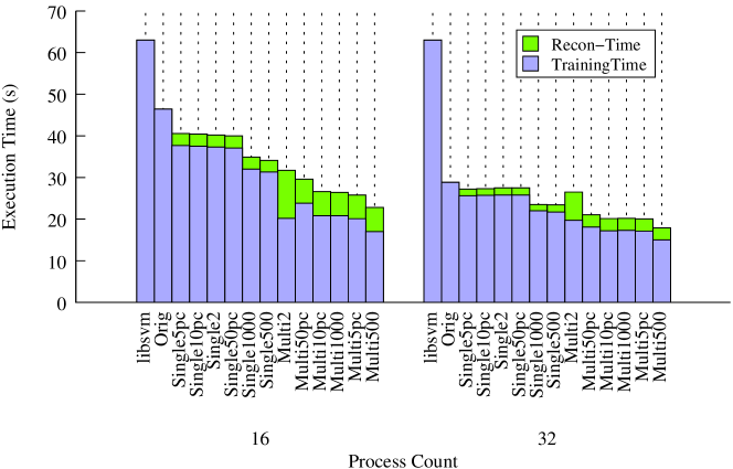
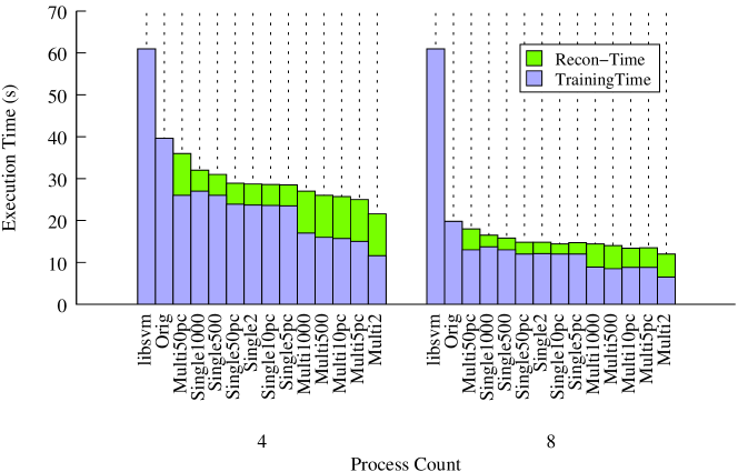
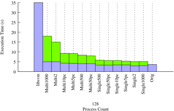
Figures 3 and 3 show the results for Adult-7 and Adult-9 datasets, respectively. A speedup of $\approx$ 2x is observed on Adult-7 dataset using the Multi500 and Multi5pc heuristics in comparison to Original algorithm, and 3-3.5x in comparison to LIBSVM. Among all the approaches, Multi2 has the highest time in $\gamma$ Reconstruction (referred as Recon-Time in the figures), largely because it eliminates samples prematurely, while other heuristics allow the $\alpha$ values to stabilize before elimination. It is worthwhile noting that each of the Multi* heuristics are better than Single shrinking for these datasets. For each of the adult datasets, $\left|\zeta\right|$ $\ll$ $X$, which is a suitable condition for shrinking. Since the proposed heuristics are precise, the accuracy and time for classification for each of these datasets is similar, and only a representative information is shown in Table 9. It is also worthwhile noting that the implementation of the original algorithm is near optimal, as it scales well with increasing number of processes.

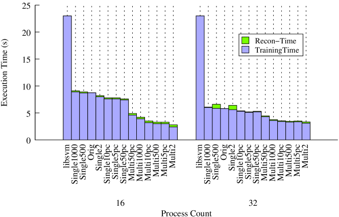
The results for USPS dataset, as shown in Figure 5 show the efficacy of highly aggressive Multi2 heuristic, with Multi5pc being the second best. These results validate our premise, that $\left|\zeta\right|$ is typically small, and a multiple 5% heuristic such as Multi5pc can provide significant elimination of computation for SVM, resulting in faster convergence. As discussed previously, the first $\gamma$ reconstruction is executed at $20\cdot\epsilon$, while others are executed $2\cdot\epsilon$. However, with Multi* heuristics, the number of times the gradient is reconstructed at the terminating condition can be predicted apriori. As shown in the USPS results, each of the Multi* shrinking heuristics, although spend significantly more time in gradient reconstruction( 6), still reduce the overall execution time. For USPS dataset, an overall speedup of $\approx$ 1.7x is observed in comparison to Original implementation, and 5x in comparison to LIBSVM.

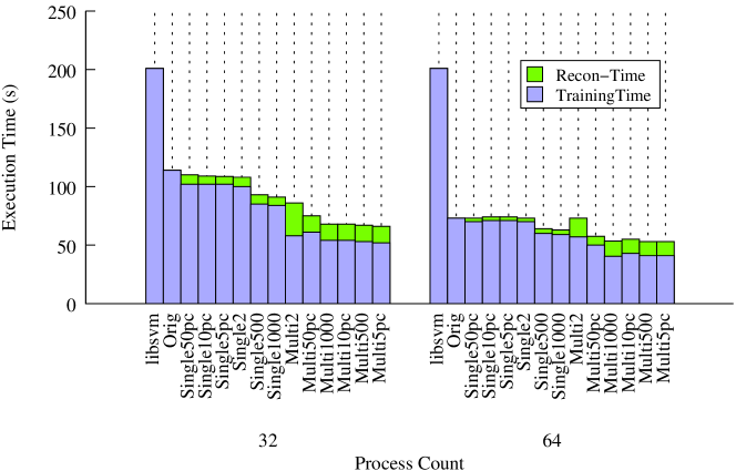
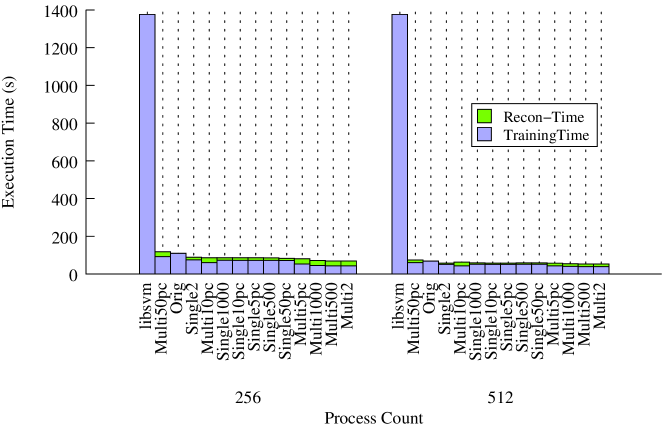
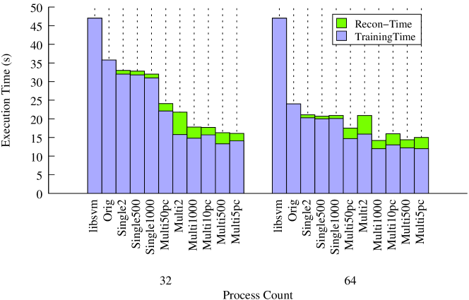
Figure 5 shows the performance of various approaches on MNIST dataset using 256 and 512 processes - equivalent of 16 and 32 compute nodes. There are several take away messages - the original implementation scales well providing about 1.2x speedup or $\approx$ 90% efficiency. Several Multi* heuristics perform very well, with little difference in execution time among them. For 256 processes, a speedup of more than 1.3x is achieved using Multi1000 approach in comparison to the original approach and 26x over LIBSVM. The fact that more time is spent in $\gamma$ reconstruction is outweighed by the overall reduction in the training time. Similar trends are observed with the w7a dataset shown in Figure 7, where 2.3x speedup is observed on 32 processes and 1.6x speedup is observed on 64 processes, with up to 3.3x speedup in comparison to LIBSVM.

Figure 7 shows the performance on the Mushrooms dataset. In comparison to other datasets Mushrooms dataset requires significantly more relative time for training due to the higher values of $C$ and $\sigma^{2}$. As a result, the reconstruction time is relatively small. $\frac{276}{8124}$ are support vectors, which is less than 5% of the overall training set. Here as well, Multi5pc provides near-optimal performance resulting in $\approx$ 3x speedup, while Multi2 is slightly better than that. Again, it is fair to conclude that Multi5pc is a good heuristic in extracting the benefits of shrinking. Up to 8.2x improvement is observed in comparison to LIBSVM.

Figure 9 shows the performance of IJCNN data set. We have used this as an example to indicate that shrinking is not beneficial for all datasets and different setting of hyperparameters. For several datasets, we have observed that higher values of hyperparameters results in faster elimination of samples, potentially providing benefits of shrinking. This opens up a new avenue for research where shrinking is integrated in the cross-validation step to get parameters suitable for both shrinking and better generalization. As shown in the figure, the original implementation is the best, while each of the other approaches result in significant degradation due to shrinking. However, in comparison to LIBSVM, a speedup of up to 9x is observed with the Original implementation.

5 Related Work

We discuss SVM training algorithms in literature under two major branches of study: $1)$ the sample selection methods and $2)$ parallel algorithms.

5.1 Sample Selection

Multiple researchers have proposed algorithms for selection of samples, which can be be used for faster convergence. Active set methods solve the dual optimization problem by considering a part of the dataset in a given iteration until global convergence [20, 17, 18, 4, 5, 14, 8]. The primary approach is to decompose large Quadratic Programming tasks into small ones. Other approaches include the reformulation of the optimization problem, which does not require the decomposition [31]. The seminal SMO [20] and SVM^light [17] are active set sequential methods and SVM-GPU [5], and PSMO [4] are examples of parallel decomposition methods whereas Woodsend et al.[29] is an example of a parallel non-decomposition solution. A primary problem with the working set methods is the inability to address noisy, non-separable datasets [30]. However, the simplicity, ease of implementation and strong convergence properties make them an attractive choice for solving large-scale classification problems. Other researchers have considered different values ($>2$) of the working set [8, 17].

5.2 Parallel Algorithms

With the advent of multi-core systems and cluster computing, several parallel and distributed algorithms have been proposed in literature. This section provides a brief overview of these algorithms.

Architecture specific solutions such as GPUs [5, 8] have been proposed, and other approaches require a special cluster setup [14]. Graf et al. have proposed Cascade SVM [14], which provides a parallel solution to the dual optimization problem. The primary approach is to divide the original problem in completely independent sub-problems, and recursively combine the independent solutions to obtain the final set of support vectors. However, this approach suffers from load imbalance, since many processes may finish their individual sub-problem before others. As a result, this approach does not scale well for very large scale processes - a primary target of our approach.

The advent of SIMD architectures such as GPUs has resulted in research conducted for Support Vector Machines on GPUs [5]. Under this approach, a thread is created for each data point in the training set and the MapReduce paradigm is used for compute-intensive steps. The primary approach proposed in this paper is suitable for large scale systems, and not restricted to GPUs.

Several researchers have proposed alternative mechanisms for solving QP problems. An example of variable projection method is proposed by Zanghirati and Zanni [32]. They use an iterative solver for QP problems leveraging the decomposition strategy of SVM^light [17]. Chang et al.  [7] have also considered more than 2 active set size and solves the problem using Incomplete Cholesky Factorization and Interior Point method (IPM). Woodsend et al. [29] have proposed parallelization of linear SVM using IPM and a combination of MPI and OpenMP. However, their approach is not an active set method, as it does not decompose a large problem into smaller ones. There are approaches like [22] that solve the primal problem for linear SVMs for very large problems, but the primary objective of this paper is to scale the most popular 2-working set based methods due to their ubiquity.

As evident from the literature study above, none of the previously proposed approaches use adaptive elimination of samples on large scale systems, which has a significant potential in reducing the execution time for several datasets.

6 Conclusions and Future Work

This paper has endeavored to address the limitations of previously proposed approaches and provided a novel parallel Support Vector Machine algorithm with adaptive shrinking. It explored various design aspects of the algorithm and the associated implementation, such as space complexity reduction by using sparse data structures, intuitive heuristics for adaptive shrinking of samples, and adaptive reconstitution of the data structures. We have used state-of-the-art programming models such as Message Passing Interface (MPI) [15] and Global Arrays [26] for the design of communication and data storage in the implementations. Empirical evaluation has demonstrated the efficacy of our proposed algorithm and the heuristics.

The future work involves shrinking with second order heuristics for working set selection, with deeper evaluation of heuristics and, considering other algorithms and working set sizes for faster elimination of samples. It will also be interesting to study shrinking under different architectures like GPUs. Though the proposed approach does complete elimination of kernel cache, it is possible to use deep memory hierarchy for keeping active portions of the kernel cache. The future work would also involve optimizations on upcoming architectures such as Intel MIC architecture, and AMD Fusion APU architecture.

References

- [1] P. Balaprakash, Y. Alexeev, S. A. Mickelson, S. Leyffer, R. L. Jacob, and A. P. Craig. Machine learning based load-balancing for the cesm climate modeling package. 2013.
- [2] K. Bergman, S. Borkar, D. Campbell, W. Carlson, W. Dally, M. Denneau, P. Franzon, W. Harrod, J. Hiller, S. Karp, S. Keckler, D. Klein, R. Lucas, M. Richards, A. Scarpelli, S. Scott, A. Snavely, T. Sterling, R. S. Williams, K. Yelick, K. Bergman, S. Borkar, D. Campbell, W. Carlson, W. Dally, M. Denneau, P. Franzon, W. Harrod, J. Hiller, S. Keckler, D. Klein, P. Kogge, R. S. Williams, and K. Yelick. Exascale computing study: Technology challenges in achieving exascale systems peter kogge, editor and study lead, 2008.
- [3] C. J. C. Burges. A tutorial on support vector machines for pattern recognition. Data Min. Knowl. Discov., 2:121–167, June 1998.
- [4] L. J. Cao, S. S. Keerthi, C.-J. Ong, J. Q. Zhang, U. Periyathamby, X. J. Fu, and H. P. Lee. Parallel sequential minimal optimization for the training of support vector machines. IEEE Transactions on Neural Networks, 17(4):1039–1049, July 2006.
- [5] B. Catanzaro, N. Sundaram, and K. Keutzer. Fast support vector machine training and classification on graphics processors. In Proceedings of the 25th international conference on Machine Learning, ICML ’08, pages 104–111. ACM, 2008.
- [6] C.-C. Chang and C.-J. Lin. LIBSVM: A library for support vector machines. ACM Transactions on Intelligent Systems and Technology, 2:27:1–27:27, 2011. Software available at http://www.csie.ntu.edu.tw/~cjlin/libsvm.
- [7] E. Y. Chang, K. Zhu, H. Wang, H. Bai, J. Li, Z. Qiu, and H. Cui. Psvm: Parallelizing support vector machines on distributed computers. In NIPS, 2007. Software available at http://code.google.com/p/psvm.
- [8] A. Cotter, N. Srebro, and J. Keshet. A GPU-tailored approach for training kernelized SVMs. In Proceedings of the 17th ACM SIGKDD international conference on knowledge discovery and data mining, KDD ’11, pages 805–813, 2011.
- [9] N. Cristianini and J. Shawe-Taylor. An introduction to support vector machines: and other kernel-based learning methods. Cambridge University Press, 2000.
- [10] DOE ASCAC Subcommittee. Synergistic Challenges in Data-Intensive Science and Exascale Computing, 2013.
- [11] J. Dongarra. Sparse matrix storage formats. In Z. Bai, J. Demmel, J. Dongarra, A. Ruhe, and H. van der Vorst, editors, Templates for the Solution of Algebraic Eigenvalue Problems: A Practical Guide. SIAM, Philadelphia, 2000.
- [12] R. Fletcher. Practical methods of optimization; (2nd ed.). Wiley-Interscience, New York, NY, USA, 1987.
- [13] A. Geist, W. Gropp, S. Huss-Lederman, A. Lumsdaine, E. L. Lusk, W. Saphir, T. Skjellum, and M. Snir. MPI-2: Extending the message-passing interface. In Euro-Par, Vol. I, pages 128–135, 1996.
- [14] H. P. Graf, E. Cosatto, L. Bottou, I. Durdanovic, and V. Vapnik. Parallel support vector machines: The cascade svm. In Advances in Neural Information Processing Systems, pages 521–528. MIT Press, 2005.
- [15] W. Gropp, E. Lusk, N. Doss, and A. Skjellum. A High-Performance, Portable Implementation of the MPI Message Passing Interface Standard. Parallel Computing, 22(6):789–828, 1996.
- [16] C.-J. Hsieh, K.-W. Chang, C.-J. Lin, S. S. Keerthi, and S. Sundararajan. A dual coordinate descent method for large-scale linear svm. In Proceedings of the 25th International Conference on Machine Learning, ICML ’08, pages 408–415, New York, NY, USA, 2008. ACM.
- [17] T. Joachims. Making large-scale support vector machine learning practical. In B. Schölkopf, C. J. C. Burges, and A. J. Smola, editors, Advances in kernel methods, pages 169–184. MIT Press, 1999.
- [18] S. S. Keerthi, S. K. Shevade, C. Bhattacharyya, and K.R.K.Murthy. Improvements to platt’s smo algorithm for svm classifier design. Neural Computation, 13(3):637–649, 2001.
- [19] J. Nieplocha, R. J. Harrison, and R. J. Littlefield. Global Arrays: A Nonuniform Memory Access Programming Model for High-Performance Computers. Journal of Supercomputing, 10(2):169–189, 1996.
- [20] J. C. Platt. Fast training of support vector machines using sequential minimal optimization. In Advances in kernel methods: support vector learning, pages 185–208, Cambridge, MA, USA, 1999. MIT Press.
- [21] Report from the DOE ASCR 2011 Workshop on Exascale Data Management, Analysis, and Visualization. Scientific Discovery at the Exascale, 2011.
- [22] S. Shalev-Shwartz, Y. Singer, and N. Srebro. Pegasos: Primal estimated sub-gradient solver for svm. In Proceedings of the 24th International Conference on Machine Learning, ICML ’07, pages 807–814, New York, NY, USA, 2007. ACM.
- [23] Subsurface Transport over Multiple Phases. STOMP. http://stomp.pnl.gov/.
- [24] A. L. Tarca, V. J. Carey, X.-w. Chen, R. Romero, and S. Drăghici. Machine learning and its applications to biology. PLoS Comput Biol, 3(6):e116, 06 2007.
- [25] M. Valiev, E. Bylaska, N. Govind, K. Kowalski, T. Straatsma, H. V. Dam, D. Wang, J. Nieplocha, E. Apra, T. Windus, and W. de Jong. Nwchem: A comprehensive and scalable open-source solution for large scale molecular simulations. Computer Physics Communications, 181(9):1477 – 1489, 2010.
- [26] A. Vishnu, J. Daily, and B. Palmer. Scalable PGAS Communication Subsystem on Cray Gemini Interconnect. Pune, India, 2012. HiPC.
- [27] A. Vishnu, D. J. Kerbyson, K. Barker, and H. J. J. V. Dam. Designing scalable pgas communication subsystems on blue gene/q. Boston, 2013. 3rd Workshop on Communication Architecture for Scalable Systems.
- [28] A. Vossen. Support vector machines in high-energy physics. 2008.
- [29] K. Woodsend and J. Gondzio. Hybrid mpi/openmp parallel linear support vector machine training. J. Mach. Learn. Res., 10:1937–1953, Dec. 2009.
- [30] E. Yom-tov. A parallel training algorithm for large scale support vector machines. Neural Information Processing Systems Workshop on Large Scale Kernel Machines, 2004.
- [31] L. Yuh-jye and O. L. Mangasarian. RSVM: Reduced support vector machines. Technical Report 00–07, Data Mining Institute, Computer Sciences Department, University of Wisconsin, 2001.
- [32] G. Zanghirati and L. Zanni. A parallel solver for large quadratic programs in training support vector machines. Parallel Computing, 29(4):535–551, 2003.