Predictions of a model of weak scale from dynamical breaking of scale invariance

Giulio Maria Pelaggi
Dipartimento di Fisica dell’Università di Pisa and INFN
   Pisa    Italy
g.pelaggi@for.unipi.it
Abstract

We consider a model where the weak and the Dark Matter scale arise at one loop from the Coleman-Weinberg mechanism, where the spontaneous symmetry breaking is driven by the Higgs and a new scalar boson. The latter is a doublet under the new gauge group SU(2)XsubscriptSU(2)𝑋\text{SU(2)}_{X} of the lagrangian. The new gauge vector is a good candidate to represent the Dark Matter particle. We perform a precise computation of the model predictions for the production cross section of the new scalar and for the direct-detection cross section of the DM particle, as a function of the only free parameter of the theory. The model can be tested directly in the next run of LHC and in the experiments LZ and XENON1T, because it provides particles in a slightly higher range of energies than the actual experimental limits.

1 Introduction

One year ago, the first LHC run ended. Its most important result is the discovery of a particle, with a mass of about 126 GeV, that is fully compatible with the Higgs boson of the Standard Model (SM) [1, 2]. This data confirms that the predictions on the SM spectrum were true, but the success of the SM hides another result: the complete absence of new physics.

Though the SM explains a wide range of physical phenomena, it has still some unsatisfactory aspects.

One of them is known with the name of “hierarchy problem” [3]. Why the dimensional parameters of the SM, that is the Higgs mass, has to get the value that we can measure experimentally? The SM doesn’t explain the link between the Higgs mass and other fundamental energy scales, e.g. the Planck mass. To describe our world, we need to “fine-tune” the parameters, that is, we have to set precisely their bare value to reproduce the experimental value.

A guideline for the physics beyond the SM may be naturalness [3]. Fundamentally we introduce some new physics, such that the divergent parts of the correction to the Higgs mass given by the SM are canceled by the new particles and interactions, while the remaining corrections are smaller than Mh2superscriptsubscript𝑀2M_{h}^{2}. In other words, naturalness suggests the existence of new physics at a certain scale ΛnatsubscriptΛnat\Lambda_{\text{nat}}. The corrections due to the SM are δMh2Λnat2similar-to𝛿superscriptsubscript𝑀2superscriptsubscriptΛnat2\delta M_{h}^{2}\sim\Lambda_{\text{nat}}^{2}, so if we want small corrections with respect to Mh2superscriptsubscript𝑀2M_{h}^{2}, the new physics has to be at low energies. Therefore, we hope that the new physics could explain the origin of the unpredicted values of the parameters of the Standard Model.

Looking at the data of the last period, i.e. the absence of these particles around the weak scale, the scale of the new physics had to move towards greater energy values. Maybe naturalness is a wrong way, but we think that some aspects of it can be recovered.

The model we will consider in this article is not UV complete, so the new physics added to the Standard Model doesn’t cancel automatically the divergences to the Higgs mass. The “finite naturalness” is a way to explain how to deal with these divergences. We think that the unknown physical cut-off behaves like in dimensional regularization computations: the divergent parts of the correction are unphysical, so we can neglect them. The reliability of finite naturalness for the SM has been studied in [4].

The fundamental idea is to start from a model with a lagrangian that doesn’t have any mass terms for scalar particles: the Coleman-Weinberg mechanism provides us a method to explain a non-zero value of the masses, also if the mass term is null, considering the radiative corrections of the theory. In fact, Coleman and Weinberg explain that the Spontaneous Symmetry Breaking (SSB) is not necessarily driven by a negative mass term for the scalar particle, but it can arise because of high-order processes involving virtual particles [5]. In fact, if we consider the one-loop effective potential of our model, new minima arise and SSB occurs.

In this way we get rid of the presence of dimensional parameters that make the lagrangian not scale invariant, and, following the idea of the finite naturalness, we don’t get quadratic divergences. Some models with this peculiarity has already been studied, for example in [6, 7, 8, 9, 10, 11, 12, 13, 14, 15, 16, 17, 18, 19].

The SM doesn’t provide a description of the Dark Matter. Today we can “see” it only through gravitational interactions. If we want to describe it as a particle, none of the particles we already know are good candidates.

The model that we are going to study has been proposed in [20, 22, 21]: the stability of the DM particle is not given by an ad hoc symmetry, but only because the gauge symmetry of the lagrangian and because of the particle content of the theory. The same happens in the SM, where the photon, the electron, the proton and the lightest neutrino are stable. In this model, the DM particle is a multiplet of vector particles. Following this idea, we want to introduce a new hidden sector of the lagrangian, that is connected to the SM only through a scalar quartic interaction with the Higgs boson (Higgs portal). For this purpose, we have to introduce a new scalar particle.

In the following sections, we compute more precisely if this model can be confirmed by the experimental data, maybe in the next phase of the work of LHC. We will analyze the general properties of the model in Section 2, in Section 3 we show all the computations done in the most general case, while in Section 4 we show the results and we discuss them.

2 The model

In this section we will briefly study the properties of this model. In particular we will explain why should we study the one-loop effective potential of the theory.

2.1 Lagrangian and particle content

We choose SU(2)XX{}_{\text{X}} as the new gauge group of the lagrangian, so the entire model is symmetrical under U(1)×Y{}_{\text{Y}}\timesSU(2)×L{}_{\text{L}}\timesSU(3)×c{}_{\text{c}}\timesSU(2)XX{}_{\text{X}}. The particle content is given by the SM particle content; plus we introduce doublet S𝑆S of the group SU(2)XX{}_{\text{X}}, that is a Lorentz scalar and a singlet under the SM symmetry group. We call Xμsubscript𝑋𝜇X_{\mu} the SU(2)XX{}_{\text{X}} vectors. These particles are, according to the model, the ones that constitute the Dark Matter. Xμsubscript𝑋𝜇X_{\mu} bosons can be described as Xμ=XμaTasubscript𝑋𝜇superscriptsubscript𝑋𝜇𝑎superscript𝑇𝑎X_{\mu}=X_{\mu}^{a}T^{a}, where Tasuperscript𝑇𝑎T^{a}s are the generators of the new symmetry group, and they have a kinetic lagrangian term 14FμνXFXμν14superscriptsubscript𝐹𝜇𝜈𝑋subscriptsuperscript𝐹𝜇𝜈𝑋-\frac{1}{4}F_{\mu\nu}^{X}F^{\mu\nu}_{X}, where FμνX=[Dμ,Dν]superscriptsubscript𝐹𝜇𝜈𝑋subscript𝐷𝜇subscript𝐷𝜈F_{\mu\nu}^{X}=[D_{\mu},D_{\nu}]. The kinetic term of the new scalar field is |DμS|2superscriptsubscript𝐷𝜇𝑆2|D_{\mu}S|^{2}, where Dμ=μ+igXXμsubscript𝐷𝜇subscript𝜇isubscript𝑔𝑋subscript𝑋𝜇D_{\mu}=\partial_{\mu}+\operatorname{\mathrm{i}}g_{X}X_{\mu} and gXsubscript𝑔𝑋g_{X} is the new coupling constant of the SU(2)XX{}_{\text{X}} gauge group. For more details see [22]

2.2 Tree-level potential

The tree-level scalar potential V0subscript𝑉0V_{0} is

V0=λH|HH|2λHS|HH||SS|+λS|SS|2.subscript𝑉0subscript𝜆𝐻superscriptsuperscript𝐻𝐻2subscript𝜆𝐻𝑆superscript𝐻𝐻superscript𝑆𝑆subscript𝜆𝑆superscriptsuperscript𝑆𝑆2V_{0}=\lambda_{H}|H^{\dagger}H|^{2}-\lambda_{HS}|H^{\dagger}H||S^{\dagger}S|+\lambda_{S}|S^{\dagger}S|^{2}. (1)

We observe that there is not a mass term for the Higgs field nor for the new scalar boson: as we said before, they will get their mass through the Coleman-Weinberg mechanism, considering one loop contributes to the theory. The SSB down to U(1)×em{}_{\text{em}}\timesSU(3)cc{}_{\text{c}} occurs, and so the degrees of freedom represented by the six Goldstone bosons of the theory are absorbed into the longitudinal polarizations of all the gauge bosons. We can expand the scalar field in components as

H(x)=12(0v+h(x)),S(x)=12(0w+s(x)).formulae-sequence𝐻𝑥12matrix0𝑣𝑥𝑆𝑥12matrix0𝑤𝑠𝑥H(x)=\frac{1}{\sqrt{2}}\begin{pmatrix}0\\ v+h(x)\end{pmatrix},\qquad S(x)=\frac{1}{\sqrt{2}}\begin{pmatrix}0\\ w+s(x)\end{pmatrix}. (2)

SU(2)XX{}_{\text{X}} is broken by the VEV w𝑤w of the doublet S𝑆S, so every Xμsubscript𝑋𝜇X_{\mu} boson gets the same mass MX=gXw/2subscript𝑀𝑋subscript𝑔𝑋𝑤2M_{X}=g_{X}w/2 from the interaction with the S𝑆S field.

The new lagrangian parameters introduced are λSsubscript𝜆𝑆\lambda_{S}, λHsubscript𝜆𝐻\lambda_{H}, λHSsubscript𝜆𝐻𝑆\lambda_{HS} and gXsubscript𝑔𝑋g_{X}.

3 Precise computation

We aim to find the values of these parameters and of v𝑣v and w𝑤w in terms of some known experimental data, so we compute some appropriate observables like the Higgs mass, the annihilation and semiannihilation cross sections of the DM, the muon decay amplitude.

3.1 One-loop potential

To find a minimum point different from the origin we have to consider the one-loop contributions computing the one-loop potential. The result for this theory is

V1loop=V0+V1superscript𝑉1loopsubscript𝑉0subscript𝑉1V^{\text{1loop}}=V_{0}+V_{1} (3)
V1=164π2[3f5/6(mZ2)f3/2(ξZmZ2)+6f5/6(mW2)2f3/2(ξWmW2)+.\displaystyle V_{1}=\frac{1}{64\pi^{2}}\Biggl{[}3f_{5/6}(m_{Z}^{2})-f_{3/2}(\xi_{Z}m_{Z}^{2})+6f_{5/6}(m_{W}^{2})-2f_{3/2}(\xi_{W}m_{W}^{2})+\biggr{.}
+9f5/6(mX2)3f3/2(ξXmX2)12f3/2(mt2)+if3/2(mi)].\displaystyle\left.+9f_{5/6}(m_{X}^{2})-3f_{3/2}(\xi_{X}m_{X}^{2})-12f_{3/2}(m_{t}^{2})+\sum_{i}{f_{3/2}(m_{i})}\right].

The expression for the f𝑓f function is

fc(x)=x2(1ϵ+lnxμ2c),subscript𝑓𝑐𝑥superscript𝑥21italic-ϵ𝑥superscript𝜇2𝑐f_{c}(x)=x^{2}\left(\frac{1}{\epsilon}+\ln{\frac{x}{\mu^{2}}}-c\right), (4)

where μ𝜇\mu is the energy scale at which we are renormalizing the theory. We consider Z, W and X loops (with longitudinal polarization for every vector), quark top loops (we suppose that this quark is the only fermion that gives a contribution), scalar particles and Faddeev-Popov ghosts loops. The sum is over all the scalar particles of the theory, that is the six Goldstone bosons and the two scalars hh and s𝑠s. In this expression, ξZsubscript𝜉𝑍\xi_{Z}, ξWsubscript𝜉𝑊\xi_{W} and ξXsubscript𝜉𝑋\xi_{X} are the parameters that determine the gauge fixing for the Z, W and X sectors, respectively. We will choose the Landau gauge, so we will take ξZ=ξW=ξX=0subscript𝜉𝑍subscript𝜉𝑊subscript𝜉𝑋0\xi_{Z}=\xi_{W}=\xi_{X}=0. The three expressions for the masses of the Goldstone bosons related to the H𝐻H field are m1,2=v2λHw2λHS/2subscript𝑚12superscript𝑣2subscript𝜆𝐻superscript𝑤2subscript𝜆𝐻𝑆2m_{1,2}=v^{2}\lambda_{H}-w^{2}\lambda_{HS}/2 and m3=v2λHw2λHS/2subscript𝑚3superscript𝑣2subscript𝜆𝐻superscript𝑤2subscript𝜆𝐻𝑆2m_{3}=v^{2}\lambda_{H}-w^{2}\lambda_{HS}/2, while for the three Goldston bosons of the S𝑆S field we have m4,5,6=w2λSv2λHS/2subscript𝑚456superscript𝑤2subscript𝜆𝑆superscript𝑣2subscript𝜆𝐻𝑆2m_{4,5,6}=w^{2}\lambda_{S}-v^{2}\lambda_{HS}/2. Regarding the masses of the two physical scalars, we observe that the tree-level mass matrix is not diagonal:

M0=(3v2λHw2λHS/2vwλHSvwλHS3w2λSv2λHS/2).subscript𝑀0matrix3superscript𝑣2subscript𝜆𝐻superscript𝑤2subscript𝜆𝐻𝑆2missing-subexpression𝑣𝑤subscript𝜆𝐻𝑆𝑣𝑤subscript𝜆𝐻𝑆missing-subexpression3superscript𝑤2subscript𝜆𝑆superscript𝑣2subscript𝜆𝐻𝑆2M_{0}=\begin{pmatrix}3v^{2}\lambda_{H}-w^{2}\lambda_{HS}/2&&-vw\lambda_{HS}\\ -vw\lambda_{HS}&&3w^{2}\lambda_{S}-v^{2}\lambda_{HS}/2\end{pmatrix}. (5)

Since we want to describe scalar fields using the eigenstates of this matrix, the eigenvalues are their masses:

m~1,2=14subscript~𝑚1214\displaystyle\tilde{m}_{1,2}=\frac{1}{4} [v2(6λHλHS)w2(λHS6λS).\displaystyle\Bigl{[}v^{2}(6\lambda_{H}-\lambda_{HS})-w^{2}(\lambda_{HS}-6\lambda_{S})\biggr{.}
±(2v2w2(λHS(6λH7λHS)+6λS(6λH+λHS))\displaystyle\pm\left(-2v^{2}w^{2}\left(\lambda_{HS}(6\lambda_{H}-7\lambda_{HS})+6\lambda_{S}(6\lambda_{H}+\lambda_{HS})\right)\right.
+v4(6λH+λHS)2+w4(λHS+6λS)2)1/2].\displaystyle\quad\left.\left.+v^{4}(6\lambda_{H}+\lambda_{HS})^{2}+w^{4}(\lambda_{HS}+6\lambda_{S})^{2}\right)^{1/2}\right].

The interaction eigenstates don’t coincide with mass eigenstates. A mixing angle that correlates the two basis will be introduced.

3.2 Minimum equations

We can choose freely the energy scale of the renormalized theory. Depending of the values of the running parameter of the model, we can have a potential with a minimum in the origin if 4λHλSλHS2>04subscript𝜆𝐻subscript𝜆𝑆superscriptsubscript𝜆𝐻𝑆204\lambda_{H}\lambda_{S}-\lambda_{HS}^{2}>0, or a saddle point in the other case. To simplify calculations, we choose the critical scale where 4λHλSλHS2=04subscript𝜆𝐻subscript𝜆𝑆superscriptsubscript𝜆𝐻𝑆204\lambda_{H}\lambda_{S}-\lambda_{HS}^{2}=0. In this situation, the tree-level potential has minima on two straight lines passing for the origin:

vw=(λHλS)1/4.𝑣𝑤superscriptsubscript𝜆𝐻subscript𝜆𝑆14\frac{v}{w}=\left(\frac{\lambda_{H}}{\lambda_{S}}\right)^{1/4}. (6)

As a consequence, one of the two scalar masses is null. This choice is possibile because, if we study the running of the constants as a function of the energy [22], we can see that there is an energy μsubscript𝜇\mu_{\ast} where this condition is satisfied. At this point, we can replace λSsubscript𝜆𝑆\lambda_{S} by μsubscript𝜇\mu_{\ast}, so the parameters of the theory become λH,λHSsubscript𝜆𝐻subscript𝜆𝐻𝑆\lambda_{H},\lambda_{HS} and the critical scale energy μsubscript𝜇\mu_{\ast}.

Now we switch to the effective potential. We impose that the first derivatives of the potential with respect to the fields cancel:

Vv=v(λHv2w2λHS/2)+Th=0,𝑉𝑣𝑣subscript𝜆𝐻superscript𝑣2superscript𝑤2subscript𝜆𝐻𝑆2subscript𝑇0\displaystyle\frac{\partial V}{\partial v}=v(\lambda_{H}v^{2}-w^{2}\lambda_{HS}/2)+T_{h}=0,
Vw=w(λSw2v2λHS/2)+Ts=0,𝑉𝑤𝑤subscript𝜆𝑆superscript𝑤2superscript𝑣2subscript𝜆𝐻𝑆2subscript𝑇𝑠0\displaystyle\frac{\partial V}{\partial w}=w(\lambda_{S}w^{2}-v^{2}\lambda_{HS}/2)+T_{s}=0,

where Thsubscript𝑇T_{h} and Tssubscript𝑇𝑠T_{s} represent the one loop tadpoles related to the two scalars.

3.3 Scalar masses

We have seen that the tree-level mass matrix is not diagonal and we call its eigenstates h1subscript1h_{1} and h2subscript2h_{2}. At one-loop approximation, the pole masses of the two physical scalars are the values of p𝑝p for which

det(p2m~12Π11(p2)Π12(p2)Π12(p2)p2m~22Π22(p2))=0,matrixsuperscript𝑝2subscriptsuperscript~𝑚21subscriptΠ11superscript𝑝2missing-subexpressionsubscriptΠ12superscript𝑝2subscriptΠ12superscript𝑝2missing-subexpressionsuperscript𝑝2subscriptsuperscript~𝑚22subscriptΠ22superscript𝑝20\det\begin{pmatrix}p^{2}-\tilde{m}^{2}_{1}-\Pi_{11}(p^{2})&&-\Pi_{12}(p^{2})\\ -\Pi_{12}(p^{2})&&p^{2}-\tilde{m}^{2}_{2}-\Pi_{22}(p^{2})\end{pmatrix}=0, (7)

where m~1,2subscript~𝑚12\tilde{m}_{1,2} represent the tree-level masses of the scalars, while Πij(p2)subscriptΠ𝑖𝑗superscript𝑝2\Pi_{ij}(p^{2}) represents the one-loop corrections to the propagator at the energy p2superscript𝑝2p^{2}. If we want to consider only the one-loop approximation, off-diagonal terms are not important, and can be neglected, so the pole masses are

M12=m~12+Π11(m~12),M22=m~22+Π22(m~22).formulae-sequencesuperscriptsubscript𝑀12superscriptsubscript~𝑚12subscriptΠ11superscriptsubscript~𝑚12superscriptsubscript𝑀22superscriptsubscript~𝑚22subscriptΠ22superscriptsubscript~𝑚22M_{1}^{2}=\tilde{m}_{1}^{2}+\Pi_{11}(\tilde{m}_{1}^{2}),\qquad M_{2}^{2}=\tilde{m}_{2}^{2}+\Pi_{22}(\tilde{m}_{2}^{2}). (8)

In the critical condition we have chosen, one of the tree-level masses of the two scalars cancels, so the correction to it wouldn’t be a small perturbation anymore, but it would constitute the entire value of the observable. Because of this, we compute the one-loop correction of the masses in two subsequent steps. We split Π(p2)Πsuperscript𝑝2\Pi(p^{2}) in two parts:

Π(p2)=Π(0)+ΔΠ(p2).Πsuperscript𝑝2Π0ΔΠsuperscript𝑝2\Pi(p^{2})=\Pi(0)+\Delta\Pi(p^{2}). (9)

For both diagonal elements and off-diagonal ones, we can obtain Π(0)Π0\Pi(0) computing the second derivatives of V𝑉V with respect to the fields. ΔΠ(p2)ΔΠsuperscript𝑝2\Delta\Pi(p^{2}) is the contribution due to the wavefunction renormalization. Given that only Π(0)Π0\Pi(0) is proportional to the masses of the heaviest particles, and so ΔΠ(p2)Π(0)much-less-thanΔΠsuperscript𝑝2Π0\Delta\Pi(p^{2})\ll\Pi(0), we can have a good approximation for the scalar masses computing again the eigenvalues, but this time we neglect the wavefunction correction. We call this eigenvalues m1subscript𝑚1m_{1} and m2subscript𝑚2m_{2}. As we said before, the off-diagonal terms of these corrections are not important, so the final expressions for the masses of the scalars are:

M12=m12+ΔΠ11(m12),M22=m22+ΔΠ22(m22).formulae-sequencesuperscriptsubscript𝑀12superscriptsubscript𝑚12ΔsubscriptΠ11superscriptsubscript𝑚12superscriptsubscript𝑀22superscriptsubscript𝑚22ΔsubscriptΠ22superscriptsubscript𝑚22M_{1}^{2}=m_{1}^{2}+\Delta\Pi_{11}(m_{1}^{2}),\qquad M_{2}^{2}=m_{2}^{2}+\Delta\Pi_{22}(m_{2}^{2}). (10)

We observe that the one-loop potential doesn’t take into account the renormalization of the wavefunction. To compute this correction we have to start from the one-loop correction to the propagators of h1subscript1h_{1} and h2subscript2h_{2}. More precisely, we can write ΔΠ(p2)=Π(p2)Π(0)ΔΠsuperscript𝑝2Πsuperscript𝑝2Π0\Delta\Pi(p^{2})=\Pi(p^{2})-\Pi(0), so we compute the one-loop contributions to the two-points Green function of each mass eigenstate for a generic p2superscript𝑝2p^{2} and for p=0𝑝0p=0 and than we do the subtraction.

We introduce the mixing angle α𝛼\alpha, that is the rotation angle needed to diagonalize the one-loop mass matrix. It is defined by the relations

h1=hcosα+ssinα and h2=scosαhsinα.subscript1𝛼𝑠𝛼 and subscript2𝑠𝛼𝛼h_{1}=h\cos{\alpha}+s\sin{\alpha}\text{\quad and\quad}h_{2}=s\cos{\alpha}-h\sin{\alpha}. (11)

The expression for the Higgs one-loop propagator is

Π(p2)=2(3g22A0(MW2)64π2g22MW232π2)cos2αΠsuperscript𝑝223superscriptsubscript𝑔22subscript𝐴0superscriptsubscript𝑀𝑊264superscript𝜋2superscriptsubscript𝑔22superscriptsubscript𝑀𝑊232superscript𝜋2superscript2𝛼\displaystyle\Pi(p^{2})=2\left(\frac{3g_{2}^{2}A_{0}\left(M_{W}^{2}\right)}{64\pi^{2}}-\frac{g_{2}^{2}M_{W}^{2}}{32\pi^{2}}\right)\cos^{2}\alpha (12)
+(3g22MZ2A0(MZ2)64MW2π2g22MZ432MW2π2)cos2α+3(3gX2A0(MX2)64π2gX2MX232π2)sin2α3superscriptsubscript𝑔22superscriptsubscript𝑀𝑍2subscript𝐴0superscriptsubscript𝑀𝑍264superscriptsubscript𝑀𝑊2superscript𝜋2superscriptsubscript𝑔22superscriptsubscript𝑀𝑍432superscriptsubscript𝑀𝑊2superscript𝜋2superscript2𝛼33superscriptsubscript𝑔𝑋2subscript𝐴0superscriptsubscript𝑀𝑋264superscript𝜋2superscriptsubscript𝑔𝑋2superscriptsubscript𝑀𝑋232superscript𝜋2superscript2𝛼\displaystyle+\left(\frac{3g_{2}^{2}M_{Z}^{2}A_{0}\left(M_{Z}^{2}\right)}{64M_{W}^{2}\pi^{2}}-\frac{g_{2}^{2}M_{Z}^{4}}{32M_{W}^{2}\pi^{2}}\right)\cos^{2}\alpha+3\left(\frac{3g_{X}^{2}A_{0}\left(M_{X}^{2}\right)}{64\pi^{2}}-\frac{g_{X}^{2}M_{X}^{2}}{32\pi^{2}}\right)\sin^{2}\alpha
(3g22Mt2A0(Mt2)16MW2π2+3g22(4Mt4Mt2p2)B0(p2,Mt2,Mt2)32MW2π2)cos2α3superscriptsubscript𝑔22superscriptsubscript𝑀𝑡2subscript𝐴0superscriptsubscript𝑀𝑡216superscriptsubscript𝑀𝑊2superscript𝜋23superscriptsubscript𝑔224superscriptsubscript𝑀𝑡4superscriptsubscript𝑀𝑡2superscript𝑝2subscript𝐵0superscript𝑝2superscriptsubscript𝑀𝑡2superscriptsubscript𝑀𝑡232superscriptsubscript𝑀𝑊2superscript𝜋2superscript2𝛼\displaystyle-\left(\frac{3g_{2}^{2}M_{t}^{2}A_{0}\left(M_{t}^{2}\right)}{16M_{W}^{2}\pi^{2}}+\frac{3g_{2}^{2}\left(4M_{t}^{4}-M_{t}^{2}p^{2}\right)B_{0}\left(p^{2},M_{t}^{2},M_{t}^{2}\right)}{32M_{W}^{2}\pi^{2}}\right)\cos^{2}\alpha
+2((MW2+p2)A0(MW2)g2264MW2π2\displaystyle+2\left(-\frac{\left(M_{W}^{2}+p^{2}\right)A_{0}\left(M_{W}^{2}\right)g_{2}^{2}}{64M_{W}^{2}\pi^{2}}\right.
+g22(MW42p2MW2+p4)B0(p2,MW2,0)64MW2π2g22p4B0(p2,0,0)64MW2π2)cos2α\displaystyle\left.\qquad+\frac{g_{2}^{2}\left(M_{W}^{4}-2p^{2}M_{W}^{2}+p^{4}\right)B_{0}\left(p^{2},M_{W}^{2},0\right)}{64M_{W}^{2}\pi^{2}}-\frac{g_{2}^{2}p^{4}B_{0}(p^{2},0,0)}{64M_{W}^{2}\pi^{2}}\right)\cos^{2}\alpha
+(A0(MW2)g2232π2+g22p4B0(p2,0,0)64MW2π2+g22(12MW44p2MW2+p4)B0(p2,MW2,MW2)64MW2π2\displaystyle+\left(\frac{A_{0}\left(M_{W}^{2}\right)g_{2}^{2}}{32\pi^{2}}+\frac{g_{2}^{2}p^{4}B_{0}(p^{2},0,0)}{64M_{W}^{2}\pi^{2}}+\frac{g_{2}^{2}\left(12M_{W}^{4}-4p^{2}M_{W}^{2}+p^{4}\right)B_{0}\left(p^{2},M_{W}^{2},M_{W}^{2}\right)}{64M_{W}^{2}\pi^{2}}\right.
MW2g228π2g22(MW42p2MW2+p4)B0(p2,MW2,0)32MW2π2)cos2α\displaystyle\left.\qquad-\frac{M_{W}^{2}g_{2}^{2}}{8\pi^{2}}-\frac{g_{2}^{2}\left(M_{W}^{4}-2p^{2}M_{W}^{2}+p^{4}\right)B_{0}\left(p^{2},M_{W}^{2},0\right)}{32M_{W}^{2}\pi^{2}}\right)\cos^{2}\alpha
+(g22(MZ2+p2)A0(MZ2)64MW2π2\displaystyle+\left(-\frac{g_{2}^{2}\left(M_{Z}^{2}+p^{2}\right)A_{0}\left(M_{Z}^{2}\right)}{64M_{W}^{2}\pi^{2}}\right.
+g22(MZ42p2MZ2+p4)B0(p2,MZ2,0)64MW2π2g22p4B0(p2,0,0)64MW2π2)cos2α\displaystyle\left.\qquad+\frac{g_{2}^{2}\left(M_{Z}^{4}-2p^{2}M_{Z}^{2}+p^{4}\right)B_{0}\left(p^{2},M_{Z}^{2},0\right)}{64M_{W}^{2}\pi^{2}}-\frac{g_{2}^{2}p^{4}B_{0}(p^{2},0,0)}{64M_{W}^{2}\pi^{2}}\right)\cos^{2}\alpha
+(A0(MZ2)g22MZ264MW2π2+g22p4B0(p2,0,0)128MW2π2+g22(12MZ44p2MZ2+p4)B0(p2,MZ2,MZ2)128MW2π2\displaystyle+\left(\frac{A_{0}\left(M_{Z}^{2}\right)g_{2}^{2}M_{Z}^{2}}{64M_{W}^{2}\pi^{2}}+\frac{g_{2}^{2}p^{4}B_{0}(p^{2},0,0)}{128M_{W}^{2}\pi^{2}}+\frac{g_{2}^{2}\left(12M_{Z}^{4}-4p^{2}M_{Z}^{2}+p^{4}\right)B_{0}\left(p^{2},M_{Z}^{2},M_{Z}^{2}\right)}{128M_{W}^{2}\pi^{2}}\right.
g22MZ416MW2π2g22(MZ42p2MZ2+p4)B0(p2,MZ2,0)64MW2π2)cos2α\displaystyle\left.\qquad-\frac{g_{2}^{2}M_{Z}^{4}}{16M_{W}^{2}\pi^{2}}-\frac{g_{2}^{2}\left(M_{Z}^{4}-2p^{2}M_{Z}^{2}+p^{4}\right)B_{0}\left(p^{2},M_{Z}^{2},0\right)}{64M_{W}^{2}\pi^{2}}\right)\cos^{2}\alpha
+3(gX2(MX2+p2)A0(MX2)64MX2π2\displaystyle+3\left(-\frac{g_{X}^{2}\left(M_{X}^{2}+p^{2}\right)A_{0}\left(M_{X}^{2}\right)}{64M_{X}^{2}\pi^{2}}\right.
+gX2(MX42p2MX2+p4)B0(p2,MX2,0)64MX2π2gX2p4B0(p2,0,0)64MX2π2)sin2α\displaystyle\left.\qquad+\frac{g_{X}^{2}\left(M_{X}^{4}-2p^{2}M_{X}^{2}+p^{4}\right)B_{0}\left(p^{2},M_{X}^{2},0\right)}{64M_{X}^{2}\pi^{2}}-\frac{g_{X}^{2}p^{4}B_{0}(p^{2},0,0)}{64M_{X}^{2}\pi^{2}}\right)\sin^{2}\alpha
+3(A0(MX2)gX264π2+gX2p4B0(p2,0,0)128MX2π2+gX2(12MX44p2MX2+p4)B0(p2,MX2,MX2)128MX2π2\displaystyle+3\left(\frac{A_{0}\left(M_{X}^{2}\right)g_{X}^{2}}{64\pi^{2}}+\frac{g_{X}^{2}p^{4}B_{0}(p^{2},0,0)}{128M_{X}^{2}\pi^{2}}+\frac{g_{X}^{2}\left(12M_{X}^{4}-4p^{2}M_{X}^{2}+p^{4}\right)B_{0}\left(p^{2},M_{X}^{2},M_{X}^{2}\right)}{128M_{X}^{2}\pi^{2}}\right.
MX2gX216π2gX2(MX42p2MX2+p4)B0(p2,MX2,0)64MX2π2)sin2α\displaystyle\left.\qquad-\frac{M_{X}^{2}g_{X}^{2}}{16\pi^{2}}-\frac{g_{X}^{2}\left(M_{X}^{4}-2p^{2}M_{X}^{2}+p^{4}\right)B_{0}\left(p^{2},M_{X}^{2},0\right)}{64M_{X}^{2}\pi^{2}}\right)\sin^{2}\alpha
+3B0(p2,0,0)32π2(2wλSsinαvλHScosα)2+3B0(p2,0,0)32π2(2vλHcosαwλHSsinα)23subscript𝐵0superscript𝑝20032superscript𝜋2superscript2𝑤subscript𝜆𝑆𝛼𝑣subscript𝜆𝐻𝑆𝛼23subscript𝐵0superscript𝑝20032superscript𝜋2superscript2𝑣subscript𝜆𝐻𝛼𝑤subscript𝜆𝐻𝑆𝛼2\displaystyle+\frac{3B_{0}(p^{2},0,0)}{32\pi^{2}}(2w\lambda_{S}\sin\alpha-v\lambda_{HS}\cos\alpha)^{2}+\frac{3B_{0}(p^{2},0,0)}{32\pi^{2}}(2v\lambda_{H}\cos\alpha-w\lambda_{HS}\sin\alpha)^{2}
+B0(p2,Mh12,Mh22)32π2(vλHScos3α2wλHSsinαcos2α6wλSsinαcos2α\displaystyle+\frac{B_{0}\left(p^{2},M_{h_{1}}^{2},M_{h_{2}}^{2}\right)}{32\pi^{2}}\left(v\lambda_{HS}\cos^{3}\alpha-2w\lambda_{HS}\sin\alpha\cos^{2}\alpha-6w\lambda_{S}\sin\alpha\cos^{2}\alpha\right.
6vλHsin2αcosα2vλHSsin2αcosα+wλHSsin3α)2\displaystyle\left.\qquad\qquad\qquad\qquad-6v\lambda_{H}\sin^{2}\alpha\cos\alpha-2v\lambda_{HS}\sin^{2}\alpha\cos\alpha+w\lambda_{HS}\sin^{3}\alpha\right)^{2}
+B0(p2,Mh22,Mh22)32π2(vλHScos3α+6vλHsinαcos2α+2vλHSsinαcos2α\displaystyle+\frac{B_{0}\left(p^{2},M_{h_{2}}^{2},M_{h_{2}}^{2}\right)}{32\pi^{2}}\left(v\lambda_{HS}\cos^{3}\alpha+6v\lambda_{H}\sin\alpha\cos^{2}\alpha+2v\lambda_{HS}\sin\alpha\cos^{2}\alpha\right.
2wλHSsin2αcosα6wλSsin2αcosαwλHSsin3α)2\displaystyle\left.\qquad\qquad\qquad\qquad-2w\lambda_{HS}\sin^{2}\alpha\cos\alpha-6w\lambda_{S}\sin^{2}\alpha\cos\alpha-w\lambda_{HS}\sin^{3}\alpha\right)^{2}
+9B0(p2,Mh12,Mh12)32π2(2vλHcos3α+wλSsin3α\displaystyle+\frac{9B_{0}\left(p^{2},M_{h_{1}}^{2},M_{h_{1}}^{2}\right)}{32\pi^{2}}\left(2v\lambda_{H}\cos^{3}\alpha+w\lambda_{S}\sin^{3}\alpha\right.
λHS(wsinαcos2α+vsin2αcosα))2\displaystyle\left.\qquad\qquad\qquad\qquad-\lambda_{HS}\left(w\sin\alpha\cos^{2}\alpha+v\sin^{2}\alpha\cos\alpha\right)\right)^{2}
+3A0(Mh12)(λHcos4αλHSsin2αcos2α+λSsin4α)16π23subscript𝐴0superscriptsubscript𝑀subscript12subscript𝜆𝐻superscript4𝛼subscript𝜆𝐻𝑆superscript2𝛼superscript2𝛼subscript𝜆𝑆superscript4𝛼16superscript𝜋2\displaystyle+\frac{3A_{0}\left(M_{h_{1}}^{2}\right)\left(\lambda_{H}\cos^{4}\alpha-\lambda_{HS}\sin^{2}\alpha\cos^{2}\alpha+\lambda_{S}\sin^{4}\alpha\right)}{16\pi^{2}}
+A0(Mh22)((6λH+4λHS+6λS)cos2αsin2αλHS(cos4α+sin4α))32π2.subscript𝐴0superscriptsubscript𝑀subscript226subscript𝜆𝐻4subscript𝜆𝐻𝑆6subscript𝜆𝑆superscript2𝛼superscript2𝛼subscript𝜆𝐻𝑆superscript4𝛼superscript4𝛼32superscript𝜋2\displaystyle+\frac{A_{0}\left(M_{h_{2}}^{2}\right)\left((6\lambda_{H}+4\lambda_{HS}+6\lambda_{S})\cos^{2}\alpha\sin^{2}\alpha-\lambda_{HS}\left(\cos^{4}\alpha+\sin^{4}\alpha\right)\right)}{32\pi^{2}}.

In this formula A0subscript𝐴0A_{0} and B0subscript𝐵0B_{0} are the Passarino-Veltman functions:

A0(m2)=1iπD/2dqD1q2m2+iϵsubscript𝐴0superscript𝑚21isuperscript𝜋𝐷2dsuperscript𝑞𝐷1superscript𝑞2superscript𝑚2iitalic-ϵA_{0}(m^{2})=\frac{1}{\operatorname{\mathrm{i}}\pi^{D/2}}\int{\text{d}q^{D}\frac{1}{q^{2}-m^{2}+\operatorname{\mathrm{i}}\epsilon}} (13)
B0(p2,m12,m22)=1iπD/2dqD1(q2m2+iϵ)((q+p)2m22+iϵ).subscript𝐵0superscript𝑝2superscriptsubscript𝑚12superscriptsubscript𝑚221isuperscript𝜋𝐷2dsuperscript𝑞𝐷1superscript𝑞2superscript𝑚2iitalic-ϵsuperscript𝑞𝑝2superscriptsubscript𝑚22iitalic-ϵB_{0}(p^{2},m_{1}^{2},m_{2}^{2})=\frac{1}{\operatorname{\mathrm{i}}\pi^{D/2}}\int{\text{d}q^{D}\frac{1}{(q^{2}-m^{2}+\operatorname{\mathrm{i}}\epsilon)((q+p)^{2}-m_{2}^{2}+\operatorname{\mathrm{i}}\epsilon)}}. (14)

3.4 Dark Matter abundance

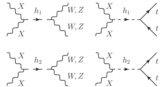
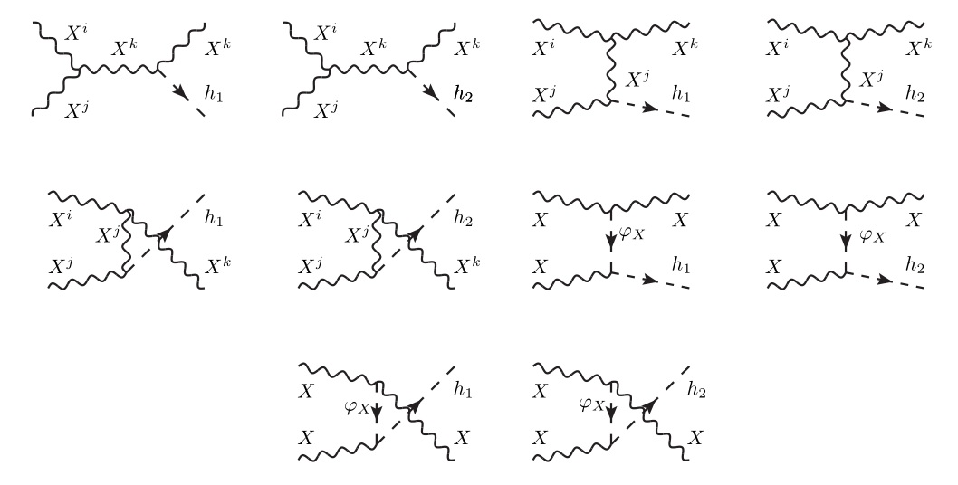
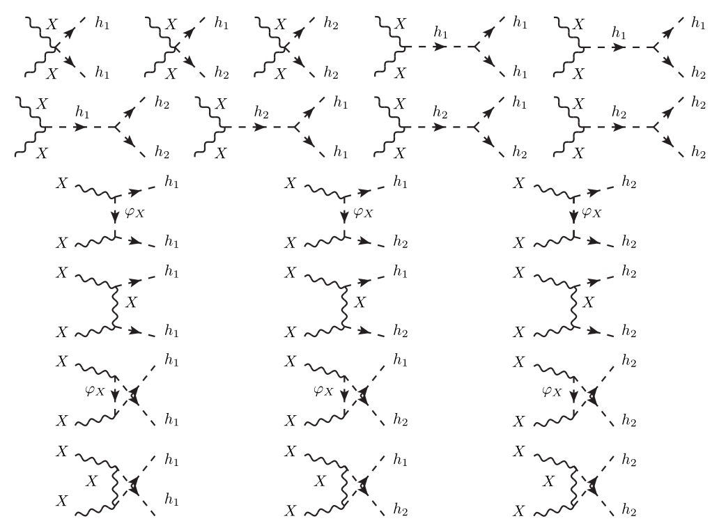
We assume that DM is a thermal relic, so we are going to describe which processes are important during DM freeze-out. We have to consider the annihilation processes, i.e. XXhihj𝑋𝑋subscript𝑖subscript𝑗XX\rightarrow h_{i}h_{j} (Figure 1), XXWW𝑋𝑋𝑊𝑊XX\rightarrow WW, XXZZ𝑋𝑋𝑍𝑍XX\rightarrow ZZ and XXtt¯𝑋𝑋𝑡¯𝑡XX\rightarrow t\bar{t} (Figure 2). Moreover, we have to take in account the semiannihilation processes XXXhi𝑋𝑋𝑋subscript𝑖XX\rightarrow Xh_{i} (Figure 3). Since DM is cold, we considered only the non-relativistic limit.
Refer to caption
Figure 1: Feynman diagrams for the annihilation process of the DM with scalars in the final state.
Refer to caption
Figure 2: Feynman diagrams for the annihilation process of the DM with W, Z or Top quark in the final state.
Refer to caption
Figure 3: Feynman diagrams for the semiannihilation process of the DM.

There are six contributions to the annihilation cross-section: the first one has two h1subscript1h_{1} particles in the final state, the third one has two h2subscript2h_{2} particles, while the second one has one of each scalar. The last three contributions are related respectively to the production of a couple of W, a couple of Z or a couple of Top quarks.

σvannh1,h1=gX2110592πMX3MX2Mh22×(16gX2cos4α(11Mh2428Mh22MX2+44MX4)(Mh222MX2)2+8gXMXcos2α(Mh2210MX2)𝒜1(4MX2Mh12)(Mh224MX2)(Mh222MX2)+3MX2𝒜12(Mh124MX2)2(Mh224MX2)2)𝜎superscriptsubscript𝑣annsubscript1subscript1superscriptsubscript𝑔𝑋2110592𝜋superscriptsubscript𝑀𝑋3superscriptsubscript𝑀𝑋2superscriptsubscript𝑀subscript2216superscriptsubscript𝑔𝑋2superscript4𝛼11superscriptsubscript𝑀subscript2428superscriptsubscript𝑀subscript22superscriptsubscript𝑀𝑋244superscriptsubscript𝑀𝑋4superscriptsuperscriptsubscript𝑀subscript222superscriptsubscript𝑀𝑋228subscript𝑔𝑋subscript𝑀𝑋superscript2𝛼superscriptsubscript𝑀subscript2210superscriptsubscript𝑀𝑋2subscript𝒜14superscriptsubscript𝑀𝑋2superscriptsubscript𝑀subscript12superscriptsubscript𝑀subscript224superscriptsubscript𝑀𝑋2superscriptsubscript𝑀subscript222superscriptsubscript𝑀𝑋23superscriptsubscript𝑀𝑋2superscriptsubscript𝒜12superscriptsuperscriptsubscript𝑀subscript124superscriptsubscript𝑀𝑋22superscriptsuperscriptsubscript𝑀subscript224superscriptsubscript𝑀𝑋22\displaystyle\begin{split}\sigma v_{\text{ann}}^{h_{1},h_{1}}&=\frac{g_{X}^{2}}{110592\pi M_{X}^{3}}\sqrt{M_{X}^{2}-M_{h_{2}}^{2}}\\ &\times\left(\frac{16g_{X}^{2}\cos^{4}\alpha\left(11M_{h_{2}}^{4}-28M_{h_{2}}^{2}M_{X}^{2}+44M_{X}^{4}\right)}{\left(M_{h_{2}}^{2}-2M_{X}^{2}\right)^{2}}\right.\\ &+\frac{8g_{X}M_{X}\cos^{2}\alpha\left(M_{h_{2}}^{2}-10M_{X}^{2}\right)\mathcal{A}_{1}}{\left(4M_{X}^{2}-M_{h_{1}}^{2}\right)\left(M_{h_{2}}^{2}-4M_{X}^{2}\right)\left(M_{h_{2}}^{2}-2M_{X}^{2}\right)}\\ &\left.+\frac{3M_{X}^{2}\mathcal{A}_{1}^{2}}{\left(M_{h_{1}}^{2}-4M_{X}^{2}\right)^{2}\left(M_{h_{2}}^{2}-4M_{X}^{2}\right)^{2}}\right)\end{split} (15)
𝒜1=w(λHS6λS)(3Mh12+Mh2216MX2)+2vsin(2α)(Mh12(6λH3λHS)Mh22(6λH+λHS)+16λHSMX2)4wcos(2α)(6λSMh12+λHSMh224MX2(λHS+6λS))3vsin(4α)(2λH+λHS)(Mh12Mh22)3wcos(4α)(λHS+2λS)(Mh12Mh22)subscript𝒜1𝑤subscript𝜆𝐻𝑆6subscript𝜆𝑆3superscriptsubscript𝑀subscript12superscriptsubscript𝑀subscript2216superscriptsubscript𝑀𝑋22𝑣2𝛼superscriptsubscript𝑀subscript126subscript𝜆𝐻3subscript𝜆𝐻𝑆superscriptsubscript𝑀subscript226subscript𝜆𝐻subscript𝜆𝐻𝑆16subscript𝜆𝐻𝑆superscriptsubscript𝑀𝑋24𝑤2𝛼6subscript𝜆𝑆superscriptsubscript𝑀subscript12subscript𝜆𝐻𝑆superscriptsubscript𝑀subscript224superscriptsubscript𝑀𝑋2subscript𝜆𝐻𝑆6subscript𝜆𝑆3𝑣4𝛼2subscript𝜆𝐻subscript𝜆𝐻𝑆superscriptsubscript𝑀subscript12superscriptsubscript𝑀subscript223𝑤4𝛼subscript𝜆𝐻𝑆2subscript𝜆𝑆superscriptsubscript𝑀subscript12superscriptsubscript𝑀subscript22\displaystyle\begin{split}\mathcal{A}_{1}&=w(\lambda_{HS}-6\lambda_{S})\left(3M_{h_{1}}^{2}+M_{h_{2}}^{2}-16M_{X}^{2}\right)\\ &+2v\sin(2\alpha)\left(M_{h_{1}}^{2}(6\lambda_{H}-3\lambda_{HS})-M_{h_{2}}^{2}(6\lambda_{H}+\lambda_{HS})+16\lambda_{HS}M_{X}^{2}\right)\\ &-4w\cos(2\alpha)\left(6\lambda_{S}M_{h_{1}}^{2}+\lambda_{HS}M_{h_{2}}^{2}-4M_{X}^{2}(\lambda_{HS}+6\lambda_{S})\right)\\ &-3v\sin(4\alpha)(2\lambda_{H}+\lambda_{HS})\left(M_{h_{1}}^{2}-M_{h_{2}}^{2}\right)\\ &-3w\cos(4\alpha)(\lambda_{HS}+2\lambda_{S})\left(M_{h_{1}}^{2}-M_{h_{2}}^{2}\right)\end{split} (16)
σvannh1,h2=gX2221184πMX8Mh142Mh12(Mh22+4MX2)+(Mh224MX2)2×(gX2sin2(2α)(Mh12+Mh224MX2)2(224MX6(Mh12+Mh22)12MX2(Mh12Mh22)2(Mh12+Mh22)+(Mh12Mh22)4+MX4(92Mh148Mh12Mh22+92Mh24)+704MX8)+2gXMX3sin(2α)(Mh14+Mh242Mh12(Mh22+MX2)2Mh22MX2+40MX4)𝒜2(Mh124MX2)(4MX2Mh22)(Mh12+Mh224MX2)+3MX6𝒜22(Mh124MX2)2(Mh224MX2)2)𝜎superscriptsubscript𝑣annsubscript1subscript2superscriptsubscript𝑔𝑋2221184𝜋superscriptsubscript𝑀𝑋8superscriptsubscript𝑀subscript142superscriptsubscript𝑀subscript12superscriptsubscript𝑀subscript224superscriptsubscript𝑀𝑋2superscriptsuperscriptsubscript𝑀subscript224superscriptsubscript𝑀𝑋22superscriptsubscript𝑔𝑋2superscript22𝛼superscriptsuperscriptsubscript𝑀subscript12superscriptsubscript𝑀subscript224superscriptsubscript𝑀𝑋22224superscriptsubscript𝑀𝑋6superscriptsubscript𝑀subscript12superscriptsubscript𝑀subscript2212superscriptsubscript𝑀𝑋2superscriptsuperscriptsubscript𝑀subscript12superscriptsubscript𝑀subscript222superscriptsubscript𝑀subscript12superscriptsubscript𝑀subscript22superscriptsuperscriptsubscript𝑀subscript12superscriptsubscript𝑀subscript224superscriptsubscript𝑀𝑋492superscriptsubscript𝑀subscript148superscriptsubscript𝑀subscript12superscriptsubscript𝑀subscript2292superscriptsubscript𝑀subscript24704superscriptsubscript𝑀𝑋82subscript𝑔𝑋superscriptsubscript𝑀𝑋32𝛼superscriptsubscript𝑀subscript14superscriptsubscript𝑀subscript242superscriptsubscript𝑀subscript12superscriptsubscript𝑀subscript22superscriptsubscript𝑀𝑋22superscriptsubscript𝑀subscript22superscriptsubscript𝑀𝑋240superscriptsubscript𝑀𝑋4subscript𝒜2superscriptsubscript𝑀subscript124superscriptsubscript𝑀𝑋24superscriptsubscript𝑀𝑋2superscriptsubscript𝑀subscript22superscriptsubscript𝑀subscript12superscriptsubscript𝑀subscript224superscriptsubscript𝑀𝑋23superscriptsubscript𝑀𝑋6superscriptsubscript𝒜22superscriptsuperscriptsubscript𝑀subscript124superscriptsubscript𝑀𝑋22superscriptsuperscriptsubscript𝑀subscript224superscriptsubscript𝑀𝑋22\displaystyle\begin{split}&\sigma v_{\text{ann}}^{h_{1},h_{2}}=\frac{g_{X}^{2}}{221184\pi M_{X}^{8}}\sqrt{M_{h_{1}}^{4}-2M_{h_{1}}^{2}\left(M_{h_{2}}^{2}+4M_{X}^{2}\right)+\left(M_{h_{2}}^{2}-4M_{X}^{2}\right)^{2}}\\ &\times\left(\frac{g_{X}^{2}\sin^{2}(2\alpha)}{\left(M_{h_{1}}^{2}+M_{h_{2}}^{2}-4M_{X}^{2}\right)^{2}}\right.\\ &\qquad\left(-224M_{X}^{6}\left(M_{h_{1}}^{2}+M_{h_{2}}^{2}\right)-12M_{X}^{2}\left(M_{h_{1}}^{2}-M_{h_{2}}^{2}\right)^{2}\left(M_{h_{1}}^{2}+M_{h_{2}}^{2}\right)\right.\\ &\left.\qquad+\left(M_{h_{1}}^{2}-M_{h_{2}}^{2}\right)^{4}+M_{X}^{4}\left(92M_{h_{1}}^{4}-8M_{h_{1}}^{2}M_{h_{2}}^{2}+92M_{h_{2}}^{4}\right)+704M_{X}^{8}\right)\\ &+\frac{2g_{X}M_{X}^{3}\sin(2\alpha)\left(M_{h_{1}}^{4}+M_{h_{2}}^{4}-2M_{h_{1}}^{2}\left(M_{h_{2}}^{2}+M_{X}^{2}\right)-2M_{h_{2}}^{2}M_{X}^{2}+40M_{X}^{4}\right)\mathcal{A}_{2}}{\left(M_{h_{1}}^{2}-4M_{X}^{2}\right)\left(4M_{X}^{2}-M_{h_{2}}^{2}\right)\left(M_{h_{1}}^{2}+M_{h_{2}}^{2}-4M_{X}^{2}\right)}\\ &+\left.\frac{3M_{X}^{6}\mathcal{A}_{2}^{2}}{\left(M_{h_{1}}^{2}-4M_{X}^{2}\right)^{2}\left(M_{h_{2}}^{2}-4M_{X}^{2}\right)^{2}}\right)\end{split} (17)
𝒜2=v(6λHλHS)(Mh12Mh22)4λHSvcos(2α)(Mh12+Mh228MX2)+2wsin(2α)(λHS+6λS)(Mh12+Mh228MX2)3vcos(4α)(2λH+λHS)(Mh12Mh22)+3wsin(4α)(λHS+2λS)(Mh12Mh22)subscript𝒜2𝑣6subscript𝜆𝐻subscript𝜆𝐻𝑆superscriptsubscript𝑀subscript12superscriptsubscript𝑀subscript224subscript𝜆𝐻𝑆𝑣2𝛼superscriptsubscript𝑀subscript12superscriptsubscript𝑀subscript228superscriptsubscript𝑀𝑋22𝑤2𝛼subscript𝜆𝐻𝑆6subscript𝜆𝑆superscriptsubscript𝑀subscript12superscriptsubscript𝑀subscript228superscriptsubscript𝑀𝑋23𝑣4𝛼2subscript𝜆𝐻subscript𝜆𝐻𝑆superscriptsubscript𝑀subscript12superscriptsubscript𝑀subscript223𝑤4𝛼subscript𝜆𝐻𝑆2subscript𝜆𝑆superscriptsubscript𝑀subscript12superscriptsubscript𝑀subscript22\displaystyle\begin{split}\mathcal{A}_{2}&=v(6\lambda_{H}-\lambda_{HS})\left(M_{h_{1}}^{2}-M_{h_{2}}^{2}\right)\\ &-4\lambda_{HS}v\cos(2\alpha)\left(M_{h_{1}}^{2}+M_{h_{2}}^{2}-8M_{X}^{2}\right)\\ &+2w\sin(2\alpha)(\lambda_{HS}+6\lambda_{S})\left(M_{h_{1}}^{2}+M_{h_{2}}^{2}-8M_{X}^{2}\right)\\ &-3v\cos(4\alpha)(2\lambda_{H}+\lambda_{HS})\left(M_{h_{1}}^{2}-M_{h_{2}}^{2}\right)\\ &+3w\sin(4\alpha)(\lambda_{HS}+2\lambda_{S})\left(M_{h_{1}}^{2}-M_{h_{2}}^{2}\right)\end{split} (18)
σvannh2,h2=gX2110592πMX3MX2Mh12×(16gX2sin4α(11Mh1428Mh12MX2+44MX4)(Mh122MX2)28gXMXsin2α(10MX2Mh12)𝒜3(Mh124MX2)(Mh122MX2)(4MX2Mh22)+3MX2𝒜32(Mh124MX2)2(Mh224MX2)2)𝜎superscriptsubscript𝑣annsubscript2subscript2superscriptsubscript𝑔𝑋2110592𝜋superscriptsubscript𝑀𝑋3superscriptsubscript𝑀𝑋2superscriptsubscript𝑀subscript1216superscriptsubscript𝑔𝑋2superscript4𝛼11superscriptsubscript𝑀subscript1428superscriptsubscript𝑀subscript12superscriptsubscript𝑀𝑋244superscriptsubscript𝑀𝑋4superscriptsuperscriptsubscript𝑀subscript122superscriptsubscript𝑀𝑋228subscript𝑔𝑋subscript𝑀𝑋superscript2𝛼10superscriptsubscript𝑀𝑋2superscriptsubscript𝑀subscript12subscript𝒜3superscriptsubscript𝑀subscript124superscriptsubscript𝑀𝑋2superscriptsubscript𝑀subscript122superscriptsubscript𝑀𝑋24superscriptsubscript𝑀𝑋2superscriptsubscript𝑀subscript223superscriptsubscript𝑀𝑋2superscriptsubscript𝒜32superscriptsuperscriptsubscript𝑀subscript124superscriptsubscript𝑀𝑋22superscriptsuperscriptsubscript𝑀subscript224superscriptsubscript𝑀𝑋22\displaystyle\begin{split}\sigma v_{\text{ann}}^{h_{2},h_{2}}&=\frac{g_{X}^{2}}{110592\pi M_{X}^{3}}\sqrt{M_{X}^{2}-M_{h_{1}}^{2}}\\ &\times\left(\frac{16g_{X}^{2}\sin^{4}\alpha\left(11M_{h_{1}}^{4}-28M_{h_{1}}^{2}M_{X}^{2}+44M_{X}^{4}\right)}{\left(M_{h_{1}}^{2}-2M_{X}^{2}\right)^{2}}\right.\\ &-\frac{8g_{X}M_{X}\sin^{2}\alpha\left(10M_{X}^{2}-M_{h_{1}}^{2}\right)\mathcal{A}_{3}}{\left(M_{h_{1}}^{2}-4M_{X}^{2}\right)\left(M_{h_{1}}^{2}-2M_{X}^{2}\right)\left(4M_{X}^{2}-M_{h_{2}}^{2}\right)}\\ &+\left.\frac{3M_{X}^{2}\mathcal{A}_{3}^{2}}{\left(M_{h_{1}}^{2}-4M_{X}^{2}\right)^{2}\left(M_{h_{2}}^{2}-4M_{X}^{2}\right)^{2}}\right)\end{split} (19)
𝒜3=w(λHS6λS)(Mh12+3Mh2216MX2)+2vsin(2α)(Mh12(6λH+λHS)+Mh22(3λHS6λH)16λHSMX2)+4wcos(2α)(λHSMh12+6λSMh224MX2(λHS+6λS))+3vsin(4α)(2λH+λHS)(Mh12Mh22)+3wcos(4α)(λHS+2λS)(Mh12Mh22)subscript𝒜3𝑤subscript𝜆𝐻𝑆6subscript𝜆𝑆superscriptsubscript𝑀subscript123superscriptsubscript𝑀subscript2216superscriptsubscript𝑀𝑋22𝑣2𝛼superscriptsubscript𝑀subscript126subscript𝜆𝐻subscript𝜆𝐻𝑆superscriptsubscript𝑀subscript223subscript𝜆𝐻𝑆6subscript𝜆𝐻16subscript𝜆𝐻𝑆superscriptsubscript𝑀𝑋24𝑤2𝛼subscript𝜆𝐻𝑆superscriptsubscript𝑀subscript126subscript𝜆𝑆superscriptsubscript𝑀subscript224superscriptsubscript𝑀𝑋2subscript𝜆𝐻𝑆6subscript𝜆𝑆3𝑣4𝛼2subscript𝜆𝐻subscript𝜆𝐻𝑆superscriptsubscript𝑀subscript12superscriptsubscript𝑀subscript223𝑤4𝛼subscript𝜆𝐻𝑆2subscript𝜆𝑆superscriptsubscript𝑀subscript12superscriptsubscript𝑀subscript22\displaystyle\begin{split}\mathcal{A}_{3}&=w(\lambda_{HS}-6\lambda_{S})\left(M_{h_{1}}^{2}+3M_{h_{2}}^{2}-16M_{X}^{2}\right)\\ &+2v\sin(2\alpha)\left(M_{h_{1}}^{2}(6\lambda_{H}+\lambda_{HS})+M_{h_{2}}^{2}(3\lambda_{HS}-6\lambda_{H})-16\lambda_{HS}M_{X}^{2}\right)\\ &+4w\cos(2\alpha)\left(\lambda_{HS}M_{h_{1}}^{2}+6\lambda_{S}M_{h_{2}}^{2}-4M_{X}^{2}(\lambda_{HS}+6\lambda_{S})\right)\\ &+3v\sin(4\alpha)(2\lambda_{H}+\lambda_{HS})\left(M_{h_{1}}^{2}-M_{h_{2}}^{2}\right)\\ &+3w\cos(4\alpha)(\lambda_{HS}+2\lambda_{S})\left(M_{h_{1}}^{2}-M_{h_{2}}^{2}\right)\end{split} (20)
σvannWW=gX2sin2(2α)(Mh12Mh22)2(3MW44MW2MX2+4MX4)MX2MW2288πMXv2(Mh124MX2)2(Mh224MX2)2𝜎superscriptsubscript𝑣ann𝑊𝑊superscriptsubscript𝑔𝑋2superscript22𝛼superscriptsuperscriptsubscript𝑀subscript12superscriptsubscript𝑀subscript2223superscriptsubscript𝑀𝑊44superscriptsubscript𝑀𝑊2superscriptsubscript𝑀𝑋24superscriptsubscript𝑀𝑋4superscriptsubscript𝑀𝑋2superscriptsubscript𝑀𝑊2288𝜋subscript𝑀𝑋superscript𝑣2superscriptsuperscriptsubscript𝑀subscript124superscriptsubscript𝑀𝑋22superscriptsuperscriptsubscript𝑀subscript224superscriptsubscript𝑀𝑋22\sigma v_{\text{ann}}^{WW}=\frac{g_{X}^{2}\sin^{2}(2\alpha)\left(M_{h_{1}}^{2}-M_{h_{2}}^{2}\right)^{2}\left(3M_{W}^{4}-4M_{W}^{2}M_{X}^{2}+4M_{X}^{4}\right)\sqrt{M_{X}^{2}-M_{W}^{2}}}{288\pi M_{X}v^{2}\left(M_{h_{1}}^{2}-4M_{X}^{2}\right)^{2}\left(M_{h_{2}}^{2}-4M_{X}^{2}\right)^{2}} (21)
σvannZZ=gX2sin2(2α)(Mh12Mh22)2(3MZ44MX2MZ2+4MX4)MX2MZ2576πMXv2(Mh124MX2)2(Mh224MX2)2𝜎superscriptsubscript𝑣ann𝑍𝑍superscriptsubscript𝑔𝑋2superscript22𝛼superscriptsuperscriptsubscript𝑀subscript12superscriptsubscript𝑀subscript2223superscriptsubscript𝑀𝑍44superscriptsubscript𝑀𝑋2superscriptsubscript𝑀𝑍24superscriptsubscript𝑀𝑋4superscriptsubscript𝑀𝑋2superscriptsubscript𝑀𝑍2576𝜋subscript𝑀𝑋superscript𝑣2superscriptsuperscriptsubscript𝑀subscript124superscriptsubscript𝑀𝑋22superscriptsuperscriptsubscript𝑀subscript224superscriptsubscript𝑀𝑋22\sigma v_{\text{ann}}^{ZZ}=\frac{g_{X}^{2}\sin^{2}(2\alpha)\left(M_{h_{1}}^{2}-M_{h_{2}}^{2}\right)^{2}\left(3M_{Z}^{4}-4M_{X}^{2}M_{Z}^{2}+4M_{X}^{4}\right)\sqrt{M_{X}^{2}-M_{Z}^{2}}}{576\pi M_{X}v^{2}\left(M_{h_{1}}^{2}-4M_{X}^{2}\right)^{2}\left(M_{h_{2}}^{2}-4M_{X}^{2}\right)^{2}} (22)
σvannTT=gX2sin2(2α)MT2(Mh12Mh22)2(MT2MX2)MX2MT2288πMXv2(Mh124MX2)2(Mh224MX2)2𝜎superscriptsubscript𝑣ann𝑇𝑇superscriptsubscript𝑔𝑋2superscript22𝛼superscriptsubscript𝑀𝑇2superscriptsuperscriptsubscript𝑀subscript12superscriptsubscript𝑀subscript222superscriptsubscript𝑀𝑇2superscriptsubscript𝑀𝑋2superscriptsubscript𝑀𝑋2superscriptsubscript𝑀𝑇2288𝜋subscript𝑀𝑋superscript𝑣2superscriptsuperscriptsubscript𝑀subscript124superscriptsubscript𝑀𝑋22superscriptsuperscriptsubscript𝑀subscript224superscriptsubscript𝑀𝑋22\sigma v_{\text{ann}}^{TT}=\frac{g_{X}^{2}\sin^{2}(2\alpha)M_{T}^{2}\left(M_{h_{1}}^{2}-M_{h_{2}}^{2}\right)^{2}\left(M_{T}^{2}-M_{X}^{2}\right)\sqrt{M_{X}^{2}-M_{T}^{2}}}{288\pi M_{X}v^{2}\left(M_{h_{1}}^{2}-4M_{X}^{2}\right)^{2}\left(M_{h_{2}}^{2}-4M_{X}^{2}\right)^{2}} (23)

The semiannihilation cross section is

σsemiannv=gX4(Mh1410Mh12MX2+9MX4)3/2sin2(α)128πMX4(Mh123MX2)2+gX4(Mh2410Mh22MX2+9MX4)3/2cos2(α)128πMX4(Mh223MX2)2.subscript𝜎semiann𝑣superscriptsubscript𝑔𝑋4superscriptsuperscriptsubscript𝑀subscript1410superscriptsubscript𝑀subscript12superscriptsubscript𝑀𝑋29superscriptsubscript𝑀𝑋432superscript2𝛼128𝜋superscriptsubscript𝑀𝑋4superscriptsuperscriptsubscript𝑀subscript123superscriptsubscript𝑀𝑋22superscriptsubscript𝑔𝑋4superscriptsuperscriptsubscript𝑀subscript2410superscriptsubscript𝑀subscript22superscriptsubscript𝑀𝑋29superscriptsubscript𝑀𝑋432superscript2𝛼128𝜋superscriptsubscript𝑀𝑋4superscriptsuperscriptsubscript𝑀subscript223superscriptsubscript𝑀𝑋22\displaystyle\begin{split}\sigma_{\text{semiann}}v&=\frac{g_{X}^{4}\left(M_{h_{1}}^{4}-10M_{h_{1}}^{2}M_{X}^{2}+9M_{X}^{4}\right)^{3/2}\sin^{2}(\alpha)}{128\pi M_{X}^{4}\left(M_{h_{1}}^{2}-3M_{X}^{2}\right)^{2}}\\ &+\frac{g_{X}^{4}\left(M_{h_{2}}^{4}-10M_{h_{2}}^{2}M_{X}^{2}+9M_{X}^{4}\right)^{3/2}\cos^{2}(\alpha)}{128\pi M_{X}^{4}\left(M_{h_{2}}^{2}-3M_{X}^{2}\right)^{2}}.\end{split} (24)

We observe that in the limit of small λHSsubscript𝜆𝐻𝑆\lambda_{HS}, we get the same result of the approximated computation of [22].

Calling σannsubscript𝜎ann\sigma_{\text{ann}} and σsemiannsubscript𝜎semiann\sigma_{\text{semiann}} the non-relativistic cross sections of these processes, we can say the experimental Dark Matter abundance is reproduced if [22, 23]

σannv+12σsemiannv=2.2×1026cm3/s=1.83×109GeV2,subscript𝜎ann𝑣12subscript𝜎semiann𝑣2.2superscript1026superscriptcm3s1.83superscript109superscriptGeV2\sigma_{\text{ann}}v+\frac{1}{2}\sigma_{\text{semiann}}v=2.2\times 10^{-26}\text{cm}^{3}/\text{s}=1.83\times 10^{-9}\text{GeV}^{-2}, (25)

where v𝑣v is the relative velocity between the initial particles. We added a factor 1/2121/2 for the semi-annihilations because the number of DM particles drops only by one unit, so their contribution to the total annihilation of the DM is just one half of the contribution of the annihilations. We averaged these cross sections over the polarizations of the vectors and over their SU(2)XX{}_{\text{X}} indices.

3.5 Corrections to the VEV of the Higgs

The VEV of the Higgs is fixed by the amplitude of the muon decay process. The relation between the Higgs VEV and the Fermi constant GFsubscript𝐺𝐹G_{F} is

GF2=12v2(1+Δr),subscript𝐺𝐹212superscript𝑣21Δ𝑟\frac{G_{F}}{\sqrt{2}}=\frac{1}{2v^{2}}(1+\Delta r), (26)

where ΔrΔ𝑟\Delta r encloses all the contributions given by the corrections to the W boson propagator. In tree-level approximation we have Δr=0Δ𝑟0\Delta r=0. The experimental value of the Fermi constant is 1.16637×10⁵GeV21.16637superscript105superscriptGeV21.16637\times 10^{-5}\text{GeV}^{-2}, so, considering only tree-level diagrams we obtain v246.22 GeVsimilar-to-or-equals𝑣246.22 GeVv\simeq 246.22\text{ GeV} from the previous relation.

We include one-loop corrections: ΔrΔ𝑟\Delta r is given by

Δr(1loop)=ΔrSM(MhMh1)cos2α+ΔrSM(MhMh2)sin2α.Δsuperscript𝑟(1loop)Δsuperscript𝑟SMsubscript𝑀subscript𝑀subscript1superscript2𝛼Δsuperscript𝑟SMsubscript𝑀subscript𝑀subscript2superscript2𝛼\Delta r^{\text{(1loop)}}=\Delta r^{\text{SM}}(M_{h}\rightarrow M_{h_{1}})\cos^{2}\alpha+\Delta r^{\text{SM}}(M_{h}\rightarrow M_{h_{2}})\sin^{2}\alpha. (27)

where ΔrSMΔsuperscript𝑟SM\Delta r^{\text{SM}} is the known SM result [24] in the Landau gauge ξW=ξZ=ξX=0subscript𝜉𝑊subscript𝜉𝑍subscript𝜉𝑋0\xi_{W}=\xi_{Z}=\xi_{X}=0.

4 Results

Now we have to write a system of equations, imposing that our observables agree with the experimental data. We introduced six parameters in this model, but the presently available observables that we computed give us only five conditions, so we choose gXsubscript𝑔𝑋g_{X} as the only free parameter. We find the values of λHsubscript𝜆𝐻\lambda_{H}, λHSsubscript𝜆𝐻𝑆\lambda_{HS}, μ2superscriptsuperscript𝜇2{\mu^{\ast}}^{2}, v𝑣v and w𝑤w:

{V1looph=0V1loops=0Mh2=mh2+ΔΠ(p2)=(125.6GeV)21v22(1+Δr(1loop))=GF=1.16637×10⁵GeV2σannv+12σsemiannv=2.2×1026cm3/s=1.83×109GeV2casessuperscript𝑉1loop0otherwisesuperscript𝑉1loop𝑠0otherwisesuperscriptsubscript𝑀2superscriptsubscript𝑚2ΔΠsuperscript𝑝2superscript125.6GeV2otherwise1superscript𝑣221Δsuperscript𝑟(1loop)subscript𝐺𝐹1.16637superscript105superscriptGeV2otherwisesubscript𝜎ann𝑣12subscript𝜎semiann𝑣2.2superscript1026superscriptcm3s1.83superscript109superscriptGeV2otherwise\begin{cases}\frac{\partial V^{\text{1loop}}}{\partial h}=0\\ \frac{\partial V^{\text{1loop}}}{\partial s}=0\\ M_{h}^{2}=m_{h}^{2}+\Delta\Pi(p^{2})=(125.6\text{GeV})^{2}\\ \frac{1}{v^{2}\sqrt{2}}(1+\Delta r^{\text{(1loop)}})=G_{F}=1.16637\times 10^{-5}\text{GeV}^{-2}\\ \sigma_{\text{ann}}v+\frac{1}{2}\sigma_{\text{semiann}}v=2.2\times 10^{-26}\text{cm}^{3}/\text{s}=1.83\times 10^{-9}\text{GeV}^{-2}\end{cases} (28)

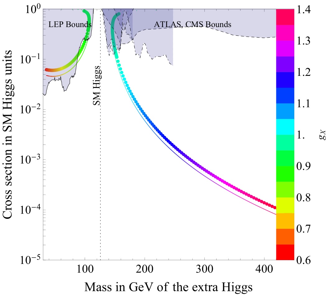
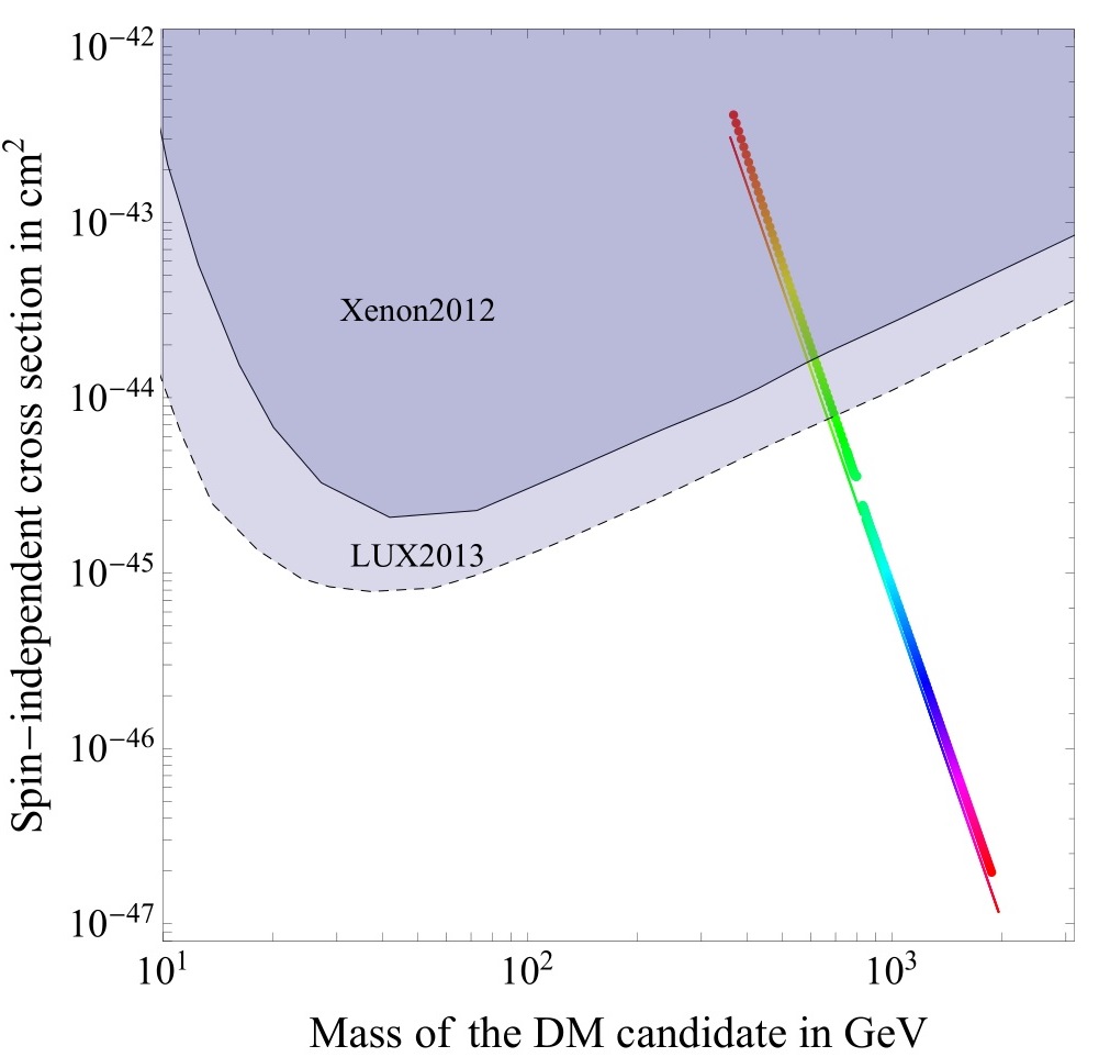
This system has to be solved in two cases, because we don’t know which of the eigenvalues of the one-loop mass matrix corresponds to the Higgs. Then, we have to compute the solution for every value of gXsubscript𝑔𝑋g_{X}. We have a set of solutions showing us the values of the parameters of the model as function of gXsubscript𝑔𝑋g_{X}. With these data we plot the predicted cross section for the production of the new scalar as a function of the mass of the scalar itself, and a diagram of the spin-independent cross section for direct detection of the Dark Matter as a function of the mass of the DM particle and of the free parameter.

In the limit where we are taking in account only gauge interactions, our results reproduce those of [22].

The plots report the bounds given by LEP experiments for energies lower than the Higgs mass and by ATLAS and CMS experiments for greater energies. The bounds of the LEP experiments are the 95% confidence level of the ratio σ/σSM𝜎superscript𝜎SM\sigma/\sigma^{\text{SM}}, where σ𝜎\sigma is the measured production cross section of the Higgs, while σSMsuperscript𝜎SM\sigma^{\text{SM}} is its theoretical value for the SM [25]. The bounds given by ATLAS and CMS at large mass are the 95% CL upper limits on the production cross section of a Higgs boson: hWW𝑊𝑊h\rightarrow WW searches are plotted as dashed curves and hWW𝑊𝑊h\rightarrow WW searches as dot-dashed curves [1, 26, 27]. Below, in Figure 4, we present the spin independent cross section for direct detection in the complete case. The bounds are the 90% confidence level of spin-independent DM-nucleon scattering cross section. The model is not excluded by XENON2012 and LUX2013 data for gX0.8greater-than-or-equivalent-tosubscript𝑔𝑋0.8g_{X}\gtrsim 0.8 [28, 29].

Refer to caption
Refer to caption
Figure 4: Our final result: above, the prediction of the complete model for the production cross section of the new scalar. Below we report the prediction for the cross section for DM direct detection. These quantities are plotted as a function of the parameter gXsubscript𝑔𝑋g_{X}, that varies accordingly to the colors on the legend. For a comparison, in these diagrams we leave the data of the approximated case as smaller points. The grey areas are excluded by LEP or CMS and ATLAS experiments for the diagram above, while the bounds comes from XENON2012 and from LUX2013 experiments for the diagram below (see Section 4 for more detail on the bounds).

5 RGE analysis

After finding the values of the parameters of the model around the weak scale, now we have to explore the behaviour of these parameters at high energy. To do this, first we must find the renormalization group equations (RGEs) for the theory. We can get these equation starting from those of the Standard Model. In particular, the scalar quartic coupling has an extra term due to the interaction between the Higgs boson and the new scalar boson:

(4π)2dλHdlnμ=(12gt295g129g22)λH6gt4+27200g14+920g22g12+98g24+24λH2+2λHS2superscript4𝜋2𝑑subscript𝜆𝐻𝑑𝜇12superscriptsubscript𝑔𝑡295superscriptsubscript𝑔129superscriptsubscript𝑔22subscript𝜆𝐻6superscriptsubscript𝑔𝑡427200superscriptsubscript𝑔14920superscriptsubscript𝑔22superscriptsubscript𝑔1298superscriptsubscript𝑔2424superscriptsubscript𝜆𝐻22superscriptsubscript𝜆𝐻𝑆2(4\pi)^{2}\frac{d\lambda_{H}}{d\ln\mu}=(12g_{t}^{2}-\frac{9}{5}g_{1}^{2}-9g_{2}^{2})\lambda_{H}-6g_{t}^{4}+\frac{27}{200}g_{1}^{4}+\frac{9}{20}g_{2}^{2}g_{1}^{2}+\frac{9}{8}g_{2}^{4}+24\lambda_{H}^{2}+2\lambda_{HS}^{2} (29)

The new coupling constants RGEs are

(4π)2dgXdlnμ=436gX31(4π)22596gX5superscript4𝜋2𝑑subscript𝑔𝑋𝑑𝜇436superscriptsubscript𝑔𝑋31superscript4𝜋22596superscriptsubscript𝑔𝑋5(4\pi)^{2}\frac{dg_{X}}{d\ln\mu}=-\frac{43}{6}g_{X}^{3}-\frac{1}{(4\pi)^{2}}\frac{259}{6}g_{X}^{5} (30)
(4π)2dλHSdlnμ=λHS(6gt292gX2910g1292g22+12λH+12λS)4λHS2superscript4𝜋2𝑑subscript𝜆𝐻𝑆𝑑𝜇subscript𝜆𝐻𝑆6superscriptsubscript𝑔𝑡292superscriptsubscript𝑔𝑋2910superscriptsubscript𝑔1292superscriptsubscript𝑔2212subscript𝜆𝐻12subscript𝜆𝑆4superscriptsubscript𝜆𝐻𝑆2(4\pi)^{2}\frac{d\lambda_{HS}}{d\ln\mu}=\lambda_{HS}(6g_{t}^{2}-\frac{9}{2}g_{X}^{2}-\frac{9}{10}g_{1}^{2}-\frac{9}{2}g_{2}^{2}+12\lambda_{H}+12\lambda_{S})-4\lambda_{HS}^{2} (31)
(4π)2dλSdlnμ=9gX2λS+98gX4+2λHS2+24λS2superscript4𝜋2𝑑subscript𝜆𝑆𝑑𝜇9superscriptsubscript𝑔𝑋2subscript𝜆𝑆98superscriptsubscript𝑔𝑋42superscriptsubscript𝜆𝐻𝑆224superscriptsubscript𝜆𝑆2(4\pi)^{2}\frac{d\lambda_{S}}{d\ln\mu}=-9g_{X}^{2}\lambda_{S}+\frac{9}{8}g_{X}^{4}+2\lambda_{HS}^{2}+24\lambda_{S}^{2} (32)

The other RGEs of the SM are not affected by the new sector of this model, so they remain exactly the same. In our computation we set the mass the Higgs boson equal to 125.9 GeV and the Top quark mass equal to 173 GeV.

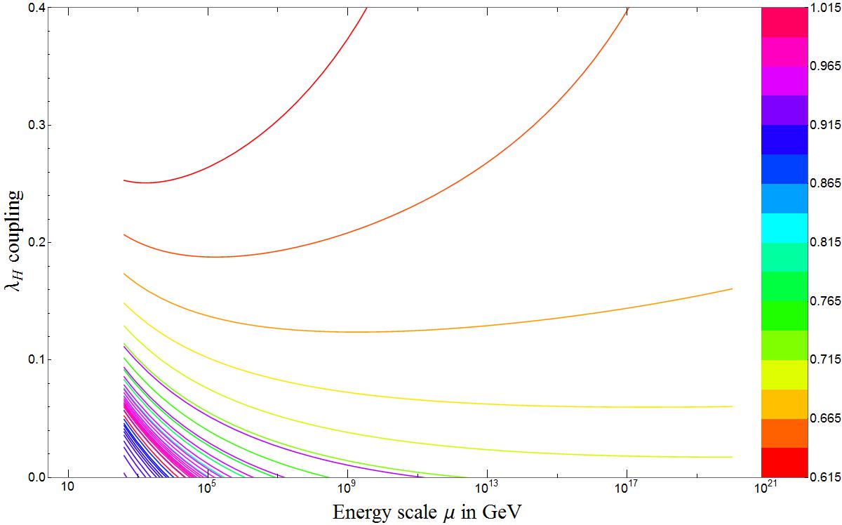
The results of are represented in Figure 5. First, we considered the case in which gX=1subscript𝑔𝑋1g_{X}=1 at the weak scale. We observe that for this value the problem of the vacuum instability of the SM is not solved yet. Since in this article we considered gXsubscript𝑔𝑋g_{X} as a free parameter of the theory, we studied if there is an interval for which the quartic coupling of the Higgs boson never becomes negative, for every energy scale. In the second diagram we see the running of the quartic scalar coupling from the weak scale to the Planck scale for a restricted range of values for the parameter gXsubscript𝑔𝑋g_{X}. We can say that the minimum is stable for gX0.695less-than-or-similar-tosubscript𝑔𝑋0.695g_{X}\lesssim 0.695 that corresponds to a mass of the new scalar lower than 53 GeV.
Refer to caption
Figure 5: Result of the RGE analysis for different values of the free parameter gXsubscript𝑔𝑋g_{X}: the running quartic coupling of this model remains positive at all the energy scales when gX0.695less-than-or-similar-tosubscript𝑔𝑋0.695g_{X}\lesssim 0.695. For bigger values of this parameter, that correspond to a heavier new scalar boson, there is an energy scale for which the quartic coupling λHsubscript𝜆𝐻\lambda_{H} becomes negative, causing the instability of the vacuum.

6 Conclusions

We considered an extension of the SM that describes the Dark Matter and proposes a reinterpretation to the hierarchy problem.

In the context of “finite naturalness”, we introduced a model without a mass term for the Higgs. The masses of the particles arise from a Coleman-Weinberg mechanism, so spontaneous symmetry breaking does not occur at tree-level, but is generated by the radiative corrections to the theory. We supposed that there is a new particle S𝑆S, scalar doublet under an extra group SU(2)X, and new vector bosons X𝑋X of the same gauge group. The only communication between this new sector and the SM is through the so-called “Higgs portal”, that is the quartic vertex between two Higgs fields and two S𝑆S fields. The VEVs of the two scalars are fixed by the one-loop potential; the interactions with the scalars give mass to all the particles of the model.

We introduced the vector boson X𝑋X of SU(2)X, that is a good candidate to represent the Dark Matter. It has a mass of about 1 TeV, and if we make a rough estimate, this is the order of magnitude of the scale where the mass of the DM particle is expected, assuming it is a thermal relict. Furthermore, this particle has to be stable. Some theories have to introduce special symmetries with the specific purpose of keeping the DM particle stable. In our model, X𝑋X vectors are automatically stable, because of the gauge symmetry and because of the particle content of the theory.

Another peculiarity of this simple model is the presence of only one free parameter. The other parameters introduced in the model are fixed by the experimental values of the DM cosmological abundance, of the Fermi constant and of the Higgs mass.

The original work presented in this article consisted in performing for the first time a precise computation of the predictions of the model for the LHC and for direct detection experiments. The new computation includes for the first time a full one-loop computation of the scalar masses and of the effective potential, and a full tree-level computation of the DM annihilations and semi-annihilations relevant for the thermal DM abundance.

In our computation the numerical solving algorithm of the system converges to an acceptable solution for a bigger number of values of the free parameter than the previous works on this model. For example, in the diagram of the direct dectection cross section of the DM of [22], there were no points for the values gX0.9subscript𝑔𝑋0.9g_{X}\approx 0.9, that corresponds to a mass of the new scalar almost equal to the Higgs mass.

Given the mass Mssubscript𝑀𝑠M_{s} of the extra scalar, the cross section for its production for LHC increases by a factor \approx1.3 with respect to the approximated computation. This cross section is compatible with the experiments in a small range around gX0.9subscript𝑔𝑋0.9g_{X}\approx 0.9 when the new scalar is lighter than Higgs, and for gX1.0greater-than-or-equivalent-tosubscript𝑔𝑋1.0g_{X}\gtrsim 1.0 when it is heavier.

From the LUX2013 and XENON2012 we get a constrain on the free parameter: the prediction for the DM direct detection is compatible with the bounds for gX0.8greater-than-or-equivalent-tosubscript𝑔𝑋0.8g_{X}\gtrsim 0.8, that corresponds to a mass of the DM particle 700greater-than-or-equivalent-toabsent700\gtrsim 700 GeV.

We considered also the behaviour of the coupling constant at high energy, studying their running through the RGEs. We can see that there are some values of the free parameter, that is the gauge coupling gXsubscript𝑔𝑋g_{X}, the Higgs quartic coupling stays automatically positive at all the energy scales: this case occurs for gX0.695less-than-or-similar-tosubscript𝑔𝑋0.695g_{X}\lesssim 0.695, that is for a new scalar lighter than 53 GeV. Obviously this case has already been disfavoured by the other analysis done in this article, so the question about the instability of the vacuum remains open, and more new physics is needed to solve this problem.

The collaborations of the new experiments LZ and XENON1T claim that their detectors will probe spin indipendent cross sections of the DM direct detection almost 2 or 3 orders of magnitude lower than the actual values reached by LUX and XENON100. This sensitivity will surely be enough to directly detect the new DM particle of this model in a mass range around 1 TeV. Considering the substantial increase in luminosity of LHC and simulations made by ATLAS and CMS (for example see [30]), we expect that the new run of the LHC will see the new scalar boson if it has a mass 200less-than-or-similar-toabsent200\lesssim 200 GeV.

Acknowledgments

We thank A. Strumia for the collaboration and for the useful discussions.

References

  • [1] ATLAS Collaboration, Observation of a new particle in the search for the Standard Model Higgs boson with the ATLAS detector at the LHC, Phys. Lett. B 716 (2012) 1 [arXiv:1207.7214].
  • [2] CMS Collaboration, Observation of a new boson at a mass of 125 GeV with the CMS experiment at the LHC, Phys. Lett. B 716 (2012) 30 [arXiv:1207.7235].
  • [3] G. ’t Hooft, Naturalness, Chiral Symmetry and Spontaneous Chiral Symmetry Breaking in Recent Developments in Gauge Theories, ISBN 978-0-306-40479-5.
  • [4] M. Farina, D. Pappadopulo and A. Strumia, A modified naturalness principle and its experimental tests, [arXiv:1303.7244]
  • [5] S.R. Coleman and E.J. Weinberg, Phys. Rev. D 7 (1973) 1888. E. Gildener and S. Weinberg, Phys.Rev.D 13 (1976) 3333.
  • [6] R. Hempfling, The Next-to-Minimal Coleman-Weinberg Model, Phys. Lett. B 379 (1996) 153 [hep-ph/9604278].
  • [7] J. P. Fatelo, J. M. Gerard, T. Hambye and J. Weyers, Symmetry Breaking Induced by Top Quark Loops Phys. Rev. Lett. 74 (1995) 492.
  • [8] T. Hambye, Phys. Lett. B 371 (1996) 87, Symmetry breaking induced by top quark loops from a model without scalar mass, [hep-ph/9510266].
  • [9] W. F. Chang, J. N. Ng and J. M. S. Wu, Phys. Rev. D 75 (2007) 115016, Shadow Higgs from a scale-invariant hidden U(1)s model [hep-ph/0701254].
  • [10] R. Foot, A. Kobakhidze and R. R. Volkas, Phys. Lett. B 655 (2007) 156 [arXiv:0704.1165].
  • [11] R. Foot, A. Kobakhidze, K. L. McDonald, R. R. Volkas, Electroweak Higgs as a pseudo-Goldstone boson of broken scale invariance, Phys. Rev. D 77 (2008) 035006 [arXiv:0709.2750].
  • [12] S. Iso, N. Okada, Y. Orikasa, The minimal B-L model naturally realized at TeV scale, Phys. Rev. D 80 (2009) 115007 [arXiv:0909.0128].
  • [13] S. Iso and Y. Orikasa, TeV Scale B-L model with a flat Higgs potential at the Planck scale – in view of the hierarchy problem PTEP 2013 (2013) 023B08 [arXiv:1210.2848].
  • [14] C. Englert, J. Jaeckel, V. V. Khoze and M. Spannowsky, Emergence of the Electroweak Scale through the Higgs Portal, [arXiv:1301.4224].
  • [15] E. J. Chun, S. Jung, and H. M. Lee, Radiative generation of the Higgs potential, Phys. Lett. B 725 (2013) 158 [arXiv:1304.5815].
  • [16] M. Cirelli, N. Fornengo and A. Strumia, Minimal Dark Matter, Nucl. Phys. B 753 (2006) 178 [hep-ph/0512090].
  • [17] M. Heikinheimo, A. Racioppi, M. Raidal, C. Spethmann and K. Tuominen, Physical Naturalness and Dynamical Breaking of Classical Scale Invariance, [arXiv:1304.7006].
  • [18] M. Heikinheimo, A. Racioppi, M. Raidal, C. Spethmann and K. Tuominen, Dark Supersymmetry, [arXiv:1305.4182.]
  • [19] E. Gabrielli, M. Heikinheimo, K. Kannike, A. Racioppi, M. Raidal, and C. Spethmann, Towards Completing the Standard Model: Vacuum Stability, EWSB and Dark Matter, [arXiv:1309.6632]
  • [20] T. Hambye, Hidden vector Dark Matter, [arXiv:0811.0172].
  • [21] C. D. Carone and R. Ramos, Classical scale-invariance, the electroweak scale and vector dark matter, Phys. Rev. D 88, n. 5, 055020 (2013) [arXiv:1307.8428].
  • [22] T. Hambye and A. Strumia, Dynamical generation of the weak and Dark Matter scale, [arXiv:1306.2329].
  • [23] Planck collaboration, Planck 2013 results. XVI. Cosmological parameters. [arXiv:1303.5076].
  • [24] A. Sirlin, R. Zucchini, Dependence of the Higgs coupling h¯MS¯subscript¯¯MS\bar{h}_{\overline{\text{MS}}} on mHsubscript𝑚𝐻m_{H} and the possible onset of new physics, Nuclear Physics B 266, 389
  • [25] ALEPH, DELPHI, L3 and OPAL Collaborations, The LEP Working Group for Higgs Boson Searches, Search for the Standard Model Higgs Boson at LEP, Physics Letters B 565 (2003), 61 [arXiv:hep-ex/0306033]
  • [26] CMS Collaboration, Observation of a new boson with mass near 125 GeV in pp collisions at sqrt(s) = 7 and 8 TeV, JHEP 06 (2013) 081, [arXiv:1303.4571].
  • [27] M. Flechl, on behalf of the ATLAS, CMS collaborations, BSM Higgs results from ATLAS and CMS, [arXiv:1307.4589]
  • [28] XENON100 Collaboration, Dark Matter Results from 225 Live Days of XENON100 Data, Phys. Rev. Lett. 109, 181301 (2012), [arXiv:1207.5988]
  • [29] LUX Collaboration, First results from the LUX dark matter experiment at the Stanford Underground Research Facility, Phys. Rev. Lett. 112, 091303 (2014) [arXiv:1310.8214]
  • [30] ATLAS Collaboration, Beyond-the-Standard-Model Higgs boson searches at a High-Luminosity LHC with ATLAS, ATLAS-PHYS-PUB-2013-016