Violation of Bell’s Inequalities with Classical Shimony-Wolf States: Theory and Experiment
Abstract
For many decades the word “entanglement” has been firmly attached to the world of quantum mechanics, as is the phrase “Bell violation”. Here we introduce Shimony-Wolf fields, entirely classical non-deterministic states, as a basis for entanglement and Bell analyses. Such fields are well known in coherence optics and are open to test. We present experimental results showing that Shimony-Wolf states exhibit strong classical Bell violation, in effect opening a way of examining a new sector of the boundary between quantum and classical physics.
pacs:
03.65.Ud, 42.79.Hp, 42.25.JaThe difference between classical and quantum phenomena is sometimes difficult to pin down because distinctions can be prescribed in a number of inequivalent ways. This is a reason for the notorious obscurity of the quantum-classical border. State superposition is an essential quantum attribute, but it is not exclusive to quantum physics since all linear wave phenomena share it. Entanglement is often regarded as the quintessentially non-classical aspect of the physical world, and a quantum-classical distinction is provided by Bell-violation experiments. Here we report a theoretical analysis and a related experiment regarding the quantum-classical border as probed by Bell tests with classical waves. We employ what we suggest can be named Shimony-Wolf fields or states for this purpose.
First we note that observations, demonstrations and even applications of non-quantum wave entanglement exist. They exploit non-separable correlations among two or more degrees of freedom (DOF) of optical wave fields. In the past few years such applications have achieved notable successes including the resolution of a long-standing open issue concerning Mueller matrices Simon-etal , unification of competing interpretations of degree of polarization Qian-EberlyOL , and application of the Bell measure as a new index of coherence in optics Kagalwala-etal . These developments followed even earlier explorations of non-separable DOF correlation, both theoretical and experimental, in optical wave fields Spreeuw ; Ghose-Samal01 ; Lee-ThomasPRL ; Borges-etal ; Goldin-etal .
Next we call attention to Shimony’s reviews Shimony of the
consequences of Bell’s inequalities. He identifies three facts of quantum
Nature that must be recognized by any system produced for testing. In
his words, these are:
(I) In any state of a physical system there are some
eventualities which have indefinite truth values.
(II) If an
operation is performed which forces an eventuality with indefinite
truth value to achieve definiteness […] the outcome is a matter of
chance.
(III) There are ‘entangled systems’ (in Schrödinger’s
phrase) which have the property that they constitute a composite
system in a pure state, while neither of them separately is in a pure
state. (Here by eventualities Shimony means measurement outcomes.)
As it happens, within the well-known classical theory of optical coherence (see Wolf Wolf59 ) there are statistical states that satisfy all three criteria. One quickly sees that the usual expression for the classical electric field vector of a transverse wave,
| (1) |
is an entangled combination of the DOF for polarization and transverse amplitude, and because the amplitudes are understood as stochastic variables, the field takes a definite value only when it is observed. Beyond its probabilistic indeterminacy, the in (1) shares other quantum attributes – it has the form of a quantum state and can be called a pure state in the same sense. It is really a bi-vector, linear in two vector spaces at once, lab space for and , and continuous function space for and . We will call it a Shimony-Wolf field or state.
By using Shimony-Wolf states we are departing from the recently observed applications of non-separable but also non-stochastic DOF correlations and make a test of their stochastic extensions and limitations. The boundary zone between classical and quantum physics is opened for examination in a new way. We can address questions such as: which features considered to be intrinsic to quantum theory can be fully replicated in a classical context? and what is the role of Bell inequalities for Shimony-Wolf states?
A prompt response to such questions could be to say that existing observations of Bell Inequality violations Freedman-Clauser ; Aspect-etal ; Ou-Mandel ; Shih-Alley ; Rowe-etal argue that classical systems are unable to provide the strong correlations predicted by quantum theory and attained when tested. The reply is that all such tests were made by particle detection, which is not the subject here. It is known that Bell inequalities can be tested with DOF-entangled classical wave fields, as was demonstrated by Borges, et al. Borges-etal , for example. But such tests of classical fields have all employed a field similar to , where and are prescribed orthogonal field modes. Their determinate character, lack of statistical indefiniteness, means that such fields can be written in fully separable form, , at any location in the wave field – it is fully factorable at position (the same as 100% polarized) in the direction defined by .
We will adopt Dirac-type notation for Shimony-Wolf vectors: , , etc., where we use boldface to emphasize the two-space character of the field:
| (2) |
We designate as the intensity. To treat any partially coherent optical field (e.g., sunlight), we engage the powerful Schmidt Theorem Schmidt which allows us to write the intensity-normalized classical field as:
| (3) |
where the real satisfy . The s are Schmidt-rotated versions of and in lab space, and the s are linear superpositions of (typically infinitely many) orthogonal functions making up the field components Kac-Siegert . Significantly, there are only two s that enter because the Schmidt Theorem selects the only plane in the infinite-dimensional continuous function space that is relevant for combination with and . In effect, an optimal two-way renormalization has been made, which yields pairs of orthogonal unit vectors for both the polarization and amplitude DOF: . The coefficients and account for the different partial intensities of the two terms, and they equal in the completely incoherent (fully unpolarized) case.
We now demonstrate that these classical Shimony-Wolf states have much more than a notational relation with quantum theory and are ideally suited for probing the specific quantum-classical interface defined by Bell inequalities. Bell’s agenda Bell64-66 ; BellSpeakable led him to focus on the joint probabilities and correlations across two vector spaces, and the Clauser-Horne-Shimony-Holt (CHSH) inequality CHSH provides the best-known mechanism for this.
The CHSH inequality arises from a combination of correlations defined by a set of controllable parameters. In most cases these are angles determined by detections in various rotated bases of the combined vector spaces. For example, in the case of Shimony-Wolf state (11), arbitrary rotations of the Schmidt-chosen polarization vectors and will be written
| (4) |
where is the rotation angle. The two vectors obviously remain orthogonal for any angle : . For function space rotations we have and defined similarly, where the rotation angles and are unrelated.
Finally, the joint correlation between the lab () and function () spaces can be written
| (5) |
where is the difference of two projectors (analogous to the component of a operator). is thus a combination of various joint probabilities such as:
The probabilities with all have familiar roles in classical statistical optics Brosseau-Wolf .
Gisin Gisin observed that any quantum state entangled in the same way as the Shimony-Wolf pure state (11) will permit CHSH inequality violation. The same result is true here, as one uses only DOF independence and properties of positive probabilities and normed vectors to arrive at it. We adopt the same approach SupplMat and obtain the familiar CHSH result:
| (7) |
and are arbitrary rotation angles. The only unfamiliar feature is that and both lie anywhere in the continuum between and , rather than taking the discrete values , since we have no quantum particles to be detected or counted, but rather classical light beams with various intensities.
We now describe a sequence of Bell test experimental measurements with a classical non-deterministic Shimony-Wolf wave field. The experiment is designed to evaluate via the correlation functions through measurements of the joint probabilities . For simplicity, we will describe only the recording of in detail. Although the field-detection exercise takes place in a pair of two-dimensional state spaces, in common with Bell tests using particle detection, a new challenge is presented by the angles and in stochastic function space. This is because there is no standard technology to control rotations in an infinite-dimensional function space, and such control is needed to obtain the required four independent evaluations of correlation.
The experimental setup, shown in Figure 1, has two major components: a source of the light to be measured, and a Mach-Zehnder (MZ) interferometer. The source utilizes a 780 nm laser diode, operated in the multi-mode region below threshold, giving it a short coherence length on the order of 1 mm. The beam is incident on a 50:50 beam splitter and recombined on a polarizing beam splitter after adequate delay so that the light is an incoherent mix of horizontal and vertical polarizations before being sent to the measurement area via a single mode fiber. A half wave plate in one arm controls the relative power, and thus the degree of polarization (DOP). Quarter and half wave plates help correct for polarization changes introduced by the fiber. Polarization tomography is used to characterize the test beam. Stokes parameters (normalized to ) for our nearly unpolarized source are evaluated as (), providing DOP = 0.125 (see Brosseau-Wolf ; SupplMat ). This fixes as the maximum ideally possible value able to be achieved for the experimental field.
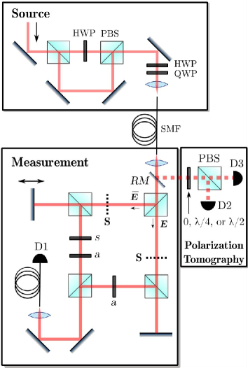
In Fig. 1 the partially polarized beam entering the MZ is
separated by a 50:50 beam splitter into primary test beam and auxiliary beam . The two beams
inherit the same statistical properties from their mother beam and
thus both can be expressed as in Eq. (11), with
corresponding intensities and . The auxiliary beam
obtains an unimportant phase from the beam splitter.
To determine the joint probability of the test beam , the first step is to project the field in the lab space to obtain . This can be realized by the polarizer labelled on the bottom arm of the MZ. The transmitted beam retains both components in function space:
| (8) |
where is the intensity, and and are normalized amplitude coefficients with . Here relates to the joint probability in an obvious way: . One sees that the intensities and can be measured directly but not the coefficient .
For our aim is to produce a field that combines a projection onto in function-space with the projection in lab space. The challenge of overcoming the lack of “polarizers” for projection of a non-deterministic field onto an arbitrary direction in its infinite-dimensional function space is managed as follows by employing the auxilliary field in the left arm Qian-Eberly . We pass it through the lab space polarizer rotated from the initial basis by a specially chosen angle , so that the statistical component is stripped off. The transmitted beam then has only the component, as desired: . Here is the corresponding intensity and the special angle is given by SupplMat ; Qian-Eberly .
The function-space-oriented beam is then sent through another polarizer to become , where is the corresponding intensity. Finally, the beams and are combined by a 50:50 beam splitter which yields the outcome beam . The total intensity of this outcome beam can be easily expressed in terms of the coefficient .
Some simple arithmetic will immediately provide the joint probability in terms of various measurable intensities:
| (9) |
Other values can be obtained similarly by rotations of polarizers and . To make measurements, polarizers are simultaneously rotated using motorized mounts, while the third polarizer is fixed at some value.
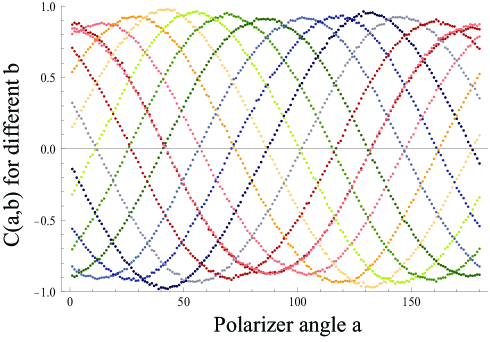
For each angle, measurements are made at detector D1 for the total intensity , and the separate intensities from each arm and by using the shutters alternately. From these measurements C(a,b) can be determined and Eq (Violation of Bell’s Inequalities with Classical Shimony-Wolf States: Theory and Experiment) is used to evaluate the CHSH parameter .
Fig. 2 shows obtained by measuring the joint probabilities for a complete rotation of polarizer , with different curves corresponding to (and thus ) fixed at different values. It is apparent from the near-identity of the curves that, to good approximation, the correlations are a function of the difference in angles, i.e. . Then the maximum value for can be found straightforwardly from any one of the curves in Fig. 2. Among them the smallest and largest values of are and .
In summary, we defined a field or state to be classical and therefore not quantum mechanical in any way, but required it to satisfy several quantum-like conditions. Its bipartite pure state form demonstrates the clear entanglement of its independent degrees of freedom. This is in common with pure two-party quantum systems. It is dynamically probabilistic, meaning that individual field measurements yield values that cannot be predicted except in an average sense, another feature shared with quantum systems but also associated for more than 50 years with well-understood and well-tested optical coherence theory Brosseau-Wolf . Such so-called Shimony-Wolf states that embody this combination of features have a range of correlation strengths that is restricted by the conditions of the CHSH Bell inequality. Experimental tests showed that the Shimony-Wolf states violate the same inequality proved for them, attaining Bell-violating levels of correlation similar to those found in tests of quantum systems brightBell .
The explanation for the CHSH inequality violation is not hard to find, but is important because it makes yet another connection between classical Shimony-Wolf states and quantum systems. We recall that hidden variables were allowed by Bell (and in the CHSH derivation) to be present and to act on the bipartite degrees of freedom, and to induce correlations between them. But so long as the observation made on one of the parts of a tested system are independent of observations made on the other part, a Bell inequality will limit those correlation strengths. But, exactly as for quantum systems, Shimony-Wolf states have an embedded structural contingency. This contingency is the entanglement of the two examined degrees of freedom. In effect, we have provided a way of examining a new sector of the boundary between quantum and classical. The violation demonstrated here shows that, in contrast to a wide understanding, Bell violation has nothing special to do with quantum mechanics, but everything to do with entanglement.
Acknowledgements The authors acknowledge helpful discussions over several years with many colleagues including A.F. Abouraddy, A. Aspect, C.J. Broadbent, L. Davidovich, E. Giacobino, G. Howland, A.N. Jordan, G. Leuchs, P.W. Milonni, R.J.C. Spreeuw, A.N. Vamivakas, as well as financial support from NSF PHY-0855701, NSF PHY-1203931, and DARPA DSO Grant No. W31P4Q-12-1-0015.
References
- (1) B.N. Simon, S. Simon, F. Gori, M. Santarsiero, R. Borghi, N. Mukunda, and R. Simon, “Nonquantum Entanglement Resolves a Basic Issue in Polarization Optics”, Phys. Rev. Lett. 104, 023901 (2010). See also M. Sanjay Kumar and R. Simon, “Characterization of Mueller matrices in polarization optics”, Opt. Commun. 88, 464 (1992), and F. Töppel, A. Aiello, C. Marquardt, E. Giacobino, and G. Leuchs, “Classical entanglement in polarization metrology”, arXiv:1401:1543 (2014).
- (2) X.F. Qian and J.H. Eberly, “Entanglement and classical polarization states”, Opt. Lett. 36, 4110 (2011). See also T. Setälä, A. Shevchenko and A. Friberg, “Degree of polarization for optical near fields”, Phys. Rev. E 66, 016615 (2002), and J. Ellis and A. Dogariu, “Optical polarimetry of random fields”, Phys. Rev. Lett. 95, 203905 (2005).
- (3) K.H. Kagalwala, G. DiGiuseppe, A.F. Abouraddy and B.E.A. Saleh, “Bell’s measure in classical optical coherence”, Nature Phot. 7, 72 (2013).
- (4) R.J.C. Spreeuw, “A Classical Analogy of Entanglement”, Found. Phys. 28, 361-374 (1998).
- (5) P. Ghose and M.K. Samal, “EPR Type Nonlocality in Classical Electrodynamics”, arXiv:quant-ph/0111119 (2001).
- (6) K.F. Lee and J.E. Thomas, “Entanglement with classical fields” Phys. Rev. Lett. 88, 097902 (2002).
- (7) C.V.S. Borges, M. Hor-Meyll, J.A.O. Huguenin, and A.Z. Khoury, “Bell-like Inequality for the spin-orbit separability of a laser beam”, Phys. Rev. A 82, 033833 (2010).
- (8) M.A. Goldin, D. Francisco and S. Ledesma, “Simulating Bell inequality violations with classical optics encoded qubits”, J. Opt. Soc. Am. 27, 779 (2010).
- (9) A. Shimony, “Contextual Hidden Variables Theories and Bell’s Inequalities”, Brit. J. Phil. Sci. 35, 25-45 (1984). See also “Bell’s Theorem”, A. Shimony, in Stanford Encycl. of Philosophy, http:/plato.stanford.edu/entries/bell-theorem (2009).
- (10) E. Wolf, “Coherence Properties of Partially Polarized Electromagnetic Radiation”, N. Cim. 13, 165 (1959).
- (11) S.J. Freedman and J.F. Clauser, “Experimental Test of Local Hidden-Variable Theories”, Phys. Rev. Lett. 28, 938 (1972).
- (12) A. Aspect, P. Grangier and G. Roger, “Experimental Realization of Einstein-Podolsky-Rosen-Bohm Gednakenexperiment: a new violation of Bell’s Inequalities”, Phys. Rev. Lett. 49, 91 (1982); and A. Aspect, J. Dalibard, and G. Roger, “Experimental Test of Bell’s Inequalities Using Time-Varying Analyzers”, Phys. Rev. Lett. 49, 1804 (1982).
- (13) Z.Y. Ou and L. Mandel, “Violation of Bells inequality and classical probability in a 2-photon correlation experiment”, Phys. Rev. Lett. 61, 50 (1988).
- (14) Y.-H. Shih and C.O. Alley, “New Type of Einstein-Podolsky-Rosen-Bohm Experiment Using Pairs of Light Quanta Produced by Optical Parametric Down Conversion”, Phys. Rev. Lett. 61, 2921 (1988).
- (15) M.A. Rowe, D. Kielpinski, V. Meyer, C.A. Sackett, W.M. Itano, C. Monroe, and D.J. Wineland, “Experimental violation of a Bell’s inequality with efficient detection”, Nature 409, 791 (2001).
- (16) See, for example, A. Ekert and P.L. Knight, “Entangled Quantum-Systems and the Schmidt Decomposition”, Am. J. Phys. 63, 415 (1995). The original paper is: E. Schmidt, “Zur Theorie der linearen und nichtlinearen Integralgleichungen. 1. Entwicklung willküriger Funktionen nach Systeme vorgeschriebener”, Math. Ann. 63, 433 (1907). The Schmidt theorem is a continuous-space version of the singular-value decomposition theorem for matrices. For background, see M.V. Fedorov and N.I. Miklin, “Schmidt modes and entanglement”, Contem. Phys. 55, 94 (2014).
- (17) The functions can be obtained as eigenfunctions of integral equations in which the kernel is a component’s individual autocorrelation function. See M. Kac and A.J.F. Siegert, “An explicit representation of a stationary gaussian process”, Ann. Math. Stat. 18 438-442 (1947), and L. Mandel and E. Wolf, “Optical Coherence and Quantum Optics”, Cambridge Univ. Press (1995), Chap. 2.
- (18) J.S. Bell, “On the Einstein Podolsky Rosen Paradox”, Physics 1, 195 (1964) and J.S. Bell, “On the problem of hidden variables in quantum mechanics”, Rev. Mod. Phys. 38, 447-452 (1966).
- (19) J.S. Bell, Speakable and Unspeakable in Quantum Mechanics (Cambridge Univ. Press, Cambridge, 2004), 2nd edition. Essays 4, 7, 16, and 24 are particularly relevant here.
- (20) J.F. Clauser, M.A. Horne, A. Shimony and R.A. Holt, “Proposed Experiment to Test Local Hidden-Variable Theories”, Phys. Rev. Lett. 23, 880 (1969).
- (21) See C. Brosseau, Fundamentals of Polarized Light: A Statistical Optics Approach (Wiley, New York, 1998) and E. Wolf, Introduction to the Theory of Coherence and Polarization of Light (Cambridge Univ. Press, 2007)
- (22) N. Gisin, “Bell’s inequality holds for all non-product states”, Phys. Lett. A 154, 201 (1991).
- (23) See supplemental material.
- (24) See X.-F. Qian and J.H. Eberly, “Entanglement is Sometimes Enough”, arXiv:1307.3772.
- (25) See Paul G. Kwiat, Klaus Mattle, Harald Weinfurter, Anton Zeilinger, Alexander V. Sergienko, and Yanhua Shih, “New High-Intensity Source of Polarization-Entangled Photon Pairs”, Phys. Rev. Lett. 75, 4337 (1995), and Paul G. Kwiat, Edo Waks, Andrew G. White, Ian Appelbaum, and Philippe H. Eberhard, “Ultrabright source of polarization-entangled photons”, Phys. Rev. A 60, R773(R) (1999).
I Supplemental Material
Polarization tomography
To measure the polarization state, polarization analysis is performed by inserting a removable mirror RM at the input of the Mach-Zehnder interferometer to send the light to a polarization tomography setup (see illustration in Fig. 1 in the Letter). Using a polarizing beam splitter and half and quarter wave plates to project onto circular and diagonal bases, the Stokes parameters are measured (normalized values given in the text) and then used for calculation of the degree of polarization (DOP) (see Brosseau-Wolf-SM ), i.e.,
| (10) |
This is then used to find the Schmidt coefficients and of the Shimony-Wolf light field:
| (11) |
According to Qian-EberlyOL-SM one finds
| (12) |
Determining the stripping angle
This section introduces in detail how a projection in the lab space works effectively as a stripping of a basis (e.g., the component ) in function space. The light beam (11) can always be rewritten in the rotated function space basis , , i.e,
| (13) | |||||
Obviously, one notes from the second term of the equation that a properly chosen polarizer that blocks completely the polarization component will effectively strip off the function space basis .
Such a stripping polarizer can be defined as a rotation of the lab space basis by an angle , i.e.,
| (14) |
Then the stripping condition is directly given as
| (15) |
Some simple arithmetic leads to the following restriction on the rotation angle :
| (16) |
which is determined by the values of and for any rotation angle .
As a result of this stripping polarizer, the beam (13) becomes
| (17) | |||||
Apparently, the function space component of the transmitted beam is completely stripped off. By comparing the first term of Eq. (13) with Eq. (17), one notes that this stripping technique passes only a fraction of the light that has the component in the function space. Therefore it cannot be immediately regarded as a projection in the function space.
CHSH inequality
In this section we provide details of the derivation of the CHSH inequality CHSH-SM for classical statistical light beams. As introduced in the Letter, a classical light field can always be decomposed into the optimum Schmidt form (11). To follow convention we name the lab space containing , as party “A”, and the statistical function space with , as party “B”.
To examine the beam (11) in lab space, one makes measurements in an arbitrary polarization-rotated basis , . We designate the measurement result in this basis as , which takes the maximum value if all the light is registered in basis , and when all the light registered in . Consequently, for the most general case when the light contains both polarization components the measurement result can be defined as
| (18) |
where with is the probability of finding the statistical light beam in lab basis . The normalization condition is satisfied. By this definition one notes that is exactly the Stokes parameter Brosseau-Wolf-SM in the corresponding basis, and it is continuously varying between and .
Similarly one can characterize the measurement of the light beam in the effective two-dimensional function space by defining an analogous measurement result as
| (19) |
where with is the probability of finding the statistical light beam in function basis , and . Note that is also bounded between and .
In general, an average measurement outcome of one space may condition on the status of the other space. Moreover, from the argument of Bell Bell64-66-SM , it could also be influenced by some unknown and/or unmentioned variables and parameters such as environmental noises, the detector conditions, or more fundamental hidden variables, etc. We follow tradition in the discussion of Bell inequality monitoring and label these so-called “contextual” classical unknowns collectively by a single multi-dimensional parameter with an overall unknown distribution . Therefore the measurement result in lab space can be rewritten by admitting all such dependences:
and similarly
Then the measurement outcome correlation between the lab and function spaces can be characterized as
| (20) |
As usual, measurement outcomes in “A” space are assumed to be independent of measurements and setups made in “B” space, and vice versa, so we have in terms of measurement results the simpler forms and . It is important to note that this assumption does not exclude possible correlations between the measurements in the two spaces, i.e., the outcomes in both spaces may still be related because of . Consequently the correlation function (20), for arbitrary angles and , is equivalent to
| (21) |
Then one can follow the standard CHSH procedure CHSH and find
| (22) | |||||
From the fact that any measurement results and lie between the values and , the expression for straightforwardly obeys the familiar inequality for any , , , . This concludes the derivation of the CHSH inequality.
References
- (1) See C. Brosseau, Fundamentals of Polarized Light: A Statistical Optics Approach (Wiley, New York, 1998) and E. Wolf, Introduction to the Theory of Coherence and Polarization of Light (Cambridge Univ. Press, 2007).
- (2) See X.F. Qian and J.H. Eberly, “Entanglement and classical polarization states”, Opt. Lett. 36, 4110 (2011).
- (3) J.F. Clauser, M.A. Horne, A. Shimony and R.A. Holt, “Proposed Experiment to Test Local Hidden-Variable Theories”, Phys. Rev. Lett. 23, 880 (1969).
- (4) J.S. Bell, “On the Einstein Podolsky Rosen Paradox”, Physics 1, 195 (1964) and J.S. Bell, “On the problem of hidden variables in quantum mechanics”, Rev. Mod. Phys. 38, 447-452 (1966).