Bulk viscosity-driven suppression of shear viscosity effects on the flow harmonics at RHIC
Abstract
The interplay between shear and bulk viscosities on the flow harmonics, ’s, at RHIC is investigated using the newly developed relativistic 2+1 hydrodynamical code v-USPhydro that includes bulk and shear viscosity effects both in the hydrodynamic evolution and also at freeze-out. While shear viscosity is known to attenuate the flow harmonics, we find that the inclusion of bulk viscosity decreases the shear viscosity-induced suppression of the flow harmonics bringing them closer to their values in ideal hydrodynamical calculations. Depending on the value of the bulk viscosity to entropy density ratio, , in the quark-gluon plasma, the bulk viscosity-driven suppression of shear viscosity effects on the flow harmonics may require a re-evaluation of the previous estimates of the shear viscosity to entropy density ratio, , of the quark-gluon plasma previously extracted by comparing hydrodynamic calculations to heavy ion data.
I Introduction
One of the the main results stemming from heavy-ion collision experiments at the Relativistic Heavy Ion Collider (RHIC) and the Large Hadron Collider (LHC) is the discovery that the Quark-Gluon Plasma (QGP) behaves as a nearly perfect fluid Gyulassy:2004zy in which the lowest value of Heinz:2013th . While there have been several model calculations that support such a small value for in the QGP Danielewicz:1984ww ; Kovtun:2004de ; Nakamura:2004sy ; Meyer:2007ic ; Xu:2007ns ; Xu:2007jv ; Hirano:2005wx ; Csernai:2006zz ; Hidaka:2008dr ; NoronhaHostler:2008ju ; NoronhaHostler:2012ug ; Ozvenchuk:2012kh , much less is known about the bulk viscosity to entropy density ratio, . In fact, though it is true that vanishes at sufficiently large temperatures Arnold:2006fz , it is not clear at the moment how large this quantity can be Meyer:2007dy ; Karsch:2007jc in the range of temperatures probed in heavy ion collisions, MeV.
This has led to the idea that the bulk viscosity may be extremely small and have negligible effects on observable quantities such as the azimuthal flow anisotropies (for phenomenological consequences of large bulk viscosity in heavy ion collisions see Torrieri:2007fb ; Rajagopal:2009yw ; Habich:2014tpa ). Most studies have used only shear viscous calculations and then fitted the calculated flow harmonics to experimental data to estimate the shear viscosity of the QGP etas . There are a few exceptions of those who have explored bulk viscosity Song:2009rh ; Bozek:2009dw ; Monnai:2009ad ; Denicol:2009am ; Denicol:2010tr ; Dusling:2011fd and its effects on elliptic flow but further work was needed to quantify the effects of bulk viscosity on the higher order flow harmonics. Recently, in Noronha-Hostler:2013gga the effects solely from bulk viscosity on the flow harmonics at RHIC were investigated using event-by-event hydrodynamics and it was found that bulk viscosity enhances the differential flow harmonics with respect to the ideal case, which is the opposite effect found in the case of shear viscosity etas .
In this paper we will explore the interplay between bulk and shear viscosities within the framework of relativistic hydrodynamical modeling using v-USPhydro Noronha-Hostler:2013gga , which is a boost invariant viscous hydrodynamical code that runs event-by-event initial conditions using Smoothed Particle Hydrodynamics (SPH) originalSPH ; SPHothers ; Aguiar:2000hw to solve the equations of motion. For some choices of the model parameters, we find that for A GeV RHIC collisions bulk viscosity can almost entirely negate the effects of shear viscosity when they are of a comparable size for both the integrated and dependent flow harmonics. In fact, in this case for differential flow harmonics bulk viscosity effects dominate over the effects from shear. However, we find that there is a strong dependence on the model choice of bulk viscous corrections at freeze-out for the differential flow harmonics at intermediate GeV (at low both methods converge and, thus, the integrated flow harmonics are much more robust with respect to model changes in the viscous contribution to the particle distributions). Finally, we find that bulk viscosity has a nontrivial effect on the shear stress tensor even when the chosen is significantly smaller than the shear viscosity.
This paper is organized as follows. In Section II we cover the relativistic hydrodynamical model that we are using. In II.1 we discuss the equations of motion for 2+1 relativistic hydrodynamics with bulk and shear viscosity using the SPH formalism then in Section II.2 we show the transport coefficients used for this paper. In Section II.3 the setup for our Glauber event-by-event initial conditions are discussed and in Section II.4 we discuss the parameters and equations for the freeze-out with viscous corrections. In Section III we explore the effects of shear and bulk viscosities on the hydrodynamical evolution while in Section IV we discuss the results of our work for both the integrated ’s in IV.1 and the differential ’s in IV.2. We also show a comparison for the case when bulk and shear viscosities have the same magnitude in Section IV.3. Finally, in Section V we discuss the consequences of our work. Details about the equations and tests of the accuracy of v-USPhydro can be found in the Appendices.
Definitions: We use a flat space-time metric in Milne coordinates defined as where and
| (1) |
are the proper time and space-time rapidity, respectively. Furthermore, we assume boost invariance for the flow velocity so and also . Natural units are employed throughout this work, i.e., .
II Details of the Hydrodynamic Model
II.1 Equations of Motion for 2+1 relativistic hydrodynamics with bulk and shear viscosities
In this paper we use a boost invariant setup with a vanishing baryon chemical potential and the conservation of energy and momentum can be written as
| (2) |
where the Christoffel symbol is
| (3) |
The general expression for energy-momentum tensor that includes both bulk and shear viscosity effects is
| (4) |
where is the bulk viscous pressure, is the shear stress tensor, and the spatial projection operator is . Above, we use the Landau definition for the local rest frame, and the remaining dynamical quantities are the energy density , the pressure (which can be written in terms of via the equation of state) and the fluid 4-velocity . The dissipative currents and obey relaxation-type differential equations and the full form of these equations, at least according to kinetic theory, can be found in Denicol:2012cn . In this paper we do not consider all the terms found in Denicol:2012cn due to the large uncertainty regarding the values of the many new transport coefficients involved (for a recent study involving the determination of these coefficients in certain limits see Denicol:2014vaa ). Rather, we use as in our previous work Noronha-Hostler:2013gga the simplest equation for the bulk scalar (obtained originally via the memory function prescription Koide:2006ef and used also in Denicol:2009am ; Denicol:2010tr )
| (5) |
where is the comoving covariant derivative, is the fluid expansion rate, and is the bulk relaxation time coefficient. For the description of the shear stress tensor we use the minimal Israel-Stewart description (compatible with conformal invariance)
| (6) |
where we defined the tensor projector , the shear tensor , and is the shear relaxation coefficient. Therefore, in this work we have 4 transport coefficients: , and their respective relaxation times and . We note that we included the term in the equations of motion for to make it possible to check the accuracy of our code against the analytical and semi-analytical solutions found in Ref. Marrochio:2013wla (shown in detail in Appendix A.2).
The fluid dynamical evolution is written using the Lagrangian approach within the Smoothed Particle Hydrodynamics (SPH). An in depth discussion of the SPH formalism and its relationship to the equations of motion can be found in Hama:2004rr ; Denicol:2009am ; Denicol:2010tr ; Noronha-Hostler:2013gga ; Noronha-Hostler:2013ria ; Andrade:2013poa .
II.2 Model choice for the transport coefficients and equation of state
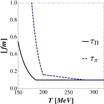
The v-USPhydro code has the ability to run ideal, bulk, shear, and shear+bulk 2+1 hydrodynamics (a generalization of the code to include full 3+1 dynamics is in the making). In this paper we consider the temperature dependent shear, bulk, and relaxation time coefficients shown in Fig. 1.
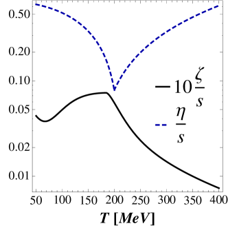
For the temperature dependent shear viscosity we use the parametrization done in Niemi:2012ry that describes the low temperature region using the result from the extended mass spectrum hadronic model NoronhaHostler:2008ju while at high temperatures is given by the lattice data of Ref. Nakamura:2004sy . It reads
| (7) |
where MeV and the shear relaxation time Denicol:2010xn ; Denicol:2011fa is taken to be
| (8) |
We have used the following bulk viscosity coefficient (inspired by Buchel’s formula Buchel:2007mf for a strongly coupled plasma)
| (9) |
with the corresponding temperature dependent bulk relaxation time, (see Huang:2010sa )
| (10) |
Given the small value of used here, we note that in Fig. 1 we actually plot in order to better illustrate its temperature dependence. Furthermore, we always ensure that and are greater than 0.1 fm (the time step size of the numerical code) to avoid stability issues.
II.3 Initial conditions
| Centrality | |
|---|---|
| 274.95 | |
| 195.98-274.95 | |
| 139.01-195.98 | |
| 96.99-139.01 | |
| 61.95-96.99 | |
| 37.04-61.95 |
In this paper we only consider Monte Carlo Glauber simulations of Au+Au collisions at RHIC at GeV ic as our initial conditions for the energy density. We begin the relativistic fluid-dynamical evolution at fm (for testing of this assumption see Noronha-Hostler:2013gga ). Our centrality classes are found by binning the results for over 15,000 events and they are well in agreement with other Monte Carlo Glauber simulations Adler:2003cb . The relationship between and the centrality classes is shown in Tab. 1. Within each centrality class we calculate 150 hydrodynamical events on an event-by-event basis.
As in our previous work using the v-USPhydro code Noronha-Hostler:2013gga , our initial energy density is
| (11) |
where is the number density of binary collisions in the event, which is fixed to obtain on average direct ’s in central (averaged ) RHIC collisions (this number of direct pions, when added to the yield coming from particle decays, leads to the correct number of ’s in this case). Also, in this paper particle decays and hadronic transport have not been taken into account. Furthermore, we assume that , , and the spatial components of vanish at .
II.4 Cooper-Frye Freeze-out
Viscous corrections enter not only in the hydrodynamical equations of motion discussed in Section II.1 but also in the distribution function for the Cooper-Frye freeze-out Cooper:1974mv . We perform the freeze-out on an isothermal hypersurface with the freeze-out temperature MeV Noronha-Hostler:2013gga . The distribution function for a given hadron is described as
| (12) |
where the ideal component of the distribution function, , is
| (13) |
where for fermions, for bosons, and for classical Boltzmann statistics. The general form of the correction term for bulk viscosity, , up to second order in powers of is Noronha-Hostler:2013gga
| (14) |
where , , and depend on the particle type (mass, degeneracy) and freeze-out temperature. In this paper we consider both the coefficients determined from the Moments Method (MOM) in Denicol:2012cn ; Denicol:2012yr ; Noronha-Hostler:2013gga and those derived by Monnai and Hirano (MH) in Monnai:2009ad . MH implemented Grad’s 14-moment method for multi-particle species to compute the bulk viscous contribution to the distribution function. MOM is based on the novel procedure proposed in Denicol:2012cn to derive viscous hydrodynamic equations from the Boltzmann equation, generalized to include the case involving different hadron species.
The exact coefficients for each method were determined in Noronha-Hostler:2013gga for the case of pions with MeV and for MOM we obtain
| (15) |
while for MH
| (16) |
Finally, we take the “democratic” Ansatz for the correction term for shear viscosity,
| (17) |
(for a recent discussion on the validity of such an Ansatz in kinetic theory see Molnar:2014fva ).
The final expression for the pion spectrum in the SPH formalism, including both shear and bulk viscosity effects, is worked out in Appendix B and we refer the reader to that section for the necessary details.
III Viscous Effects in the Hydrodynamical Evolution
 |
|
 |
 |
 |
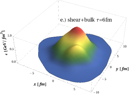 |
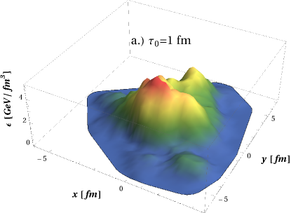
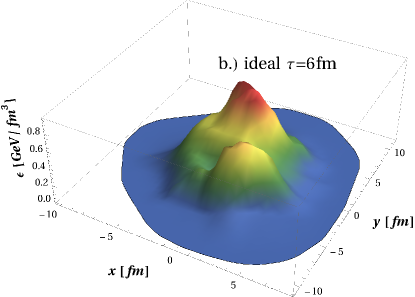
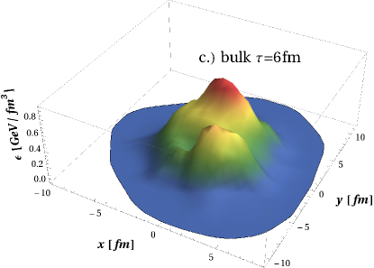
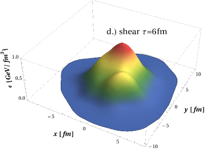
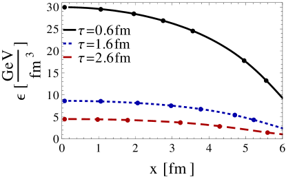
In this section we describe the interplay between shear and bulk viscosity within the fluid evolution. To do so we consider here first the effects of viscosity on the energy density over an interval of fm (we start the evolution at fm and plot the energy density profile at fm) for a random initial condition shown in Fig. 2 a.) for RHIC’s centrality class. We then include plots of the fluid evolution of the energy density at fm for b.) ideal hydrodynamics, c.) viscous hydrodynamics with only bulk viscosity, d.) viscous hydrodynamics with only shear viscosity effects, and e.) viscous hydrodynamics with both bulk and shear viscosity.
One can clearly see in Fig. 2 that there are qualitative differences between the ideal and viscous fluids. The ideal hydrodynamical evolution preserves most of the initial structure of the energy density even after fm. The bulk viscous case evolution does not maintain as many peaks and valleys at the ideal case but still displays more structure than both the shear and shear+bulk hydro events. Moreover, it is flatter than all the other events (recall that bulk viscosity acts against radial expansion). For the energy density profile we are able to see no difference between the bulk and the shear+bulk case, which indicates that the shear viscosity dominates the viscous corrections to energy density throughout the hydrodynamical evolution. This is not surprising considering that our chosen is relatively small in comparison to and the energy density is a relatively robust observable.
| 0-10% | 1.79% | 8.59% | 1.14% | -59.72% | 2.03% | 20.50% |
| 10-20% | 2.48% | 8.95% | 2.89% | -52.37% | 2.19% | 20.59% |
| 20-30% | 2.87% | 8.96% | 4.07% | -40.70% | 2.02% | 20.66% |
| 30-40% | 3.49% | 9.15% | 3.47% | -36.96% | 2.15% | 19.97% |
| 40-50% | 4.14% | 9.11% | 3.52% | -37.23% | 2.00% | 20.86% |
| 50-60% | 4.98% | 9.23% | 6.27% | -22.55% | 2.28% | 19.73% |
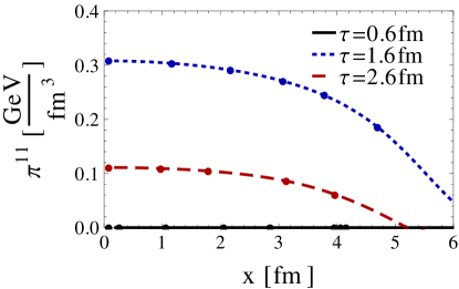
While there is little difference between the case involving only shear and shear+bulk within the energy density profile, it is interesting to see if an effect shows up in the nonzero components of the shear stress tensor and, additionally, in the bulk pressure .
To see how the inclusion of shear viscosity affects the bulk pressure, we first look at the mean (averaged over all the SPH particles) of the bulk pressure for each individual event, , and its corresponding variance and define
| (18) |
where is the mean bulk pressure of a given event with the corresponding variance when the equations of motion include both shear viscosity and bulk viscosity while is the mean bulk pressure of the same event with the corresponding variance when the equations of motion include only bulk viscosity. We then average the percentage change over all the events within each individual centrality class such that we look at the mean percentage change of the bulk pressure and the mean percentage change of the variance of the bulk pressure over all the events.
In Table 2, and takes into account the parts of the fluid that have frozen out throughout the whole time evolution, and are computed using only the parts of the fluid that have frozen out between fm and fm, and are computed using only the parts of the fluid that have frozen out in the last fm of the time evolution. In general, we see that when shear viscosity is added to our hydrodynamical evolution the changes in the bulk pressure are not large. The mean percentage change of the bulk pressure is small and only increases for more peripheral events. Also, the mean percentage change of the variance of the bulk pressure is around across all centrality classes, which means that the shear viscosity slight increases and also makes the distribution of only wider on average. The mean percentage change of and are positive and and one can see that the percentage change of the variance decreases significantly at early times while at late times it increases by for all centrality classes due to the inclusion of shear. This shows that even though the mean bulk pressure is not that affected by the presence of shear, its distribution computed event by event becomes sharper around the mean at early times and gets broadened at late times.
| Centrality | ||||
|---|---|---|---|---|
| 0-10% | -17.61% | -19.09% | -2.87% | -8.50% |
| 10-20% | -17.77% | -18.53% | -2.25% | -8.45% |
| 20-30% | -19.22% | -18.56% | -3.48% | -8.44% |
| 30-40% | -22.98% | -18.53% | -3.26% | -8.35% |
| 40-50% | -38.11% | -19.37% | -2.81% | -8.01% |
| 50-60% | -44.63% | -19.61% | -5.05% | -7.68% |
While the effects of shear on the bulk pressure are not large, the effects of bulk viscosity on the shear stress tensor are not so trivial. In Table 3 we show the percentage change in the mean values and variance of the and components of the shear stress tensor averaged over all events and all SPH particles due to the inclusion of bulk viscosity in the time evolution. These quantities are computed taking into account the parts of the fluid that have frozen out throughout the whole time evolution. We note that since is traceless, . One can see that the inclusion of bulk viscosity considerably affects : there is a suppression in its average value that increases towards more peripheral collisions while its variance also decreases by for all centralities due to the nonzero bulk viscosity. Therefore, the distribution of has a smaller mean and becomes sharper around the mean due to bulk viscosity. This occurs because bulk viscosity dampens out radial disturbances of pressure and flow, which in turn should decrease the diagonal components of the shear stress tensor. On the other hand, is only slightly affected by bulk viscosity both in terms of its mean and variance, which could be expected from symmetry arguments.
In Table 4 we show the corresponding quantities obtained from the parts of the fluid that have already frozen out after 1 fm passed the initial time . In this case, one can see that at early times the modification of the fluid velocity due to bulk viscosity has not yet affected the shear stress tensor by much. The mean value of decreases by in a way that is almost independent on centrality. This should be contrasted to the results in Table 3 which took into account the modification in this component throughout the whole time evolution due to bulk viscosity, which becomes more significant in peripheral collisions. Its variance decreases by in the most central collisions while it for peripheral collisions the suppression is . Once more, the distribution of is only slightly affected () by the presence of bulk viscosity.
| Centrality | ||||
|---|---|---|---|---|
| 0-10% | -6.66% | -12.79% | -5.94% | -10.66% |
| 10-20% | -5.32% | -11.31% | -4.87% | -9.46% |
| 20-30% | -6.07% | -12.72% | -4.81% | -9.15% |
| 30-40% | -7.01% | -14.08% | -4.80% | -9.19% |
| 40-50% | -4.75% | -9.00% | -4.75% | -8.99% |
| 50-60% | -6.83% | -15.02% | -4.63% | -8.76% |
| Centrality | ||||
|---|---|---|---|---|
| 0-10% | -17.68% | -29.13% | -5.94% | -10.80% |
| 10-20% | -15.98% | -29.09% | -4.80% | -9.38% |
| 20-30% | -15.45% | -28.56% | -4.77% | -9.06% |
| 30-40% | -14.97% | -28.28% | -4.88% | -9.34% |
| 40-50% | -13.83% | -27.91% | -4.80% | -9.20% |
| 50-60% | -12.75% | -26.18% | -4.50% | -8.51% |
At later times we see a larger effect on the shear stress tensor components from the bulk viscosity. In Table 5 we see that for almost every case both the mean and variance, regardless of centrality class, are significantly larger for late freeze-out (the last of the hydrodynamical evolution). This indicates that as the hydrodynamical evolution progresses the effects of bulk viscosity are more visible, which in the end is consistent with the results in Table 3. This occurs because it takes some time for the bulk viscosity to affect the flow and then the shear tensor and, consequently, the shear stress tensor. Furthermore, one expects that by lowering the freeze-out temperature (here we use MeV) one can increase the effects from bulk viscosity. By the same reason, going from RHIC to LHC energies one would expect that bulk viscosity becomes more relevant to the dynamical evolution of the system since at large energies the fluid stays in the QGP phase for a longer period of time.
Tables 2-5 suggest that the interplay between bulk and shear viscosities have a very non-trivial, non-linear effect on the shear stress tensor and bulk pressure already during the hydrodynamical evolution itself. While the shear only slightly increases the mean value of , the inclusion of bulk viscosity leads to a significant suppression of the shear stress tensor components. This indicates that the expected suppression of flow harmonics due to shear viscosity can be softened by the presence of bulk viscosity. In fact, in our previous work Noronha-Hostler:2013gga we suggested that it may be possible for the bulk viscosity-driven enhancement of the integrated flow harmonics ’s compensate for the expected damping of these coefficients due to shear viscosity. However, it appears that their relationship is more complicated than we initially believed.
IV Results for the Flow Harmonics
In this section we show the results for both the -integrated and the differential flow harmonics taking into account the effect of bulk and shear viscosities. We use the event plane method Poskanzer:1998yz to calculate the event plane angles ’s and a detailed explanation of the method as done in v-USPhydro can be found in Noronha-Hostler:2013gga . Additionally, in each centrality class we consider 150 events on an event-by-event basis (we have checked that the results found here are robust with respect to the inclusion of more events).
Unless stated otherwise, for the -integrated ’s we take the limits of integration to be GeV. However, due to issues previously discussed with the bulk viscous corrections within Cooper-Frye freeze-out Noronha-Hostler:2013gga , the overall viscous correction to the particle distribution at freeze-out can become larger (and negative) than the equilibrium contribution at intermediate values of (which would lead to a negative particle spectra for those values of ) if the viscous transport coefficients are large (for the coefficients shown in Fig. 1 this problem does not occur). In order to avoid such problems in the spectra and the integrated ’s when is 10 times larger than that in Eq. (9), we did not take into account the negative contribution from the corresponding part of the integral over .
IV.1 Integrated ’s
 |
 |
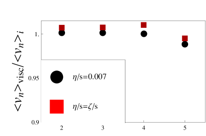
In Fig. 3 we show the ratio between the integrated ’s of direct pions at RHIC of viscous and ideal hydrodynamics across all centrality classes investigated in this paper. These quantities were computed using the moments method to determine the viscous correction to the particle distribution at freeze-out. The transport coefficients we used are defined in Section II.2. The dependence on has the steepest curve when only shear viscosity is included. The effect of bulk viscosity combined with shear viscosity slightly increases the ’s, in accordance with the conclusions found in Noronha-Hostler:2013gga that the bulk viscosity slightly increases the ’s. It is, however, a small increase since our chosen is significantly smaller than . The suppression of shear viscosity effects here occurs because, as shown in the previous section, the inclusion of bulk viscosity decreases the magnitude of the shear stress tensor components.
Finally, when one includes the effect of a “large” bulk viscosity, i.e., we see that the ’s are shifted upwards much closer to the ideal case. In this case the bulk viscosity-driven suppression of the shear stress tensor is very significant. We note here that our initial bulk viscosity is so small that even after multiplying by a factor of 10, its peak is still not as large as the minimum of the shear viscosity (see Fig. 1). Thus, we do not expect that the bulk viscosity can completely counteract shear viscous effects even in this case. Furthermore, due to above mentioned limitations in the , for the case with one can only integrate to GeV (which in any case is the integration interval that gives the major contribution to this quantity) before the spectrum becomes negative.
We note that the inclusion of bulk viscosity has the net effect to decrease the difference between and in central collisions. In fact, in the case of there is very little difference between and in the most central collisions, which is not the case towards peripheral collisions. If the bulk viscosity of the QGP is not really much smaller than , further improvements to the viscous correction involving bulk and shear are necessary for a more accurate calculation of ’s to verify the trend regarding and in central collisions found here.
 |
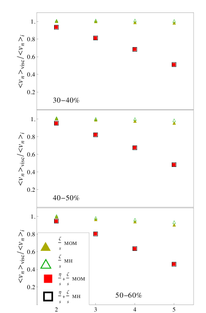 |
In Fig. 4 we compare the difference between two different choices of viscous corrections within Cooper-Frye freeze-out. As discussed in the previous section, the moments method is derived in Denicol:2012cn ; Denicol:2012yr and while MH comes from Monnai:2009ad . It appears that at least in the case of the integrated ’s there is almost no difference between the two methods for all centrality classes and ’s. The moments method shows a slight increase for the integrated ’s for both bulk and shear+bulk but the change is very small. This is because the integrated ’s are more dependent on the lower region wherein there is little difference between MOM and MH.
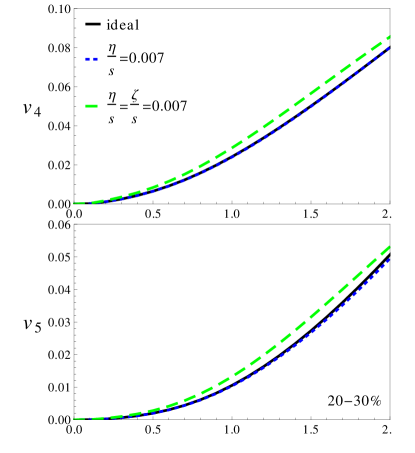
IV.2 Differential ’s
 |
 |
 |
 |
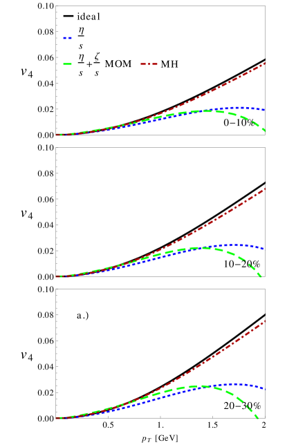 |
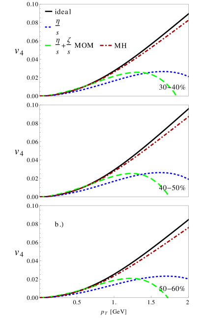 |
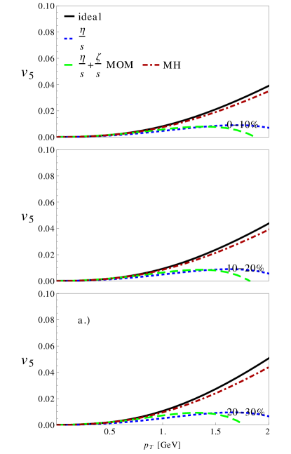 |
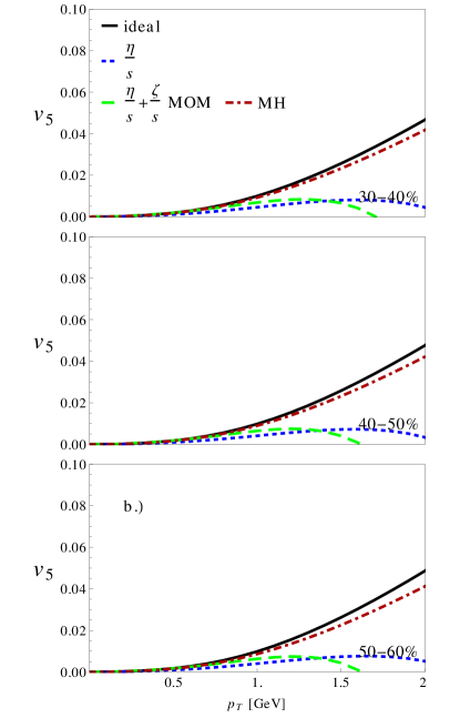 |
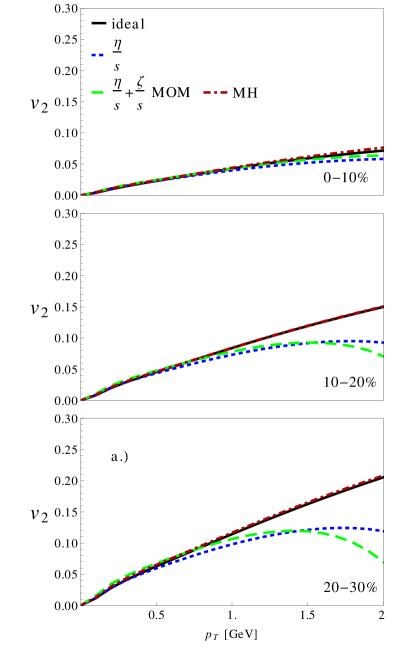
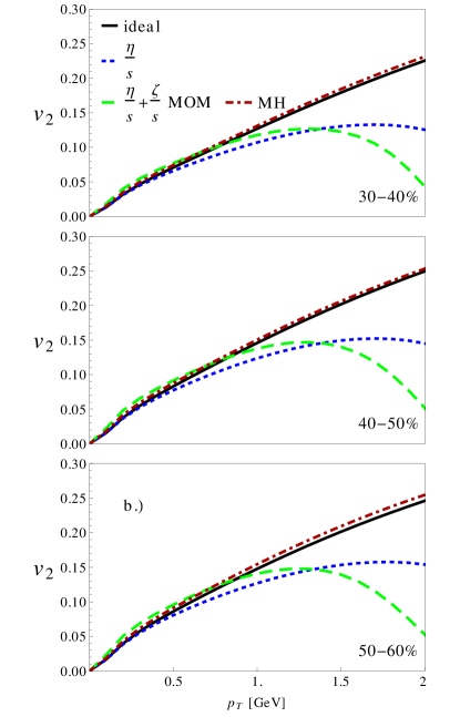
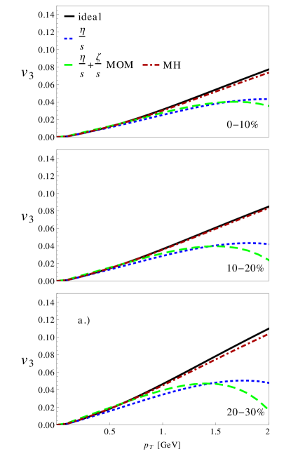
In this section we consider the dependent ’s across all centrality classes and look for the effects of bulk and shear viscosity. In Figs. 5-8 we show -, respectively. We do not include the effect of because for this large value we are only able to calculate the spectrum reliably up to GeV for MOM (in the case of MH one can integrate up to GeV). One can see that the viscous corrections considerably change the ’s, especially for large . For all the ’s and all the centralities we see a pattern: ideal hydrodynamics (solid black line) gives the largest , followed by the viscous case with shear and bulk computed using the MH formula (dark red dotted-dashed curve) and then the shear+bulk computed using the MOM expression (long-dashed green line), for which the ’s are a bit larger than the case including only shear viscosity (short-dashed blue line) for GeV. These results show that the bulk viscosity-driven suppression of shear effects also occurs for the differential flow harmonics.
In the previous section we showed that both MH and MOM give very similar integrated ’s. The same cannot be said about the differential flow harmonics. Using the MOM correction, we found that the case including effects uniformly decreases the ’s and the effect is strongest for the most peripheral collisions. Additionally, higher order ’s are more strongly affected by the combined effect of shear and bulk viscosities. We also note that for the MH curves with shear and bulk nearly match the ideal curves for all centrality classes. The same does not occur for higher order flow coefficients. In fact, as discussed in Noronha-Hostler:2013gga , the MH correction to the particle distribution diverges quickly for large . The curves computed with the MOM method start to decrease (faster than those for pure shear viscosity effects) for GeV.
IV.3 Equal Shear and Bulk viscosities
Up until this point we have always assumed that the bulk viscosity is significantly smaller than the shear viscosity. However, due to our very limited knowledge about the magnitude of in the QGP there is no a priori reason why that must be the case. While there are no limitations from the point of view of the hydrodynamic code to use larger ’s (aside from possible cavitation effects for sufficiently large ), unfortunately, due to limitations with the corrections for bulk viscosity we cannot include a bulk viscosity that is as large as the generally accepted shear viscosity . However, in order to understand what happens when both the bulk and shear viscosities have equal magnitude, we can consider a very small shear viscosity that is of the same order of magnitude as our bulk viscosity. In this section we consider the temperature independent situation where and compare to the case where only shear viscosity is included. Because the bulk viscosity generally increases the ’s (both integrated and dependent flow harmonics) and the shear viscosity generally decreases them, it is possible that when they are both of the same order of magnitude that they will reproduce the ideal results (an indication of that possibility was already found in the previous section when comparing the shear+bulk MH results for with its ideal value). Here we only look at the centrality class.
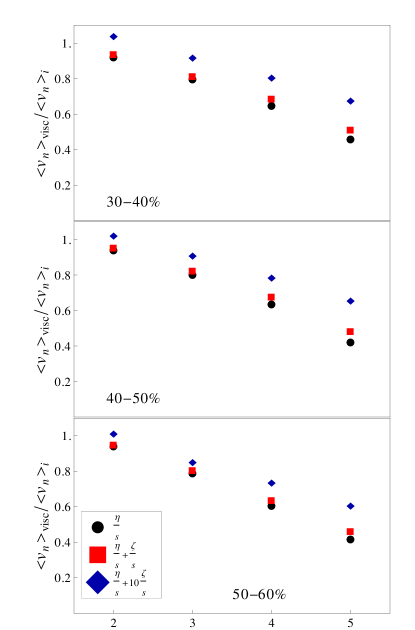
In Fig. 9 the integrated ’s for direct pions are shown for RHIC’s most central collisions. While such a small shear viscosity of has an extremely small effect on the integrated ’s, one can still see that it does decrease the ’s and the higher order ’s are most strongly affected. However, when bulk viscosity is included we see that the integrated ’s return to almost precisely the result for ideal hydrodynamics (with the exception of , which remains slightly below still). This indicates that it may be possible for bulk viscosity to compensate for the effects of shear viscosity in the integrated ’s when they are both of the same order of magnitude.
 |
 |
In Fig. 10 we observe the dependent flow harmonics of direct pions in the centrality class for the small case. One can see that there is no visible difference between the ideal case and that of a small shear viscosity of . However, when the bulk and shear viscosities are identical the dependent ’s increase, which indicates that the effect of bulk viscosity dominates the dependent ’s when bulk and shear are of the same order of magnitude. This was hinted already in Fig. 3 when we used . However, in that case we were limited to a small range over which we could integrate our spectrum due to the problems of the . Here we avoid that problem due to the small value of and .
V Conclusions
In this paper we used v-USPhydro (a 2+1 Lagrangian hydrodynamical model) to study the effects of both bulk and shear viscosities on the hydrodynamical evolution of the QGP and the resulting anisotropic collective flow harmonics at RHIC. We found that even though in our equations of motion the shear stress tensor and the bulk scalar do not couple directly, their indirect coupling via the flow velocity is still strong enough for them to influence each other in a nonlinear fashion. We found that the inclusion of even a small bulk viscosity decreases the well-known shear viscosity-induced suppression of both the integrated and differential flow harmonics bringing them closer to their values in ideal hydrodynamical calculations. This is a new effect brought in by bulk viscosity in event by event hydrodynamic simulations.
Furthermore, we found that when the bulk and shear viscosities are roughly the same order of magnitude the bulk viscosity negates a significant portion of the contribution from shear viscosity for the integrated flow harmonics. In fact, for the differential flow harmonics the bulk viscosity dominates and actually increases the flow harmonics, which is the opposite effect when only the shear viscosity is considered. Even if one considers only a small we find that the bulk viscosity tempers the suppression typically demonstrated from the shear viscosity. When one looks only at the relativistic hydrodynamical expansion one can clearly see that the presence of bulk viscosity suppresses the components of the shear stress tensor. Additionally, we find that this effect plays the largest role the longer the system is expanding. Thus, for the case of lower freeze-out temperatures and also for higher collision energies where one expects to see more time spent within the hydrodynamical expansion, one would expect that the effects of bulk viscosity are more relevant.
The effects of viscosity are most relevant for peripheral collisions and higher order flow harmonics for both the integrated and differential ’s. Furthermore, we find that for the integrated ’s when we include a large that for the most central collisions but that is more significantly suppressed for more peripheral collisions. When (but both are small) basically returns to its value in ideal hydrodynamics while the same is not true for . This could indicate that the higher order flow harmonics may be vital in helping us estimate and within relativistic heavy ion collisions because they do not allow for a complete compensation of shear viscosity effects due to bulk viscosity.
Our calculations need to be improved in a number of ways. First, in this paper we did not look into the flow harmonics of hadronic species other than pions and no particle decays or hadronic afterburner effects have been included. Clearly, this must be improved to allow for a comparison to data and adequately evaluate the role played by bulk viscosity in the flow harmonics of the QGP formed in heavy ions collisions. Also, different set of initial conditions (we have only used MC Glauber in this paper) and different collisions systems and energies should be investigated. Furthermore, the considerable difference found in the differential anisotropic flow coefficients computed using two different ’s formulas is an issue that should serve as a motivation for finding a better behaved expression for the species dependent viscous corrections at freeze-out including both bulk and shear effects. Moreover, as discussed in Dumitru:2007qr , constraints on the entropy production generate a correlation between the values of transport coefficients and the initial time for hydrodynamics. If bulk viscosity effects compensate the effects from shear, could be larger than used here and, consequently, may actually be larger than usually considered in hydrodynamic simulations.
As mentioned above, the bulk viscosity-driven suppression of the shear stress tensor found here occurs in a very indirect way mediated by the modification of the flow velocity due to bulk viscosity. Indeed, in our equations of motion we do not include the known terms Denicol:2012cn which display a direct coupling between and . It would be interesting to see if the effect discussed here remains when the more general equations of motion of Denicol:2012cn and transport coefficients Denicol:2014vaa are used in the hydrodynamical evolution. We hope to address this question in the near future comment .
We remark that the actual magnitude (and temperature dependence) of in heavy ion collisions is largely unknown and it is conceivable that depending on the value of in the QGP, the bulk viscosity-driven suppression of shear viscosity effects on the flow harmonics found here may require a re-evaluation of the previous estimates of extracted from comparisons of hydrodynamic calculations (which did not include bulk viscosity effects) to heavy ion data.
Acknowledgements
We thank G. S. Denicol for helping us with the implementation of shear viscosity effects in the v-USPhydro code. We thank G. Torrieri for insightful discussions about the effects of bulk viscosity in heavy ion collisions and A. Dumitru for comments about the thermalization time and the values of transport coefficients. This work was supported by Fundação de Amparo à Pesquisa do Estado de São Paulo (FAPESP) and Conselho Nacional de Desenvolvimento Científico e Tecnológico (CNPq). This work was also financially supported by the Helmholtz International Center for FAIR within the (Landesoffensive zur Entwicklung Wissenschaftlich-konomischer Exzellenz) launched by the State of Hesse.
Appendix A Tests of the numerical code
Because of the complexity of viscous relativistic hydrodynamical equations, it is vital to test the accuracy of our numerical code. Fortunately, there are now well-known numerical and semi-analytical solutions for this purpose.
A.1 TECHQM
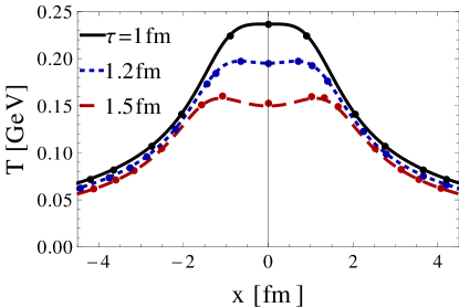
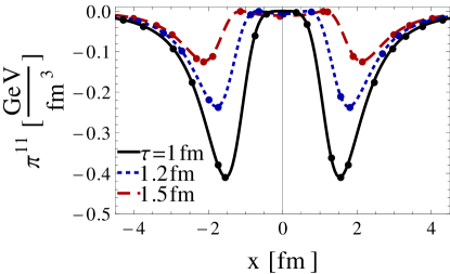
One aspect of TECHQM bulk evolution working group techqm was to ensure the overall accuracy of relativistic hydrodynamical codes and solutions for both ideal and viscous hydro evolution (with only shear viscosity) have become available. We use an ideal equation of state and the fm central Au-Au optical Glauber initial condition at RHIC A GeV. We take the starting time for hydrodynamics to be fm, , , and the freeze-out temperature is MeV. In Fig. 11 we compare our results (dots) to the TECHQM results (lines) techqm over time (solid black lines), (blue short dashed lines), and fm (red long dashed lines). One can clearly see that the results match well for multiple time steps. In our code we used the SPH smoothing parameter is fm, the total number of SPH particles is , and the time step fm.
 |
 |
|
 |
A.2 Test of Conformal Israel-Stewart Dynamics
Using symmetry arguments, Gubser Gubser:2010ze found analytical solutions of ideal and Navier-Stokes conformal hydrodynamics that are invariant under (a subgroup of ). The symmetries imply that the solution is radially symmetric in the transverse plane and boost invariant with the flow
| (19) |
where is a free parameter with dimensions of energy. This approach has been used in Marrochio:2013wla to find the first analytical and semi-analytical solutions of conformal Israel-Stewart hydrodynamics which includes nontrivial dynamics in the transverse plane. These solutions are described in detail in Marrochio:2013wla and they provide a very stringent test of the accuracy of viscous hydrodynamic codes. Since the equations of motion involving shear viscosity used here have the same structure as those in Marrochio:2013wla , we can directly test the accuracy of v-USPhydro in this case. We also note that novel analytical solutions of conformal Israel-Stewart hydrodynamics with full 3+1 dynamics can be found in Hatta:2014gqa ; Hatta:2014gga .
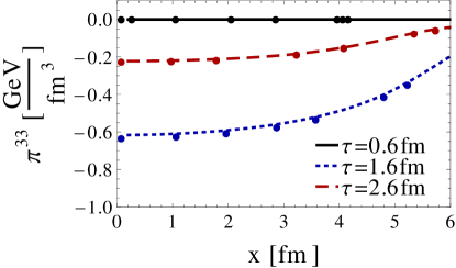
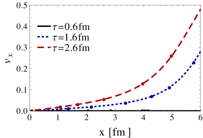
Here we compare the results from v-USPhydro to the semi-analytical solution Marrochio:2013wla in the case where , , and fm-1. The comparison involving the temperature, the flow, and a few components of the shear stress tensor can be found in Fig. 12. For our comparison we used , fm, fm, and the total number of SPH particles is . We see that v-USPhydro is able to match the semi-analytical solution pretty well at early times (the agreement remains at later times).
 |
 |
|
 |
Appendix B Details of the Cooper-Frye freeze-out in the SPH formalism
Our distribution function for a single particle species that includes effects from both shear and bulk viscosity is
| (20) |
where is the particle on-shell momentum. The ideal distribution, , is defined as
| (21) |
where for fermions, for bosons, and for classical Boltzmann statistics. For the ideal component we have
| (22) |
whereas
| (23) |
and
| (24) |
In Cartesian coordinates the scalar product of the particle momentum and the hypersurface normal vector (see Appendix C), , is
| (25) |
switching to hyperbolic coordinates
| (26) | |||||
| (27) | |||||
| (28) |
In the SPH formalism the integral over the isothermal hypersurface is written in terms of a sum of SPH particles as
| (29) |
where is the total number of SPH particles, is the normal vector of the isothermal hypersurface reconstructed using the -th SPH particle, is the 4-velocity of the SPH particle, is the bulk viscosity of the SPH particle, there is an integral over the space-time rapidity of each SPH particle , and is the shear stress tensor of the SPH particle.
Then, the contribution from a SPH particle to the ideal distribution function is
| (30) |
Substituting this into Eq. (24), we find
| (31) |
where .
The integral over the isothermal hypersurface becomes
| (32) | |||||
where we can then substitute in
| (33) |
such that
| (35) |
where
We can now insert the distribution function in Eq. (31)
but we already know a portion of this from the combination of the ideal and bulk in Noronha-Hostler:2013gga , which we will refer to here as and , so
B.1 Details about for shear
The correction term from shear viscosity effects for a given particle species is
| (39) |
where is the entropy density at freeze-out.
Using the properties of the shear stress tensor we find, in explicit form,
| (40) |
Substituting that expression in the shear correction term, one obtains for each SPH particle
After some manipulations, our final equations become
where is the modified Bessel function.
Appendix C Normal vector of isothermal surface and the SPH formalism
The normalized normal vector to the isothermal surface is
| (43) |
Since in the SPH method the spatial gradients of the pressure are known Hama:2004rr and, using the Gibbs-Duhem relation , we just need to determine to obtain . Using that , hence , and the energy conservation equation
| (44) |
we find that
| (45) |
and thus
| (46) |
Both and are still relatively small in all of our calculations, which means that the contributions from the bulk pressure and shear stress tensor in Eq. (46) are still in general very small compared to that from the energy density and pressure ( whereas the components of and ). This then means that the primary contribution to the uncorrected flow harmonics comes from the viscous corrected flow and not from the details of the freeze-out hypersurface (which remains very similar to the one found in the ideal hydro case).
References
- (1) M. Gyulassy and L. McLerran, Nucl. Phys. A 750, 30 (2005) [nucl-th/0405013].
- (2) U. Heinz and R. Snellings, Ann. Rev. Nucl. Part. Sci. 63, 123 (2013) [arXiv:1301.2826 [nucl-th]].
- (3) P. Danielewicz and M. Gyulassy, Phys. Rev. D 31, 53 (1985).
- (4) P. K. Kovtun, D. T. Son and A. O. Starinets, Phys. Rev. Lett. 94, 111601 (2005) [hep-th/0405231].
- (5) A. Nakamura and S. Sakai, Phys. Rev. Lett. 94, 072305 (2005) [hep-lat/0406009].
- (6) H. B. Meyer, Phys. Rev. D 76, 101701 (2007) [arXiv:0704.1801 [hep-lat]].
- (7) T. Hirano and M. Gyulassy, Nucl. Phys. A 769, 71 (2006) [nucl-th/0506049].
- (8) L. P. Csernai, J. .I. Kapusta and L. D. McLerran, Phys. Rev. Lett. 97, 152303 (2006) [nucl-th/0604032].
- (9) Z. Xu and C. Greiner, Phys. Rev. Lett. 100, 172301 (2008) [arXiv:0710.5719 [nucl-th]].
- (10) Z. Xu, C. Greiner and H. Stocker, Phys. Rev. Lett. 101, 082302 (2008) [arXiv:0711.0961 [nucl-th]].
- (11) Y. Hidaka and R. D. Pisarski, Phys. Rev. D 78, 071501 (2008) [arXiv:0803.0453 [hep-ph]].
- (12) J. Noronha-Hostler, J. Noronha and C. Greiner, Phys. Rev. Lett. 103, 172302 (2009) [arXiv:0811.1571 [nucl-th]].
- (13) J. Noronha-Hostler, J. Noronha and C. Greiner, Phys. Rev. C 86, 024913 (2012) [arXiv:1206.5138 [nucl-th]].
- (14) V. Ozvenchuk, O. Linnyk, M. I. Gorenstein, E. L. Bratkovskaya and W. Cassing, Phys. Rev. C 87, no. 6, 064903 (2013) [arXiv:1212.5393].
- (15) P. B. Arnold, C. Dogan and G. D. Moore, Phys. Rev. D 74, 085021 (2006) [hep-ph/0608012].
- (16) H. B. Meyer, Phys. Rev. Lett. 100, 162001 (2008) [arXiv:0710.3717 [hep-lat]].
- (17) F. Karsch, D. Kharzeev and K. Tuchin, Phys. Lett. B 663, 217 (2008) [arXiv:0711.0914 [hep-ph]].
- (18) G. Torrieri, B. Tomasik and I. Mishustin, Phys. Rev. C 77, 034903 (2008) [arXiv:0707.4405 [nucl-th]], G. Torrieri and I. Mishustin, Phys. Rev. C 78, 021901 (2008) [arXiv:0805.0442 [hep-ph]].
- (19) K. Rajagopal and N. Tripuraneni, JHEP 1003, 018 (2010) [arXiv:0908.1785 [hep-ph]].
- (20) M. Habich and P. Romatschke, arXiv:1405.1978 [hep-ph].
- (21) P. Romatschke and U. Romatschke, Phys. Rev. Lett. 99, 172301 (2007); M. Luzum and P. Romatschke, Phys. Rev. C 78, 034915 (2008) [Erratum-ibid. C 79, 039903 (2009)] [arXiv:0804.4015 [nucl-th]]; H. Song, S. A. Bass, U. Heinz, T. Hirano and C. Shen, Phys. Rev. Lett. 106, 192301 (2011) [Erratum-ibid. 109, 139904 (2012)] [arXiv:1011.2783 [nucl-th]]; H. Song, S. A. Bass and U. Heinz, Phys. Rev. C 83, 054912 (2011) [Erratum-ibid. C 87, 019902 (2013)] [arXiv:1103.2380 [nucl-th]]; H. Niemi, G. S. Denicol, P. Huovinen, E. Molnar and D. H. Rischke, Phys. Rev. Lett. 106, 212302 (2011); C. Gale, S. Jeon, B. Schenke, P. Tribedy and R. Venugopalan, Phys. Rev. Lett. 110, 012302 (2013) [arXiv:1209.6330 [nucl-th]]; B. Schenke, S. Jeon and C. Gale, Phys. Rev. Lett. 106, 042301 (2011) [arXiv:1009.3244 [hep-ph]].
- (22) H. Song and U. WHeinz, Phys. Rev. C 81, 024905 (2010) [arXiv:0909.1549 [nucl-th]].
- (23) P. Bozek, Phys. Rev. C 81, 034909 (2010) [arXiv:0911.2397 [nucl-th]].
- (24) A. Monnai, T. Hirano, Phys. Rev. C 80, 054906 (2009).
- (25) G. S. Denicol, T. Kodama, T. Koide and P. .Mota, Phys. Rev. C 80, 064901 (2009) [arXiv:0903.3595 [hep-ph]].
- (26) G. S. Denicol, T. Kodama and T. Koide, J. Phys. G 37, 094040 (2010) [arXiv:1002.2394 [nucl-th]].
- (27) K. Dusling and T. Schäfer, Phys. Rev. C 85, 044909 (2012) [arXiv:1109.5181 [hep-ph]].
- (28) J. Noronha-Hostler, G. S. Denicol, J. Noronha, R. P. G. Andrade and F. Grassi, Phys. Rev. C 88, 044916 (2013) [arXiv:1305.1981 [nucl-th]].
- (29) L. B. Lucy, ApJ. 82, 1013 (1977); R. A. Gingold and J. J. Monaghan, MNRAS 181, 375 (1977); R. A. Gingold and J. J. Monaghan, Mon. Not. Roy. Astron. Soc. 181, 375 (1977).
- (30) J. J. Monaghan, Annu. Rev. Astron. Astrophys. 30, 543 (1992); E. Chow and J. J. Monaghan, J. Comput. Phys. 134, 296 (1997); P. Laguna, W. A. Miller and W. H. Zurek, Phys. Rev. D 41, 451 (1990); R. J. Thacker, E. R. Tittley, F. R. Pearce, H. M. P. Couchman and P. A. Thomas, Mon. Not. Roy. Astron. Soc. 319, 619 (2000).
- (31) C. E. Aguiar, T. Kodama, T. Osada and Y. Hama, J. Phys. G 27, 75 (2001).
- (32) G. S. Denicol, H. Niemi, E. Molnar and D. H. Rischke, Phys. Rev. D 85, 114047 (2012).
- (33) G. S. Denicol, S. Jeon and C. Gale, arXiv:1403.0962 [nucl-th].
- (34) T. Koide, G. S. Denicol, P. .Mota and T. Kodama, Phys. Rev. C 75, 034909 (2007) [hep-ph/0609117].
- (35) H. Marrochio, J. Noronha, G. S. Denicol, M. Luzum, S. Jeon and C. Gale, arXiv:1307.6130 [nucl-th].
- (36) Y. Hama, T. Kodama and O. Socolowski, Jr., Braz. J. Phys. 35, 24 (2005) [hep-ph/0407264].
- (37) J. Noronha-Hostler, J. Noronha, G. S. Denicol, R. P. G. Andrade, F. Grassi and C. Greiner, Phys. Rev. C 89, 054904 (2014).
- (38) R. P. G. Andrade and J. Noronha, Phys. Rev. C 88, no. 3, 034909 (2013) [arXiv:1305.3098 [nucl-th]].
- (39) H. Niemi, G. S. Denicol, P. Huovinen, E. Molnar and D. H. Rischke, Phys. Rev. C 86, 014909 (2012) [arXiv:1203.2452 [nucl-th]].
- (40) G. S. Denicol, T. Koide and D. H. Rischke, Phys. Rev. Lett. 105, 162501 (2010) [arXiv:1004.5013 [nucl-th]].
- (41) G. S. Denicol, J. Noronha, H. Niemi and D. H. Rischke, Phys. Rev. D 83, 074019 (2011) [arXiv:1102.4780 [hep-th]].
- (42) A. Buchel, Phys. Lett. B 663, 286 (2008).
- (43) X. -G. Huang, T. Kodama, T. Koide and D. H. Rischke, Phys. Rev. C 83, 024906 (2011).
- (44) H. -J. Drescher and Y. Nara, Phys. Rev. C 75, 034905 (2007); Phys. Rev. C 76, 041903 (2007).
- (45) S. S. Adler et al. [PHENIX Collaboration], Phys. Rev. C 69, 034909 (2004).
- (46) F. Cooper and G. Frye, Phys. Rev. D 10, 186 (1974).
- (47) G. S. Denicol and H. Niemi, Nucl. Phys. A 904-905, 369c (2013).
- (48) D. Molnar and Z. Wolff, arXiv:1404.7850 [nucl-th].
- (49) A. M. Poskanzer and S. A. Voloshin, Phys. Rev. C 58, 1671 (1998).
- (50) A. Dumitru, E. Molnar and Y. Nara, Phys. Rev. C 76, 024910 (2007).
- (51) Recent calculations at LHC energies presented at QM2014 by the McGill group using the MUSIC 2.0 code, which includes the direct coupling between and at the level of the equations of motion, find that for ultracentral collisions the integrated and become comparable due to bulk viscosity and also other effects related to the initial conditions.
- (52) More information about this test can be found at https://wiki.bnl.gov/TECHQM/index.php/Code_checking_list.
- (53) S. S. Gubser, Phys. Rev. D 82, 085027 (2010) [arXiv:1006.0006 [hep-th]].
- (54) Y. Hatta, J. Noronha and B. -W. Xiao, Phys. Rev. D 89, 051702 (2014) [arXiv:1401.6248 [hep-th]].
- (55) Y. Hatta, J. Noronha and B. -W. Xiao, arXiv:1403.7693 [hep-th], to appear in Physical Review D.