Joint likelihood function of cluster counts and $n$-point correlation functions: Improving their power through including halo sample variance

Abstract

Naive estimates of the statistics of large scale structure and weak lensing power spectrum measurements that include only Gaussian errors exaggerate their scientific impact. Non-linear evolution and finite volume effects are both significant sources of non-Gaussian covariance that reduce the ability of power spectrum measurements to constrain cosmological parameters. Using a halo model formalism, we derive an intuitive understanding of the various contributions to the covariance and show that our analytical treatment agrees with simulations. This approach enables an approximate derivation of a joint likelihood for the cluster number counts, the weak lensing power spectrum and the bispectrum. We show that this likelihood is a good description of the ray-tracing simulation. Since all of these observables are sensitive to the same finite volume effects and contain information about the non-linear evolution, a combined analysis recovers much of the “lost” information and obviates the non-Gaussian covariance. For upcoming weak lensing surveys, we estimate that a joint analysis of power spectrum, number counts and bispectrum will produce an improvement of about $30-40\%$ in determinations of the matter density and the scalar amplitude. This improvement is equivalent to doubling the survey area.

I Introduction

Understanding the nature of dark energy is the aim of many ongoing and upcoming galaxy surveys such as the Baryon Oscillation Spectroscopic Survey (BOSS), the Kilo-Degree Survey (KiDS), the Extended BOSS (eBOSS), the Dark Energy Survey (DES) The Dark Energy Survey Collaboration (2005), the Subaru Hyper Suprime-Cam (HSC) survey Miyazaki et al. (2006), the Subaru Prime Focus Spectrograph (PFS)Takada et al. (2012), the Dark Energy Spectroscopic Instrument (DESI), the Large Synoptic Survey Telescope (LSST) LSST Science Collaboration et al. (2009), the ESA satellite mission Euclid Laureijs et al. (2011), and the NASA satellite mission WFIRST Spergel et al. (2013).

The science yield from these surveys appears to be less than one would naively expect. If we were observing a density field in the linear regime, the various modes would be uncorrelated and the amount of information available would scale with the number of modes. However, for weak lensing, the scales of interest ($l\sim 10^{3}$) are well into the non-linear regime Jain and Seljak (1997); Jain et al. (2000). On such scales, mode couplings induce non-Gaussian features, which move information from the power spectrum to the bispectrum and higher $n$-point correlation functions, and induce extra correlated scatter on the various $n$-point functions, as well as on their various multipoles Scoccimarro et al. (1999a); Hu and White (2001); Cooray and Hu (2001); Takada and Jain (2004, 2009). In order to recover the information diluted between the various multipoles and $n$-point correlation functions, one has to combine them in a joint analysis, and doing so requires an understanding of their non-Gaussian correlated errors Takada and Jain (2004); Kayo et al. (2012); Kayo and Takada (2013).

Another important source of correlated scatter comes from a finite-volume effect of the survey domain: density modes with wavelengths larger than the volume are not measurable from within the survey, but affect the observables in a predictable way Hamilton et al. (2006); Hu and Kravtsov (2003); Sefusatti et al. (2006); Takada and Bridle (2007); Takada and Jain (2009); Sato et al. (2009); Kayo et al. (2012); Takada and Hu (2013); Takada and Spergel (2013); Li et al. (2014). This is another reason to combine various observables on the same survey: since they are all affected by the same long wavelength modes, a combined analysis can determine the amplitude of these non-directly observable modes Takada and Bridle (2007); Kayo et al. (2012); Takada and Spergel (2013).

In other words, recovering the non-Gaussian information and calibrating out the long wavelength modes inaccessible from within the survey are two reasons to combine probes, and therefore justify the need for understanding their covariances. Although the first effect has been understood for a long time, progress on the second one is only recent. In Ref. Takada and Hu (2013), this ‘super-sample covariance’ in power spectrum measurement is described in terms of mode coupling through the window function and a ‘trispectrum consistency relation’. In Ref. Takada and Spergel (2013), this ‘halo sample variance’ is a consequence of the halo model: an upscatter in the average density triggers an upscatter in halo counts through linear biasing, which leads to a coherent upscatter in the various $n$-point correlation functions.

Our results derive straightforwardly from the same assumptions as the halo model: the matter overdensity field can be expressed by the distribution of halos in different mass bins, and the halos form a biased Poisson sampling of the underlying density field. The halo sample variance should therefore be considered a standard prediction of the halo model, just as much as usual decomposition $P=P^{1h}+P^{2h}$ for the power spectrum.

Our study builds on Ref. Takada and Spergel (2013) and generalizes the results therein to all $n$-point correlation functions. The starting point of our analysis is the expression of the matter overdensity in terms of halos, instead of the decomposition $P=P^{1h}+P^{2h}$, which allows for a consistent derivation of the auto- and cross-covariances between halo number counts and $n$-point functions.

The outline of this paper is the following. In Section II, we present our assumptions and derive the general formula for the halo sample variance contributions. We apply these results to the cluster counts and the matter $n$-point correlation functions in Section III. Then we apply the formulation to the 2D fields, the angular number counts of clusters and the lensing convergence $n$-point correlation functions in Section IV, which allows us to check our results against ray-tracing simulations from Ref. Sato et al. (2009). In Section V, we present an approximate joint likelihood for the cluster counts and lensing convergence power spectrum and bispectrum. We compare it to simulations and use it to forecast an estimation of cosmological parameters obtained when combining the cluster counts to the lensing power spectrum and bispectrum for a future galaxy survey.

II Method

In this section, we briefly review the halo model ingredients that we shall use to derive the halo sample variance. We present our notations and method to take into account the effects of a finite-volume survey, and give the general derivation for the halo sample variance for any observable.

II.1 Standard halo model

The halo model Seljak (2000); Peacock and Smith (2000); Ma and Fry (2000); Cooray and Sheth (2002); Hu and Kravtsov (2003) is based on the assumption that all matter in the universe is contained in halos of some mass scale. The mass function $dn/dm$ gives the mean number density for halos of mass $m$, and the density profile of halos $u_{m}(\vec{x})$, defined so as to satisfy the normalization condition $\int\!{\rm d}^{3}\vec{x}\,u_{m}(\vec{x})=1$, is assumed to depend only on their mass $m$, at a given redshift. Thus the halo model expresses the observed matter overdensity as the familiar sum over halos:

$$\hat{\delta}(\vec{k})=\int dm\left(\frac{m}{\bar{\rho}}\right)u_{m}(\vec{k})\frac{dn}{dm}\hat{\delta}^{h}_{m}(\vec{k}),$$ (1)

where $\hat{\delta}^{h}_{m}(\vec{k})$ is the number density fluctuation field (its Fourier transform) for halos of mass $m$. In what follows, we shall replace the integral with a sum over mass bins $i$, with mean mass $m_{i}$ and bin width $\Delta m_{i}$:

$$\hat{\delta}(\vec{k})=\sum_{i}\left(\frac{m_{i}}{\bar{\rho}}\right)u_{i}(\vec{k})\,\hat{n}_{i}(\vec{k},\delta_{b}).$$ (2)

Here $\hat{n}_{i}(\vec{k})$ is the halo number density field, defined as

$$\hat{n}_{i}(\vec{x})=\left.\frac{dn}{dm}\right|_{m_{i}}\Delta m_{i}\left[1+\hat{\delta}^{h}_{i}(\vec{x})\right].$$ (3)

The observed number of halos in the $i$-th mass bin $m_{i}$, for a given small volume $\delta V$ around the position $\vec{x}$, is simply given as $\hat{n}_{i}(\vec{x})\delta V$. The halo model formulation above is useful for our purpose. First, Eq. (2) shows that the statistical properties of the matter density field $\hat{\delta}(\vec{k})$ are determined by the halo number density field $\hat{n}_{i}(\vec{k})$ and the halo mass profile $u_{i}(\vec{k})$. Second, Eq. (2) allows us to straightforwardly compute cross-correlations between matter $n$-point functions and the number counts of halos as we will show below.

We assume that the halo number density in a volume element $\delta V$ around the position $\vec{x}$ follows a Poisson statistics, with mean determined by the underlying density field ${\rho_{\text{lin}}}(\vec{x})$:

$$\left\langle\hat{n}_{i}(\vec{x}_{1})\hat{n}_{j}(\vec{x}_{2})\right\rangle_{\text{Pois.}|{\rho_{\text{lin}}}} =n_{i}(\vec{x}_{1})n_{j}(\vec{x}_{2})+\delta^{K}_{ij}\delta_{D}(\vec{x}_{1}-\vec{x}_{2})n_{i}(\vec{x}),$$ (4)

where $n_{i}(\vec{x})$ is the mean halo number density for the volume $\delta V$ around $\vec{x}$, for a fixed ${\rho_{\text{lin}}}(\vec{x})$, defined as $n_{i}(\vec{x})\equiv\left\langle\hat{n}_{i}(\vec{x})\right\rangle_{\text{Pois.}|{\rho_{\text{lin}}}}$, and $\delta^{K}_{ij}$ is the Kronecker delta function: $\delta^{K}_{ij}=1$ if $i=j$, otherwise $\delta^{K}_{ij}=0$. We have assumed that the halo number densities of different mass bins are independent. We assume that the halo number densities are given as biased tracers of the linear density field ${\rho_{\text{lin}}}(\vec{x})$:

$$n_{i}(\vec{k})=\bar{n}_{i}\,b_{i}\,\delta_{\text{lin}}(\vec{k})=\left.\frac{dn}{dm}\right|_{m_{i}}\Delta m_{i}\,b_{i}\,\delta_{\text{lin}}(\vec{k}),$$ (5)

were $\bar{n}_{i}\equiv\left\langle n_{i}\right\rangle_{\rho_{\text{lin}}}\equiv\left\langle\hat{n}_{i}(\vec{x})\right\rangle_{\text{Pois.},{\rho_{\text{lin}}}}=\left.dn/dm\right|_{m_{i}}\Delta m_{i}$ is the ensemble average of the halo number density, obtained by marginalizing over Poisson sampling and different realizations of the linear density field ${\rho_{\text{lin}}}(\vec{x})$, and $b_{i}$ is the linear bias for halos of the $i$-th mass bin, $b_{i}\equiv b(m_{i})$.

Using the matter density field $\hat{\delta}(\vec{k})$ in Eq. (2), and the properties (4) and (5), it is straightforward to express the matter power spectrum $\left\langle\hat{\delta}(\vec{k})\hat{\delta}(\vec{k}^{\prime})\right\rangle$ in terms of the halo number counts:

$$\left\langle\hat{\delta}(\vec{k})\hat{\delta}(\vec{k}^{\prime})\right\rangle =\left(2\pi\right)^{3}\delta_{D}(\vec{k}+\vec{k}^{\prime})\left[\sum_{i}\left(\frac{m_{i}}{\bar{\rho}}\right)^{2}\bar{n}_{i}|u_{i}(k)|^{2}+\sum_{i,j}\left(\frac{m_{i}m_{j}}{\bar{\rho}^{2}}\right)\bar{n}_{i}\bar{n}_{j}u_{i}(k)u_{j}(k)\,\,b_{i}b_{j}P_{\text{lin}}(k)\right],$$ (6)

where $P_{\text{lin}}$ is the linear matter power spectrum. The first term is the 1-halo term, $P^{1h}(k)$, arising from correlations between matter in the same halo, while the second term is the 2-halo term, $P^{2h}(k)$, arising from matter in two different halos.

II.2 Finite survey effect: method

In this paper, we study the finite-volume effect of a survey on $n$-point correlation function measurements. We characterize the survey by its three-dimensional volume, $V_{S}$, and the average density contrast across the survey region, $\delta_{b}$. The super-survey mode is defined as $\delta_{b}\equiv\int\!d^{3}\vec{x}\,W^{3D}(\vec{x})\hat{\delta}(\vec{x})$, where $W^{3D}(\vec{x})$ is the survey window function; $W^{3D}(\vec{x})=1/V_{S}$ if $\vec{x}$ is in the survey region, otherwise $W^{3D}(\vec{x})=0$. Note that the window function satisfies the normalization condition $\int\!d^{3}\vec{x}\,W^{3D}(\vec{x})=1$. For simplicity, we neglect effects of gradients or tidal fields of the super-survey density field as well as an effect of incomplete selection or weights.

In the presence of the super-survey mode $\delta_{b}$, the expectation value of the halo number density is biased compared to the ensemble average:

$$\bar{n}_{i}(\delta_{b})=\left\langle\hat{n}_{i}(\vec{x})\right\rangle_{\text{Pois.},{\rho_{\text{lin}}}|\delta_{b}}=\bar{n}_{i}\left[1+b_{i}\delta_{b}\right].$$ (7)

For a sufficiently large survey volume, $\delta_{b}$ can be safely considered to be in the linear regime and obey a Gaussian distribution with variance

$$\sigma_{m}^{2}(V_{S})\equiv\int\frac{d^{3}\vec{k}}{(2\pi)^{3}}|W^{3D}(\vec{k})|^{2}P_{\text{lin}}(k).$$ (8)

Thus, marginalizing over realizations of the super-survey mode $\delta_{b}$ as in Refs. Hu and Kravtsov (2003); Hu and Cohn (2006) gives:

$$\left\langle\bar{n}_{i}(\delta_{b})\right\rangle_{\delta_{b}}=\left\langle\hat{n}_{i}(\vec{x})\right\rangle_{\text{Pois.},{\rho_{\text{lin}}}}=\bar{n}_{i}$$ (9)

$$\left\langle\bar{n}_{i_{1}}(\delta_{b})...\bar{n}_{i_{N}}(\delta_{b})\right\rangle_{\delta_{b}}=\bar{n}_{i_{1}}...\bar{n}_{i_{N}}\left[1+\sigma_{m}^{2}(V_{s})\sum_{\{j,l\}\in\{1,...,N\}}b_{i_{j}}b_{i_{k}}\right].$$

Combining Eq. (6) with Eq. (7), we can express the power spectrum estimator, drawn from the same finite-volume survey region, in terms of the halo number density fluctuations as

$$\left\langle\hat{\delta}(\vec{k})\hat{\delta}(\vec{k}^{\prime})\right\rangle_{|\delta_{b}} = \left(2\pi\right)^{3}\delta_{D}(\vec{k}+\vec{k}^{\prime})\left[\sum_{i}\left(\frac{m_{i}}{\bar{\rho}}\right)^{2}\bar{n}_{i}\left[1+b_{i}\delta_{b}\right]|u_{i}(k)|^{2}\right.$$ (10)

$$\left.+\sum_{i,j}\left(\frac{m_{i}m_{j}}{\bar{\rho}^{2}}\right)\bar{n}_{i}\bar{n}_{j}\left[1+b_{i}\delta_{b}\right]\left[1+b_{j}\delta_{b}\right]u_{i}(k)u_{j}(k)\,\,b_{i}b_{j}P_{\text{lin}}(k)\right].$$

We then marginalize over the Gaussian variable $\delta_{b}$, using Eq. (9), to obtain the expectation value of power spectrum estimator:

$$\left\langle\hat{\delta}(\vec{k})\hat{\delta}(\vec{k}^{\prime})\right\rangle =\left(2\pi\right)^{3}\delta_{D}(\vec{k}+\vec{k}^{\prime})\left[\sum_{i}\left(\frac{m_{i}}{\bar{\rho}}\right)^{2}\bar{n}_{i}|u_{i}(k)|^{2}+\sum_{i,j}\left(\frac{m_{i}m_{j}}{\bar{\rho}^{2}}\right)\bar{n}_{i}\bar{n}_{j}\left[1+b_{i}b_{j}\sigma_{m}^{2}(V_{S})\right]u_{i}(k)u_{j}(k)\,\,b_{i}b_{j}P_{\text{lin}}(k)\right].$$ (11)

The 1-halo term (first term) is unchanged from Eq. (6), whereas the 2-halo term (second term) gets a correction term proportional to $b_{i}b_{j}\sigma_{m}^{2}$, due to the finite volume effect. Since $b_{i}b_{j}\sigma_{m}^{2}\ll 1$ for a large survey volume of interest, this correction is safely negligible. Hence the mean value of our power spectrum estimator is unchanged. However, as we shall see in the next section, its covariance is affected by the finite volume of the survey.

II.3 Finite survey effect: general derivation

In this section we give a general discussion on the effect of a finite-volume survey on observables. Consider observables $\hat{f}$ and $\hat{g}$ that probe the matter density fluctuation field through the halo number density field, $\left\{\hat{n}_{i}(\vec{x})\right\}$. For instance, $\hat{f}$ is the number counts of halos in the $i$-th mass bin, $\hat{N}_{i}$, or the matter $n$-point function $\hat{P}_{n}$. In the following, we derive general expressions for the expectation value of $\hat{f}$ as well as the co- or cross-variances between $\hat{f}$ or/and $\hat{g}$.

Suppose that $\hat{f}$ is an estimator of some observable and that $\bar{f}(\delta_{b})=\left\langle\hat{f}\right\rangle_{\text{Poisson},{\rho_{\text{lin}}}|\delta_{b}}$ is the expectation value for survey realizations with a fixed super-survey mode $\delta_{b}$. Since the estimator $\hat{f}$ depends on the halo number density field $\left\{\hat{n}_{i}(\vec{x})\right\}$, the expectation value $\bar{f}(\delta_{b})$ depends on $\left\{\bar{n}_{i}(\delta_{b})\right\}$, which is the expectation value of the halo number densities for realizations with fixed $\delta_{b}$ (see Eq. 7). Therefore, if marginalizing $\bar{f}(\delta_{b})$ over the Gaussian variable $\delta_{b}$, one can find that $\bar{f}(\delta_{b})$ is now given as a function of the covariances of the halo number densities such as $\left\langle\bar{n}_{i_{1}}(\delta_{b})...\bar{n}_{i_{N}}(\delta_{b})\right\rangle_{\delta_{b}}$ (see Eq. 9). Then, as we have seen for the power spectrum case in Eq. (11), $\bar{f}(\delta_{b})$ generally has correction terms proportional to $\sigma_{m}^{2}(V_{s})\sum_{\{j,l\}\in\{1,...,N\}}b_{i_{j}}b_{i_{l}}$. However, the correction terms are negligible as $\sigma_{m}^{2}(V_{s})\ll 1$ for the cases of interest. Hence the expectation value of the estimator $\hat{f}$ is unaffected by the finite volume of the survey.

The situation is different for the covariance calculation. Since $\bar{f}(\delta_{b})$ is given as a function of the $\left\{\bar{n}_{i}(\delta_{b})\right\}$ and $|\delta_{b}|\ll 1$, we can Taylor expand $\bar{f}(\delta_{b})$ as

$$\bar{f}(\delta_{b}) \simeq \bar{f}(0)+\left.\frac{\partial\bar{f}}{\partial\delta_{b}}\right|_{\delta_{b}=0}\delta_{b}+\frac{1}{2}\left.\frac{\partial^{2}\bar{f}}{\partial\delta_{b}^{2}}\right|_{\delta_{b}=0}\delta_{b}^{2}+\mathcal{O}(\delta_{b}^{3})$$ (12)

$$= \bar{f}(0)+\sum_{i}\left.\frac{\partial\bar{f}}{\partial\bar{n}_{i}}\frac{\partial\bar{n}_{i}}{\partial\delta_{b}}\right|_{\delta_{b}=0}\delta_{b}+\frac{1}{2}\sum_{i,j}\left.\frac{\partial^{2}\bar{f}}{\partial\bar{n}_{i}\partial\bar{n}_{j}}\frac{\partial\bar{n}_{i}}{\partial\delta_{b}}\frac{\partial\bar{n}_{j}}{\partial\delta_{b}}\right|_{\delta_{b}=0}\delta_{b}^{2}+\mathcal{O}(\delta_{b}^{3})$$

$$= \bar{f}(0)+\sum_{i}\left.\frac{\partial\bar{f}}{\partial\ln\bar{n}_{i}}\right|_{\delta_{b}=0}b_{i}\delta_{b}+\frac{1}{2}\sum_{i,j}\left.\frac{\partial^{2}\bar{f}}{\partial\bar{n}_{i}\partial\bar{n}_{j}}\right|_{\delta_{b}=0}\bar{n}_{i}\bar{n}_{j}b_{i}b_{j}\delta_{b}^{2}+\mathcal{O}(\delta_{b}^{3}),$$

where the derivative such as $\partial\bar{f}/\partial\delta_{b}$ is with respect to $\delta_{b}$ with all other parameters being kept fixed. Note that, in the third line on the r.h.s., we used Eq. (7) to obtain $\partial\bar{n}_{i}/\partial\delta_{b}|_{\delta_{b}=0}=b_{i}\bar{n}_{i}$, and ignored a contribution from nonlinear halo bias, i.e., set $\partial^{2}\bar{n}_{i}/\partial\delta_{b}^{2}|_{\delta_{b}=0}=0$ for simplicity. A similar equation holds for any other observable, say $\hat{g}$. After some straightforward algebra (see Appendix A), we can find that the cross-covariance between the two observables, $\hat{f}$ and $\hat{g}$, is generally given as

$$\text{Cov}\left[\hat{f},\hat{g}\right]\simeq\left\langle\text{Cov}\left[\hat{f},\hat{g}\right]_{\text{Pois.},{\rho_{\text{lin}}}|\delta_{b}}\right\rangle_{\delta_{b}}+\sigma_{m}^{2}(V_{S})\frac{\partial\bar{f}}{\partial\delta_{b}}\frac{\partial\bar{g}}{\partial\delta_{b}}+\mathcal{O}(\sigma_{m}^{4}).$$ (13)

The term $\left\langle\text{Cov}\left[\hat{f},\hat{g}\right]_{\text{Pois.},\rho_{\text{lin}}|\delta_{b}}\right\rangle_{\delta_{b}}$ is the standard covariance term (with correction terms such as a term proportional to $\sigma_{m}^{2}(V_{S})b_{i}b_{j}$, but such terms are negligible in practice as we discussed above). On the other hand, despite the small factor $\sigma_{m}^{2}$, the second term gives a significant or even dominant contribution to the covariance for a large-volume survey, as we shall see below. We hereafter call this term the “halo sample variance” (HSV) term (Hu and Kravtsov, 2003; Sato et al., 2009; Takada and Spergel, 2013; Takada and Hu, 2013). In the following, we approximate the full covariance by a sum of the standard covariance and the HSV term:

$$\text{Cov}\left[\hat{f},\hat{g}\right]\simeq\text{Cov}\left[\hat{f},\hat{g}\right]_{\text{Pois.},{\rho_{\text{lin}}}|\delta_{b}=0}+\sigma_{m}^{2}(V_{S})\frac{\partial\bar{f}}{\partial\delta_{b}}\frac{\partial\bar{g}}{\partial\delta_{b}}.$$ (14)

The above derivation is similar to what is done in Ref. Takada and Hu (2013), however is different in a sense that we derived the HSV terms by fully relying on the setting and assumptions built into the halo model approach.

III Halo number counts and $n$-point functions of the matter overdensity in 3d

In this section, using the formulation in the preceding section (in particular Eq. 14), we compute the covariances of the halo number counts and the $n$-point correlation functions as well as their cross-covariances.

III.1 Halo number counts

We assume that the number counts of halos in the $i$-th mass bin can be estimated from a survey volume: $\hat{N}_{i}=\int_{V_{S}}\!d^{3}\vec{x}\,\,\hat{n}_{i}(\vec{x},\delta_{b})$. The ensemble average of the number counts is simply

$$\left\langle\hat{N}_{i}\right\rangle=\bar{N}_{i}=\bar{n}_{i}V_{S}=\left.\frac{dn}{dm}\right|_{m_{i}}\Delta m_{i}V_{S}.$$ (15)

Assuming linear halo bias as in Eq. (7), we can compute the first derivative of $\bar{N}_{i}(\delta_{b})$ with respect to $\delta_{b}$: $\partial\bar{N}_{i}/\partial\delta_{b}=b_{i}\bar{N}_{i}$. Hence, from Eq. (13), we find the covariance of the number counts to be

$$\text{Cov}\left[\hat{N}_{i},\hat{N}_{j}\right]=\delta^{K}_{i,j}\bar{N}_{i}+\sigma_{m}^{2}(V_{S})b_{i}b_{j}\bar{N}_{i}\bar{N}_{j}.$$ (16)

The halo number counts of different mass bins thus become correlated with each other through the super-survey mode $\delta_{b}$, as found in Refs. Hu and Kravtsov (2003); Hu and Cohn (2006); Takada and Bridle (2007); Takada and Spergel (2013). Ref. Crocce et al. (2010) showed that the above covariance well reproduces the simulation results, while the theory underestimates the simulation, if including the first term alone, i.e., the Poisson error assumption.

III.2 Covariances of $n$-point matter correlation functions

Now let us consider covariances of the $n$-point matter correlation functions. The underlying true $n$-point correlation function, $\bar{P}_{n}(\vec{k}_{1},\dots,\vec{k}_{n})$, is defined as

$$\left\langle\delta(\vec{k}_{1})...\delta(\vec{k}_{n})\right\rangle_{c}=V_{S}\delta^{K}_{\vec{k}_{1}+...+\vec{k}_{n}}\bar{P}_{n}(\vec{k}_{1},...,\vec{k}_{n}),$$ (17)

where here $\delta(\vec{k})$ refers to the true matter overdensity, as opposed to the one observed from a finite box, and we substituted $V_{S}\delta^{K}_{\vec{k}_{1}+...+\vec{k}_{N}}$ to the usual $\left(2\pi\right)^{3}\delta_{D}(\vec{k}_{1}+...+\vec{k}_{N})$, as appropriate when using discrete Fourier transform (Takada and Bridle, 2007; Kayo et al., 2012).

III.2.1 Power spectrum

For a finite-volume survey, we define an estimator of the power spectrum as

$$\hat{P}(k)\equiv\frac{1}{N(k)V_{S}}\sum_{|\vec{q}|\simeq k}\hat{\delta}(\vec{q})\hat{\delta}(-\vec{q}),$$ (18)

where the average is over a shell of wavevectors $\vec{q}$ which have lengths of $k$, with a shell width $\Delta k$, and $N(k)$ is the number of independent Fourier modes in the shell, approximated as $N(k)\simeq k^{2}\Delta kV_{S}/(2\pi^{2})$ for the limit $k\gg 1/V_{S}^{1/3}$.

The ensemble average of the estimator (Eq. 18) gives the underlying true power spectrum, with a negligible, small correction as we discussed in Section II. Employing the halo model approach, we can derive the ensemble-average power spectrum (Ref. Takada and Spergel, 2013, also see Appendix A for the detailed derivation):

$$\bar{P}(k)=\sum_{i}\bar{n}_{i}p_{i}^{1h}(k)+\sum_{i,j}\bar{n}_{i}\bar{n}_{j}p_{ij}^{2h}(k),$$ (19)

where $p_{i}^{1h}(k)\equiv(m_{i}/\bar{\rho})^{2}|u_{i}(k)|^{2}$ and $p_{ij}^{2h}(k)\equiv(m_{i}m_{j}/\bar{\rho}^{2})u_{i}(k)u_{j}(k)b_{i}b_{j}P_{\text{lin}}(k)$. For the above halo model expression, we discretized the mass function integrals into a summation over halo mass bins.

Inserting the power spectrum estimator into Eq. (14), we can derive an expression of the power spectrum covariance including the HSV effect (see Appendix A for the detailed derivation):

$$\text{Cov}\left[\hat{P}(k),\hat{P}(k^{\prime})\right] = \frac{2\delta^{K}_{k,k^{\prime}}}{N(k)}\bar{P}^{2}(k)+\frac{1}{V_{S}}\bar{T}(k,k^{\prime})$$ (20)

$$+\sigma_{m}^{2}(V_{S})\left[\int dm\frac{d\bar{n}}{dm}b(m)\left(\frac{m}{\bar{\rho}}\right)^{2}|u_{m}(k)|^{2}+2\left(\int dm\frac{d\bar{n}}{dm}b^{2}(m)\left(\frac{m}{\bar{\rho}}\right)u_{m}(k)\right)\right.$$

$$\left.\times\left(\int dm^{\prime}\frac{d\bar{n}}{dm}b(m^{\prime})\left(\frac{m^{\prime}}{\bar{\rho}}\right)u_{m^{\prime}}(k)\right)P_{\text{lin}}(k)\right]\times\left[\frac{}{}k\leftrightarrow k^{\prime}\right],$$

where $\bar{T}(k,k^{\prime})$ is the angle-averaged squeezed trispectrum. The first and second terms on the r.h.s. are the standard Gaussian and non-Gaussian terms Scoccimarro et al. (1999b). The former contributes only to diagonal elements of the covariance matrix, while the latter describes correlations between the power spectra of different modes arising from the connected 4-point correlation function. Both terms scale with the survey volume as $1/V_{S}$.

The third term is the HSV term arising from correlations of Fourier modes inside the survey volume with super-survey modes Sato et al. (2009); Kayo et al. (2012); Takada and Hu (2013). The HSV depends on the rms density fluctuations of the survey volume, $\sigma_{m}^{2}(V_{S})$ (Eq. 8). As discussed in Section II, the HSV terms are given in terms of the response of the power spectrum to the super-survey mode $\delta_{b}$; $\sigma_{m}^{2}(V_{S})(\partial\bar{P}(k)/\partial\delta_{b})(\partial\bar{P}(k^{\prime})/\partial\delta_{b})$, where we used the halo model to compute the derivatives. The HSV contribution in Eq. (20) includes the response of the 1-halo term, that of the 2-halo term and their cross terms. Physically this effect can be interpreted as follows: if the survey volume is embedded in an overdensity region, $\delta_{b}>0$, it increases the halo number counts, and then causes an up-scatter in the power spectrum estimate coherently over different $k$-bins. The HSV terms depend on the survey volume via $\sigma^{2}_{m}(V_{S})$ (Eq. 8), which generally has a different dependence from $1/V_{S}$.

III.2.2 Bispectrum

Similarly to the power spectrum, we can define the bispectrum estimator for a triangle configuration that is specified by three side lengths ($k_{1},k_{2},k_{3}$):

$$\hat{B}(k_{1},k_{2},k_{3})\equiv\frac{1}{N_{\Delta}(k_{1},k_{2},k_{3})V_{S}}\sum_{\vec{q}_{i};q_{i}\in k_{i}}\delta^{K}_{\vec{q}_{1}+\vec{q}_{2}+\vec{q}_{3}}\hat{\delta}(\vec{q}_{1})\hat{\delta}(\vec{q}_{2})\hat{\delta}(\vec{q}_{3}),$$ (21)

where the summation runs over all the triplets of the Fourier field, $\{\hat{\delta}(\vec{q}_{i})\}$, that form the triangle configuration within the bin widths, and the Kronecker delta function $\delta^{K}_{\vec{q}_{1}+\vec{q}_{2}+\vec{q}_{3}}$ imposes the triangle configuration condition in Fourier space. The quantity $N_{\Delta}(k_{1},k_{2},k_{3})$ is the number of independent triplets for the triangle configuration, defined as

$$N_{\Delta}(k_{1},k_{2},k_{3})\equiv\sum_{\vec{q}_{i};q_{i}\in k_{i}}\delta^{K}_{\vec{q}_{1}+\vec{q}_{2}+\vec{q}_{3}}.$$ (22)

Within the halo model framework the ensemble average of the bispectrum estimator is given by the sum of the 1-, 2- and 3-halo terms as

$$\bar{B}=\sum_{i}\bar{n}_{i}b_{i}^{1h}+\sum_{i,j}\bar{n}_{i}\bar{n}_{j}b_{ij}^{2h}+\sum_{i,j,l}\bar{n}_{i}\bar{n}_{j}\bar{n}_{l}b_{ijl}^{3h},$$ (23)

where the summation of each term runs over halo mass bins.

Ref. Kayo et al. (2012) derived the bispectrum covariance including the HSV terms. In Appendix A, we revisit the covariance derivation under our formulation, where we include the HSV contributions to the 1-, 2- and 3-halo terms by computing the response to the super-survey modes, $\partial\bar{B}/\partial\delta_{b}$. Contrary to the case of the power spectrum, we find that the HSV effects in the 2- and 3-halo terms are negligible, and therefore we consider the 1-halo term alone for the HSV effect in the following:

$${\rm Cov}[B(k_{1},k_{2},k_{3}),B(k^{\prime}_{1},k^{\prime}_{2},k^{\prime}_{3})]^{\rm HSV} = \sigma_{m}^{2}(V_{S})\left[\int dm\frac{d\bar{n}}{dm}b(m)\left(\frac{m}{\bar{\rho}}\right)^{3}u_{m}(k_{1})u_{m}(k_{2})u_{m}(k_{3})\right]\times\left[\frac{}{}k\leftrightarrow k^{\prime}\right].$$ (24)

III.2.3 Covariance between $n$- and $n^{\prime}$-point correlation functions

Similarly, we can estimate the cross-covariance between the $n$- and $n^{\prime}$-point correlation functions. For instance, the HSV term in the cross-covariance between power spectrum and bispectrum can be computed from the response involving $\sigma_{m}^{2}(V_{S})(\partial P/\partial\delta_{b})(\partial B/\partial\delta_{b})$.

III.3 Cross-correlation between $n$-point functions and halo number counts

When the halo number counts and the matter $n$-point correlation function are drawn from the same survey region, the two are correlated with each other, because both probe the underlying matter density field in large-scale structure.

In the case of the power spectrum, Eq. (14) leads to

$$\text{Cov}\left[\hat{N}_{i},\hat{P}(k)\right]=\bar{n}_{i}\left[p_{i}^{1h}(k)+2\sum_{j}\bar{n}_{j}p_{ij}^{2h}(k)\right]+\sigma_{m}^{2}(V_{S})b_{i}\bar{N}_{i}\left[\sum_{j}b_{j}\bar{n}_{j}p_{j}^{1h}(k)+2\sum_{j,l}b_{j}\bar{n}_{j}\bar{n}_{l}p_{jl}^{2h}(k)\right].$$ (25)

For the bispectrum case, the cross-covariance is

$$\text{Cov}\left[\hat{N}_{i},\hat{B}\right] = \bar{n}_{i}\left[b_{i}^{1h}+2\sum_{j}\bar{n}_{j}b_{ij}^{2h}+3\sum_{j,l}\bar{n}_{j}\bar{n}_{l}b_{ijl}^{3h}\right]$$ (26)

$$+\sigma_{m}^{2}(V_{S})b_{i}\bar{N}_{i}\left[\sum_{j}b_{j}\bar{n}_{j}b_{j}^{1h}+2\sum_{j,l}b_{j}\bar{n}_{j}\bar{n}_{l}b_{jl}^{2h}+3\sum_{j,l,m}b_{j}\bar{n}_{j}\bar{n}_{l}\bar{n}_{m}b_{jlm}^{3h}\right].$$

In both cases, the terms in the first square bracket on the r.h.s. arise from Fourier modes inside the survey volume due to the Poisson nature of the halo number counts, and correspond to $\overline{n}_{i}\left(\partial\bar{P}_{n}/\partial\overline{n}_{i}\right)$ . The terms in the second square bracket are the HSV terms, and correspond to $\sigma_{m}^{2}(V_{S})(\partial\bar{N}_{i}/\partial\delta_{b})(\partial\bar{P}_{n}/\partial\delta_{b})$. Thus the super-survey mode $\delta_{b}$ causes a co-variance in the number counts and the $n$-point correlation functions.

IV Application to lensing convergence and clusters number counts

In this section, we consider an application of the formulation in the the preceding section to weak lensing field, which is a projected field of the matter density field along the line of sight. We then test the performance of our method by comparing the model predictions with ray-tracing simulations. Note that the following formulation can be applied to any projected field such as the thermal Sunyaev-Zel’dovich effect.

IV.1 From 3d to 2d: lensing convergence and halo sample variance

The lensing convergence field in angular direction $\vec{\theta}$ on the sky and for a source galaxy at redshift $z_{s}$ is given by the weighted projection of the matter density field along the line of sight:

$$\hat{\kappa}(\vec{\theta})=\int_{0}^{\chi_{S}}\!\!d\chi\,q(\chi,\chi_{s})\hat{\delta}[\chi,d(\chi)\vec{\theta}],$$ (27)

where $\chi$ refers to the radial comoving distance, $\chi_{s}$ is the distance to the source, and $d(\chi)$ is the comoving angular diameter distance. The function $q(\chi,\chi_{s})$ is the lensing projection kernel defined as

$$q(\chi,\chi_{s})\equiv\frac{3}{2}\left(\frac{H_{0}}{c}\right)^{2}\frac{\Omega_{m}}{a(\chi)}\frac{d(\chi)d(\chi_{S}-\chi)}{d(\chi_{S})},$$ (28)

where $\Omega_{m}$ is the present-day energy density parameter of matter.

Employing the Limber approximation, we express the $n$-point correlation function of the convergence field as the line-of-sight projection of the corresponding matter correlation function:

$$\bar{P}^{\kappa}_{N}(\vec{l}_{1},...,\vec{l}_{N}) =\int_{0}^{\chi_{S}}\!\!d\chi\,\,\,\frac{q^{N}(\chi)}{d^{2(N-1)}(\chi)}\,\,\,\bar{P}^{\delta}_{N}\!\!\left(\vec{k}_{1}=\frac{\vec{l}_{1}}{d(\chi)},...,\vec{k}_{N}=\frac{\vec{l}_{N}}{d(\chi)};\chi\right).$$ (29)

The lensing power spectrum and bispectrum are obtained for $N=2$ and $3$, respectively. Ref. Loverde and Afshordi (2008) showed that the Limber approximation holds a good approximation for $l\gtrsim 100$ in which we are most interested. In the following, we consider a flat-geometry universe for simplicity for which we can use the relation $d(\chi)=\chi$.

We consider a survey with finite area $\Omega_{S}$. For the finite-volume effect on a projected density field, we need to consider super-survey modes at each redshift along the line of sight. We simply discretize the survey volume into volume elements at each redshift; $dV(z)\equiv\chi^{2}\Omega_{S}\Delta\chi$, where $\chi$ is the comoving distance to redshift $z$ and $\Delta\chi$ is the width. In this setting, we can define the coherent density mode across the volume element around redshift $z$, $dV(z)$, as

$$\delta_{b}(z)\equiv\int d^{3}\vec{x}\,\,\,W(\vec{x};z)\hat{\delta}(\vec{x}),$$ (30)

where $W(\vec{x};z)$ is the window function of the volume element $dV(z)$. We simply assume a circular-aperture, cylinder-shape geometry for $dV(z)$; $W(\chi^{\prime},\chi\vec{x}_{\perp})=W_{\parallel}(\chi^{\prime})W_{\perp}(\vec{x}_{\perp})$ with $W_{\parallel}=\Theta(1-2|\chi^{\prime}-\chi|/\Delta\chi)/\Delta\chi$ and $W_{\perp}=\Theta(1-x_{\perp}/\chi\theta_{S})/\left(\chi^{2}\Omega_{S}\right)$. Here $W_{\parallel}(\chi^{\prime})$ and $W_{\perp}(\vec{x}_{\perp})$ are the window functions parallel or perpendicular to the line of sight direction, $\theta_{s}$ is the survey size ($\Omega_{S}=\pi\theta_{s}^{2}$), and $\Theta(x)$ is the Heaviside step function, defined such that $\Theta(x)=1$ if $x>0$, otherwise $\Theta(x)=0$. Then the variance of the average density fluctuation is given as

$$\left\langle{\delta}_{b}(z)^{2}\right\rangle\equiv\frac{1}{\Delta\chi}d\sigma^{2}(z;\Omega_{S})\simeq\frac{1}{\Delta\chi}\int\frac{d^{2}\vec{k}_{\perp}}{(2\pi)^{2}}|W_{\perp}(\vec{k}_{\perp})|^{2}P_{\rm lin}(|\vec{k}_{\perp}|;\chi),$$ (31)

where $W_{\chi}(k_{\perp})=2J_{1}(k_{\perp}\chi\theta_{S})/(k_{\perp}\chi\theta_{S})$ and we have assumed that the radial bin width $\Delta\chi$ is narrow compared to $\chi$.

IV.2 Ray-tracing simulations and halo model ingredients

To test the analytical model we developed in this paper, we use ray-tracing simulations in Sato et al. Sato et al. (2009). In brief, the simulations were generated based on the algorithm in Ref. Hamana and Mellier (2001), using N-body simulation outputs of large-scale structure for a $\Lambda$CDM universe that is characterized by $h=0.732$ ($H_{0}=73.2$ km s^-1 Mpc^-1), $\Omega_{m}=0.238$, $\Omega_{b}=0.042$, and the linear matter power spectrum with $n_{s}=0.958$ and $\sigma_{8}=0.76$. In this paper, we use the simulation results for source redshift $z_{s}=1$ and use the 1000 realizations of simulated convergence maps and the friend-of-friend halo catalogs (also see Takada and Spergel, 2013), where each realization has an area of $5\times 5=25$ square degrees. We estimate the power spectrum and bispectrum from 1000 realizations following the method in Ref. Kayo et al. (2012). The estimated power spectra and bispectra were considered to be accurate to within about 5% in the amplitudes up to $l\sim 6000$ or $4000$, respectively (Sato et al., 2009; Kayo et al., 2012). We also use the 1000 realizations to estimate the covariances and the cross-covariances for the power spectra, bispectra and halo number counts.

The ray-tracing simulations we use were done in a light cone volume with an observer’s position being its cone vertex. The ray-tracing simulations include contributions from N-body Fourier modes with length scales greater than the light-cone volume at each lens redshift (see Fig. 1 in Ref. Sato et al. (2009)). Thus the simulations are suitable to study the HSV effect.

As for the halo model, we need to specify its ingredients to compute the model predictions for the same cosmological model as that of the simulations. We employ the Sheth-Tormen fitting formula to compute the halo mass function Sheth and Tormen (1999), for which we employ the parameter $q=0.75$ instead of the original value $q=0.707$ according to the result in Ref. Hu and Kravtsov (2003). Similarly, we use the linear halo bias for the Sheth-Tormen mass function Mo et al. (1997); Cooray and Sheth (2002). We use the formula in Ref. Bullock et al. (2001) to compute the linear-theory extrapolated overdensity $\delta_{c}$ for halo formation, and use the formula in Ref. Bryan and Norman (1998) for the virial overdensity $\Delta_{\text{vir}}$. We employ the Navarro-Frenk-White model Navarro et al. (1997) for the halo profile, where we assume the halo mass and concentration parameter relation given in Ref. Takada and Jain (2003). We have checked that the halo model predictions for the lensing power spectrum and bispectrum are in reasonably good agreement with the simulation results to 10–20% accuracy in their amplitudes over the range of multipoles we consider.

IV.3 Cluster counts and convergence $n$-point functions

IV.3.1 Angular cluster counts

We assume that our hypothetical survey gives us access to massive clusters in the light-cone volume, and that the angular number counts of clusters can be estimated from the data. The cumulative, angular number count of clusters in the $i$-th mass bin up to redshift $z_{b}$ is given by an integration of halo mass function over the light-cone volume:

$$\bar{N}^{2D}_{i,<z_{b}}\equiv\left\langle\hat{N}^{2D}_{i,<z_{b}}\right\rangle=\Omega_{S}\int_{0}^{\chi_{b}}\!\!d\chi~{}\chi^{2}\bar{n}_{i}(\chi),$$ (32)

where $\chi_{b}\equiv\chi(z_{b})$, and we considered a simple survey geometry (ignored any masking effect for simplicity). From Eq. (16), the covariance matrix is found to be

$$\text{Cov}[\hat{N}_{i,<z_{b}},\hat{N}_{j,<z_{b}^{\prime}}] =\delta^{K}_{i,j}\hat{N}_{i,<\text{min}(z_{b},z_{b^{\prime}})}+\Omega_{S}^{2}\int_{0}^{\text{min}(\chi_{b},\chi_{b^{\prime}})}d\chi\,\,\,\bar{n}_{i}\bar{n}_{j}b_{i}b_{j}\chi^{4}d\sigma^{2}(\chi;\Omega_{s}).$$ (33)

Here $d\sigma^{2}(z;\Omega_{S})$ is given by Eq. (31). The above expression matches the result in Ref. Takada and Spergel (2013).

IV.3.2 Covariance for lensing $n$-point correlation functions

Similarly to the discussion in Section III.2.3, the HSV contribution to the covariance between the $n$- and $n^{\prime}$-point correlation functions of the convergence field, $\hat{P}^{\kappa}_{n}$ and $\hat{P}^{\kappa}_{n^{\prime}}$, is given under our formulation as

$${\rm Cov}[\hat{P}^{\kappa}_{n},\hat{P}^{\kappa}_{n^{\prime}}]^{\rm HSV}=\int_{0}^{\chi_{S}}\!\!d\chi\,\,\,\frac{q^{n+n^{\prime}}(\chi)}{\chi^{2(n+n^{\prime}-2)}}\frac{\partial\bar{P}_{n}}{\partial\delta_{b}}\frac{\partial\bar{P}_{n^{\prime}}}{\partial\delta_{b}}d\sigma^{2}(\chi;\Omega_{S}).$$ (34)

Note that we can include the effect of the coherent super-survey mode $\delta_{b}$ on the 1-halo term and the different halo terms by computing the response functions such as $\partial P_{n}/\partial\delta_{b}$. This differs from what was done in the previous study, where only the 1-halo contribution was computed.

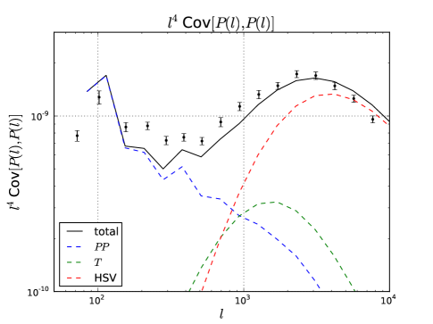
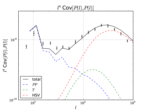
Figure 1: Comparison of our analytical prediction for the lensing power spectrum covariance (Eqs. 34 and 20) with the ray-tracing simulation results obtained from 1000 realizations. Here we considered a single source redshift $z_{s}=1$. For the analytical predictions, the Gaussian term (PP), the trispectrum term (T) and the halo sample variance (HSV) are included. The error bars for the simulation results are obtained from the variance of the 1000 realizations, which correspond to $1\sigma$ scatters of power spectrum estimation for 25 square degrees, the area of each ray-tracing simulation. Left panel: We included only the 1-halo term for the HSV calculation. Right: We further included the 2-halo term contribution for the HSV effect. The analytical predictions are in fairly good agreement with the simulation results, over a wide range of multipoles, if the HSV effect is included in the analytical prediction. Comparing the left and right panels shows that including the 2-halo term of the HSV effect improves the agreement at the transition regime between the 1- and 2-halo terms, in the range of $l\simeq$a few hundreds to $10^{3}$.

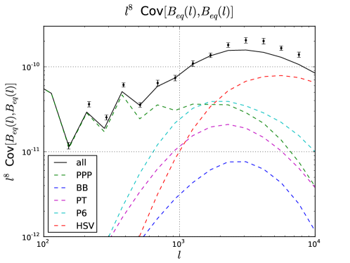
Figure 2: Comparison of the halo model prediction with the simulation results for the lensing bispectrum covariance for equilateral triangle configurations, as a function of the side length. For the analytical model, we included the standard Gaussian and non-Gaussian contributions arising from a combination of the correlation functions up to the 6-point correlation function (PPP, BB, PT, P6, from Eq 54) and also included the HSV contribution (Eq. 34). For the HSV contribution, we included all 1-, 2- and 3-halo terms, but only the 1=halo term gives an important contribution.

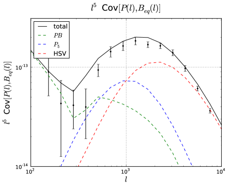
Figure 3: Cross-covariance between the lensing power spectrum, $P_{\kappa}(l)$, and the bispectrum of equilateral triangle configuration, $B_{\rm eq}(l,l,l)$, against multipoles. Similarly to the previous plot, for the halo model prediction, we included the standard contributions (PB, P5, from Eq. 55) and the HSV contribution (Eq. 34).

Fig. 1 shows the diagonal elements of the power spectrum covariance as a function of multipole. The halo model predictions are in fairly good agreement with the simulation results. This agreement can be realized only if including the HSV contribution. The right panel shows the results for the halo model when including the HSV contributions for the 2-halo term, which can be compared with the previous study such as Ref. Sato et al. (2009). The figure shows that including the HSV 2-halo term improves the agreement over a range of the transition regime between the 1- and 2-halo terms. Note that these results are for survey area of 25 sq. degrees, the area of the ray-tracing simulations we use (see Section IV.2), but the HSV effects are significant for any survey area of upcoming surveys (see Refs. Kayo et al. (2012); Takada and Hu (2013)).

In Figs. 2 and 3, we show the results for the bispectrum covariance and the cross-covariance between power spectrum and bispectrum. We followed the method in Ref. Kayo et al. (2012), and for both the figures we considered the bispectra of equilateral triangle configurations against the side length. The halo model is again in good agreement with the simulations, to a level of 10–20% accuracy in their amplitudes.

IV.3.3 Cross-covariances between angular number counts of halos and the lensing $n$-point correlation functions

Applying the formulation for 3D fields in Section III.3 to 2D fields, we can estimate the cross-covariance between the angular number counts of clusters and the lensing power spectrum:

$$\text{Cov}[\hat{N}_{M>M_{\rm th}},\hat{P}^{\kappa}(l)] = \int_{0}^{\chi_{S}}d\chi\,\,\,\frac{q^{2}(\chi)}{\chi^{2}}\left[\sum_{i>i_{min}}\bar{n}_{i}p_{i}^{1h}(k)+2\sum_{i>i_{min},j}\bar{n}_{i}\bar{n}_{j}p_{ij}^{2h}(k)\right]$$ (35)

$$+\Omega_{S}\int_{0}^{\chi_{S}}d\chi\,\,\,q^{2}(\chi)\left(\sum_{i>i_{min}}\bar{n}_{i}b_{i}\right)\frac{\partial\bar{P}(k)}{\partial\delta_{b}}d\sigma^{2}(\chi;\Omega_{S}),$$

where $k=l/\chi$ in the arguments on the r.h.s.

The cross-covariance for the lensing bispectrum is

$$\text{Cov}[\hat{N}_{M>M_{\rm th}},\hat{B}(\vec{l})] = \int_{0}^{\chi_{S}}d\chi\,\,\,\frac{q^{3}(\chi)}{\chi^{4}}\left[\sum_{i>i_{min}}\bar{n}_{i}b_{i}^{1h}(\vec{k})+2\sum_{i>i_{min},j}\bar{n}_{i}\bar{n}_{j}b_{ij}^{2h}(\vec{k})+3\sum_{i>i_{min},j,l}\bar{n}_{i}\bar{n}_{j}\bar{n}_{l}b_{ijl}^{3h}(\vec{k})\right]$$ (36)

$$+\Omega_{S}\int_{0}^{\chi_{S}}d\chi\,\,\,\frac{q^{3}(\chi)}{\chi^{2}}\left(\sum_{i>i_{min}}\bar{n}_{i}b_{i}\right)\frac{\partial\bar{B}(\vec{k})}{\partial\delta_{b}}d\sigma^{2}(\chi;\Omega_{S}),$$

where we have again used the collapsed notation such as $\vec{l}=(l_{1},l_{2},l_{3})$ and $\vec{k}=(l_{1}/\chi,l_{2}/\chi,l_{3}/\chi)$.

To be more general, the cross-covariance for the lensing $N$-point correlation function is given as

$$\text{Cov}[\hat{N}_{M>M_{\rm th}},\hat{P}_{N}] = \int_{0}^{\chi_{S}}d\chi\,\,\,\frac{q^{N}(\chi)}{\chi^{2(N-1)}}\left[\sum_{i>i_{min}}\bar{n}_{i}p_{i}^{1h}+2\sum_{i>i_{min},j}\bar{n}_{i}\bar{n}_{j}p_{ij}^{2h}+...\right.$$

$$\left.+N\sum_{i_{1}>i_{min},i_{2},...,i_{N}}\bar{n}_{i_{1}}\bar{n}_{i_{2}}...\bar{n}_{i_{N}}p_{i_{1},i_{2},...,i_{N}}^{Nh}\right]+\Omega_{S}\int_{0}^{\chi_{S}}d\chi\,\,\,\frac{q^{N}(\chi)}{\chi^{2(N-2)}}\left(\sum_{i>i_{min}}\bar{n}_{i}b_{i}\right)\frac{\partial\bar{P}_{N}}{\partial\delta_{b}}d\sigma^{2}(\chi;\Omega_{S}).$$

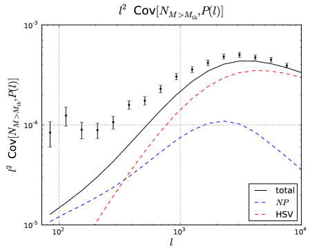
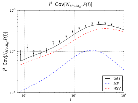
Figure 4: Cross-covariance between the angular number counts of halos and the lensing power spectrum $P_{\kappa}(l)$ as a function of multipoles. For the number counts, we included all the halos that are in the light cone up to $z_{s}=1$ over area 25 sq. degrees (area of the ray-tracing simulation) and have masses greater than $M=10^{14}M_{\odot}/h$. The error bars for the simulation results are the variance estimated from the 1000 realizations. For the halo model prediction, we used Eq. (35) to compute the contributions arising from the product of the number counts and the power spectrum (NP) and the HSV effect. The difference between the left and right panels is whether the halo model prediction includes the 2-halo term of the HSV effect (right) or not (left). The halo model prediction, with the 2-halo HSV effect, well reproduces the simulation result over the range of multipoles.

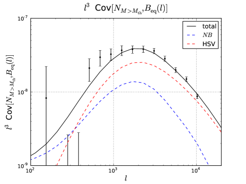
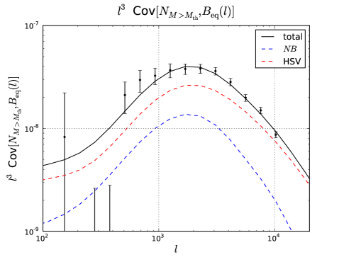
Figure 5: Similarly to the previous plot, the cross-covariance between the angular halo number counts and the bispectrum of equilateral triangle configurations, $B_{\kappa,{\rm eq}}(l,l,l)$. The halo model computation is based on Eq. (36). The difference between the left and right panels is whether we included the 2- and 3-halo terms for the HSV contribution in the halo model prediction (right panel) or not (left).

In Figs. 4 and 5, we compare the halo model predictions for the cross-covariance of the angular number counts of halos with the lensing power spectrum or bispectrum. For the halo number counts, we included all the halos that are in the light cone up to $z_{s}=1$ and over area of 25 square degrees (area of the ray-tracing simulation). Both figures show that the halo model predictions are in fairly nice agreement with the simulation results, if including the HSV contribution. It is also shown that including the different halo terms of the HSV effect better agrees with the simulation results over a range of the transition regime of multipoles between the 1-halo term and the different halo terms.

V Joint likelihood for power spectrum, bispectrum and cluster counts, and Fisher forecast

We have so far derived the co- or cross-variances between the halo number counts, the power spectrum and the bispectrum. In this section, we discuss their joint likelihood function. Exactly speaking, a derivation of the likelihood function requires a knowledge on all the higher-order cumulants of the observables beyond the second-order moments such as the skewness and kurtosis. Here, we instead assume that the joint likelihood function obeys a multivariate Gaussian function that is given by the mean values and the second-order variances (co- or cross-covariances) of the observables, which we have already derived up to the previous section. The multivariate Gaussian likelihood is somewhat expected for the lensing fields at high multipoles due to the central limit theorem, because the lensing field is from a projection of independent large-scale structure at different redshifts along the line-of-sight and also because the power spectrum and bispectrum of high multipoles are from the averages over a large number of Fourier modes.

Thus we assume that the joint likelihood function for observables $D$ obeys the following multivariate Gaussian:

$$\mathcal{L}\left(\mbox{\boldmath$D$}\right)\propto\text{exp}\left[-\frac{1}{2}\left(\mbox{\boldmath$D$}-\bar{\mbox{\boldmath$D$}}\right)^{t}\mbox{\boldmath$\Sigma$}^{-1}\left(\mbox{\boldmath$D$}-\bar{\mbox{\boldmath$D$}}\right)\right],$$ (38)

where $D$ denotes the observable vector, e.g. defined a $\mbox{\boldmath$D$}\equiv\left(\{\hat{P}(l)\},\{\hat{B}(l)\},\hat{N}_{M>M_{\rm th}}\right)$, $\bar{\mbox{\boldmath$D$}}$ denotes its mean vector, $\Sigma$ its co- or cross-variance matrix, and $\mbox{\boldmath$\Sigma$}^{-1}$ is the inverse matrix. The vector and matrix notations are intended to mean the summation over the cluster mass bin (a single bin though here), the multipole bins or the triangle configurations.

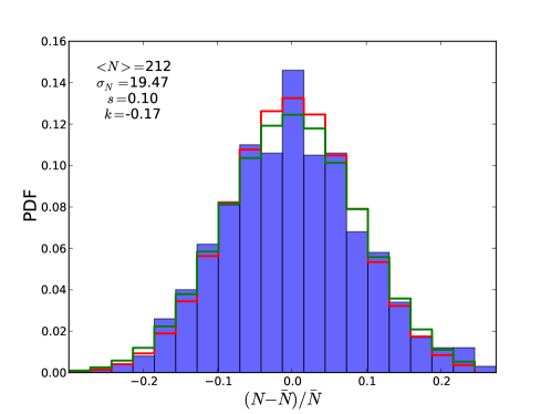
Figure 6: The likelihood distribution of the angular number counts of halos with $M\geq 10^{14}M_{\odot}/h$, in the light-cone up to $z_{s}=1$ and with area $25$ sq. degrees. The histogram shows the distribution measured from the 1000 ray-tracing simulations. The red-color, solid curve shows the halo model prediction computed assuming the Gaussian likelihood function (Eq. 38), where we used the halo model to compute the mean and the variance. For comparison, the green-color, solid curve shows the Gaussian distribution that has the same mean value and variance as those of the simulations. The mean, variance, skewness and excess kurtosis values measured from the simulations are also given.

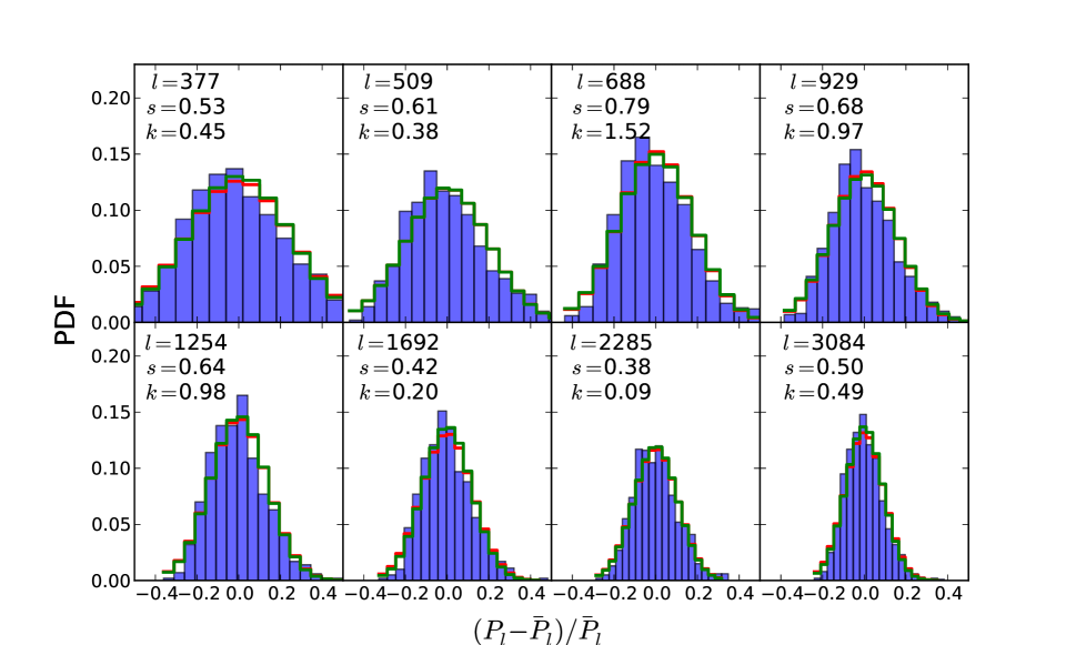
Figure 7: Similarly to the previous figure, but for the lensing power spectrum $P_{\kappa}(l)$. The different panels show the distributions for different multipole bins as indicated. Again the halo model prediction (red, solid curve) well reproduces the width of the simulation distribution, if the HSV contribution is included. The skewness and kurtosis measured from simulations are small compared to the width of the distribution.

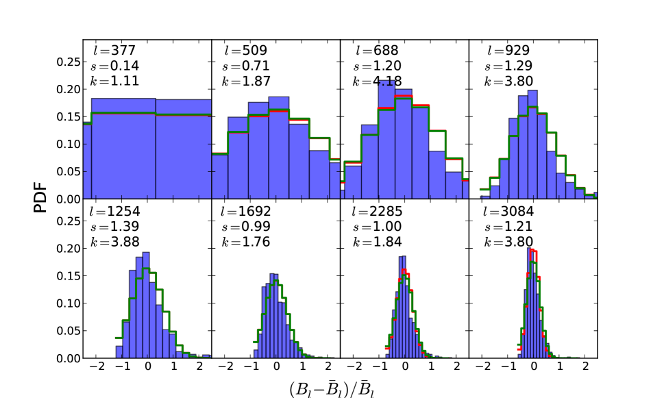
Figure 8: Similarly to the previous plot, but for the lensing bispectrum of equilateral triangle configurations. The different panels are for different-size triangle configurations. Compared to Figs. 6 and 7, the simulation distribution shows a larger asymmetry and therefore larger skewness and kurtosis values. The halo model nevertheless well reproduces the width of the distribution.

In Figs. 6, 7 and 8, we show the distributions of the angular number counts of halos, the lensing power spectrum, and the bispectrum of equilateral triangles, which we measured from the 1000 ray-tracing simulations. Again note that the distributions are for the area of 25 sq. degrees. These observables show a fairly symmetric distribution, although the bispectrum shows a larger skewness than the other two quantities. The red-color solid curve in each figure shows the halo model prediction (Eq. 38). The halo model appears to well reproduce the width of the distribution seen in the simulations. The agreement is realized only if we include the HSV contributions as shown in Figs. 1 and 2. These figures also show that the skewness of the distribution is well within the width of the distribution.

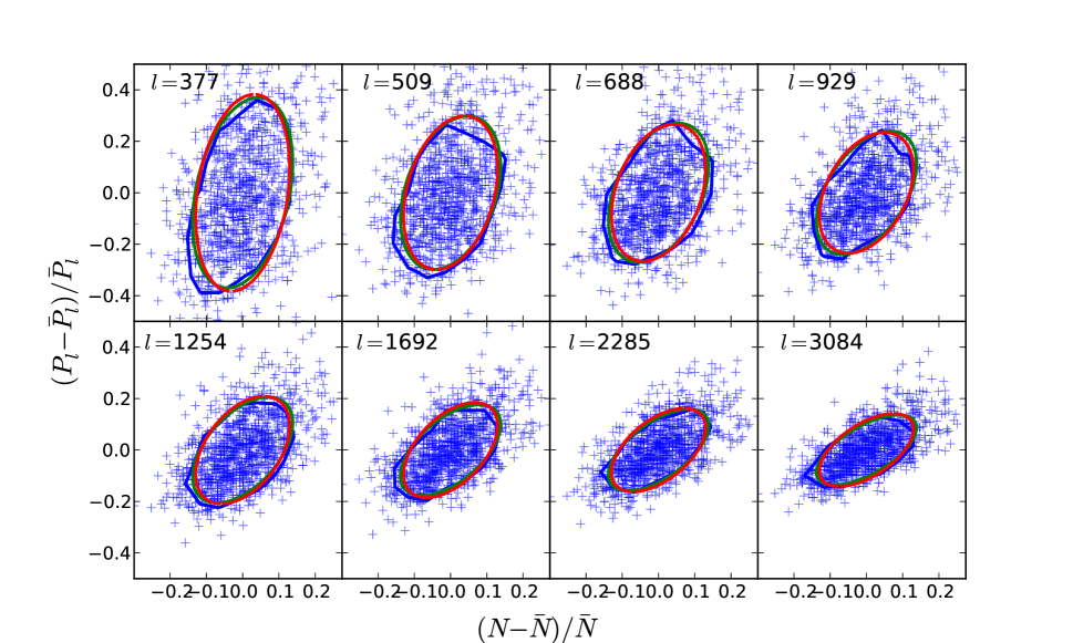
Figure 9: A joint distribution of the angular number counts of halos with $M\geq 10^{14}M_{\odot}$ and the lensing power spectrum $P_{\kappa}(l)$. The different panels show the results for different multipole bins as denoted. Each cross symbol denotes one realization out of the 1000 realizations. The blue-color contour in each panel shows the 68% percentile of the distribution, which is estimated by binning the 1000 simulations into a 2d-histogram. The red-color contour shows the halo model prediction for the joint distribution, computed based on Eq. (38). For comparison, the green contour shows the multivariate Gaussian distribution that has the same mean and variances as those of the simulation distribution.

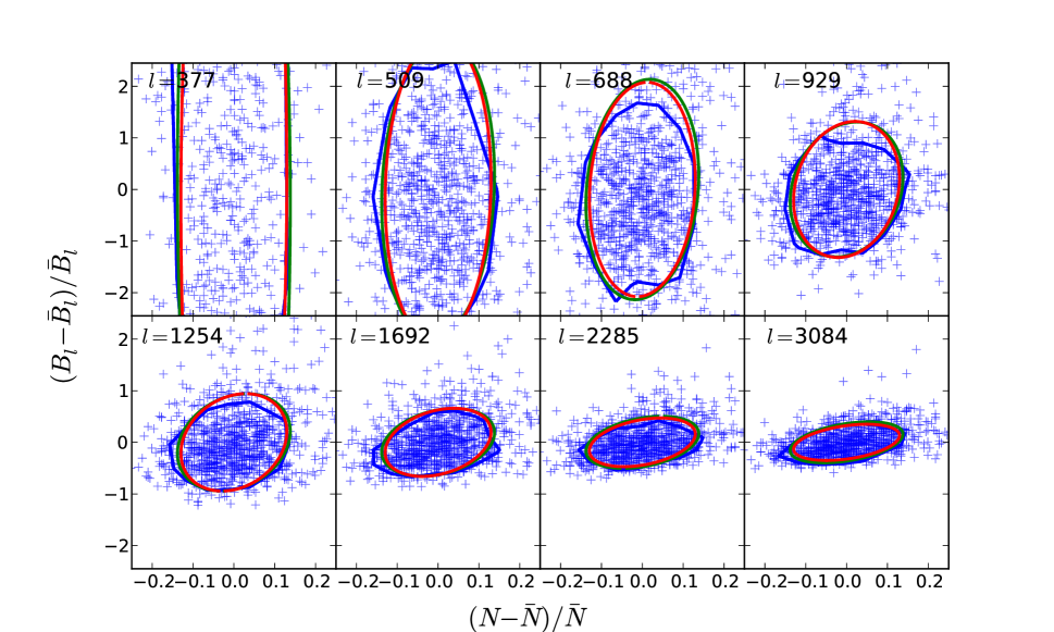
Figure 10: Similarly to the previous figure, but the joint distribution for the halo number counts and the lensing bispectrum of equilateral triangle configurations, $B_{\kappa,{\rm eq}}(l,l,l)$. The halo model well reproduces the distribution seen in the simulations.

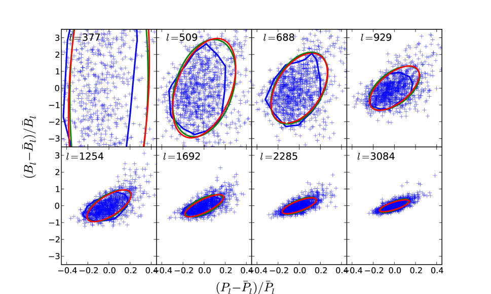
Figure 11: Similarly to the previous figure, but the joint distribution for the lensing power spectrum and bispectrum.

Figs. 9, 10 and 11 show the joint distributions for a combination of the angular number counts of halos, the lensing power spectrum, or the lensing bispectrum of equilateral triangle configurations. The halo model fairly well reproduces the joint distributions over a range of multipoles (the width and the direction of the cross-correlation). However, we note that the agreement for the bispectrum is not relatively as good as for the power spectrum, reflecting the limitation of the multivariate Gaussian assumption for the bispectrum distribution.

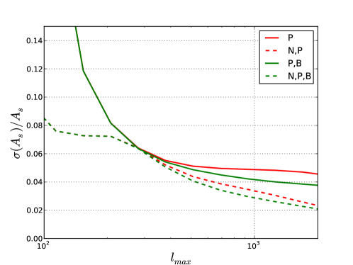
Figure 12: Forecast error on the amplitude of scalar perturbations $A_{S}$ as a function of the maximum observed multipole $l_{\text{max}}$, when marginalizing over $\Omega_{m}$, and keeping all other parameters fixed. We here assumed a hypothetical survey that is characterized by area $15000$ sq. deg. and the redshift distribution following Oguri and Takada (2011) with $\left\langle z_{s}\right\rangle=3z_{0}=1$. We included the galaxy shape noise contamination, assuming $\sigma_{\epsilon}=0.22$ and $n_{\text{gal}}=20\text{arcmin}^{-2}$ for the number density and the rms intrinsic elllipticities. The solid red curve shows the error when including the power spectrum information alone. The solid-green and dashed curves show the results when further including the bispectrum measurements of equilateral triangle configuration and the cluster number counts.

Having found that the halo model fairly well describes the joint likelihood functions between the cluster number counts and the lensing correlation functions, we now discuss how a future survey can improve cosmological constraints based on the joint measurements of the different observables obtained from the same survey data. As one demonstration, we consider only two cosmological parameters, the matter density parameter $\Omega_{\rm m}$ and the amplitude parameter of the primordial curvature perturbation $A_{s}$, both of which are sensitive to the amplitudes of the number counts and the lensing correlation functions and therefore are most affected by the HSV effect. However, note that we fix all other parameters to their fiducial values. Assuming the multivariate Gaussian likelihood, we use the Fisher information matrix formalism to perform a parameter forecast:

$$F_{ij}=\frac{\partial\mbox{\boldmath$D$}^{t}}{\partial p_{i}}\mbox{\boldmath$\Sigma$}^{-1}\frac{\partial\mbox{\boldmath$D$}}{\partial p_{j}},$$ (39)

where $p_{i}$ denotes the $i$-th cosmological parameter ($\Omega_{\rm m}$ or $A_{s}$). To make parameter forecast for a hypothetical future survey, we include the shape noise contamination to the lensing power spectrum and bispectrum covariances for which we model assuming $\bar{n}_{g}=20~{}$arcmin^-2 and $\sigma_{\epsilon}=0.22$ for the mean number density of source galaxies and the rms intrinsic ellipticities, respectively. We assume $\Omega_{S}=15,000$ sq. degrees for survey area, and model the redshift distribution of source galaxies by an analytical model that is given by $\left\langle z_{s}\right\rangle=3z_{0}=1$ in Eq. (17) in Oguri & Takada Oguri and Takada (2011). These survey parameters resemble those expected for a Euclid-type survey.

Fig. 12 shows the expected precision of $A_{s}$ including marginalization over $\Omega_{\rm m}$, as a function of maximum multipole up to which we include the power spectrum information (and also the lensing bispectrum). Note that, for the bispectrum, we included all the equilateral triangle configurations available over a range of multipoles up to a given maximum multipole, but did not include other triangle information. The figure shows that combining the cluster number counts with the power spectrum and bispectrum measurements for $l_{\rm max}=1000$, which is the target maximum multipole for the Euclid survey, tightens the error by a factor of $30$–$40\%$. This improvement is equivalent to a factor 2 wider survey area.

VI Conclusion

In this paper, we presented a simple and general formalism to compute the halo sample variances for the cluster counts, and any $n$-point function for the matter density or any projected density field, such as cosmic shear or the thermal Sunyaev-Zel’dovich effect. These results rely only on the assumptions built into the halo model, provide a good fit to the simulation from Ref. Sato et al. (2009), and allow for an intuitive understanding of all the terms.

We presented a simple ansatz for the joint likelihood of cluster counts, power spectrum and bispectrum of the lensing convergence, and showed its relatively good agreement with simulation. We used this joint likelihood to estimate that constraints on cosmological parameters such as $\Omega_{m}$ and $A_{s}$ can be improved by $30\%$ ($40\%$) if one combines the cluster counts with the power spectrum measurement (further combined with the lensing bispectrum). This is equivalent to doubling the survey volume.

Taking into account the specific geometry of the survey (and not only its volume), as well as the selection functions for the cluster counts and the uncertainty on the mass determination, constitute interesting extensions of this study which we leave for future work.

Acknowledgments.– We thank Issha Kayo for providing us with his analyzed data from the simulations in Sato et al. (2009), and for his help and kindness throughout this project. ES would like to thank Elisabeth Krause for helpful discussion, Simone Ferraro for his many useful comments throughout this project as well as reading an early version of this paper, and the Kavli IPMU for their hospitality. DNS and ES acknowledge support from NSF Grant AST-1311756, NASA Grant 11-ATP-090, NASA ROSES grant 12-EUCLID12-0004 and the Euclid Consortium. MT was supported by World Premier International Research Center Initiative (WPI Initiative), MEXT, Japan, by the FIRST program “Subaru Measurements of Images and Redshifts (SuMIRe)”, CSTP, Japan, and by Grant-in-Aid for Scientific Research from the JSPS Promotion of Science (No. 23340061 and 26610058).

Appendix A Matter $N$-point functions: expectation values and covariances

A.1 Expectation values: halo decomposition

In this subsection we derive the expectation value of our power spectrum estimator without using the general results from Section II.3, in order to see in more details why the expectation value is not affected by the finite size effect. The same reasoning applies to any $n$-point function as we shall explain.

Our estimator for the power spectrum is given by Eq (18), where the matter overdensity is described in the halo model by Eq (2). The expectation value for the power spectrum estimator is obtained directly from:

$$\left\langle\hat{\delta}(\vec{q}_{1})\hat{\delta}(\vec{q}_{2})\right\rangle =\left\langle\sum_{i,j}\left(\frac{m_{i}m_{j}}{\bar{\rho}^{2}}\right)u_{i}(\vec{q}_{1})u_{j}(\vec{q}_{2})\,\,\hat{n}_{i}(\vec{q}_{1},\delta_{b})\hat{n}_{j}(\vec{q}_{2},\delta_{b})\right\rangle$$ (40)

$$=\sum_{i,j}\left(\frac{m_{i}m_{j}}{\bar{\rho}^{2}}\right)u_{i}(\vec{q}_{1})u_{j}(\vec{q}_{2})\,\,\left\langle\hat{n}_{i}(\vec{q}_{1},\delta_{b})\hat{n}_{j}(\vec{q}_{2},\delta_{b})\right\rangle.$$

Thus we only need to compute the quantity $\left\langle\hat{n}_{i}(\vec{q}_{1},\delta_{b})\hat{n}_{j}(\vec{q}_{2},\delta_{b})\right\rangle$. We decompose the averaging procedure into marginalizing over the Poisson sampling, then the underlying density $\rho_{\text{lin}}$, and eventually the local average overdensity $\delta_{b}$. The First average is obtained from Eq (4), and gives the usual Poisson shot noise:

$$\left\langle\hat{n}_{i}(\vec{x}_{1})\hat{n}_{j}(\vec{x}_{2})\right\rangle_{\text{Pois.}} =n_{i}(\vec{x}_{1})n_{j}(\vec{x}_{2})+\delta^{K}_{i,j}\delta_{D}(\vec{x}_{1}-\vec{x}_{2})n_{i}(\vec{x}),$$ (41)

where again, we defined $n_{i}(\vec{x})\equiv\left\langle\hat{n}_{i}(\vec{x})\right\rangle_{\text{Pois.}}$. After Fourier transform, this becomes:

$$\left\langle\hat{n}_{i}(\vec{q}_{1})\hat{n}_{j}(\vec{q}_{2})\right\rangle_{\text{Pois.}} =n_{i}(\vec{q}_{1})n_{j}(\vec{q}_{2})+\delta^{K}_{i,j}n_{i}(\vec{q}_{1}+\vec{q}_{2}).$$ (42)

Averaging over the underlying density field at fixed $\delta_{b}$ gives:

$$\left\langle\hat{n}_{i}(\vec{q}_{1})\hat{n}_{j}(\vec{q}_{2})\right\rangle_{\text{Pois.},{\rho_{\text{lin}}}|\delta_{b}} =\left\langle n_{i}(\vec{q}_{1})n_{j}(\vec{q}_{2})\right\rangle_{{\rho_{\text{lin}}}|\delta_{b}}+\delta^{K}_{i,j}\bar{n}_{i}(\delta_{b})\left(2\pi\right)^{3}\delta_{D}(\vec{q}_{1}+\vec{q}_{2})$$ (43)

$$=\bar{n}_{i}(\delta_{b})\bar{n}_{j}(\delta_{b})\left\langle\delta^{h}_{i}(\vec{q}_{1})\delta^{h}_{j}(\vec{q}_{2})\right\rangle_{{\rho_{\text{lin}}}|\delta_{b}}+\delta^{K}_{i,j}\bar{n}_{i}(\delta_{b})\left(2\pi\right)^{3}\delta_{D}(\vec{q}_{1}+\vec{q}_{2})$$

$$=\left[\bar{n}_{i}(\delta_{b})\bar{n}_{j}(\delta_{b})b_{i}b_{j}P_{\text{lin}}(q_{1})+\delta^{K}_{i,j}\bar{n}_{i}(\delta_{b})\right]\left(2\pi\right)^{3}\delta_{D}(\vec{q}_{1}+\vec{q}_{2}).$$

Here, we introduced the usual halo number overdensity $\delta_{i}^{h}$ for halos of mass $m_{i}$, and used the linear bias to write $\left\langle\delta_{i}^{h}\delta_{j}^{h}\right\rangle=\left(2\pi\right)^{3}\delta_{D}b_{i}b_{j}P_{\text{lin}}$. Switching to discrete Fourier transform, this becomes:

$$\left\langle\hat{n}_{i}(\vec{q}_{1})\hat{n}_{j}(\vec{q}_{2})\right\rangle_{\text{Pois.},{\rho_{\text{lin}}}|\delta_{b}}=\left[\bar{n}_{i}(\delta_{b})\bar{n}_{j}(\delta_{b})b_{i}b_{j}P_{\text{lin}}(q_{1})+\delta^{K}_{i,j}\bar{n}_{i}(\delta_{b})\right]V_{S}\delta^{K}_{\vec{q}_{1}+\vec{q}_{2}}.$$ (44)

Hence the expectation value of the power spectrum at fixed $\delta_{b}$:

$$\left\langle\hat{P}(k)\right\rangle_{|\delta_{b}} =\sum_{i,j}\left(\frac{m_{i}m_{j}}{\bar{\rho}^{2}}\right)u_{i}(k)u_{j}(k)\,\,\bar{n}_{i}(\delta_{b})\bar{n}_{j}(\delta_{b})b_{i}b_{j}P_{\text{lin}}(k)\,\,+\,\,\sum_{i}\left(\frac{m_{i}}{\bar{\rho}}\right)^{2}|u_{i}(k)|^{2}\,\,\bar{n}_{i}(\delta_{b}).$$ (45)

This is nothing but the halo decomposition $P=P^{1h}+P^{2h}$, except for the extra $\delta_{b}$-dependence. To marginalize over $\delta_{b}$, we simply use Eq (7):

$$\left\langle\hat{P}(k)\right\rangle =\sum_{i,j}\left(\frac{m_{i}m_{j}}{\bar{\rho}^{2}}\right)u_{i}(k)u_{j}(k)\,\,\bar{n}_{i}\bar{n}_{j}\left[1+\sigma_{m}^{2}b_{i}b_{j}\right]b_{i}b_{j}P_{\text{lin}}(k)\,\,+\,\,\sum_{i}\left(\frac{m_{i}}{\bar{\rho}}\right)^{2}|u_{i}(k)|^{2}\,\,\bar{n}_{i}.$$ (46)

This averaging procedure is equivalent to the one described by eq (9) in Section II.3. Provided that $\sigma_{m}^{2}b_{i}b_{j}\ll 1$, we see that the finite size of the box does not lead to any significant bias in our power spectrum estimator.

The same reasoning applies for any $n$-point function: one can disregard the effect of $\delta_{b}$ when computing expectation values, and using the Poisson property Eq (4) leads to the standard halo decomposition $P_{N}=P_{N}^{1h}+...+P_{N}^{Nh}$.

A.2 Covariances

In this subsection, we derive and discuss the general result Eq (14). We start with observables $\hat{f}$ and $\hat{g}$ that are determined by the halo counts $\left\{\hat{n}_{i}(\vec{x})\right\}$, and we call $\bar{f}(\delta_{b})=\left\langle\hat{f}\right\rangle_{\delta_{b}}$ (and similarly for $\hat{g}$). We Taylor expand $\bar{f}$ (and $\bar{g}$) around $\delta_{b}=0$:

$$\bar{f}(\delta_{b})=\bar{f}(0)+\left.\frac{\partial\bar{f}}{\partial\delta_{b}}\right|_{\delta_{b}=0}\delta_{b}+\frac{1}{2}\left.\frac{\partial^{2}\bar{f}}{\partial\delta_{b}^{2}}\right|_{\delta_{b}=0}\delta_{b}^{2}+\mathcal{O}(\delta_{b}^{3}),$$ (47)

marginalizing over $\delta_{b}$ then yields:

$$\left\langle\bar{f}(\delta_{b})\right\rangle=\bar{f}(0)+\frac{1}{2}\left.\frac{\partial^{2}\bar{f}}{\partial\delta_{b}^{2}}\right|_{\delta_{b}=0}\sigma_{m}^{2}+\mathcal{O}(\sigma_{m}^{4}),$$ (48)

and:

$$\left\langle\bar{f}(\delta_{b})\bar{g}(\delta_{b})\right\rangle=\left\langle\bar{f}(\delta_{b})\right\rangle\left\langle\bar{g}(\delta_{b})\right\rangle+\left.\frac{\partial\bar{f}}{\partial\delta_{b}}\right|_{\delta_{b}=0}\left.\frac{\partial\bar{g}}{\partial\delta_{b}}\right|_{\delta_{b}=0}\sigma_{m}^{2}+\mathcal{O}(\sigma_{m}^{4}).$$ (49)

Deriving relation (13) is now straightforward:

$$\text{Cov}\left[\hat{f},\hat{g}\right] \equiv\left\langle\left\langle\hat{f}\hat{g}\right\rangle_{|\delta_{b}}\right\rangle_{\delta_{b}}-\left\langle\left\langle\hat{f}\right\rangle_{|\delta_{b}}\right\rangle_{\delta_{b}}\left\langle\left\langle\hat{g}\right\rangle_{|\delta_{b}}\right\rangle_{\delta_{b}}$$ (50)

$$=\left\langle\left\langle\hat{f}\hat{g}\right\rangle_{|\delta_{b}}\right\rangle_{\delta_{b}}-\left\langle\bar{f}(\delta_{b})\right\rangle_{\delta_{b}}\left\langle\bar{g}(\delta_{b})\right\rangle_{\delta_{b}}$$

$$=\left\langle\left\langle\hat{f}\hat{g}\right\rangle_{|\delta_{b}}\right\rangle_{\delta_{b}}-\left\langle\bar{f}(\delta_{b})\bar{g}(\delta_{b})\right\rangle_{\delta_{b}}+\left.\frac{\partial\bar{f}}{\partial\delta_{b}}\right|_{\delta_{b}=0}\left.\frac{\partial\bar{g}}{\partial\delta_{b}}\right|_{\delta_{b}=0}\sigma_{m}^{2}+\mathcal{O}(\sigma_{m}^{4})$$

$$=\left\langle\left\langle\hat{f}\hat{g}\right\rangle_{|\delta_{b}}-\bar{f}(\delta_{b})\bar{g}(\delta_{b})\right\rangle_{\delta_{b}}+\left.\frac{\partial\bar{f}}{\partial\delta_{b}}\right|_{\delta_{b}=0}\left.\frac{\partial\bar{g}}{\partial\delta_{b}}\right|_{\delta_{b}=0}\sigma_{m}^{2}+\mathcal{O}(\sigma_{m}^{4})$$

$$=\left\langle\text{Cov}\left[\hat{f},\hat{g}\right]_{|\delta_{b}}\right\rangle_{\delta_{b}}+\left.\frac{\partial\bar{f}}{\partial\delta_{b}}\right|_{\delta_{b}=0}\left.\frac{\partial\bar{g}}{\partial\delta_{b}}\right|_{\delta_{b}=0}\sigma_{m}^{2}+\mathcal{O}(\sigma_{m}^{4}).$$

And as we’ve seen, marginalizing over $\delta_{b}$ reduces to the substitution (9), which leads to negligible terms (in the same exact way as in the example of the power spectrum expectation value above). Hence we get Eq (14):

$$\text{Cov}\left[\hat{f},\hat{g}\right]\simeq\text{Cov}\left[\hat{f},\hat{g}\right]_{\text{Pois.},\rho_{\text{lin}}|\delta_{b}=0}+\sigma_{m}^{2}\left.\frac{\partial\bar{f}}{\partial\delta_{b}}\right|_{\delta_{b}=0}\left.\frac{\partial\bar{g}}{\partial\delta_{b}}\right|_{\delta_{b}=0}.\\$$ (51)

The second term is the halo sample variance, and is readily computed from the halo decomposition of the $N$-point functions and linear biasing. The first term is the standard covariance. It is computed by using the expression of our estimator as a product of $\hat{\delta}$, and the decomposition of correlation functions into connected correlation functions Bernardeau et al. (2002):

$$\left\langle\hat{\delta}(\vec{x}_{1})...\hat{\delta}(\vec{x}_{n})\right\rangle =\left\langle\hat{\delta}(\vec{x}_{1}),...,\hat{\delta}(\vec{x}_{n})\right\rangle_{c}+\sum_{S}\prod_{s_{i}\in S}\left\langle\hat{\delta}_{s_{i}(1)},...,\hat{\delta}_{s_{i}(\#s_{i})}\right\rangle_{c},$$ (52)

where the sum is over all the proper partitions of $\{1,...,n\}$. This yields the following standard covariance for the power spectrum:

$$\text{Cov}\left[\hat{P}(k),\hat{P}(k^{\prime})\right]_{|\delta_{b}=0} =\frac{2\delta^{K}_{k,k^{\prime}}}{N(k)}\bar{P}^{2}(k)+\frac{1}{V_{S}}\bar{T}(\vec{q},-\vec{q},\vec{q}^{\,\prime},-\vec{q}^{\,\prime})^{\|\vec{q}\|\simeq k,\|\vec{q}^{\prime}\|\simeq k^{\prime}}.$$ (53)

This procedure also yields the results of Kayo et al. (2012) for the bispectrum covariance:

$$\text{Cov}\left[\hat{B}_{(k_{1},k_{2},k_{3})},\hat{B}_{(k_{1}^{\prime},k_{2}^{\prime},k_{3}^{\prime})}\right]_{|\delta_{b}=0}=V_{S}\frac{\delta^{K}_{k_{1},k_{1}^{\prime}}\delta^{K}_{k_{2},k_{2}^{\prime}}\delta^{K}_{k_{3},k_{3}^{\prime}}}{N_{\Delta}(k_{1},k_{2},k_{3})}\,\bar{P}_{(k_{1})}\bar{P}_{(k_{2})}\bar{P}_{(k_{3})}+\text{5 permutations of the }k_{i^{\prime}}$$ (54)

$$\hskip 42.67912pt+\frac{\delta^{K}_{k_{1}^{\prime},k_{3}}}{N_{\Delta}(k_{1},k_{2},k_{3})N_{\Delta}(k_{1}^{\prime},k_{2}^{\prime},k_{3}^{\prime})}\sum_{1,2,3\atop 2^{\prime},3^{\prime}}\delta^{K}_{1+2+3}\delta^{K}_{3+2^{\prime}+3^{\prime}}\,\bar{B}_{(1,2,3)}\,\bar{B}_{(3,2^{\prime},3^{\prime})}+\text{8 permutations}$$

$$\hskip 42.67912pt+\frac{\delta^{K}_{k_{1},k_{1}^{\prime}}}{N_{\Delta}(k_{1},k_{2},k_{3})N_{\Delta}(k_{1}^{\prime},k_{2}^{\prime},k_{3}^{\prime})}\sum_{1,2,3\atop 2^{\prime},3^{\prime}}\delta^{K}_{1+2+3}\delta^{K}_{-1+2^{\prime}+3^{\prime}}\,\bar{P}_{(1)}\,\bar{T}_{(2,2^{\prime},3,3^{\prime})}+\text{8 different choices }(i,j^{\prime})$$

$$\hskip 42.67912pt+\frac{1}{V_{S}}\frac{1}{N_{\Delta}(1,2,3)N_{\Delta}(1^{\prime},2^{\prime},3^{\prime})}\sum_{1,2,3\atop 1^{\prime},2^{\prime},3^{\prime}}\delta^{K}_{1+2+3}\delta^{K}_{1^{\prime}+2^{\prime}+3^{\prime}}\bar{P}_{6}(1,2,3,1^{\prime},2^{\prime},3^{\prime}).$$

As well as their result for the cross-covariance between power spectrum and bispectrum:

$$\text{Cov}\left[\hat{P}_{(k)},\hat{B}_{(k_{1},k_{2},k_{3})}\right]_{|\delta_{b}=0} =\frac{2\delta^{K}_{k,k_{1}}}{N(k_{1})}\bar{P}(k_{1})\bar{B}(k_{1},k_{2},k_{3})+\text{2 perm.}$$ (55)

$$+\frac{1}{V_{S}}\int\frac{d\psi}{2\pi}\bar{P}_{5}(k,-k,k_{1},k_{2},k_{3}),$$

where $\psi$ is the angle between $\vec{k}$ and $\vec{k}_{1}$.

References

- Note (1) http://cosmology.lbl.gov/BOSS/.
- Note (2) http://www.astro-wise.org/projects/KIDS/.
- Note (3) http://www.sdss3.org/future/eboss.php.
- Note (4) http://www.darkenergysurvey.org.
- The Dark Energy Survey Collaboration (2005) The Dark Energy Survey Collaboration, ArXiv Astrophysics e-prints (2005), arXiv:astro-ph/0510346 .
- Note (5) http://www.naoj.org/Projects/HSC/index.html.
- Miyazaki et al. (2006) S. Miyazaki, Y. Komiyama, H. Nakaya, Y. Doi, H. Furusawa, P. Gillingham, Y. Kamata, K. Takeshi, and K. Nariai, in Society of Photo-Optical Instrumentation Engineers (SPIE) Conference Series, Society of Photo-Optical Instrumentation Engineers (SPIE) Conference Series, Vol. 6269 (2006).
- Note (6) http://sumire.ipmu.jp/en/2652.
- Takada et al. (2012) M. Takada, R. Ellis, M. Chiba, J. E. Greene, H. Aihara, N. Arimoto, K. Bundy, J. Cohen, O. Doré, G. Graves, J. E. Gunn, T. Heckman, C. Hirata, P. Ho, J.-P. Kneib, O. Le Fèvre, L. Lin, S. More, H. Murayama, T. Nagao, M. Ouchi, M. Seiffert, J. Silverman, L. Sodré, Jr, D. N. Spergel, M. A. Strauss, H. Sugai, Y. Suto, H. Takami, and R. Wyse, ArXiv e-prints (2012), arXiv:1206.0737 [astro-ph.CO] .
- Note (7) http://desi.lbl.gov.
- LSST Science Collaboration et al. (2009) LSST Science Collaboration, P. A. Abell, J. Allison, S. F. Anderson, J. R. Andrew, J. R. P. Angel, L. Armus, D. Arnett, S. J. Asztalos, T. S. Axelrod, and et al., ArXiv e-prints (2009), arXiv:0912.0201 [astro-ph.IM] .
- Laureijs et al. (2011) R. Laureijs, J. Amiaux, S. Arduini, J. . Auguères, J. Brinchmann, R. Cole, M. Cropper, C. Dabin, L. Duvet, A. Ealet, and et al., ArXiv e-prints (2011), arXiv:1110.3193 [astro-ph.CO] .
- Spergel et al. (2013) D. Spergel, N. Gehrels, J. Breckinridge, M. Donahue, A. Dressler, B. S. Gaudi, T. Greene, O. Guyon, C. Hirata, J. Kalirai, N. J. Kasdin, W. Moos, S. Perlmutter, M. Postman, B. Rauscher, J. Rhodes, Y. Wang, D. Weinberg, J. Centrella, W. Traub, C. Baltay, J. Colbert, D. Bennett, A. Kiessling, B. Macintosh, J. Merten, M. Mortonson, M. Penny, E. Rozo, D. Savransky, K. Stapelfeldt, Y. Zu, C. Baker, E. Cheng, D. Content, J. Dooley, M. Foote, R. Goullioud, K. Grady, C. Jackson, J. Kruk, M. Levine, M. Melton, C. Peddie, J. Ruffa, and S. Shaklan, ArXiv e-prints (2013), arXiv:1305.5425 [astro-ph.IM] .
- Jain and Seljak (1997) B. Jain and U. Seljak, Astrophys. J. 484, 560 (1997), astro-ph/9611077 .
- Jain et al. (2000) B. Jain, U. Seljak, and S. White, Astrophys. J. 530, 547 (2000), astro-ph/9901191 .
- Scoccimarro et al. (1999a) R. Scoccimarro, M. Zaldarriaga, and L. Hui, Astrophys. J. 527, 1 (1999a), arXiv:astro-ph/9901099 .
- Hu and White (2001) W. Hu and M. White, Astrophys. J. 554, 67 (2001), arXiv:astro-ph/0010352 .
- Cooray and Hu (2001) A. Cooray and W. Hu, Astrophys. J. 554, 56 (2001), arXiv:astro-ph/0012087 .
- Takada and Jain (2004) M. Takada and B. Jain, Mon. Not. Roy. Astron. Soc. 348, 897 (2004), arXiv:astro-ph/0310125 .
- Takada and Jain (2009) M. Takada and B. Jain, Mon. Not. Roy. Astron. Soc. 395, 2065 (2009), arXiv:0810.4170 .
- Kayo et al. (2012) I. Kayo, M. Takada, and B. Jain, ArXiv e-prints (2012), arXiv:1207.6322 [astro-ph.CO] .
- Kayo and Takada (2013) I. Kayo and M. Takada, ArXiv e-prints (2013), arXiv:1306.4684 [astro-ph.CO] .
- Hamilton et al. (2006) A. J. S. Hamilton, C. D. Rimes, and R. Scoccimarro, Mon. Not. Roy. Astron. Soc. 371, 1188 (2006), arXiv:astro-ph/0511416 .
- Hu and Kravtsov (2003) W. Hu and A. V. Kravtsov, Astrophys. J. 584, 702 (2003), arXiv:astro-ph/0203169 .
- Sefusatti et al. (2006) E. Sefusatti, M. Crocce, S. Pueblas, and R. Scoccimarro, Phys. Rev. D 74, 023522 (2006), arXiv:astro-ph/0604505 .
- Takada and Bridle (2007) M. Takada and S. Bridle, New Journal of Physics 9, 446 (2007), arXiv:arXiv:0705.0163 .
- Sato et al. (2009) M. Sato, T. Hamana, R. Takahashi, M. Takada, N. Yoshida, T. Matsubara, and N. Sugiyama, Astrophys. J. 701, 945 (2009), arXiv:0906.2237 [astro-ph.CO] .
- Takada and Hu (2013) M. Takada and W. Hu, Phys. Rev. D 87, 123504 (2013), arXiv:1302.6994 [astro-ph.CO] .
- Takada and Spergel (2013) M. Takada and D. N. Spergel, ArXiv e-prints (2013), arXiv:1307.4399 [astro-ph.CO] .
- Li et al. (2014) Y. Li, W. Hu, and M. Takada, ArXiv e-prints (2014), arXiv:1401.0385 [astro-ph.CO] .
- Seljak (2000) U. Seljak, Mon. Not. Roy. Astron. Soc. 318, 203 (2000), arXiv:astro-ph/0001493 .
- Peacock and Smith (2000) J. A. Peacock and R. E. Smith, Mon. Not. Roy. Astron. Soc. 318, 1144 (2000), arXiv:astro-ph/0005010 .
- Ma and Fry (2000) C. Ma and J. N. Fry, Astrophys. J. 543, 503 (2000), arXiv:astro-ph/0003343 .
- Cooray and Sheth (2002) A. Cooray and R. Sheth, Phys. Rep. 372, 1 (2002), arXiv:astro-ph/0206508 .
- Hu and Cohn (2006) W. Hu and J. D. Cohn, Phys. Rev. D 73, 067301 (2006), arXiv:astro-ph/0602147 .
- Crocce et al. (2010) M. Crocce, P. Fosalba, F. J. Castander, and E. Gaztañaga, Mon. Not. Roy. Astron. Soc. 403, 1353 (2010), arXiv:0907.0019 [astro-ph.CO] .
- Scoccimarro et al. (1999b) R. Scoccimarro, M. Zaldarriaga, and L. Hui, Astrophys. J. 527, 1 (1999b), arXiv:astro-ph/9901099 .
- Loverde and Afshordi (2008) M. Loverde and N. Afshordi, Phys. Rev. D 78, 123506 (2008), arXiv:0809.5112 .
- Hamana and Mellier (2001) T. Hamana and Y. Mellier, Mon. Not. Roy. Astron. Soc. 327, 169 (2001), astro-ph/0101333 .
- Sheth and Tormen (1999) R. Sheth and G. Tormen, Mon. Not. Roy. Astron. Soc. 308, 119 (1999), arXiv:astro-ph/9901122 .
- Mo et al. (1997) H. J. Mo, Y. P. Jing, and S. D. M. White, Mon. Not. Roy. Astron. Soc. 284, 189 (1997), arXiv:astro-ph/9603039 .
- Bullock et al. (2001) J. S. Bullock, T. S. Kolatt, Y. Sigad, R. S. Somerville, A. V. Kravtsov, A. A. Klypin, J. R. Primack, and A. Dekel, Mon. Not. Roy. Astron. Soc. 321, 559 (2001), arXiv:astro-ph/9908159 .
- Bryan and Norman (1998) G. L. Bryan and M. L. Norman, Astrophys. J. 495, 80 (1998), arXiv:astro-ph/9710107 .
- Navarro et al. (1997) J. F. Navarro, C. S. Frenk, and S. D. M. White, Astrophys. J. 490, 493 (1997), arXiv:astro-ph/9611107 .
- Takada and Jain (2003) M. Takada and B. Jain, Mon. Not. Roy. Astron. Soc. 344, 857 (2003), arXiv:astro-ph/0304034 .
- Oguri and Takada (2011) M. Oguri and M. Takada, Phys. Rev. D 83, 023008 (2011), arXiv:1010.0744 [astro-ph.CO] .
- Bernardeau et al. (2002) F. Bernardeau, S. Colombi, E. Gaztañaga, and R. Scoccimarro, Phys. Rep. 367, 1 (2002), arXiv:astro-ph/0112551 .