A $z$-Vertex Trigger for Belle II

Abstract

The Belle II experiment will go into operation at the upgraded SuperKEKB collider in 2016. SuperKEKB is designed to deliver an instantaneous luminosity $\mathcal{L}=8\times 10^{35}\,\mathrm{cm}^{-2}\,\mathrm{s}^{-1}$. The experiment will therefore have to cope with a much larger machine background than its predecessor Belle, in particular from events outside of the interaction region. We present the concept of a track trigger, based on a neural network approach, that is able to suppress a large fraction of this background by reconstructing the $z$ (longitudinal) position of the event vertex within the latency of the first level trigger.

The trigger uses the hit information from the Central Drift Chamber (CDC) of Belle II within narrow cones in polar and azimuthal angle as well as in transverse momentum (“sectors”), and estimates the $z$-vertex without explicit track reconstruction. The preprocessing for the track trigger is based on the track information provided by the standard CDC trigger. It takes input from the 2D track finder, adds information from the stereo wires of the CDC, and finds the appropriate sectors in the CDC for each track.

Within the sector, the $z$-vertex is estimated by a specialized neural network, with the drift times from the CDC as input and a continuous output corresponding to the scaled $z$-vertex.

The neural algorithm will be implemented in programmable hardware. To this end a Virtex 7 FPGA board will be used, which provides at present the most promising solution for a fully parallelized implementation of neural networks or alternative multivariate methods. A high speed interface for external memory will be integrated into the platform, to be able to store the $\mathcal{O}(10^{9})$ parameters required.

The contribution presents the results of our feasibility studies and discusses the details of the envisaged hardware solution.

I Introduction

Neural Networks of the Multi Layer Perceptron (MLP) type, implemented as a $z$-vertex predictor, are the key concept of our proposed first level (L1) track trigger system for the Belle II experiment [1, 2].

This track trigger system is designed to suppress background events with vertices outside the interaction region. Using only the hits in the Central Drift Chamber (CDC), an estimation of the $z$-position of the track vertex is made by a neural net approach without explicit track reconstruction. Such a machine learning approach is superior to an analytic solution in the aspect of noise robustness [3] and in its deterministic runtime.

The trigger has to respect the requirements of the L1 trigger of Belle II, especially the total latency of $5\,\mu\mathrm{s}$ for the full L1 trigger system and the required final trigger rate of $30\,\mathrm{kHz}$ at a minimum two event separation of $200\,\mathrm{ns}$ [4]. We propose an implementation in FPGAs which exploits the inherent parallelism of neural computation.

Figure 1: Distribution of the $z$-position of reconstructed vertices in Belle [5]. The $z$-axis is parallel to the beam. The peak at $z=0\,\mathrm{cm}$ corresponds to signal decays, the wide background is due to the Touschek effect and beam-gas interactions. The second peak at $z\approx-10\,\mathrm{cm}$ is an artifact of the bunch structure of the beam.

Belle II [5] is an experiment at the asymmetric electron-positron collider SuperKEKB [6, 7], which is currently under construction at the KEK laboratory in Tsukuba, Japan. Belle II is an upgrade of the Belle experiment [8], which was instrumental in exploring Charge Parity (CP) violation in the $B$ meson system. The B factories Belle and BaBar [9] jointly provided the experimental results confirming the Cabibbo Kobayashi Maskawa mechanism as the main source of CP violation in the standard model [5]. The success of this program has led to the rapid approval of an upgrade for both the detector and the KEKB collider. The new facility, Belle II at SuperKEKB, aims for an amount of recorded physics events fifty times larger than in Belle, i.e., 50 $\mathrm{ab}^{-1}$ at the energy of the $\Upsilon(4S)$ resonance.

The $\Upsilon(4S)$ decays with more than 95 % probability into a pair of $B\bar{B}$ mesons. Therefore, the violation of CP symmetry can be studied in this system with high precision. In addition, the physics program of Belle II includes heavy flavor physics, $\tau$-lepton physics, $c$-quark physics, spectroscopy and pure electroweak processes [6, 7]. Belle II will allow an indirect search for New Physics (NP) by precision measurements of flavour physics decay channels and thus complements the direct search for NP at high energy colliders [5].

To reach the desired amount of physics events, the instantaneous luminosity will exceed ${\cal L}=8\times 10^{35}\,\mathrm{cm}^{-2}\,\mathrm{s}^{-1}$, 40 times larger than the world record achieved by KEKB. The pure physics rate at this luminosity is around $10\,\mathrm{kHz}$. An unfortunate side effect of the high luminosity is a much higher level of machine background, dominated by Touschek scattering [10, 11]. This produces a high rate of undesirable background events with vertices outside of the nominal interaction region, where the physically interesting reactions from the $e^{+}e^{-}$ collisions are produced. As an illustration, Fig. 1 shows the distribution of interaction vertices in the beam direction $z$ as measured in Belle. The wide background around the narrow peak at $z=0\,\mathrm{cm}$, marking the interaction point, is clearly visible. Since Belle had no fast detection of the $z$-vertex at the L1 trigger, these events could not be rejected there, leading to a signal to noise ratio below $1:10$. Note that the level of this background is expected to be much higher at SuperKEKB, due to the increased beam currents and the new beam optics (nano-beam option) [5].

The showcase of the proposed project is the reduction of the Touschek scattering background by using track information from the CDC of Belle II. This requires a precise estimate (on the order of 1 to 2 cm) of the event $z$-vertex in real time, sufficiently fast for the L1 trigger.

II The Belle II Detector

We give here a short description of the Belle II detector now under construction, emphasizing the foreseen tracking and trigger systems. More details can be found in [5].

II-A Overview

As the range of center-of-mass energies of SuperKEKB is basically the same as for KEKB, changing only mildly the energy asymmetry, the physics requirements of Belle II are very similar to those of Belle. This allows re-using the larger structures such as the electromagnetic calorimeter, the solenoid, and the instrumented iron return yoke. However, the much more demanding physics rate and background requirements ask for entirely new tracking and particle identification systems as well as for faster signal processing in the outer detectors.

The Belle II detector, matching these demands, consists of the following components. The beam pipe is surrounded by a new vertex detector (VXD). The VXD consists of the pixel detector (PXD) with two layers of pixel sensors in DEPFET technology, and the silicon vertex detector (SVD) with four layers of double-sided strip sensors. The VXD provides a precise (offline) determination of the decay and interaction vertices. The main tracking device is the large new CDC with axial and stereo wires. Outside of the CDC, a new particle identification system (PID) is installed (TOP in the barrel, ARICH in the forward region). The PID system is surrounded by the electromagnetic calorimeter (ECL), followed by the Belle superconducting coil, producing a solenoidal field of 1.5 T. The instrumented magnetic flux return yoke of Belle completes the outer dimensions of the Belle II detector.

II-B The Central Drift Chamber

The new CDC contains about 50.000 sense and field wires, defining drift cells of size about 2 cm in a cylindrical volume with inner radius of $r\approx 16\,\mathrm{cm}$ and outer radius of $r\approx 113\,\mathrm{cm}$. The sense wires are arranged in layers, where 6 or 8 adjacent layers are combined in a so-called SuperLayer (SL). The outer eight SL consist of 6 layers with 160 to 384 wires each. The innermost SL has 8 layers, each with 160 wires in smaller (half-size) drift cells to cope with the increasing occupancy towards smaller radii.

The SL alternate between axial (A) orientation, aligned with the solenoidal magnetic field ($z$-axis), and stereo (U, V) orientation. The stereo wires are skewed by an angle between 45.4 and 74 $\mathrm{mrad}$ in positive and negative direction. The direction changes sign between U and V layers, with a total SL configuration of AUAVAUAVA.

By combining the information of axial and stereo wires (the space point resolution of the drift chamber is about 100 $\mu\mathrm{m}$), it is possible to reconstruct a full 3D track.

II-C The Trigger System

Similar to Belle [8], the main first level triggers of Belle II are based on the CDC and the ECL. Triggers will also be derived from the outer systems. The Global Decision Logic, which combines the results of all subtriggers and makes the final trigger decision, is still under design, but a trigger will generally require one or more charged tracks.

A schematic view of the track trigger is shown in Fig. 2. The signals from the 9 SL with 14336 sense wires in total are first read out in parallel in the front-end electronics boards, where they are digitized by $10\,\mathrm{bit}$ $63.5\,\mathrm{MHz}$ ADCs, producing a data rate coming out of the CDC of $1784\,\mathrm{Gbps}$. These digital signals are then multiplexed by merger boards.

Figure 2: Schematic of the CDC trigger. The proposed neural $z$-vertex trigger takes input from the track segment finders for the stereo superlayers and from the 2D trigger. It will run in parallel to the standard 3D track trigger.

The strategy of the present CDC track trigger is based on so-called Track Segments (TS), which are produced for each of the 9 SL by the Track Segment Finder (TSF). A TS is topologically defined by an “hour glass” shaped arrangement of 5 given layers within an SL with a “priority wire” in the central layer, and 2 wires in each of the adjacent layers, followed by 3 wires in each of the two layers further out (see Fig. 3). Within an SL many such TS can be formed to cover the full azimuthal range. A total of 2336 TS are pre-defined in the entire CDC. The TSF in the CDC trigger logic combines the information in each of the hour glass regions and produces a TS if at least 4 wires in different layers have a hit. The TSF then transmits the TS number (id) and the drift time of the priority wire for further processing (see “2D Trigger” and “3D Trigger” in Fig. 2). With 8 bit precision the drift times from the TSF have a 2 ns resolution and thus refer to a time interval of 512 ns.

It is important to note that these drift times are not absolute drift times with respect to the a priori unknown event time, but only relative drift times contained in the current time window of 512 ns, i.e. drift times from the TSF have a random offset. An additional event timing module, operating in parallel to the 2D finder, will provide an estimate of the timing based on the fastest TS hits out of the active TS in the event. This event time estimate can be used to compensate the random offset for the following trigger components. To make use of the event time in the 2D prediction, the second part of the 2D trigger (the 2D fitter) will run on the boards of the 3D trigger and the neural trigger.

The 2D trigger follows the strategy of the previous Belle CDC trigger, combining TS from the SL with axial wire orientation to provide 2D tracks in $r-\phi$ space [4]. At first a Hough finder separates the tracks and provides rough estimates for $p_{T}$ and $\phi$ based only on the TS ids of the axial SL, followed by a 2D fit where the drift times of the axial layers are included in order to achieve a higher precision. Following the idea of the BaBar trigger upgrade [12], the 3D trigger is designed to provide 3D tracks in order to determine the $z$-vertex of the event and to reject events not coming from the primary vertex. Combining hits in the stereo SL with the 2D tracks, the 3D trigger obtains the $z$-coordinate of the individual hits and performs a linear regression to find the polar angle and the $z$-vertex. Further details on the L1 trigger system in Belle II can be found in [4, 5] and details on the adopted trigger scheme of Belle can be found in [8].

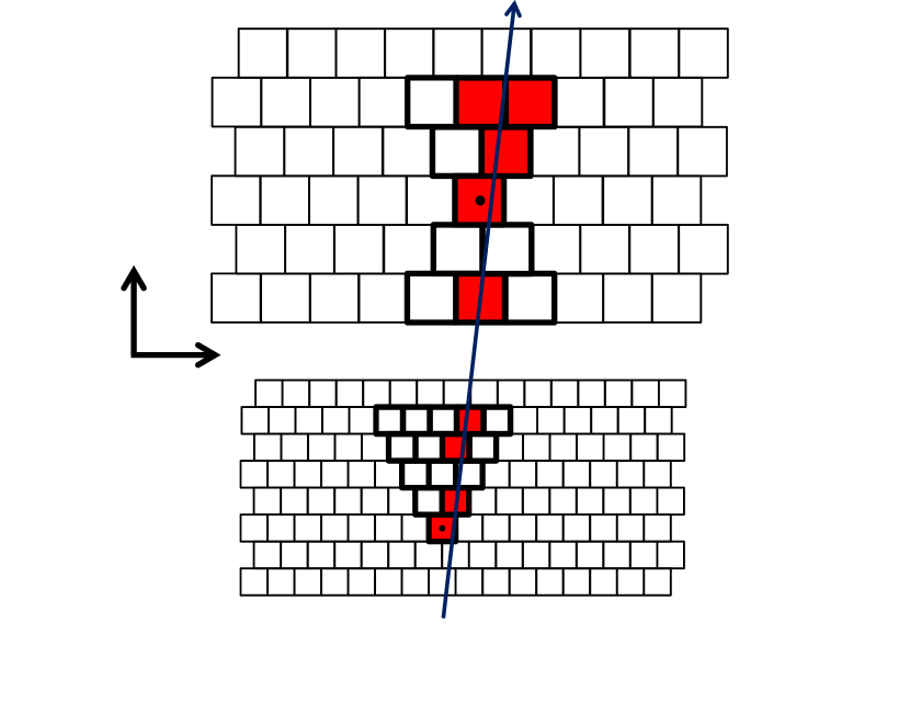
Figure 3: A TS consisting of 5 layers in an SL. The priority wire is indicated by a dot. Top: one of SL 2–9 with the hourglass-shape, bottom: the innermost SL 1 with a different shape and smaller drift cell size.

The neural trigger is operating in parallel to the 3D trigger and fulfills the same task, but with a new multivariate algorithm, providing an independent estimate for the $z$-vertex. Since neural networks are general function approximators capable of learning nonlinear dependencies, they enable a stable 3D track reconstruction also in the presence of noise [3] and inhomogeneities in the electrical (drift) and magnetic (solenoid) fields. Compared to statistical optimal tracking methods used in the offline analysis (e.g. Kalman filter), which are too slow for the use in an online trigger, neural networks provide a good tradeoff between execution speed and prediction accuracy. The outputs of the 2D/3D triggers and the neural network are finally fed into the Global Decision Logic (see Fig. 2).

II-D Planned hardware solution

The data transmission between the individual subsystems of the CDC trigger is carried out via optical links with high speed serial transceivers. Fig. 4 illustrates how the neural network trigger is connected to other trigger components. The hardware system of the neural trigger consists of four FPGA boards, each covering $180^{\circ}$ in the $r-\phi$ plane and having $90^{\circ}$ overlap with its neighbors. Each neural board is connected to four stereo TSF boards, one 2D trigger board and one event timing board. Based on the system real-time requirements and the resulting throughput calculation, the TSF boards deliver an aggregate data bandwidth of $57.024\,\mathrm{Gbps}$, while the data bandwidths coming from the 2D trigger board and the event timing board add up to $23.781\,\mathrm{Gbps}$ and $6.509\,\mathrm{Gbps}$, respectively. Taking into account that a single GTH lane has an actual data rate of $10.160\,\mathrm{Gbps}$, each neural board will require 12 GTH channels for data input (2 GTH per TSF board, 3 GTH for the 2D trigger board and 1 GTH for the event timing board). Two additional GTH channels are reserved for data output to the GDL.

The envisaged hardware solution for the CDC $z$-vertex trigger is based on the Xilinx FPGA VC709 Connectivity Kit. It is equipped with a Xilinx Virtex-7 XC7VX690T FPGA with 3600 dedicated hardware multipliers, which is more than four times the DSP resources available on Virtex-6, its previous generation. This architecture is essential for our method, which requires realtime critical, fully parallelized implementation of neural networks or alternative multivariate methods. Furthermore, this platform features massive high-speed serial I/O capability. There are 4 GTH lanes readily available on the main board. By connecting the Xilinx FM-S18 daughterboard to the FMC connector of the main board, another 10 GTH lanes can be added to the system. With 14 GTH lanes in total, it delivers sufficient I/O bandwidth to communicate with the other trigger components in Belle II which are implemented on UT3 trigger boards [5] developed at KEK. Additionally, it has $8\,\mathrm{GB}$ $1600\,\mathrm{MTs}$ DDR3 memory, which is necessary for the storage and rapid retrieval of the neural network parameters. Extrapolating from our preliminary study with narrow sectors, about $10^{9}$ parameters will be needed ($10^{6}$ MLPs with $10^{3}$ weights each).

This platform is currently the only solution on the market which can fulfill all the requirements on the I/O throughput for the proposed trigger. Having an off-the-shelf platform with rapid prototyping capability enables us to verify and improve our algorithms without excessive amount of investment usually required by customized hardware designs.

Figure 4: Interconnection of the neural board to the other subsystems. One neural board is shown in the figure, together with the bandwidths of data connections to other trigger components. Four neural boards are used in total.

III MLP Prediction

We introduce here the operation principles of the MLP and its application to the $z$-vertex prediction. Each charged track in the detector crosses the magnetic field (1.5 T) parallel to the $z$-direction and can therefore be parametrized by a helix $(p_{T},\phi,d,\theta,z)$, where $p_{T}$ is the transverse momentum, $\phi$ the azimuthal angle at the vertex position, $d$ is the distance of the track to the beam line in the transverse plane ($r-\phi$), $\theta$ is the polar angle with respect to the $z$-axis and $z$ is the position along the beam line. The vertex is considered to be the position of closest approach of the helix to the $z$-axis. The displacement $d$ of background tracks is neglected in our studies, because the main contribution of the expected background tracks is beam induced [4, 5] and thus has $d=0\,\mathrm{cm}$. In addition, background tracks with large displacements in $d$ can be identified and rejected solely by the 2D trigger.

We will show experimental results of MLPs specialized to sectors in the phase space $(p_{T},\phi,\theta,z)$ and trained with Monte Carlo (MC) data, demonstrating the high resolution that can be achieved on the $z$-vertex and confirming results from preliminary studies [1].

III-A MLP structure

Figure 5: Structure of an MLP with one hidden layer. In the nodes the weighted sum of the input values $x_{i}$ is evaluated by the activation function to produce one output value. The weight matrices for the connections are $w_{ji}$ for the input $x_{i}$ to the hidden layer and $w_{kj}$ for the hidden to the output layer. The black nodes denote the constant bias nodes represented by $w_{j0}$ and $w_{k0}$. We scale all input values to the interval $x\in[-1,1]$.

Neural networks are a biologically inspired machine learning model. The MLP is a universal function approximator based on the structure of a directed acyclic graph (see Fig. 5). The intrinsically parallel nature of MLPs is perfectly suited for an implementation on parallel hardware like FPGAs or GPUs. For the 3-layer MLP with one hidden layer, it has been proven that it can approximate any continuous function to any required precision, given a hidden layer of sufficient size and a non-constant, non-linear and bounded activation function [13]. Each neuron computes the weighted sum over its input values and evaluates it with an activation function

$$y_{j}=f\left(\displaystyle\sum_{i=0}^{N}w_{ji}\cdot x_{i}\right)=f(w_{ji}\cdot x_{i})$$ (1)

where the sum in the last term is implicit for double indices. Up to the activation function the calculation for one layer corresponds to a matrix multiplication and can be similarly parallelized, i.e. all neurons are calculated in parallel. The weights $w_{ji}$ contain the information of the calculated function. $y_{j}$ is the output value of neuron $j$, the input vector $x_{i}$ has a constant $x_{0}=1$ to represent a constant bias and the $x_{i},i\in[1..N]$ are the input values. The activation function $f$ is in our case the hyperbolic tangent. The complete function computed by an MLP with hidden nodes $j$ at the output node $k$ is

$$z_{k}=f\left(w_{kj}\cdot f(w_{ji}\cdot x_{i})\right)$$ (2)

where $z_{k}$ are the $k$ outputs of the network, $w_{ji}$ and $w_{kj}$ are the weight matrices connecting the input with the hidden layer ($w_{ji}$) and connecting the hidden with the output layer ($w_{kj}$). The summing over double indices is again implicit. In our setup all input and output values of the MLP are scaled within $[-1,1]$.

III-B MLP training

The training of the MLP is based on a cost function $E$, the mean squared error, applied to the MLP output

$$E=\displaystyle\sum^{N_{\text{train}}}_{i=1}(z_{i}-t_{i})^{2}$$ (3)

where $z_{i}-t_{i}$ is the deviation of the network output $z_{i}$ from the true value $t_{i}$ for the training event $i$ and $N_{\text{train}}$ is the number of training events. In the supervised learning scheme this cost function is minimized by iteratively adjusting the weights in the network proportional to the derivatives

$$\Delta w_{mn}\propto\frac{\partial E}{\partial w_{mn}}$$ (4)

Our network training is performed using the iRPROP^- algorithm [14], an improved variant of the RPROP [15] backpropagation algorithm. This algorithm has been demonstrated to be more effective than the classical backpropagation [16], because the magnitude of the weight update is independent of the magnitude of the derivative of the cost functions and only dependent on the dynamics of the past weight updates. The effect is a faster convergence to a minimum of the cost function with the same minima found as with classical backpropagation [16].

The training procedure can be parallelized by so called “pattern parallel training”, where parallelization is achieved by splitting the set of training patterns over several threads [17]. This is possible because the cost function in (3) is a simple sum over the deviations from the target value for each training pattern. Since all summands are independent from each other, they can be calculated in parallel and then summed up. The same is true for the gradient of the cost function and therefore for the weight updates, which can again be decomposed into a sum of independent terms, each depending on one training pattern.

III-C Sectorization of Input Data

The prediction of the $z$-vertex value with an MLP is possible if the remaining track parameters are known with a sufficient accuracy and thus form a sector in phase space, defined by intervals of the helix track parameters. An “expert” MLP is specialized to a sector by selecting the “relevant” TS that are needed to describe the sector accurately [1]. Only hits from these “relevant” TS are used as input for the MLP. This approach is motivated by [18], where an ensemble of local “experts” is combined with a selection procedure for the optimal local “expert”.

This selection is a necessary preprocessing step to provide a-priori knowledge to the network and to reduce the number of inputs of the MLP to a manageable level. The number of selected “relevant” TS is much smaller than the total number of TS (2336), typically about 1% of the total. Furthermore, it is mainly dominated by the sector sizes in $p_{T}$ and $\phi$, whereas the sector sizes in $\theta$ and $z$ only weakly influence the stereo layers.

For a defined sector in phase space, “relevant” TS can be selected using MC datasets for the Belle II detector. From these datasets a histogram of the TS activity of events within a given sector is generated (see Fig. 6). Small TS ids correspond to the inner layers and large TS ids to the outer SL (e.g. TS id $\in[1,160]$ is SL 1). The 9 peaks correspond to the 9 SL in the CDC and the selection of a small subset of “relevant” TS is obviously justified. On a per SL basis, it is required that a minimum percentage of the hits in all events are found in TS selected as “relevant” within the sector.

Figure 6: Selection of relevant TS in a sector of $\phi\in[180^{\circ},181^{\circ}]$, $\theta\in[35^{\circ},123^{\circ}]$, $p_{T}\in[1.43,1.67]\,\mathrm{GeV}$, $z\in[-50,50]\,\mathrm{cm}$. Each peak corresponds to an SL, alternating between axial and stereo SL. The skewing angle of the stereo SL leads to a broadening of the stereo peaks. The decrease of the peaks towards the outer SL is due to the widening of the sector towards larger radii.

III-D MLP I/O

Once the “relevant” TS for a sector are found, the hits in each event need to be formatted as input for the MLP. While the number of hits in different events can vary, the number of inputs for the MLP needs to be fixed. Two different approaches are used in our studies. The first is a topological input distribution, where each input node corresponds to one relevant TS and the input values are the drift times scaled to the interval $[-1,1]$. Relevant TS that have no hit in a given event are set to a default value corresponding to the maximal drift time, i.e. the track is treated as if it were far away from the TS.

The second approach uses a fixed number of two input nodes per SL, where the first input corresponds to a drift time and the second to a TS id, both scaled to the interval $[-1,1]$. The numbering of the TS within an SL is continuous and can therefore be interpreted as a scaled azimuthal angle. In the rare case that an event has 2 hits in the same SL, the fastest hit is used. In the case that an SL has no hit due to limited efficiency, a default value is used again.

The output of the MLP is also within $[-1,1]$ due to the activation function applied in the output neuron. In order to get a floating point prediction for a helix track parameter, the output is scaled to the sector interval of that variable. While an MLP can generally be trained to predict all track parameters, we use it only to predict the $z$-vertex and the polar angle $\theta$ in our experiments.

III-E “Expert” MLP results for small sectors

Figure 7: Achieved $z$-vertex resolution with MLPs for charged single track events in a small sector constrained by the track parameters $\phi\in[180^{\circ},181^{\circ}]$, $\theta\in[56^{\circ},62^{\circ}]$, $z\in[-10,10]\,\mathrm{cm}$. Top plot: low momentum tracks with transverse momentum $p_{T}\in[0.500,0.513]\,\mathrm{GeV}$, bottom plot: high momentum tracks with $p_{T}\in[4.0,5.0]\,\mathrm{GeV}$.

In order to show that a sufficiently precise $z$-vertex reconstruction is possible at L1, we have tested the MLP approach on single simulated muon tracks from narrow regions in polar and azimuthal angle ($\theta$ and $\phi$), as well as in a limited region of transverse momentum ($p_{T}$). This setup allows to test single sectors without first training all $10^{6}$ MLPs. In the actual trigger the charged tracks in an event will be separated by the 2D finder, so the neural trigger will handle tracks one by one. Training runs in various sectors showed that the required $z$-vertex resolution can indeed be achieved by this method [1]. The results for two different $p_{T}$ regions for a single “expert” MLP (see Fig. 7) show that the $z$-resolutions with $\mathrm{RMS}=1.72\,\mathrm{cm}$ for the low $p_{T}$ case and $\mathrm{RMS}=1.44\,\mathrm{cm}$ for the high $p_{T}$ case are well below our anticipated $2\,\mathrm{cm}$ resolution. A fixed-point implementation suitable for FPGAs has also been carried out and compared to the floating point reference design. There is no evidence of deteriorated $z$-resolutions with $\mathrm{RMS}=1.73\,\mathrm{cm}$ for the low $p_{T}$ case and $\mathrm{RMS}=1.44\,\mathrm{cm}$ for the high $p_{T}$ case.

A preliminary study with post synthesis simulation shows that the execution time of an MLP with 1260 nodes (20 input neurons, 60 hidden neurons, 1 output neuron) is $136\,\mathrm{ns}$. Based on the data throughput of the external memory on our hardware platform, the transfer time for network parameters is estimated to be $223\,\mathrm{ns}$. For the aforementioned network size and topology, the total latency of each processing cycle will be under $400\,\mathrm{ns}$. The latency is linearly proportional to the number of nodes in the MLP.

Note that the sector size in $p_{T}$ needs to be much smaller for the low $p_{T}$ case in order to achieve a comparable resolution for both cases. This is because the geometrically relevant property of the sector, namely the curvature of the track, is proportional to $p_{T}^{-1}$. The two sectors were therefore chosen to have the same size in $\Delta p_{T}^{-1}$ rather than in $\Delta p_{T}$. In the experiment a Geant4 based detector simulation of the Belle II CDC is used. It includes the simulation of physics effects due to material interactions with the inner detector components, the non-linear $x-t$ relation [5] of drift lengths to drift times due to inhomogeneities of the electric field and the wire-sag effect caused by gravitation. With the more realistic physics simulation, the $\mathrm{RMS}$ shown in Fig. 7 is about one third higher than the results achieved in the preliminary studies [1, 2, 3], where an idealized perfect detector was assumed using an older version of the simulation software of the Belle II detector. The non-linear $x-t$ relation has the strongest effect on the $\mathrm{RMS}$.

The generalization of this proof of concept to the full acceptance region of the detector requires a pre-processing that can select the correct sector for each track in the event. The correct selection of the sector is discussed in the next section.

IV Preprocessing

We plan to run the full $z$-vertex trigger system for the Belle II detector as a two step prediction chain: At first the preprocessing step provides the correct sector for an “expert” MLP. Secondly, the “expert” MLP can provide the $z$-vertex as demonstrated in the last section. The experiments detailed in the following section show that the MLP is also a promising candidate for the preprocessing when combined with information from the 2D trigger.

IV-A Finding Sectors

The finding of a sufficiently small sector is crucial for the proper capability of an “expert” MLP to provide high accuracy $z$-vertex predictions. The binning size in the phase space variables is limited by the resolution of the sector finders. For wrongly identified sectors the “expert” networks will fail because the true result is out of range of their specification, which makes the misclassification rate an interesting observable.

As input to the neural network preprocessing, the 2D trigger provides information on the number of tracks in the event and for each track a prediction of $\phi$ and $p_{T}$, based on the active TS and drift times in the axial layers. The appropriate sectors in the $p_{T}-\phi$ space will be provided by the 2D trigger. However, it is not yet clear whether the 2D trigger can yield the required resolution.

As stated before, the number of relevant TS depends mainly on $\phi$ and $p_{T}$ (see section III-C), so with the information of the 2D trigger alone the number of relevant TS can be reduced to a level suitable for the application of an MLP. This first MLP is trained to predict $\theta$ and $z$. It does not reach the final $z$-resolution of $2\,\mathrm{cm}$ as the “expert” MLP, but it is suitable as a preprocessing step. The prediction of the “preprocessing” MLP for $z$ and $\theta$, together with the estimate of $p_{T}$ and $\phi$ provided by the 2D trigger, is then used to select an “expert” MLP which has limited ranges in all track parameters.

Figure 8: Data flow in the prediction chain: the $p_{T}$ and $\phi$ information obtained from the 2D Trigger is enriched with $\theta$ and $z$ information by the preprocessing. This allows selection of an adequate “expert” MLP for the precise $z$-vertex prediction. The MLP approach is also a promising candidate for the Preprocessing.

The workflow of this two step prediction concept is illustrated in Fig. 8. After one preprocessing step ($1^{\text{st}}$ round) the correct “expert” network ($2^{\text{nd}}$ round) is chosen. Our concept can be extended to several steps if necessary. In case the prediction of the “preprocessing” MLP is not precise enough to select a small “expert” MLP, the preprocessing step can again be divided into several steps with successively decreasing sector sizes. In the following we describe an experiment with 3 consecutive steps, where the final step achieved the required $z$-resolution. Whether the required resolution can also be achieved within only two steps will be determined by future research.

IV-B Experimental setup

To demonstrate the capabilities of the prediction chain we use again single simulated muon tracks restricted to a sector in phase space. We started from a sector limited in 2D to $\phi\in[180^{\circ},181^{\circ}]$ and $p_{T}\in[1.43,1.67]\,\mathrm{GeV}$. For the polar angle $\theta$ we chose the starting ranges $[35^{\circ},123^{\circ}]$, which corresponds to the region for which straight tracks coming from the interaction point pass all 9 SL of the CDC. For $z$ the starting range was chosen as $[-50,50]\,\mathrm{cm}$. Within these ranges single tracks were simulated and used to train two MLPs, one with topological input distribution, the other with TS ids as additional input nodes. Both MLPs are trained to predict $z$ and $\theta$. For the selection of the next sector the predictions of both MLPs are averaged, since the combined prediction reaches a better resolution than each MLP alone. The use of a mixture of different “experts” specialized to the same phase space sector is inspired by [19], where a more elaborate combination procedure is proposed (GASEN algorithm).

After testing the resolution of the first step, we define a set of sectors for the second steps based on the measured resolution. For the $z$-vertex the new ranges are determined such that 99 % of the events from $z\in[-1,1]\,\mathrm{cm}$, i.e. possibly interesting physics events, are predicted within the narrowed ranges. Any events predicted outside of the new sector can be safely rejected already in the first step. The $\theta$-resolution is then tested with events from the narrowed $z$-ranges and the $\mathrm{RMS}$ of the difference between true and predicted $\theta$ is calculated. A set of sectors is defined with sector sizes of ${6\cdot\mathrm{RMS}(\theta)}$, which corresponds to a $3\sigma$ interval in both directions. In order to avoid binning effects the sectorization is done with an overlap. With two overlapping binnings, displaced by a half binsize relative to each other, predictions close to the sector border find another sector where they are close to the center.

Figure 9: Resolution of $\theta$ depending on $\theta$ for an MLP with topological input distribution (top) and an MLP with TS ids as additional input nodes (bottom).

The same procedure is repeated to define the sectors for the third step. For each sector we train again one MLP with topological input distribution and one with TS ids as additional input nodes to predict $z$ and $\theta$. For the test of the second step the MLPs of the first step are used to select the sector in $\theta$, i.e. the measured resolution already includes events that were predicted in the wrong sector. Finally the resolution of the third step is measured, again using the first two steps to find the correct sector.

IV-C Prediction of the polar angle $\theta$

The $\theta$-resolution of the preprocessing is of special interest because the performance of the “expert” MLP depends strongly on the sector size in $\theta$. The results for both MLPs of the first step are shown in Fig. 9. The MLP with topological input reaches a different resolution for different $\theta$-regions, while the MLP with TS ids as additional inputs does not depend strongly on $\theta$. On average, the topological MLP reaches a resolution of $\mathrm{RMS}(\theta)=5.8^{\circ}$, the MLP with TS ids reaches a resolution of $\mathrm{RMS}(\theta)=5.2^{\circ}$ and the combined prediction reaches a resolution of $\mathrm{RMS}(\theta)=5.1^{\circ}$. For the second step the sector size in $\theta$ is therefore set to $6\cdot\mathrm{RMS}(\theta)=30.5^{\circ}$.

Figure 10: Sector sizes in $z$ (top) and $\theta$ (bottom) for a prediction chain with 3 steps. The $z$-ranges are iteratively decreased. The $\theta$-ranges in step 2 and 3 are covered with overlapping sectors of decreasing width. The selected sector shown in the figure is an example for an event from $\theta\approx 80^{\circ}$.

IV-D Three step prediction chain

The sector sizes of the prediction chain with 3 consecutive steps of MLPs are visualized in Figure 10. In the first step the combined prediction of the MLP with topological input distribution and the MLP with TS ids as additional input nodes reaches a $z$-resolution of $6.6\,\mathrm{cm}$ and a $\theta$-resolution of $5.1^{\circ}$. Accordingly, the sector size in $\theta$ is set to $30.5^{\circ}$ for the second step, leading to a total number of 7 overlapping sectors. The $z$-ranges for the second step are set to $[-15,15]\,\mathrm{cm}$, in accordance with the requirement that at most 1 % of the events from the interaction region are predicted outside of the new ranges.

In the second step the combined prediction reaches a $z$-resolution of $3.2\,\mathrm{cm}$ and a $\theta$-resolution of $2.8^{\circ}$, with 0.7 % of the test events predicted in the wrong $\theta$-sector. The sector size in $\theta$ is set to $17.0^{\circ}$ for the third and last step, leading to a total of 13 overlapping sectors. The $z$-ranges for the third step are set to $[-8,8]\,\mathrm{cm}$.

The combined prediction of the third step finally reaches a $z$-resolution of $1.7\,\mathrm{cm}$ and a $\theta$-resolution of $1.7^{\circ}$, with 1 % of the test events predicted in the wrong $\theta$-sector. The test proves that the required $z$-resolution can be achieved with our concept, starting from a sector with only 2D information and predicting $z$ and $\theta$.

IV-E Efficiency Analysis

A good way to illustrate the capabilities of the sector prediction methods is to look at their Receiver Operating Characteristic (ROC), which is the true positive rate or efficiency $\varepsilon$ vs. the false positive rate $r_{\mathrm{FP}}$ (background contamination), where “positives” are events predicted within a certain range $[-z_{\text{cut}},z_{\text{cut}}]$ on the $z$-axis. True positives would be physics events from the interaction region ($z=0\,\mathrm{cm}$) predicted in these ranges, while false positives are background events predicted in these ranges. Since we are working with simulated single tracks rather than real events, we define all tracks within $z\in[-1,1]\,\mathrm{cm}$ as potentially interesting events (see Table I). The efficiency $\varepsilon$ and contamination $r_{\mathrm{FP}}$ are then defined as

TABLE I: Definitions for the Receiver Operating Characteristic

	$z_{\text{true}}\in[-1,1]\,\mathrm{cm}$	$z_{\text{true}}\notin[-1,1]\,\mathrm{cm}$
$z_{\text{pred}}\in[-z_{\text{cut}},z_{\text{cut}}]$	TP	FP
$z_{\text{pred}}\notin[-z_{\text{cut}},z_{\text{cut}}]$	FN	TN

TP: True Positives, FP: False Positives,
FN: False Negatives, TN: True Negatives,
$z_{\text{true}}$: true $z$-vertex provided by the simulation,
$z_{\text{pred}}$: prediction of the neural network

Figure 11: ROC for $z$ for 3 steps of the prediction chain. The Area Under the Curve (AUC) is a measure for the quality of the predictor, where a perfect predictor would have an AUC of 1.

$$\varepsilon=\frac{\text{TP}}{\text{TP}+\text{FN}}; r_{\mathrm{FP}}=\frac{\text{FP}}{\text{FP}+\text{TN}}$$ (5)

The parameter $z_{\text{cut}}$ is varied to generate different values for the efficiency and the contamination. The resulting ROC curves for the 3 training steps are shown in Fig. 11. The improvement of the prediction with each new step is clearly visible. With a cut at $z_{\text{cut}}=6\,\mathrm{cm}$ a contamination of 17.1% can be obtained while keeping an efficiency of 98.2%. Note that the background contamination contains events outside of the interesting region of $[-1,1]\,\mathrm{cm}$, but within the cut interval of $[-6,6]\,\mathrm{cm}$, i.e. an MLP with perfect prediction would still have a false positive rate of 10.2% at this cut value. The real background rejection in the experiment will depend on the topological distribution of the background tracks, for which the study has just been started.

V Conclusion

We have presented the concept for a first level $z$-vertex trigger for the Belle II experiment, using the hit information from the CDC without explicit track reconstruction. The concept is based on an ensemble of “expert” MLPs, specialized to sectors in phase space, defined by $\phi,\theta$ and $p_{T}$, which are small enough to contain single tracks. Using the $p_{T}$ and $\phi$ information from the standard CDC 2D trigger, MLPs are used in a preprocessing step to roughly estimate the polar angle $\theta$ and the $z$-vertex for each track. Then the pre-trained expert MLPs determine the $z$-vertices of the tracks. Based on our preliminary investigations, the current state-of-the-art hardware is able to provide sufficient computing resources to implement the large number of “expert” neural networks. In the near future we will explore the optimal full prediction chain and provide measurements with the hardware. To this end, new algorithms for the sector finding will be explored. Especially, the proper combination of different predictors in each preprocessing step will be optimized. Then MLPs will be trained for all sectors and the neural trigger will be tested with full events. The $z$-vertices of several tracks will be estimated separately and combined to improve the prediction for the full event. After a successful completion of the studies, the plan is to install the neural network trigger into the Belle II trigger system.

While the presented methods are developed and tested primarily for the Belle II experiment, the concept could also be applied for the development of other track-based trigger algorithms. The proposed method could be useful for the LHC experiments in the muon trigger area, estimating e.g. the muon transverse momentum. For the future generations of silicon detectors it could also be used as a secondary vertex trigger. The method could even be used for a fast online track reconstruction using, e.g. the straw tube trackers of the Panda experiment at FAIR [20]. Furthermore, the combination of a preprocessing step with sectorized local experts is a very general divide and conquer approach that can also be transferred to various other problems.

References

- [1] S. Skambraks, “Use of Neural Networks for Triggering in Particle Physics,” Diplomarbeit, Inst. for Informatics, Ludwig-Maximilians-Univ., München, 2013. [Online]. Available: https://publications.mppmu.mpg.de/2013/MPP-2013-339/FullText.pdf
- [2] S. Skambraks, “Use of Neural Networks for Triggering in the Belle II Experiment,” M.S. thesis, Faculty of Physics, Ludwig-Maximilians-Univ., München, 2013. [Online]. Available: https://publications.mppmu.mpg.de/2013/MPP-2013-377/FullText.pdf
- [3] F. Abudinén, “Studies on the neural -Vertex-Trigger for the Belle II Particle Detector,” M.S. thesis, Faculty of Physics, Ludwig-Maximilians-Univ., München, 2014. [Online]. Available: https://publications.mppmu.mpg.de/2014/MPP-2014-42/FullText.pdf
- [4] Y. Iwasaki et al., “Level 1 Trigger System for the Belle II Experiment,” IEEE Trans. Nucl. Sc., vol. 58, no. 4, pp. 1807–1815, Aug. 2011.
- [5] T. Abe et al., “Belle II Technical Design Report,” Nov. 2010. [Online]. Available: http://arxiv.org/abs/1011.0352
- [6] S. Hashimoto et al., “LoI for KEK Super B Factory, Part I: Physics,” 2004. [Online]. Available: http://superb.kek.jp/documents/loi/img/LoI_physics.pdf
- [7] T. Aushev, W. Bartel, A. Bondar, J. Brodzicka, T. Browder et al., “Physics at Super B Factory,” 2010. [Online]. Available: http://arxiv.org/abs/1002.5012
- [8] A. Abashian et al., “The Belle detector,” Nucl. Instrum. Methods A, vol. 479, no. 1, pp. 117–232, 2002.
- [9] B. Aubert et al., “The BABAR detector,” Nucl. Instrum. Methods A, vol. 479, no. 1, pp. 1–116, 2002.
- [10] C. Bernardini et al., “Lifetime and Beam Size in a Storage Ring,” Phys. Rev. Lett., vol. 10, pp. 407–409, May 1963.
- [11] A. Piwinski, “The Touschek Effect in Strong Focusing Storage Rings,” 1998. [Online]. Available: http://arxiv.org/abs/physics/9903034
- [12] S. Bailey et al., “Rapid 3D track reconstruction with the BaBar trigger upgrade,” Nucl. Instrum. Methods A, vol. 518, no. 1-2, pp. 544–548, 2004.
- [13] R. Hecht-Nielsen, “Theory of the backpropagation neural network,” in 1989 IJCNN, IEEE Int. Joint Conf. Neural Networks, vol. 1, pp. 593–605.
- [14] C. Igel and M. Hüsken, “Improving the Rprop Learning Algorithm,” in Proc. 2nd Int. Symp. Neural Computation, 2000, pp. 115–121.
- [15] M. Riedmiller and H. Braun, “A direct adaptive method for faster backpropagation learning: the RPROP algorithm,” in 1993 IEEE Int. Conf. Neural Networks, vol. 1, pp. 586–591.
- [16] C. Igel and M. Hüsken, “Empirical evaluation of the improved Rprop learning algorithms,” Neurocomputing, vol. 50, pp. 105–123, 2003.
- [17] G. Dahl, A. McAvinney, and T. Newhall, “Parallelizing Neural Network Training for Cluster Systems,” in Proc. IASTED, Int. Conf. on Parallel and Distributed Computing and Networks, ser. PDCN ’08. Anaheim, CA, USA: ACTA Press, 2008, pp. 220–225.
- [18] R. A. Jacobs, M. I. Jordan, S. J. Nowlan, and G. E. Hinton, “Adaptive Mixtures of Local Experts,” Neural Compution, vol. 3, no. 1, pp. 79–87, Mar. 1991.
- [19] Z.-H. Zhou, J. Wu, and W. Tang, “Ensembling neural networks: Many could be better than all,” Artificial Intelligence, vol. 137, no. 1-2, pp. 239–263, 2002.
- [20] W. Erni et al., “Technical design report for the PANDA (AntiProton Annihilations at Darmstadt) Straw Tube Tracker,” Eur. Phys. J. A, vol. 49, no. 2, 2013.