A non-equilibrium equation-of-motion approach to quantum transport utilizing projection operators

Abstract

We consider a projection operator approach to the non-equilbrium Green function equation-of-motion (PO-NEGF EOM) method. The technique resolves problems of arbitrariness in truncation of an infinite chain of EOMs, and prevents violation of symmetry relations resulting from the truncation. The approach, originally developed by Tserkovnikov [Theor. Math. Phys. 118, 85 (1999)] for equilibrium systems, is reformulated to be applicable to time-dependent non-equilibrium situations. We derive a canonical form of EOMs, thus explicitly demonstrating a proper result for the non-equilibrium atomic limit in junction problems. A simple practical scheme applicable to quantum transport simulations is formulated. We perform numerical simulations within simple models, and compare results of the approach to other techniques, and (where available) also to exact results.

I Introduction

Since the first theoretical prediction of the possibility to utilize molecules as active elements in junctions,Aviram and Ratner (1974) molecular electronics has been driven by developments in experimental abilities to fabricate and control molecular nanostructures. Inelastic electron tunneling spectroscopy (IETS),Galperin et al. (2008a, 2007a) molecular optoelectronics,Galperin and Nitzan (2012) molecular nanoplasmonics,Chen et al. (2012) and molecular spintronicsSanvito and Rocha (2006); Bogani and Wernsdorfer (2008); Wernsdorfer (2010); Sanvito (2011); Naaman and Waldeck (2012) are branches of molecular electronics, where experimental data require development of an adequate theoretical techniques.

Resonant IETS with its strong electron-vibration coupling and anharmonic effects,Park et al. (2000) as well as observation of breakdown of the Born-Oppenheimer approximation,Repp et al. (2010) requires formulation in the basis of vibronic states.Bonca and Trugman (1995); White and Galperin (2012) Similarly, in optoelectronic devices, where covalent bonding between molecule and contacts results in hybridization between molecular excitation and plasmon resonances,Esteban et al. (2012) separation into electronic and plasmonic degrees of freedom is inadequate.White et al. (2012) Finally, physics of single molecule magnet devices is achieved most conveniently by diagonalizing the multi-spin Hamiltonian.Jo et al. (2006); Quddusi et al. (2011)

Development of theoretical methods capable of describing transport in molecular junctions in the language of many-body states of an isolated system - the nonequilibrium atomic limit - is necessary for adequate description in the situations similar to those mentioned above.White et al. (2014a) Examples of such formulations include scattering theory methods,Bonca and Trugman (1995); Haule and Bonca (1999); Emberly and Kirczenow (2000); Jorn and Seideman (2010); Galperin and Nitzan (2013) quantum master equation approaches,Koch and von Oppen (2005); Koch et al. (2006); Siddiqui et al. (2007); Leijnse and Wegewijs (2008); Esposito and Galperin (2009, 2010); Zelinskyy and May (2012); Saptsov and Wegewijs (2012) pseudoparticleEckstein and Werner (2010); Oh et al. (2011); White and Galperin (2012); White et al. (2012); Marbach et al. (2012); White et al. (2013, 2014b) and HubbardSandalov et al. (2003); Fransson (2005); Sandalov and Nazmitdinov (2007); Galperin et al. (2008b); Yeganeh et al. (2009) non-equilibrium Green function techniques.

A simple general alternative is the equation-of-motion (EOM) methodBonch-Bruevich and Tyablikov (1962); Kadanoff and Baym (1962) formulated for transport problems on the Keldysh contour.Bulka and Kostyrko (2004); Kostyrko and Bułka (2005); Špička et al. (2005); Galperin et al. (2006); Galperin et al. (2007b); Trocha and Barnaś (2008); Świrkowicz et al. (2009); Fainberg et al. (2011); Levy and Rabani (2013a); Levy and Rabani (2013b) EOM permits working with correlation functions of any operators to produce (in general) an infinite chain of equations of motion. The main drawback of the method is the necessity to make an uncontrolled approximation to close the chain of equations. Usually, a justification for such an approximation can be obtained only a posteriori. Moreover, uncontrolled decoupling of correlation functions may result in complications related to loss of proper commutation relations between the decoupled operators.Bonch-Bruevich and Tyablikov (1962) Violation of symmetry relations due to such an uncontrolled decoupling in quantum transport problems was discussed in Refs. Levy and Rabani, 2013a; Levy and Rabani, 2013b.

Projection operators are often employed to derive an exact quantum master equation (QME) for a system coupled to baths.Zwanzig (2001); Breuer and Petruccione (2003); Nitzan (2006); van Kampen (2007); van Vliet and Vasilopoulos (1988); Koide (2002); Michel et al. (2007); Gemmer and Breuer (2007); Steinigeweg et al. (2009) In the theory of equilibrium Green functions, projection techniques are sometimes utilized to close the chain of EOMs.Roth (1968); Ichiyanagi (1972); Goryachev et al. (1982); Ruckenstein and Schmitt-Rink (1989) In particular, an approach developed by TserkovnikovTserkovnikov (1981, 1999) guarantees that truncating an infinite chain of equations at step $n$ includes correlations between the originally chosen set of operators to order $n$. The approach was shown to be equivalent to Mori’s methodMori (1965); Ryu and Choi (1991); Okada et al. (1995) employed in QME derivations.

Here we formulate the approach of Refs. Tserkovnikov, 1981, 1999; Plakida, 2011 on the Keldysh contour, and discuss its applicability to transport problems. In particular, we demonstrate that the approach permits a formulation of a symmetrized Dyson-type equation which by construction resolves symmetry violations discussed in Refs. Levy and Rabani, 2013a; Levy and Rabani, 2013b. Also we argue that the approach resolves the problems of the first Hubbard (HIA) approximation related to Hermiticity of a resulting reduced density matrix.Galperin et al. (2008b); Pedersen et al. (2009)

After introducing the generalization of the scheme in Section IIA, in Section IIB we derive a Dyson-type EOM for effective canonical quasi-particles, which is crucial for construction of a proper diagrammatic expansion.Shastry (2010) Then in Section IIC we discuss application of the resulting scheme to transport in junctions. Section III presents numerical results. Section IV concludes.

II Method

We start by generalizing the scheme of Refs. Tserkovnikov, 1981, 1999; Plakida, 2011 to the realm of open quantum systems far from equilibrium in Section II.1. General consideration follows by derivation of the EOM for canonical Green function in Section II.2. Finally, in Section II.3 we discuss application of the scheme to transport in junctions.

II.1 EOM for irreducible Green functions

Following Ref. Tserkovnikov, 1999 we start by introducing a column vector operator $\hat{a}_{1}$. Both choice and number $M_{1}$ of its elements depend on the particular problem (see Section III for examples). This flexibility of choice is an advantage, allowing to greatly simplify solution once the initial vector-operator is taken according to physics of a problem (see examples in Section III). The moment the original operator has been chosen the methodology provides a tool for taking account of correlations between the operators in an ordered fashion.

EOMs (in the Heisenberg picture) for this vector-operator and its Hermitian conjugate are (here and below $\hbar=1$)

$$i\frac{\partial}{\partial\tau}\hat{a}_{n}(\tau)\equiv \left[\hat{a}_{n};\hat{H}\right](\tau)$$ (1)

$$=\mathbf{\varepsilon}_{n}(\tau)\hat{a}_{n}(\tau)+\mathbf{\nu}_{n,n+1}(\tau)\hat{a}_{n+1}(\tau),$$

$$-i\frac{\partial}{\partial\tau^{\prime}}\hat{a}_{n}^{\dagger}(\tau^{\prime})\equiv \left[\hat{H};\hat{a}_{n}^{\dagger}\right](\tau^{\prime})$$ (2)

$$=\hat{a}_{n}^{\dagger}(\tau^{\prime})\bar{\mathbf{\varepsilon}}_{n}(\tau^{\prime})+\hat{a}_{n+1}^{\dagger}(\tau^{\prime})\mathbf{\nu}_{n+1,n}(\tau^{\prime}).$$

Here $n=1,2,3,\ldots$ is the index for the infinite sequence of operators defined by the EOMs (1) and (2), $\tau$ and $\tau^{\prime}$ are contour variables, and $\hat{H}$ is the total Hamiltonian. $\mathbf{\varepsilon}_{n}$ and $\mathbf{\nu}_{n,n+1}$ are matrices of size $M_{n}\times M_{n}$ and $M_{n}\times M_{n+1}$, respectively, defined by commutation of operators constituting vector the $\hat{a}_{n}$ with the Hamiltonian $\hat{H}$. $\bar{\mathbf{\varepsilon}}_{n}=\mathbf{\varepsilon}_{n}^{\dagger}$ and $\mathbf{\nu}_{n+1,n}=\mathbf{\nu}_{n,n+1}^{\dagger}$. Note that $\hat{a}_{n}^{\dagger}$ is a row vector operator with elements being Hermitian conjugates of those in $\hat{a}_{n}$. Here and below $\mathbf{\varepsilon}_{n}(\tau)$ indicates values of the matrix at physical time $t$ corresponding to contour variable $\tau$ (and similar for other matrices). Such dependence appears when the Hamiltonian contains a time-dependent process.

The scalar product $\mathbf{P}_{a,b}$ of two arbitrary vector operators $\hat{a}$ and $\hat{b}$ is defined as an average over a non-equlibrium state of a commutator (if at least one of the vectors is of Bose type) or an anti-commutator (if both operators are of Fermi type)

$$\mathbf{P}_{a,b}\equiv\left\langle\left[\hat{a};\hat{b}^{\dagger}\right]_{\pm}\right\rangle.$$ (3)

Note that $\mathbf{P}_{a,b}$ is a matrix of size $M_{a}\times M_{b}$.

Utilizing this definition of scalar product, Eq.(3), we next introduce orthogonalized vector operators

$$\hat{A}_{n}\equiv \hat{a}_{n}-\sum_{i=1}^{n-1}\mathbf{P}_{a_{n},A_{i}}\,\mathbf{P}_{A_{i},A_{i}}^{-1}\,\hat{A}_{i}$$ (4)

$$\hat{A}_{n}^{\dagger}\equiv \hat{a}_{n}^{\dagger}-\sum_{i=1}^{n-1}\hat{A}_{i}^{\dagger}\,\mathbf{P}_{A_{i},A_{i}}^{-1}\,\mathbf{P}_{A_{i},a_{n}}$$ (5)

where $\hat{A}_{1}\equiv\hat{a}_{1}$. Here and below we use capital letters for orthogonalized vector operators. Note that in Eqs. (4) and (5), as well as below, we assume existence of inverse of the spectral weight matrix, Eq.(3). While this property cannot be guaranteed in general, it can be proven for Fermi type excitations in a system held at finite temperature (see Appendix A). These are the conditions of main interest for quantum transport problems in junctions, and this is the situation we consider in the paper.

Our goal is to evaluate the non-equilibrium Green function of the operators of interest $\hat{a}_{1}$

$$\mathbf{G}_{a_{1},a_{1}}(\tau,\tau^{\prime})\equiv-i\left\langle T_{c}\,\hat{a}_{1}(\tau)\,\hat{a}_{1}^{\dagger}(\tau^{\prime})\right\rangle,$$ (6)

where $T_{c}$ is the contour ordering operator and $\mathbf{G}$ is $M_{1}\times M_{1}$ matrix. For future reference it is convenient to introduce irreducible Green functions

$$\mathbf{G}^{(n)}_{a,b}(\tau,\tau^{\prime})\equiv\mathbf{G}^{(n-1)}_{a,b}(\tau,\tau^{\prime})$$ (7)

$$-\int_{c}d\tau_{1}\int_{c}d\tau_{2}\mathbf{G}^{(n-1)}_{a,A_{n}}(\tau,\tau_{1})\hat{\mathbf{G}}^{-1\,(n-1)}_{A_{n},A_{n}}(\tau_{1},\tau_{2})\mathbf{G}^{(n-1)}_{A_{n},b}(\tau_{2},\tau^{\prime})$$

Here integration is over the Keldysh contour, $\mathbf{G}^{(0)}_{a,b}(\tau,\tau^{\prime})\equiv\mathbf{G}_{a,b}(\tau,\tau^{\prime})$, and $\hat{\mathbf{G}}^{-1\,(n-1)}_{A_{n},A_{n}}(\tau_{1},\tau_{2})$ is the inverse operator for the irreducible Green function $\mathbf{G}^{(n-1)}_{A_{n},A_{n}}(\tau_{1},\tau_{2})$

$$\int_{c}d\tau_{1}\hat{\mathbf{G}}^{-1\,(n-1)}_{A_{n},A_{n}}(\tau,\tau_{1})\,\mathbf{G}^{(n-1)}_{A_{n},A_{n}}(\tau_{1},\tau^{\prime})=$$ (8)

$$\int_{c}d\tau_{1}\mathbf{G}^{(n-1)}_{A_{n},A_{n}}(\tau,\tau_{1})\,\hat{\mathbf{G}}^{-1\,(n-1)}_{A_{n},A_{n}}(\tau_{1},\tau^{\prime})=\delta(\tau,\tau^{\prime})\,\mathbf{I}_{n}$$

where $\mathbf{I}_{n}$ is the $M_{n}\times M_{n}$ unit matrix. Considering Eq.(6) as a scalar product in an extended Hilbert space (the one including the contour variable as part of the index), definition of irreducible Green functions in Eq.(7) is similar to projection in Eqs. (4) and (5), where each next generation of correlation functions is orthogonalized relative to the previous one. This definition provides properties which eventually lead to formulation of a canonical Dyson-type equation (see Eq.(14) below). Note that this result would be impossible without the orthogonalization introduced in Eq.(7).

In terms of the irreducible Green functions, Eq.(7), the chain of (left and right) EOMs for the Green function (6) is (see Appendix B for derivation)

$$\left[i\frac{\overset{\rightarrow}{\partial}}{\partial\tau}-\mathbf{\omega}_{n}(\tau)\right]\mathbf{G}^{(n-1)}_{A_{n},A_{n}}(\tau,\tau^{\prime})=\delta(\tau,\tau^{\prime})\,\mathbf{P}_{A_{n},A_{n}}(\tau)$$

$$\quad+\int_{c}d\tau_{1}\,\mathbf{P}_{A_{n},A_{n}}(\tau)\,\mathbf{\Sigma}^{(n-1)}_{A_{n},A_{n}}(\tau,\tau_{1})\,\mathbf{G}^{(n-1)}_{A_{n},A_{n}}(\tau_{1},\tau^{\prime})$$ (9)

$$\mathbf{G}^{(n-1)}_{A_{n},A_{n}}(\tau,\tau^{\prime})\left[-i\frac{\overset{\leftarrow}{\partial}}{\partial\tau^{\prime}}-\bar{\mathbf{\omega}}_{n}(\tau^{\prime})\right]=\delta(\tau,\tau^{\prime})\,\mathbf{P}_{A_{n},A_{n}}(\tau)$$

$$\quad+\int_{c}d\tau_{1}\,\mathbf{G}^{(n-1)}_{A_{n},A_{n}}(\tau,\tau_{1})\,\mathbf{\Sigma}^{(n-1)}_{A_{n},A_{n}}(\tau_{1},\tau^{\prime})\,\mathbf{P}_{A_{n},A_{n}}(\tau^{\prime})$$ (10)

where

$$\mathbf{\omega}_{n}(\tau)\equiv \mathbf{\varepsilon}_{n}(\tau)+\mathbf{\nu}_{n,n+1}(\tau)\,\mathbf{P}_{a_{n+1},A_{n}}(\tau)\,\mathbf{P}_{A_{n},A_{n}}^{-1}(\tau)$$

$$-\mathbf{P}_{a_{n},A_{n-1}}(\tau)\,\mathbf{P}_{A_{n-1},A_{n-1}}^{-1}(\tau)\,\mathbf{\nu}_{n-1,n}(\tau)$$ (11)

is a normalized free evolution matrix, $\bar{\mathbf{\omega}}_{n}(\tau)\equiv\mathbf{\omega}_{n}^{\dagger}(\tau)$, and

$$\mathbf{\Sigma}^{(n-1)}_{A_{n},A_{n}}(\tau,\tau^{\prime})\equiv \mathbf{P}_{A_{n},A_{n}}^{-1}(\tau)\,\mathbf{\nu}_{n,n+1}(\tau)\,\mathbf{G}_{A_{n+1},A_{n+1}}^{(n)}(\tau,\tau^{\prime})$$

$$\times\mathbf{\nu}_{n+1,n}(\tau^{\prime})\,\mathbf{P}_{A_{n},A_{n}}^{-1}(\tau^{\prime})$$ (12)

is the irreducible self-energy of the Green function $\mathbf{G}_{A_{n},A_{n}}^{(n-1)}(\tau,\tau^{\prime})$ due to higher order correlations. Eqs. (II.1) and (II.1) complete formulation of the EOM scheme of Refs. Tserkovnikov, 1981, 1999 on the Keldysh contour. This generalization paves a way to application of the scheme to non-equilibrium systems. As expected, the chain of equations (II.1) and (II.1) is usually infinite. However, contrary to the standard EOM scheme, this normalized irreducible formulation guarantees that truncating the chain at step $n$ is equivalent to neglecting higher order correlations only. Note that structure of Eqs. (II.1) and (II.1) for $n=1$ is similar to that of the first Hubbard (HIA) approximation derived for the Hubbard non-equilibrium Green functions (see e.g. Ref. Sandalov and Nazmitdinov, 2007).

Similar to usual EOM techniques each next step takes into account higher correlations induced in the system by coupling (in our case) to baths. Note however that in the standard EOM techniques each next step brings in addition to higher order processes also multiple correlations of the lower order. In the present methodology those are excluded by the orthogonalization procedure. A detailed discussion and graphic representation for equilibrium Green functions EOMs can be found in Ref. Tserkovnikov, 1999.

II.2 EOM for canonical Green functions

While the form of Eqs. (II.1) and (II.1) is suggestively of a Dyson-type, the quasiparticles described by the corresponding Green functions are of a non-canonical nature due to spectral weight $\mathbf{P}_{A_{n},A_{n}}(\tau)$ in the right side of the equations.Shastry (2010) Also left vs. right symmetry is not obvious in the present form of the equations. A local gauge transformation with a space-time factor is needed to achieve canonical form of the expressions. To reveal canonical quasiparticles we choose the following scaling

$$\mathcal{G}^{(n-1)}_{A_{n},A_{n}}(\tau,\tau^{\prime})\equiv\mathbf{P}_{A_{n},A_{n}}^{-1/2}(\tau)\,\mathbf{G}^{(n-1)}_{A_{n},A_{n}}(\tau,\tau^{\prime})\,\mathbf{P}_{A_{n},A_{n}}^{-1/2}(\tau^{\prime})$$ (13)

Applying transformation (13) to the left EOM, Eq. (II.1), leads to an EOM for the canonical Green function

$$\left[i\frac{\overset{\rightarrow}{\partial}}{\partial\tau}-\mathcal{W}_{n}(\tau)\right]\mathcal{G}^{(n-1)}_{A_{n},A_{n}}(\tau,\tau^{\prime})=\delta(\tau,\tau^{\prime})\,\mathbf{I}_{n}$$ (14)

$$\qquad+\int_{c}d\tau_{1}\,\mathcal{S}^{(n-1)}_{A_{n},A_{n}}(\tau,\tau_{1})\,\mathcal{G}^{(n-1)}_{A_{n},A_{n}}(\tau_{1},\tau^{\prime})$$

Here

$$\mathcal{S}^{(n-1)}_{A_{n},A_{n}}(\tau,\tau^{\prime})=\mathbf{P}_{A_{n},A_{n}}^{1/2}(\tau)\,\mathbf{\Sigma}^{(n-1)}_{A_{n},A_{n}}(\tau,\tau^{\prime})\,\mathbf{P}_{A_{n},A_{n}}^{1/2}(\tau^{\prime})$$

$$\quad\equiv\mathcal{N}_{n,n+1}(\tau)\,\mathcal{G}^{(n)}_{A_{n+1},A_{n+1}}(\tau,\tau^{\prime})\,\mathcal{N}_{n+1,n}(\tau^{\prime}),$$ (15)

with

$$\mathcal{N}_{n,n+1}(\tau)\equiv\mathbf{P}_{A_{n},A_{n}}^{-1/2}(\tau)\,\mathbf{\nu}_{n,n+1}(\tau)\,\mathbf{P}_{A_{n+1},A_{n+1}}^{1/2}(\tau)$$ (16)

and $\mathcal{N}_{n+1,n}(\tau)=\mathcal{N}_{n,n+1}^{\dagger}(\tau)$, is the canonical quasiparticle self-energy. To derive the second line in Eq.(II.2) we employed Eqs. (II.1) and (13). The free evolution matrix is (see Appendix C for derivation)

$$\mathcal{W}_{n}(\tau)= \frac{i}{2}\frac{\partial}{\partial\tau}\left[\mathbf{P}_{A_{n},A_{n}}^{1/2}(\tau)\right]\,\mathbf{P}_{A_{n},A_{n}}^{-1/2}(\tau)$$ (17)

$$+ \frac{1}{2}\mathbf{P}_{A_{n},A_{n}}^{-1/2}(\tau)\,\mathbf{\omega}_{n}(\tau)\,\mathbf{P}_{A_{n},A_{n}}^{1/2}(\tau)+H.c.$$

Note that since the free evolution matrix is Hermitian, $\mathcal{W}_{n}(\tau)=\mathcal{W}_{n}^{\dagger}(\tau)$, and the self-energy matrix $\mathcal{S}^{(n-1)}_{A_{n},A_{n}}(\tau,\tau^{\prime})$ is symmetric relative to normalization factors, Eq.(II.2), a similar derivation starting right EOM, Eq.(II.1), leads to the same result. Thus Eq.(14) is of canonical Dyson form. This is the main exact result of our consideration.

Calculations based on the infinite chain of EOMs, Eq.(14), are truncated at some finite step $n$ by an approximation performed on self-energy $\mathcal{S}^{(n-1)}_{A_{n},A_{n}}(\tau,\tau^{\prime})$ of the last equation in the chain. For example, one can completely neglect the self-energy, or assume a decoupling procedure, which will allow expressing the self-energy in terms of Green functions available in the chain. The resulting finite set of equations has to be solved self-consistently, since spectral weights (normalization factors), Eq.(3), can be expressed in terms of Green functions, which they also define (see Eqs. (14)-(17)).

Note that while (similar to the standard EOM methods) truncation of the chain (13) cannot formally guarantee conserving character of the approximation, the methodology described here does resolve two important drawbacks of the usual EOM formulations: 1. Contrary to the usually employed truncation schemes it provides a way to make decoupling controllable in a sense that at each step one takes into account systematically the greater complexity of the correlations; 2. It resolves the symmetry-breaking problem in decoupling chain of Green function EOMs in the sense of left vs. right EOM incompatibility. The latter problem is relevant for EOM formulations for both usualBonch-Bruevich and Tyablikov (1962); Levy and Rabani (2013a); Levy and Rabani (2013b) and HubbardSandalov et al. (2003); Fransson (2005); Sandalov and Nazmitdinov (2007); Galperin et al. (2008b) Green functions, and may lead to complications (for example, non-Hermiticity of the density matrix). In the presented formulation Hermiticity and positive definiteness of the density matrix is guaranteed by the canonical from of Eq.(13) (see Appendix E). Note also that in the examples presented in Section III the approach provides results which do not violate conservation laws. Finally, infinite chain of EOMs (13) is exact, and can be viewed as a way to define proper quasiparticles for strongly interacting molecules in junctions. Note that these quasiparticles are not are not molecular or Kohn-Sham orbitals (even when the latter are obtained from an (unknown) exact pseudopotential).

II.3 Application to transport in junctions

Till now our considerations were exact. However, direct application of the scheme described above to open systems leads to a set of hierarchical EOMs. Each subsequent step in the hierarchy accounts for additional correlations caused by system-bath coupling. The resulting multi-energy correlation functions are similar to those discussed in the literatureJin et al. (2008) with the distinction that in the present consideration the hierarchy is formulated for Green functions rather than for a density matrix. While the scheme is well defined, and in combination with TDDFT may be even practically applicableZheng et al. (2010) (see Section III.1 below), rigorous many-body formulation quickly becomes prohibitively expensive.

A simple approximate practical alternative is based on substitution of the infinite chain of equations, Eq. (14), by the first equation in the chain ($n=1$) with self-energy $\mathcal{S}^{(0)}_{A_{1},A_{1}}(\tau,\tau^{\prime})$ obtained from an approximate self-consistent formulation. We note that the self-energy $\mathcal{S}^{(0)}_{A_{1},A_{1}}(\tau,\tau^{\prime})$ is defined in terms of irreducible Green function $\mathcal{G}_{A_{2},A_{2}}^{(1)}(\tau,\tau^{\prime})$, Eq.(II.2). Then utilizing Eqs. (4), (5), (7), and (8) after lengthy but straightforward transformations we get (see Appendix D for derivation)

$$\mathcal{S}^{(0)}_{A_{1},A_{1}}(\tau,\tau^{\prime})=\mathcal{S}(\tau,\tau^{\prime})-\mathcal{R}(\tau)\,\mathcal{G}^{(0)}_{A_{1},A_{1}}(\tau,\tau^{\prime})\,\mathcal{R}^{\dagger}(\tau^{\prime})$$

$$-\int_{c}d\tau_{1}\bigg{(}\mathcal{R}(\tau)\,\mathcal{G}^{(0)}_{A_{1},A_{1}}(\tau,\tau_{1})\,\mathcal{S}_{A_{1},A_{1}}^{(0)}(\tau_{1},\tau^{\prime})$$

$$\qquad\quad+\mathcal{S}_{A_{1},A_{1}}^{(0)}(\tau,\tau_{1})\,\mathcal{G}^{(0)}_{A_{1},A_{1}}(\tau_{1},\tau^{\prime})\,\mathcal{R}^{\dagger}(\tau^{\prime})\bigg{)}$$ (18)

$$-\int_{c}d\tau_{1}\int_{c}d\tau_{2}\,\mathcal{S}_{A_{1},A_{1}}^{(0)}(\tau,\tau_{1})\,\mathcal{G}^{(0)}_{A_{1},A_{1}}(\tau_{1},\tau_{2})\,\mathcal{S}_{A_{1},A_{1}}^{(0)}(\tau_{2},\tau^{\prime})$$

where

$$\mathcal{S}(\tau,\tau^{\prime})\equiv \mathbf{P}^{-1/2}_{A_{1},A_{1}}(\tau)\,\mathbf{\nu}_{1,2}(\tau)\,\mathbf{G}_{a_{2},a_{2}}(\tau,\tau^{\prime})\,$$ (19)

$$\times\mathbf{\nu}_{2,1}(\tau^{\prime})\,\mathbf{P}_{A_{1},A_{1}}^{-1/2}(\tau^{\prime})$$

$$\mathcal{R}(\tau)\equiv \mathbf{P}_{A_{1},A_{1}}^{-1/2}(\tau)\,\mathbf{\nu}_{1,2}(\tau)\,\mathbf{P}_{a_{2},A_{1}}(\tau)\,\mathbf{P}_{A_{1},A_{1}}^{-1/2}(\tau)$$ (20)

So far derivations are exact, that is the infinite chain of equation (14) can be exactly replaced by the first equation from the chain and Eq.(II.3). Note that the latter system of two equations should be solved self-consistently since Green function $\mathcal{G}^{(0)}_{A_{1},A_{1}}(\tau,\tau^{\prime})$ is defined by self-energy $\mathcal{S}^{(0)}_{A_{1},A_{1}}(\tau,\tau^{\prime})$, Eq.(14) with $n=1$, which in turn depends on the Green function, Eq.(II.3).

However, the resulting scheme cannot be rigorous due to the unknown term $\mathcal{S}(\tau,\tau^{\prime})$ in the right side of Eq.(II.3). This term is defined with usual Green function $\mathbf{G}_{a_{2},a_{2}}(\tau,\tau^{\prime})$, Eq.(19), so that an approximation representing the latter in terms of known quantities (for example, separation between system and bath coordinates) completes the formulation of a simple practical scheme. After the approximation the self-energy $\mathcal{S}^{(0)}_{A_{1},A_{1}}(\tau,\tau^{\prime})$ can be obtained from Eq.(II.3), for example within a self-consistent procedure, which starts by substitution of $\mathcal{S}(\tau,\tau^{\prime})$ in place of $\mathcal{S}^{(0)}_{A_{1},A_{1}}(\tau,\tau^{\prime})$ in the right side of the expression.

Note that if initial vector $\hat{a}_{1}$ consists of all possible excitations in the system, the standard non-equilibrium Green function (correlation function of operators of elementary excitations) can be expressed as a combination of Green functions $\mathbf{G}^{(0)}_{A_{1},A_{1}}(\tau,\tau^{\prime})$. The latter can be used in the standard NEGF expression for current.Jauho et al. (1994)

III Numerical results

We apply the methodology described above to several models, and compare results with those obtained within other techniques.

III.1 Non-interacting multi-level system

As a starting point we consider a non-interacting system of $M$ levels (orbitals) coupled to contacts. The Hamiltonian of the model is

$$\hat{H}= \sum_{m_{1},m_{2}=1}^{M}H^{(M)}_{m_{1}m_{2}}\hat{d}_{m_{1}}^{\dagger}\hat{d}_{m_{2}}+\sum_{k}\varepsilon_{k}\hat{c}_{k}^{\dagger}\hat{c}_{k}$$ (21)

$$\qquad\qquad+\sum_{k,m}\left(V_{mk}\hat{d}_{m}^{\dagger}\hat{c}_{k}+H.c.\right)$$

Here first and second terms represent free electrons in the system and baths, respectively. Third term is the bi-linear coupling between them.

Since we are interested in the properties of the system, it is natural to choose molecular quasiparticle excitations as the initial vector operator

$$\hat{a}_{1}\equiv\hat{A}_{1}=\left(\left\{\hat{d}_{m}\right\}\right)$$ (22)

With this choice we get

$$\hat{A}_{2}=\left(\left\{\hat{c}_{k}\right\}\right)\qquad\hat{A}_{3}=0$$ (23)

and the chain of equations closes exactly at the second step. Moreover, due to the standard commutation relations $\mathbf{P}_{A_{1},A_{1}}=\mathbf{I}_{M}$ and $\mathbf{P}_{a_{2},A_{1}}=0$, so that the canonical quasi-particle Green functions, $\mathcal{G}^{(0)}_{A_{1},A_{1}}(\tau,\tau^{\prime})$, and self-energies, $\mathcal{S}^{(0)}_{A_{1},A_{1}}(\tau,\tau^{\prime})$, coincide with the standard non-equilibrium Green function formulations, and Eq.(14) (with $n=1$) is the standard Dyson equation.

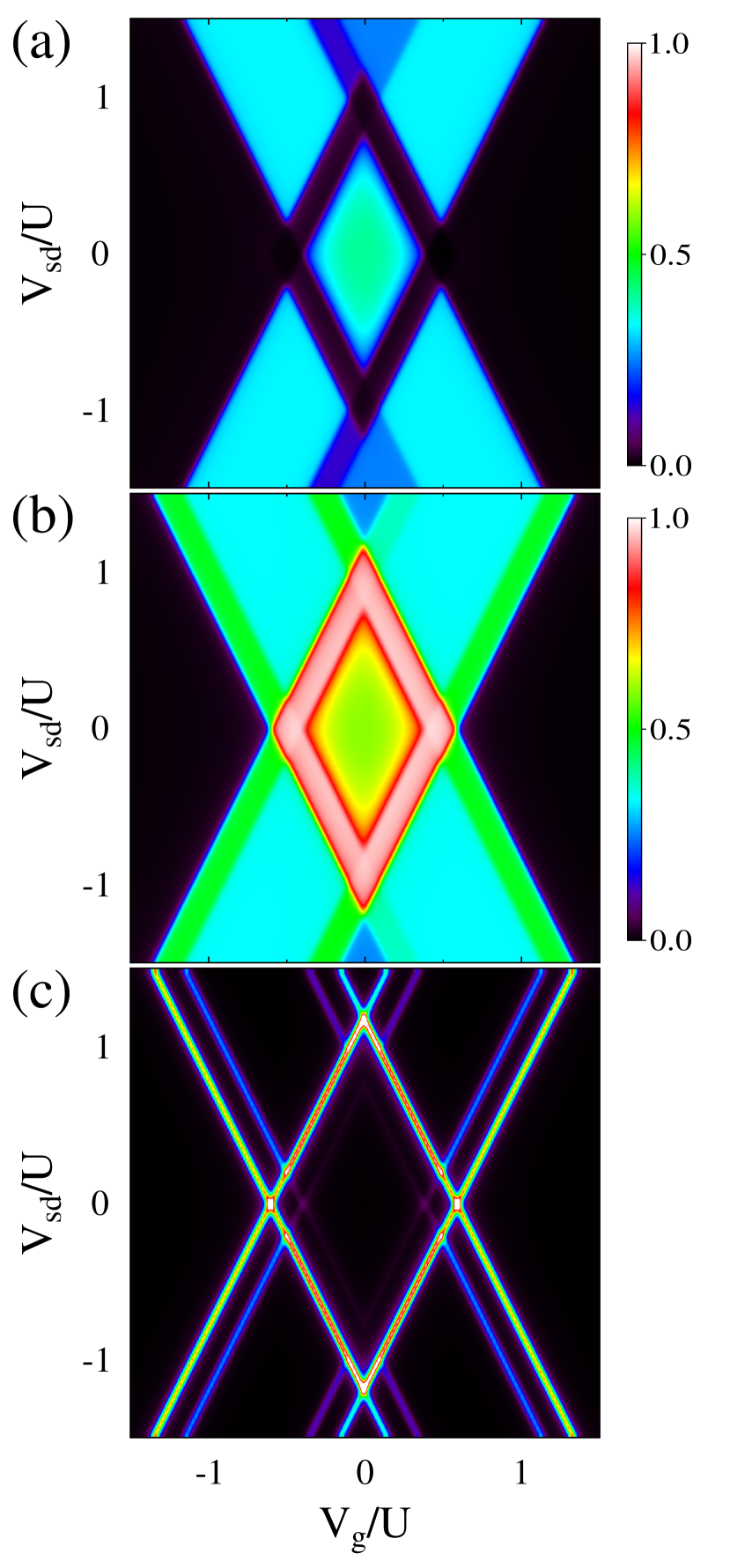
Figure 1: (Color online) QD in Coulomb blockade regime. Shown are maps of (a) probability of state $\lvert\uparrow\rangle$, $P_{\uparrow}$; (b) probability of state $\lvert\downarrow\rangle$, $P_{\downarrow}$; and (c) conductance, $dI/dV_{sd}$. See text for parameters.

III.2 Coulomb blockade in QD

Next we turn to a quantum dot in a junction with paramagnetic leads. The model Hamiltonian is

$$\hat{H}= \sum_{\sigma}\varepsilon_{\sigma}\hat{n}_{\sigma}+U\hat{n}_{\uparrow}\hat{n}_{\downarrow}+\sum_{k,\sigma}\varepsilon_{k}\hat{c}_{k\sigma}^{\dagger}\hat{c}_{k\sigma}$$ (24)

$$+ \sum_{k,\sigma}\left(V_{k}\hat{d}_{\sigma}^{\dagger}\hat{c}_{k\sigma}+H.c.\right)$$

where $\varepsilon_{\sigma}=\varepsilon-\sigma g\mu_{B}B_{dc}/2$ ($g$ is the Lande factor, $\mu_{B}$ is the Bohr magneton, $B_{dc}$ is the amplitude of dc magnetic field), $\hat{n}_{\sigma}=\hat{d}_{\sigma}^{\dagger}\hat{d}_{\sigma}$, and U is Coulomb repulsion term.

Elementary system excitations (as in Section III.1) are not the best choice for the initial vector operator. Such a starting point will lead to a Hartree-type treatment at the first step of the EOM chain. For strong $U$ a more suitable choice is a non-equilibrium atomic limit, where state resolved system excitations (Hubbard operators) form $\hat{a}_{1}$

$$\hat{a}_{1}\equiv\hat{A}_{1}=\left((1-\hat{n}_{\downarrow})\hat{d}_{\uparrow},\,(1-\hat{n}_{\uparrow})\hat{d}_{\downarrow},\,\hat{n}_{\downarrow}\hat{d}_{\uparrow},\,\hat{n}_{\uparrow}\hat{d}_{\downarrow}\right)^{T}$$ (25)

where $(\ldots)^{T}$ is transpose operation. Its spectral weight and free evolution matrices are

$$\mathbf{P}_{A_{1},A_{1}}=\mbox{diag}\left[1-\langle\hat{n}_{\downarrow}\rangle,\,1-\langle\hat{n}_{\uparrow}\rangle,\langle\hat{n}_{\downarrow}\rangle,\,\langle\hat{n}_{\uparrow}\rangle\right]$$ (26)

$$\mathbf{\varepsilon}_{1}=\mbox{diag}\left[\varepsilon_{\uparrow},\,\varepsilon_{\downarrow},\,\varepsilon_{\uparrow}+U,\,\varepsilon_{\downarrow}+U\right]$$ (27)

Here we want to restrict consideration to the Coulomb blockade regime, i.e. all the bath-assisted spin-spin correlations can be neglected (these correlations are important for the Kondo effect, as discussed below in Section III.3). This leads to

$$\hat{A}_{2}=\left((1-\hat{n}_{\downarrow})\hat{c}_{k\uparrow},\,(1-\hat{n}_{\uparrow})\hat{c}_{k\downarrow},\,\hat{n}_{\downarrow}\hat{c}_{k\uparrow},\,\hat{n}_{\uparrow}\hat{c}_{k\downarrow}\right)^{T}$$ (28)

$$\mathbf{P}_{A_{2},A_{2}}=\mbox{diag}\left[1-\langle\hat{n}_{\downarrow}\rangle,\,1-\langle\hat{n}_{\uparrow}\rangle,\langle\hat{n}_{\downarrow}\rangle,\,\langle\hat{n}_{\uparrow}\rangle\right]$$ (29)

$$\mathbf{\varepsilon}_{2}=\mbox{diag}\left[\varepsilon_{k},\,\varepsilon_{k},\,\varepsilon_{k}+U,\,\varepsilon_{k}+U\right]$$ (30)

and $\mathcal{W}_{1}\equiv\mathbf{\varepsilon}_{1}$.

Truncating the EOM chain (14) at the second step by neglecting self-energy $\mathcal{S}^{(1)}_{A_{2},A_{2}}$ we get a Dyson equation for canonical Green function $\mathcal{G}^{(0)}_{A_{1},A_{1}}(\tau,\tau^{\prime})$ with self-energy

$$\mathcal{S}^{(0)}_{A_{1},A_{1}}(\tau,\tau^{\prime})= \mbox{diag}\bigg{[}\Sigma_{\uparrow}(\tau,\tau^{\prime}),\,\Sigma_{\downarrow}(\tau,\tau^{\prime}),\,$$ (31)

$$\qquad\quad\Sigma_{\uparrow}(\tau,\tau^{\prime}),\,\Sigma_{\downarrow}(\tau,\tau^{\prime})\bigg{]}$$

where $\Sigma_{\sigma}(\tau,\tau^{\prime})\equiv\sum_{k}|V_{k}|^{2}g_{k\sigma}(\tau,\tau^{\prime})$, and $g_{k\sigma}(\tau,\tau^{\prime})\equiv-i\langle T_{c}\,\hat{c}_{k\sigma}(\tau)\,\hat{c}_{k\sigma}^{\dagger}(\tau^{\prime})\rangle$ is the Green function of free electrons in the contacts.

Utilizing relation $\hat{d}_{\sigma}=(1-\hat{n}_{\bar{\sigma}})\hat{d}_{\sigma}+\hat{n}_{\bar{\sigma}}\hat{d}_{\sigma}$ (here $\bar{\sigma}$ is spin projection opposite to $\sigma$), one can express the standard non-equilibrium Green function $G_{\sigma}(\tau,\tau^{\prime})\equiv-i\langle T_{c}\,\hat{d}_{\sigma}(\tau)\,\hat{d}_{\sigma}^{\dagger}(\tau^{\prime})\rangle$ as a combination of Hubbard non-equilibrium Green functions $\mathbf{G}^{(0)}_{A_{1},A_{1}}(\tau,\tau^{\prime})$. The resulting expression is

$$G_{\sigma}(\tau,\tau^{\prime})=\left[1-\langle\hat{n}_{\bar{\sigma}}\rangle\right]G(\tau,\tau^{\prime})+\langle\hat{n}_{\bar{\sigma}}\rangle G_{U}(\tau,\tau^{\prime})$$ (32)

where $G(\tau,\tau^{\prime})$ and $G_{U}(\tau,\tau^{\prime})$ are non-equilibrium Green functions defined by the following Dyson equations

$$\left[i\frac{\partial}{\partial\tau}-\varepsilon_{\sigma}\right]G(\tau,\tau^{\prime})=\delta(\tau,\tau^{\prime})$$ (33)

$$\qquad\qquad+\int_{c}d\tau_{1}\,\Sigma_{\sigma}(\tau,\tau_{1})\,G(\tau_{1},\tau^{\prime})$$

$$\left[i\frac{\partial}{\partial\tau}-\varepsilon_{\sigma}-U\right]G_{U}(\tau,\tau^{\prime})=\delta(\tau,\tau^{\prime})$$ (34)

$$\qquad\qquad+\int_{c}d\tau_{1}\,\Sigma_{\sigma}(\tau,\tau_{1})\,G_{U}(\tau_{1},\tau^{\prime})$$

We note that Eq.(32) coincides with Eq.(21) of Ref. Galperin et al., 2007b, where it was obtain from the standard EOM approach. However, while a special symmetrization procedure had to be implemented in the latter case (see Eq.(A23) of Ref. Galperin et al., 2007b) here the same expression is obtained in the symmetrized form automatically. This is an example of the built-in symmetrization property of the formulation, which otherwise should be obtained within a step-by-step approach.Levy and Rabani (2013a); Levy and Rabani (2013b) Note also that in the Coulomb blockade regime the EOM for the canonical Green function $\mathcal{G}^{(0)}_{A_{1},A_{1}}(\tau,\tau^{\prime})$ can be solved directly (without a self-consistent procedure). This is reminiscent of the similar observation in Ref. Galperin et al., 2007b (see discussion below Eq.(43) there).

The spectral weight $\mathbf{P}_{A_{1},A_{1}}$ is calculated from the lesser projections of the canonical Green function $\mathcal{G}^{(0)}_{A_{1},A_{1}}$ using

$$n_{\uparrow}= \frac{(1-I_{2})\,I_{1}+I_{2}\,I_{3}}{1-(I_{1}-I_{3})(I_{2}-I_{4})}$$ (35)

$$n_{\downarrow}= \frac{(1-I_{1})\,I_{2}+I_{1}\,I_{4}}{1-(I_{1}-I_{3})(I_{2}-I_{4})}$$ (36)

where $I_{m}\equiv-i\mathcal{G}^{(0)\,<}_{A_{1}^{(m)},A_{1}^{(m)}}(t,t)$ ($A_{1}^{(m)}$ indicates $m^{th}$ operator of the vector $\hat{A}_{1}$).

In addition to the level populations, probabilities of many-body states of the quantum dot, $\lvert 0\rangle$, $\lvert\sigma\rangle$, and $\lvert 2\rangle$, can be evaluated from

$$P_{\uparrow}=-i\mathbf{G}^{(0)\,<}_{A_{1}^{(1)},A_{1}^{(1)}}(t,t)\quad P_{\downarrow}=-i\mathbf{G}^{(0)\,<}_{A_{1}^{(2)},A_{1}^{(2)}}(t,t)$$ (37)

$$P_{2}=-i\mathbf{G}^{(0)\,<}_{A_{1}^{(3)},A_{1}^{(3)}}(t,t)=-i\mathbf{G}^{(0)\,<}_{A_{1}^{(4)},A_{1}^{(4)}}(t,t)$$

and $P_{0}=1-P_{\uparrow}-P_{\downarrow}-P_{2}$.

Figure 1 shows results of calculations which employ EOM for the canonical Green function $\mathcal{G}^{(0)}_{A_{1},A_{1}}(\tau,\tau^{\prime})$. Parameters are (in units of $U$): temperature $T=10^{-3}$, quantum dot levels $\varepsilon_{\uparrow}=-0.4$ and $\varepsilon_{\downarrow}=-0.6$, electronic escape rate to contact $K$ ($K=L,R$) $\Gamma_{K}\equiv 2\pi\sum_{k}|V_{k}|^{2}\delta(E-\varepsilon_{k})=0.01$ (we assume the wide band limit, where the escape rate does not depend on energy $E$). The Fermi energy is taken at origin $E_{F}=0$, and bias is applied symmetrically, $\mu_{L}=E_{F}+V_{sd}/2$ and $\mu_{R}=E_{F}-V_{sd}/2$. Gate potential shifts level positions $\varepsilon_{\sigma}\to\varepsilon_{\sigma}+V_{g}$. Calculations are performed on an energy grid spanning the region from $-3$ to $3$ with step $10^{-4}$. Probabilities of states $\lvert\uparrow\rangle$ and $\lvert\downarrow\rangle$ (see Figs. 1a and b) are seen to be equal in the blockaded and transition regions, but differ considerably at the borders of the two, where the probability of the state $\lvert\downarrow\rangle$ is much higher due to the lower position of its energy level. Fig. 1c shows a conductance map with spin sidebands. The result is in agreement with experimental observation.Park et al. (2002)

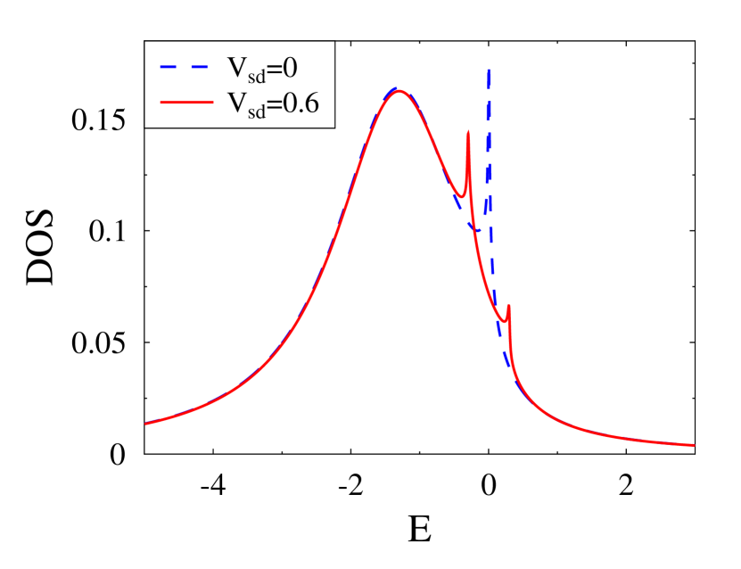
Figure 2: (Color online) Kondo in QD. Density of states, $-\mbox{Im}\,G^{r}_{\sigma}(E)/\pi$, in equilibrium (dashed line, blue) and biased $V_{sd}=0.6$ (solid line, red) junction. See text for parameters.

III.3 Kondo in QD

We continue consideration of the QD model, Eq.(24). Note that any nonequilibrium atomic limit (by its construction taking all interactions in the system into account exactly, but treating system-bath coupling perturbatively) is not a proper starting point to describe effects of the Kondo type, where entanglement between the system and bath has to be taken into account in a non-perturbative manner. Thus it is not reasonable to expect that the results presented below reproduce Kondo features exactly. So we compare our treatment to standard EOM approaches available in the literature.Galperin et al. (2007b); Meir et al. (1993); Zhang et al. (2003); Hattori (2008); Fransson and Zhu (2008)

To obtain Kondo features, one has to truncate the EOM chain at least on the third step.Galperin et al. (2007b); Meir et al. (1993) Correspondingly, in the present approach one has to work with three-dimensional energy grid. To avoid heavy computations we make the following simplifications: 1. Kondo is observed for $U\to\infty$, thus all Hubbard operators corresponding to double occupation of QD can be neglected; 2. The effect describes coherence between system and bath, thus excitations in both should be accounted for from the start; 3. Correlations responsible for appearance of a Kondo peak include bath-induced spin-spin correlations in the system, thus to simplify the consideration we include excitations of this type into the initial vector operator $\hat{a}_{1}$; 4. For simplicity we neglect system-induced spin-spin correlations in the bath.

With these approximations in mind an initial choice is

$$\hat{A}_{1}=\bigg{(}(1-\hat{n}_{\bar{\sigma}})\hat{d}_{\sigma},\,(1-\hat{n}_{\bar{\sigma}})\hat{c}_{k\sigma},\,\hat{d}_{\bar{\sigma}}^{\dagger}\hat{c}_{k\bar{\sigma}}\hat{d}_{\sigma}\bigg{)}^{T}$$ (38)

where $\sigma=\uparrow,\downarrow$, $\hat{n}_{\sigma}\equiv\hat{d}_{\sigma}^{\dagger}\hat{d}_{\sigma}$, and $\hat{n}_{k\sigma}\equiv\hat{c}_{k\sigma}^{\dagger}\hat{c}_{k\sigma}$. Corresponding spectral weight and free evolution matrices have block spin structure

$$\mathbf{P}_{A_{1},A_{1}}^{(\sigma)}=$$ (39)

$$\begin{bmatrix}\langle 1-\hat{n}_{\bar{\sigma}}\rangle&0&\langle(1-\hat{n}_{\sigma})\hat{c}_{k\bar{\sigma}}^{\dagger}\hat{d}_{\bar{\sigma}}\rangle\\ 0&\langle 1-\hat{n}_{\bar{\sigma}}\rangle&\langle\hat{c}_{k\bar{\sigma}}^{\dagger}\hat{c}_{k\sigma}\,\hat{d}_{\sigma}^{\dagger}\hat{d}_{\bar{\sigma}}\rangle\\ \langle(1-\hat{n}_{\sigma})\hat{d}^{\dagger}_{\bar{\sigma}}\hat{c}_{k\bar{\sigma}}\rangle&\langle\hat{c}_{k\sigma}^{\dagger}\hat{c}_{k\bar{\sigma}}\,\hat{d}_{\bar{\sigma}}^{\dagger}\hat{d}_{\sigma}\rangle&\langle\hat{n}_{\bar{\sigma}}+(\hat{n}_{\sigma}-\hat{n}_{\bar{\sigma}})\hat{n}_{k\bar{\sigma}}\rangle\end{bmatrix}$$

$$\mathbf{\varepsilon}_{1}^{(\sigma)}=\begin{bmatrix}\varepsilon_{\sigma}&V_{k\sigma}&-V_{k\bar{\sigma}}\\ \overset{*}{V}_{k\sigma}&\varepsilon_{k\sigma}&0\\ 0&0&\varepsilon_{k\bar{\sigma}}-\varepsilon_{\bar{\sigma}}+\varepsilon_{\sigma}\end{bmatrix}$$ (40)

Neglecting system-induced spin correlations in the bath we get

$$\hat{a}_{2}=\bigg{(}\hat{n}_{k\bar{\sigma}}\hat{d}_{\sigma}\bigg{)}^{T}$$ (41)

$$\mathbf{P}_{a_{2},A_{1}}^{(\sigma)}=\begin{bmatrix}\langle(1-\hat{n}_{\bar{\sigma}})\hat{n}_{k\bar{\sigma}}\rangle&0&\langle(1-\hat{n}_{\sigma})\hat{c}^{\dagger}_{k\bar{\sigma}}\hat{d}_{\bar{\sigma}}\rangle\end{bmatrix}$$ (42)

To allow for analytic derivation we make an additional approximation, decoupling system and bath degrees of freedom in $\mathbf{P}_{A_{1},A_{1}}$ and $\mathbf{P}_{a_{2},A_{1}}$. Note that this type of approximations should be done with care. In particular, derivation of the symmetrized version for free evolution presented in Section II.2 is not possible after the approximation, and free evolution term in Eq. (14), should be taken in the form presented in Eq.(85). Fortunately, in this particular case the resulting EOM for the system part of the canonical Green function (canonical correlation function of the first operator in the vector $\hat{A}_{1}$, Eq(38)) is the same if derived from left or right EOM. Explicit expression for the EOM is

$$\left(i\frac{\partial}{\partial\tau}-\varepsilon_{\sigma}\right)\mathcal{G}^{(0)}_{A_{1}^{(1)},A_{1}^{(1)}}(\tau,\tau^{\prime})=\delta(\tau,\tau^{\prime})$$ (43)

$$+\int_{c}d\tau_{1}\left(\Sigma_{\sigma}(\tau,\tau_{1})+\Sigma_{\sigma}^{(K)}(\tau,\tau_{1})\right)\mathcal{G}^{(0)}_{A_{1}^{(1)},A_{1}^{(1)}}(\tau_{1},\tau^{\prime})$$

where self-energy $\Sigma_{\sigma}(\tau,\tau^{\prime})$ is defined below Eq.(31) and

$$\Sigma_{\sigma}^{(K)}(\tau,\tau^{\prime})\equiv\sum_{k}\lvert V_{k}\rvert^{2}\langle\hat{n}_{k\bar{\sigma}}\rangle g_{k\bar{\sigma}}^{(K)}(\tau,\tau^{\prime})$$ (44)

with

$$\left(i\frac{\partial}{\partial\tau}-\varepsilon_{k\bar{\sigma}}+\varepsilon_{\bar{\sigma}}-\varepsilon_{\sigma}\right)g_{k\bar{\sigma}}^{(K)}(\tau,\tau^{\prime})=\delta(\tau,\tau^{\prime})$$ (45)

defining the contact electron Green function. The latter self-energy is responsible for appearance of Kondo features. We note that the corresponding standard non-equilibrium Green function, $G_{\sigma}(\tau,\tau^{\prime})\equiv(1-\langle\hat{n}_{\bar{\sigma}}\rangle)\mathcal{G}^{(0)}_{A_{1}^{(1)},A_{1}^{(1)}}(\tau,\tau^{\prime})$ coincides with the result obtained in our previous publication (see Eq.(53) in Ref. Galperin et al., 2007b). Note also that element $\langle\hat{n}_{k\bar{\sigma}}\rangle$ in Eq.(44), central for appearance of Kondo features, is obtained as a result of projection (orthogonalization), Eqs. (4) and (5).

Figure 2 shows results of calculations that employ EOM for the canonical Green function $\mathcal{G}^{(0)}_{A_{1}^{(1)},A_{1}^{(1)}}(\tau,\tau^{\prime})$, Eq.(43). Parameters are (in units of $\Gamma$): $T=0.005$, $\varepsilon_{\sigma}=-2$, and $\Gamma_{L}=\Gamma_{R}=0.5$. Fermi energy is taken at origin, $E_{F}=0$, and bias is applied symmetrically, $\mu_{L}=E_{F}+V_{sd}/2$ and $\mu_{R}=E_{F}-V_{sd}/2$. Calculations are performed on an energy grid spanning the region from $-5$ to $3$ with step $10^{-4}$. The density of states (same for both spins) in equilibrium demonstrates a Kondo feature at $E_{F}$. Under bias the feature splits into two peaks centered around each of the chemical potentials. This result was first reported in Ref. Meir et al., 1993.

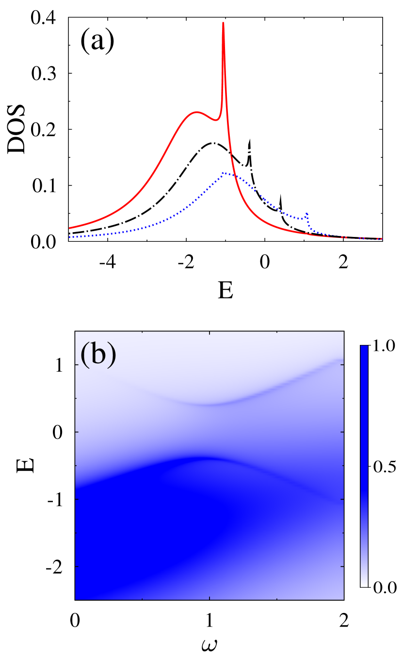
Figure 3: (Color online) Kondo in QD in the presence of ac magnetic field with frequency $\omega$. (a) Density of states, $\rho_{\sigma}(E,\omega)\equiv-\mbox{Im}\left[\mathbf{U}\,\mathbf{G}^{(0)\,r}_{A_{1}^{(1)},A_{1}^{(1)}}(E)\,\mathbf{U}^{\dagger}\right]_{\sigma\sigma}/\pi$ for $\omega=0,\sigma=\uparrow$ (solid line, red), $\omega=0,\sigma=\downarrow$ (dotted line, blue), and $\omega=1$ (dash-dotted line, black). (b) Map of $\rho_{\uparrow}(E,\omega)$. See text for parameters.

In the presence of an ac magnetic field Hamiltonian (24) acquires an additional time-dependent term

$$-g\mu_{B}B_{ac}\left(\hat{d}^{\dagger}_{\uparrow}\hat{d}_{\downarrow}e^{i\omega t}+\hat{d}_{\downarrow}\hat{d}_{\uparrow}e^{-i\omega t}\right)$$ (46)

Here $B_{ac}$ is the amplitude and $\omega$ is the frequency of the ac magnetic field. Transformation to the rotational frame of the field

$$\hat{\bar{H}}=i\left(\frac{\partial}{\partial t}e^{\hat{S}(t)}\right)e^{-\hat{S}(t)}+e^{\hat{S}(t)}\hat{H}e^{-\hat{S}(t)}$$ (47)

$$\hat{S}(t)=-\frac{i}{2}\omega t\sum_{\sigma}\sigma\left(\hat{n}_{\sigma}+\sum_{k}\hat{n}_{k\sigma}\right)$$

allows us to formulate an effective time-independent problem. Finally, transformation into molecular eigenbasis leads to

$$\hat{H}_{eig}=\sum_{\sigma}E_{\sigma}\hat{c}_{\sigma}^{\dagger}\hat{c}_{\sigma}+U\hat{n}^{c}_{\uparrow}\hat{n}^{c}_{\downarrow}+\sum_{k\sigma}\bar{\varepsilon}_{k\sigma}\hat{c}^{\dagger}_{k\sigma}\hat{c}_{k\sigma}$$ (48)

$$+\sum_{k}\left[\left(\hat{c}_{\uparrow}^{\dagger},\hat{c}^{\dagger}_{\downarrow}\right)\mathbf{U}^{\dagger}V_{k}\binom{\hat{c}_{k\uparrow}}{\hat{c}_{k\downarrow}}+\left(\hat{c}_{k\uparrow}^{\dagger},\hat{c}_{k\downarrow}^{\dagger}\right)V_{k}^{*}\mathbf{U}\binom{\hat{c}_{\uparrow}}{\hat{c}_{\downarrow}}\right]$$

where $\hat{n}^{c}_{\sigma}=\hat{c}_{\sigma}^{\dagger}\hat{c}_{\sigma}$, $\bar{\varepsilon}_{k\sigma}=\varepsilon_{k}+\sigma\omega/2$, and

$$\mathbf{U}=\begin{bmatrix}\cos\theta&-\sin\theta\\ \sin\theta&\cos\theta\end{bmatrix};\qquad\tan 2\theta=\frac{2\lvert g\mu_{B}B_{ac}\rvert}{\omega-g\mu_{B}B_{dc}}$$ (49)

$$E_{\sigma}=\varepsilon+\frac{\sigma}{2}\sqrt{(\omega-g\mu_{B}B_{dc})^{2}+4(g\mu_{B}B_{ac})^{2}}$$ (50)

Treatment within the projection operator NEGF EOM (PO-NEGF EOM) approach is similar to the one discussed above. Initial vector operator is

$$\hat{A}_{1}= \bigg{(}(1-\hat{n}^{c}_{\bar{\sigma}})\hat{c}_{\sigma},\,(1-\hat{n}^{c}_{\bar{\sigma}})\hat{c}_{k\sigma},\,\hat{c}_{\bar{\sigma}}^{\dagger}\hat{c}_{k\bar{\sigma}}\hat{c}_{\sigma},$$ (51)

$$(1-\hat{n}^{c}_{\sigma})\hat{c}_{k\sigma},\,\hat{c}_{\bar{\sigma}}^{\dagger}\hat{c}_{k\sigma}\hat{c}_{\sigma}\bigg{)}^{T}$$

which yields in the second step

$$\hat{a}_{2}=\bigg{(}\hat{n}_{k\bar{\sigma}}\hat{c}_{\sigma},\,\hat{n}_{k\sigma}\hat{c}_{\sigma}\bigg{)}^{T}$$ (52)

The set of approximations outlined above Eq.(38) eventually leads to

$$\left(i\frac{\partial}{\partial\tau}\mathbf{I}-\mathbf{E}\right)\mathbf{G}^{(0)}_{A_{1}^{(1)},A_{1}^{(1)}}(\tau,\tau^{\prime})=\delta(\tau,\tau^{\prime})\mathbf{P}$$ (53)

$$+\int_{c}d\tau_{1}\left(\mathbf{\Sigma}^{(K0)}(\tau,\tau_{1})+\mathbf{\Sigma}^{(K1)}(\tau,\tau_{1})+\mathbf{\Sigma}^{(K2)}(\tau,\tau_{1})\right)$$

$$\qquad\qquad\times\mathbf{G}^{(0)}_{A_{1}^{(1)},A_{1}^{(1)}}(\tau_{1},\tau^{\prime})$$

where free evolution, Green function and self-energies are $2\times 2$ matrices in the spin space, $\mathbf{I}$ is the unit matrix, $\mathbf{E}=\mbox{diag}[E_{\uparrow},E_{\downarrow}]$, and $\mathbf{\Sigma}^{(K0)}(\tau,\tau^{\prime})=\mathbf{U}^{\dagger}\mathbf{\Sigma}(\tau,\tau^{\prime})\mathbf{U}$. $\mathbf{\Sigma}(\tau,\tau^{\prime})$, $\mathbf{\Sigma}^{(K1)}(\tau,\tau^{\prime})$, and $\mathbf{\Sigma}^{(K2)}(\tau,\tau^{\prime})$ are the diagonal in spin space matrices defined as

$$\Sigma_{\sigma}(\tau,\tau^{\prime})\equiv \sum_{k}\lvert V_{k}\rvert^{2}\bar{g}_{k\sigma}(\tau,\tau^{\prime})$$ (54)

$$\Sigma_{\sigma}^{(K1)}(\tau,\tau^{\prime})\equiv \cos^{2}\theta\sum_{k}\lvert V_{k}\rvert^{2}\langle\hat{n}_{k\bar{\sigma}}\rangle\bar{g}^{(1)}_{k\bar{\sigma}}(\tau,\tau^{\prime})$$ (55)

$$\Sigma_{\sigma}^{(K2)}(\tau,\tau^{\prime})\equiv \sin^{2}\theta\sum_{k}\lvert V_{k}\rvert^{2}\langle\hat{n}_{k\sigma}\rangle\bar{g}^{(2)}_{k\sigma}(\tau,\tau^{\prime})$$ (56)

with

$$\left(i\frac{\partial}{\partial\tau}-\bar{\varepsilon}_{k\sigma}\right)\bar{g}_{k\sigma}(\tau,\tau^{\prime})=\delta(\tau,\tau^{\prime})$$ (57)

$$\left(i\frac{\partial}{\partial\tau}-\bar{\varepsilon}_{k\sigma}+\varepsilon_{\sigma}-\varepsilon_{\bar{\sigma}}\right)\bar{g}_{k\sigma}^{(1)}(\tau,\tau^{\prime})=\delta(\tau,\tau^{\prime})$$ (58)

$$\left(i\frac{\partial}{\partial\tau}-\bar{\varepsilon}_{k\sigma}+\varepsilon_{\bar{\sigma}}-\varepsilon_{\sigma}\right)\bar{g}_{k\sigma}^{(2)}(\tau,\tau^{\prime})=\delta(\tau,\tau^{\prime})$$ (59)

$\mathbf{P}$ is spectral weight

$$\mathbf{P}=\begin{bmatrix}\langle 1-\hat{n}^{c}_{\downarrow}\rangle&\langle\hat{c}_{\downarrow}^{\dagger}\hat{c}_{\uparrow}\rangle\\ \langle\hat{c}_{\uparrow}^{\dagger}\hat{c}_{\downarrow}\rangle&\langle 1-\hat{n}^{c}_{\uparrow}\rangle\end{bmatrix}$$ (60)

Neglecting the off-diagonal elements in the spectral weight $\mathbf{P}$ we recover the approximation discussed in Refs. Zhang et al., 2003; Hattori, 2008; Fransson and Zhu, 2008. Note that similar to consideration in Section III.1 and contrary to discussion in Ref. Zhang et al., 2003 no self-consistent calculation is necessary within the approximation.

Figure 3 shows density of states, $\rho_{\sigma}(E,\omega)\equiv-\mbox{Im}\left[\mathbf{U}\,\mathbf{G}^{(0)\,r}_{A_{1}^{(1)},A_{1}^{(1)}}(E)\,\mathbf{U}^{\dagger}\right]_{\sigma\sigma}/\pi$, for the Kondo feature in the presence of an ac magnetic field. Parameters of the calculation are (in units of $\Gamma$): $\varepsilon_{\uparrow}=-2.5$, $\varepsilon_{\downarrow}=-1.5$, $g\mu_{B}B_{ac}=0.2$, and $V_{sd}=0$. Other parameters are as in Fig. 2. In this case densities for spin up and down are in general different (see solid and dotted lines in Fig. 3a). They coincide at $\omega=1$ (dash-dotted line in Fig. 3a), where the frequency of the field is in resonance with molecular excitation, $\omega=\lvert\varepsilon_{\uparrow}-\varepsilon_{\downarrow}\rvert$. Fig. 3b illustrates an avoided crossing demonstrated by Kondo peaks of the two densities when the frequency of the ac magnetic field approaches molecular resonance.

III.4 Two-level system

As a last example we consider a particular case of Hamiltonian (21) with $M=2$. However instead of using quasiparticle excitation operators, $\hat{d}_{m}$, we perform the analysis employing (in the spirit of the non-equilibrium atomic limit) Hubbard operators. The initial vector-operator is

$$\hat{A}_{1}=\bigg{(}\hat{X}_{0a},\hat{X}_{0b},\hat{X}_{b2},\hat{X}_{a2}\bigg{)}^{T}$$ (61)

where $\hat{X}_{S_{1}S_{2}}\equiv\lvert S_{1}\rangle\,\langle S_{2}\rvert$ are projection (Hubbard) operators, and $\lvert 0\rangle$, $\lvert a\rangle$, $\lvert b\rangle$, $\lvert 2\rangle$ are many-body states in the eigen-basis of molecular Hamiltonian $\mathbf{H}^{(M)}$. The choice (61) leads to

$$\mathbf{P}_{A_{1},A_{1}}=$$ (62)

$$\begin{bmatrix}\langle\hat{X}_{00}+\hat{X}_{aa}\rangle&\langle\hat{X}_{ba}\rangle&0&0\\ \langle\hat{X}_{ab}\rangle&\langle\hat{X}_{00}+\hat{X}_{bb}\rangle&0&0\\ 0&0&\langle\hat{X}_{bb}+\hat{X}_{22}\rangle&\langle\hat{X}_{ba}\rangle\\ 0&0&\langle\hat{X}_{ab}\rangle&\langle\hat{X}_{aa}+\hat{X}_{22}\rangle\end{bmatrix}$$

$$\mathbf{\varepsilon}_{1}=\mbox{diag}\bigg{[}E_{a},E_{b},E_{a},E_{b}\bigg{]}$$ (63)

We note that the First Hubbard Approximation (HIA) partly misses renormalization of the free evolution matrix $\mathbf{\omega}_{1}$, Eq.(II.1), and completely neglects the self-energy $\mathbf{\Sigma}^{(0)}_{A_{1},A_{1}}$, Eq.(II.1).

As discussed in Section II.3, direct application of the methodology to transport problems in general is prohibitively expensive due to necessity to work with multi-energy correlation functions. Here we implement an approximation, where canonical self-energy is provided by solving self-consistently Eq.(II.3), and decoupling between system and bath variables is assumed in the correlation function $\mathcal{S}(\tau,\tau^{\prime})$.

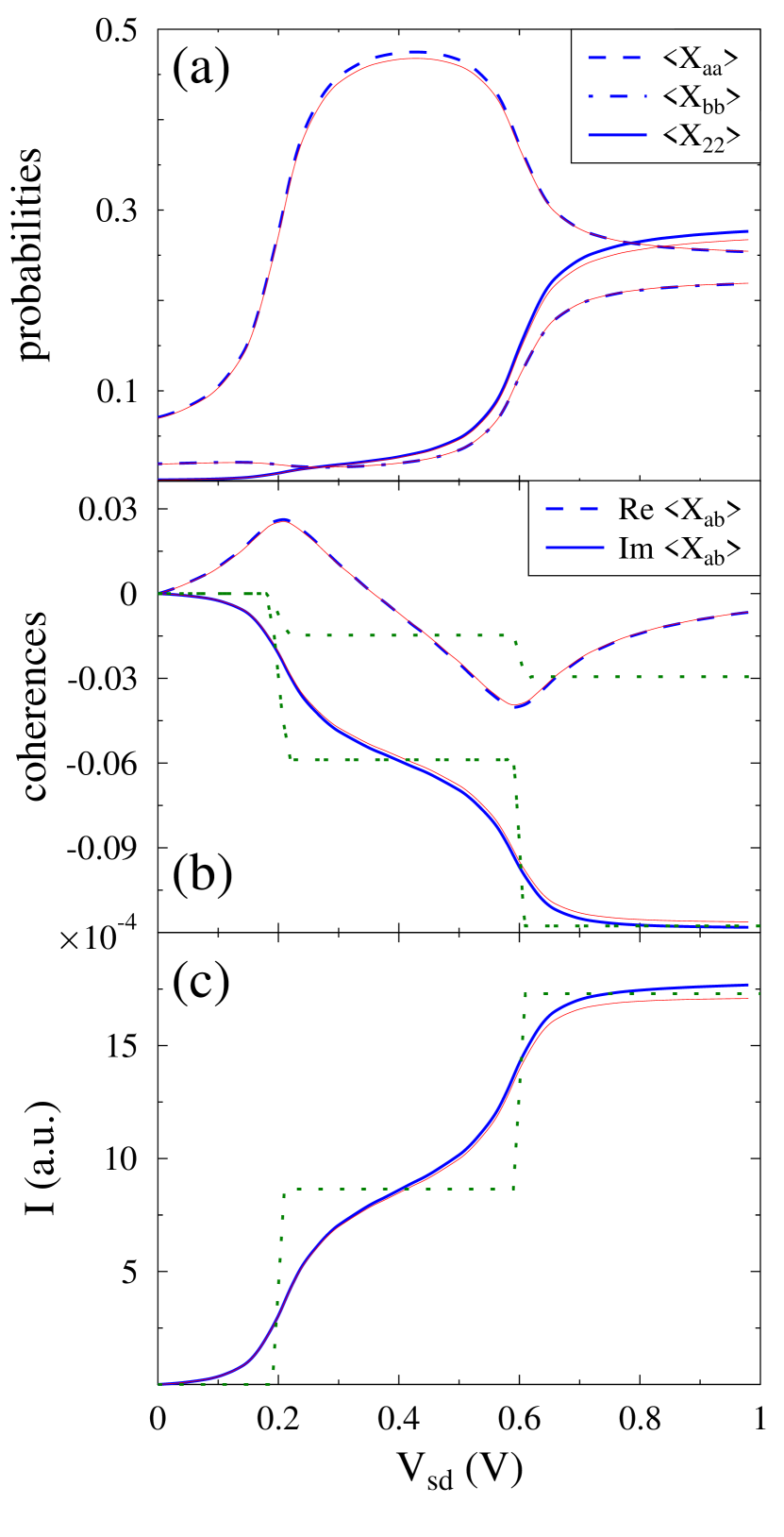
Figure 4: (Color online) Two-level system (TLS). Simulations are performed within the NEGF (solid line; red) and projection operator scheme of Section II.3 (solid, dashed, and dash-dotted lines; blue). Shown are (a) probabilities and (b) coherences of the many-body eigenstates of the TLS, and (c) current vs. applied bias $V_{sd}$. Panels (b) and (c) show also results of the Redfield QME simulation (dotted and double-dotted lines, green). See text for parameters.

This separation leads to the appearance of the canonical system Green functions $\mathcal{G}^{(0)}_{B_{1},B_{1}}(\tau,\tau^{\prime})$ generated by vector-operator

$$\hat{B}_{1}=\bigg{(}\hat{X}_{00},\hat{X}_{aa},\hat{X}_{bb},\hat{X}_{22},\hat{X}_{ab},\hat{X}_{ba},\hat{X}_{02}\bigg{)}^{T}$$ (64)

Writing EOMs for these Green functions is not straightforward, since $\mathbf{P}^{-1}_{B_{1},B_{1}}$ does not exist. Indeed, not every choice of operators yields a matrix which has an inverse. For example, commuting operators will provide a matrix without inverse. Two ways to proceed were suggested in Refs. Tserkovnikov, 1981, 1999, 1982: 1. Complementing the original vector operator with time derivatives of the commuting operators (this approach will resolve the issue, and corresponding formulation will be exact; however one has to work with big matrices); and 2. Formulations of an approximate practical scheme. To proceed we formulate such a scheme, where instead of single EOM for $\mathbf{G}^{(0)}_{B_{1},B_{1}}(\tau,\tau^{\prime})$, Eq.(74), two equations ($s=\pm$) are considered

$$i\frac{\partial}{\partial\tau}\mathbf{G}^{(s,0)}_{B_{1},B_{1}}(\tau,\tau^{\prime})=\delta(\tau,\tau^{\prime})\,\mathbf{P}^{(s)}_{B_{1},B_{1}}(\tau)+\mathbf{G}^{(s,0)}_{\dot{B_{1}},B_{1}}(\tau,\tau^{\prime}),$$ (65)

such that $\left[\mathbf{P}^{(s)}_{B_{1},B_{1}}\right]^{-1}$ exists, $\mathbf{P}_{B_{1},B_{1}}=\sum_{s=\pm}\mathbf{P}^{(s)}_{B_{1},B_{1}}$, and $\mathbf{G}^{(0)}_{a,b}(\tau,\tau^{\prime})=\sum_{s=\pm}\mathbf{G}^{(s,0)}_{a,b}(\tau,\tau^{\prime})$. Eqs. (65) can be solved according to the standard procedure described above, however each chain has its own definition of the orthogonalized operators, $\hat{A}_{2}^{(s)}\equiv\hat{a}_{2}-\mathbf{P}_{a_{2}A_{1}}\left[\mathbf{P}_{A_{1},A_{1}}^{(s)}\right]^{-1}\hat{A}_{1}$.

In particular, in the simulations below we chose $\mathbf{P}^{(s)}_{B_{1},B_{1}}(\tau)=\mathbf{P}_{B_{1},B_{1}}\pm\epsilon\mathbf{I}$ where $\epsilon$ is a small number and $\mathbf{I}$ is the unit matrix, and follow the formulation of Section II.3. In definitions of correlation functions $\mathcal{S}^{(s)}(\tau,\tau^{\prime})$ (see Eqs. (19) and (D)) for small $\epsilon$ we take approximately $\mathbf{G}^{(s,0)}_{a_{2},a_{2}}(\tau,\tau^{\prime})\approx\mathbf{G}_{a_{2},a_{2}}(\tau,\tau^{\prime})/2$. Decoupling system and bath variables in correlation functions $\mathcal{S}^{(s)}(\tau,\tau^{\prime})$ this time yields Green functions $\mathcal{G}^{(0)}_{A_{1},A_{1}}(\tau,\tau^{\prime})$, so that the two sets of equations have to be solved self-consistently.

Figure 4 shows results of calculations which employ the approximate approach of Section II.3 and compares it to exact results provided by standard NEGF. Parameters of the calculation are $T=10$ K, $H^{(M)}_{11}=H^{(M)}_{22}=0.4$ eV, $H^{(M)}_{12}\equiv t_{12}=0.2$ eV, $\Gamma^{L}_{11}=\Gamma^{R}_{22}=0.1$ eV and $\Gamma^{K}_{12}=\Gamma^{K}_{21}=0$ (here $K=L,R$ and $\Gamma^{K}_{m_{1}m_{2}}\equiv 2\pi\sum_{k\in K}V_{m_{1}k}V_{km_{2}}\delta(E-\varepsilon_{k})$). Fermi energy is chosen as the origin, $E_{F}=0$, and bias $V_{sd}$ is applied on the left, $\mu_{L}=E_{F}+V_{sd}$ and $\mu_{R}=E_{F}$. Calculation is performed on an energy grid spanning the region from $-3$ to $5$ eV with step $10^{-4}$ eV. Tolerance for convergence in populations and coherences is $10^{-4}$. One sees that probabilities of the many-body eigenstates of the system ($P_{0}=\langle\hat{X}_{00}\rangle$, $P_{a}=\langle\hat{X}_{aa}\rangle$, $P_{b}=\langle\hat{X}_{bb}\rangle$, $P_{2}=\langle\hat{X}_{22}\rangle$), coherences ($\langle X_{ab}\rangle$), and current-voltage characteristics of the junctions are accurately reproduced by the approximate procedure of Section II.3. Note that standard Redfield QME procedure, as an approach treating system-bath coupling to finite (second) order, misses broadening induced by hybridization.

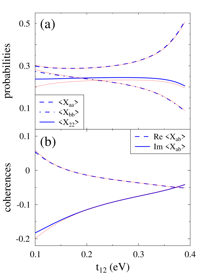
Figure 5: (Color online) Two-level system (TLS). Simulations are performed within the NEGF (solid line; red) and projection operator scheme of Section II.3 (solid, dashed, and dash-dotted lines; blue). Shown are (a) probabilities and (b) coherences of the many-body eigenstates of the TLS vs. electron hopping parameter $t_{12}$ at bias $V_{sd}=0.8$ V. Other parameters are as in Fig. 4.

Figure 5 shows probabilities and coherences of the many-body states as functions of the inter-level electron hopping parameter $t_{12}\equiv H^{(M)}_{12}$. Calculation is performed at $V_{sd}=0.8$ V, other parameters are as in Fig. 4. One sees that the approximate scheme of Section II.3 reproduces exact results pretty well while the description in terms of non-equilibrium atomic limit is meaningful, i.e. $t>\Gamma$.

IV Conclusions

Progress in experimental techniques at the nanoscale lead to the appearance of new branches of research. In particular, molecular optoelectronics, nanoplasmonics, and spintronics are examples of recent developments in the field of molecular electronics. These developments provide a challenge for proper theoretical description of measurements in strongly interacting open systems far from equilibrium. In particular, development of theoretical methods capable of simulating transport in molecular junctions in the language of the many-body states of an isolated system - the nonequilibrium atomic limit - is necessary for adequate description in such experimentally observed situations as breakdown of Born-Oppenheimer approximation, strong electron-vibration interaction (polaron formation), avoided crossing (polariton formation) due to strong molecule-plasmon interaction, and excitations in single molecule magnetic junctions.

A straightforward general methodology applicable in such situation is provided by the equation-of-motion technique. EOM formulated on the Keldysh contour has been used in the literature to describe transport in junctions by usGalperin et al. (2006); Galperin et al. (2007b) and others.Bulka and Kostyrko (2004); Kostyrko and Bułka (2005); Levy and Rabani (2013a); Levy and Rabani (2013b) Two main weaknesses of the method are: 1. The necessity to make uncontrollable approximations in truncating the (in general infinite) chain of EOMs and 2. Loss of symmetry properties (proper commutation relations) as a result of decoupling.

Here we introduce a non-equilibrium version of the EOM approach which is formulated with the help of projection operators (similar to quantum master equation formulations), and choice of irreducible Green functions in the EOM chain (similar to the choice of irreducible diagrams in the standard quantum field theory methods). The approach, originally developed by TserkovnikovTserkovnikov (1981, 1999) for description of systems at equilibrium, is reformulated to be applicable to (in general) time-dependent non-equilibrium situations (Section II.1). We derive an explicit canonical form for the chain of EOMs (see Section II.2), thus resolving concernsPedersen et al. (2009) related to a way of proper construction for a non-equilibrium atomic limit. After a general formulation we discuss application of the procedure to transport in junctions. A simple practical approach is proposed in Section II.3.

This PO-NEGF EOM (PO meaning Projection Operator) formulation is illustrated within simple model calculations. In particular, we consider models of multi-level non-interacting system, quantum dots in the Coulomb blockade and Kondo regimes, and a two-level system treated with Hubbard operators. The latter was the focus of Ref. Pedersen et al., 2009, when concerns about formulations of a non-equilibrium atomic limit were raised. Results of numerical simulations are compared to other approximate techniques, and (when available) to exact results. We show that proper symmetrization, as discussed in Refs. Bonch-Bruevich and Tyablikov, 1962; Levy and Rabani, 2013a; Levy and Rabani, 2013b, is built into the scheme. We also show explicitly that projection (orthogonalization) is crucial for proper description of a system coupled to the bath. The latter is missed within the first Hubbard approximation, as discussed in Refs. Galperin et al., 2008b; Pedersen et al., 2009 in connection with the Hubbard non-equilibrium Green function formulation, and may be the reason for inconsistencies within the approximation.

In summary, the presented approach is a step forward in development of NEGF-EOM approaches. While the proposed truncation procedure (similar to the standard EOM methods) cannot formally guarantee that the resulting approximation will be conserving in the sense of being derived from a Luttinger-Ward functional, it introduces two important features: 1. Controllability of the decoupling scheme and 2. Canonical form of the resulting EOM chain. The former is due to orthogonalization, Eqs. (4), (5), and (7), and is discussed in detail in Ref. Tserkovnikov, 1999. The latter, Eq.(14), is a new result, which guarantees Hermiticity and positive definiteness of the resulting density matrix. Moreover, it can be viewed as a way to introduce quasiparticles in the case of strong interactions localized on the molecule. Note that the quasiparticles are not molecular (or Kohn-Sham) orbitals of the isolated molecule. Application of the approach to problems, where standard NEGF methodology is not feasible, is the goal of future research.

Appendix A Positivity of spectral weights for Fermi-type excitation at finite temperature

Here we prove that for vector operators $A_{n}(\tau)=(\hat{X}_{1}(\tau),\ldots,\hat{X}_{M}(\tau))^{T}$ ($\{\hat{X}_{i}(\tau)\}$ are Hubbard operators of Fermi type) the spectral weight $\mathbf{P}_{A_{n},A_{n}}(\tau)$, Eq.(3, is a positive definite matrix at finite temperatures. The proof follows from observation that the spectral weight is the sum of two Gram matrices, the positive definite character of physical density matrix at finite temperature, and properties of the trace.

Let $A=(\hat{X}_{1},\dots,\hat{X}_{M})$ be a vector operator such that $\hat{X}_{i}$ is an operator of Fermi type for every $i$, then

$$\mathbf{P}_{A,A}=\mathbf{M}_{1}+\mathbf{M}_{2}$$ (66)

where

$$\mathbf{M}_{1}=\begin{bmatrix}\langle\hat{X}_{1}\hat{X}_{1}^{\dagger}\rangle&\ldots&\langle\hat{X}_{1}\hat{X}_{M}^{\dagger}\rangle\\ \vdots&\ddots&\vdots\\ \langle\hat{X}_{M}\hat{X}_{1}^{\dagger}\rangle&\ldots&\langle\hat{X}_{n}\hat{X}_{M}^{\dagger}\rangle\\ \end{bmatrix},$$ (67)

with $\langle\hat{X}_{i}\hat{X}_{j}^{\dagger}\rangle=\rm{Tr}\{\hat{\rho}\,\hat{X}_{i}\,\hat{X}_{j}^{\dagger}\}$. Similarly, matrix $\mathbf{M}_{2}$ is composed by $\langle\hat{X}_{j}^{\dagger}\hat{X}_{i}\rangle$ elements.

For any nonzero $M$-dimensional complex column vector ${\rm y}=(y_{1},\dots,y_{M})^{T}$ we can write

$${\rm y}^{\dagger}\cdot\mathbf{M}_{1}\cdot{\rm y}=\sum_{i,j}^{M}y_{i}^{*}\langle\hat{X}_{i}\hat{X}_{j}^{\dagger}\rangle y_{j}\equiv\left\langle\hat{C}\,\hat{C}^{\dagger}\right\rangle$$ (68)

where $\hat{C}\equiv\sum_{i}^{M}y_{i}^{*}\hat{X}_{i}$ and we have used that trace is a linear function.

Since the operators $\hat{X}_{i}$ are linearly independent, $\hat{C}$ is not the zero matrix in any basis for any non-trivial choice of $\rm y$. Let $\rm{c}_{i}$ be the $i$-th column vector in $\mathbf{C}$. By invariance of the trace under cyclic permutations we get

$$\left\langle\hat{C}\,\hat{C}^{\dagger}\right\rangle=\rm{Tr}\{\hat{C}^{\dagger}\rho\hat{C}\}=\sum_{i}\rm{c}_{i}^{\dagger}\cdot\mathbf{\rho}\cdot\rm{c}_{i}$$ (69)

Sum on the right is strictly positive as at least one vector $\rm{c}_{i}$ is nonzero and the density matrix $\mathbf{\rho}$ is positive definite. This proves that matrix $\mathbf{M}_{1}$ is positive definite.

Similarly we can find that $\mathbf{M}_{2}$ is also positive definite matrix. Thus, for any non-zero complex vector $\rm{y}$

$${\rm y}^{\dagger}\cdot\mathbf{P}\cdot{\rm y}={\rm y}^{\dagger}\cdot\left(\mathbf{M}_{1}+\mathbf{M}_{2}\right)\cdot{\rm y}>0$$ (70)

which completes the proof.

Appendix B Derivation of Eqs. (II.1) and (II.1)

In the derivation below we follow Ref. Tserkovnikov, 1999. We derive Eq.(II.1); derivation of Eq.(II.1) proceeds along the same lines.

Staring point is the definition of the non-equilibrium Green function for two arbitrary vector operators $\hat{a}$ and $\hat{b}$

$$\mathbf{G}_{a,b}(\tau,\tau^{\prime})\equiv-i\langle T_{c}\,\hat{a}(\tau)\,\hat{b}^{\dagger}(\tau^{\prime})\rangle$$ (71)

Its left side EOM can be written as

$$i\frac{\partial}{\partial\tau}\mathbf{G}_{a,b}(\tau,\tau^{\prime})=\delta(\tau,\tau^{\prime})\,\mathbf{P}_{a,b}(\tau)+\mathbf{G}_{\dot{a},b}(\tau,\tau^{\prime})$$ (72)

where $\hat{\dot{a}}$ is the time derivative of the operator $\hat{a}$ (in the Heisenberg picture) and $\mathbf{G}_{\dot{a},b}(\tau,\tau^{\prime})$ is the Green function defined by Eq.(71) with $\hat{a}\to\hat{\dot{a}}$. In particular, for orthogonalized operators, Eqs. (4) and (5), this becomes

$$i\frac{\partial}{\partial\tau}\mathbf{G}_{A_{n},A_{m}}(\tau,\tau^{\prime})=\mathbf{G}_{\dot{A}_{n},A_{m}}(\tau,\tau^{\prime})\qquad(m<n)$$ (73)

since $\mathbf{P}_{A_{n},A_{m}}(\tau)=0$ for $n\neq m$ by construction. Utilizing (72) and (73) in the definition of irreducible Green functions, Eq.(7), leads to

$$i\frac{\partial}{\partial\tau}\mathbf{G}^{(n-1)}_{A_{n},A_{n}}(\tau,\tau^{\prime})=\delta(\tau,\tau^{\prime})\,\mathbf{P}_{A_{n},A_{n}}(\tau)+\mathbf{G}^{(n-1)}_{\dot{A}_{n},A_{n}}(\tau,\tau^{\prime})$$ (74)

To find an expression for the last term in the right side of Eq.(74) we consider irreducible Green function $\mathbf{G}^{(n)}_{a,\dot{A}_{n}}(\tau,\tau^{\prime})$ ($\hat{a}$ is an arbitrary vector operator), which by definition, Eq.(7), satisfies

$$\mathbf{G}^{(n)}_{a,\dot{A}_{n}}(\tau,\tau^{\prime})=\mathbf{G}^{(n-1)}_{a,\dot{A}_{n}}(\tau,\tau^{\prime})$$ (75)

$$-\int_{c}d\tau_{1}\int_{c}d\tau_{2}\mathbf{G}^{(n-1)}_{a,A_{n}}(\tau,\tau_{1})\,\hat{\mathbf{G}}^{-1\,(n-1)}_{A_{n},A_{n}}(\tau_{1},\tau_{2})\,\mathbf{G}^{(n-1)}_{A_{n},\dot{A}_{n}}(\tau_{2},\tau^{\prime})$$

Utilizing the right side analog of Eq.(72) for the first and last Green functions in the right side of Eq.(75) we get

$$\mathbf{G}^{(n)}_{a,\dot{A}_{n}}(\tau,\tau^{\prime})=-\delta(\tau,\tau^{\prime})\,\mathbf{P}_{a,A_{n}}(\tau)$$ (76)

$$+\int_{c}d\tau_{1}\mathbf{G}^{(n-1)}_{a,A_{n}}(\tau,\tau_{1})\,\hat{\mathbf{G}}^{-1\,(n-1)}_{A_{n},A_{n}}(\tau_{1},\tau^{\prime})\,\mathbf{P}_{A_{n},A_{n}}(\tau^{\prime})$$

If $\mathbf{P}^{-1}_{A_{n},A_{n}}(\tau)$ exists, then Eq.(76) can be rewritten in the form

$$\mathbf{G}_{a,A_{n}}^{(n-1)}(\tau,\tau^{\prime})= \int_{c}d\tau_{1}\left[\delta(\tau,\tau_{1})\,\mathbf{P}_{a,A_{n}}(\tau)+\mathbf{G}^{(n)}_{a,\dot{A}_{n}}(\tau,\tau_{1})\right]\,$$

$$\times\mathbf{P}^{-1}_{A_{n},A_{n}}(\tau_{1})\,\mathbf{G}^{(n-1)}_{A_{n},A_{n}}(\tau_{1},\tau^{\prime})$$ (77)

Using (B) with $\hat{a}\equiv\hat{\dot{A}}_{n}$ in (74) leads to

$$i\frac{\partial}{\partial\tau}\mathbf{G}^{(n-1)}_{A_{n},A_{n}}(\tau,\tau^{\prime})=\delta(\tau,\tau^{\prime})\,\mathbf{P}_{A_{n},A_{n}}(\tau)$$

$$+\int_{c}d\tau_{1}\left[\delta(\tau,\tau_{1})\,\mathbf{P}_{\dot{A}_{n},A_{n}}(\tau)+\mathbf{G}^{(n)}_{\dot{A}_{n},\dot{A}_{n}}(\tau,\tau_{1})\right]\,$$ (78)

$$\qquad\qquad\times\mathbf{P}^{-1}_{A_{n},A_{n}}(\tau_{1})\,\mathbf{G}^{(n-1)}_{A_{n},A_{n}}(\tau_{1},\tau^{\prime})$$

Employing vector operator EOMs, Eqs. (1) and (2), in definitions of orthogonalized operators, Eqs. (4) and (5), one gets EOMS for the orthogonalized vector operators

$$i\frac{\partial}{\partial\tau}\hat{A}_{n}(\tau)= \mathbf{\omega}_{n}(\tau)\hat{A}_{n}(\tau)+\mathbf{\nu}_{n,n+1}(\tau)\hat{A}_{n+1}(\tau)$$

$$+ \mathbf{\lambda}_{n,n-1}(\tau)\hat{A}_{n-1}(\tau)$$ (79)

$$-i\frac{\partial}{\partial\tau^{\prime}}\hat{A}_{n}^{\dagger}(\tau^{\prime})= \hat{A}_{n}^{\dagger}(\tau^{\prime})\bar{\mathbf{\omega}}_{n}(\tau^{\prime})+\hat{A}_{n+1}^{\dagger}(\tau^{\prime})\mathbf{\nu}_{n+1,n}(\tau^{\prime})$$

$$+ \hat{A}_{n-1}^{\dagger}(\tau^{\prime})\mathbf{\lambda}_{n-1,n}(\tau^{\prime})$$ (80)

where $\mathbf{\omega}_{n}(\tau)$ is defined in Eq.(II.1) ($\bar{\mathbf{\omega}}_{n}=\mathbf{\omega}_{n}^{\dagger}$), $\mathbf{\nu}_{n,n+1}(\tau)$ is defined in Eq.(1) ($\mathbf{\nu}_{n+1,n}=\mathbf{\nu}_{n,n+1}^{\dagger}$),

$$\mathbf{\lambda}_{n,n-1}(\tau)\equiv\mathbf{P}_{A_{n},A_{n}}(\tau)\,\mathbf{\nu}_{n,n-1}(\tau)\,\mathbf{P}^{-1}_{A_{n-1},A_{n-1}}(\tau)$$ (81)

and $\mathbf{\lambda}_{n-1,n}=\mathbf{\lambda}_{n,n-1}^{\dagger}$.

Finally, substituting (B) and (B) into (B), and utilizing properties of orthogonalized operators

$$\mathbf{P}_{A_{n},A_{m}}(\tau)=\delta_{n,m}\,\mathbf{P}_{A_{n},A_{n}}(\tau)$$ (82)

and irreducible Green functions

$$\mathbf{G}^{(n)}_{A_{m},A_{k}}(\tau,\tau^{\prime})=0\qquad\mbox{for}\ m\leq n\ \mbox{or}\ k\leq n$$ (83)

leads to

$$\left[i\frac{\partial}{\partial\tau}-\mathbf{\omega}_{n}(\tau)\right]\mathbf{G}_{A_{n},A_{n}}^{(n-1)}(\tau,\tau^{\prime})=\delta(\tau,\tau^{\prime})\,\mathbf{P}_{A_{n},A_{n}}(\tau)$$

$$+\int_{c}d\tau_{1}\mathbf{\nu}_{n,n+1}(\tau)\,\mathbf{G}^{(n)}_{A_{n+1},A_{n+1}}(\tau,\tau_{1})\,\mathbf{\nu}_{n+1,n}(\tau_{1})\,$$ (84)

$$\qquad\qquad\times\mathbf{P}_{A_{n},A_{n}}^{-1}(\tau_{1})\,\mathbf{G}^{(n-1)}_{A_{n},A_{n}}(\tau_{1},\tau^{\prime})$$

This completes derivation of Eq.(II.1).

Appendix C Derivation of Eq.(17)

Taking the on-the-contour derivative with respect to variable $\tau$ of the canonical Green function, Eq.(13), and employing the EOM for the irreducible Green function, Eq.(II.1), results in EOM (14) with the asymmetric free evolution term of the form

$$\mathcal{W}_{n}(\tau)= i\frac{\partial}{\partial\tau}\left[\mathbf{P}_{A_{n},A_{n}}^{-1/2}(\tau)\right]\,\mathbf{P}_{A_{n},A_{n}}^{1/2}(\tau)$$ (85)

$$+ \mathbf{P}_{A_{n},A_{n}}^{-1/2}(\tau)\,\mathbf{\omega}_{n}(\tau)\,\mathbf{P}_{A_{n},A_{n}}^{1/2}(\tau)$$

Starting point of our consideration is the definition of the normalized free evolution matrix $\mathbf{\omega}_{n}(\tau)$, Eq.(II.1). Our goal is to rewrite the second and third terms in the right side of Eq.(II.1) is such a way, that the canonical free evolution term, Eq.(85), will be represented in a clear symmetrized form.

First, consider the second term in the right side of Eq.(II.1). Using the definition of the scalar product, Eq.(3), and vector-operator EOM, Eq.(1), we can write (to save space below we drop dependence on contour variable $\tau$; such dependence is assumed for every element in the following expressions)

$$\mathbf{\nu}_{n,n+1}\,\mathbf{P}_{a_{n+1},A_{n}}\,\mathbf{P}^{-1}_{A_{n},A_{n}}=\left\langle\left[\mathbf{\nu}_{n,n+1}\hat{a}_{n+1};\hat{A}_{n}^{\dagger}\right]_{\pm}\right\rangle\,\mathbf{P}^{-1}_{A_{n},A_{n}}$$ (86)

$$=\left\langle\left[i\hat{\dot{a}}_{n};\hat{A}_{n}^{\dagger}\right]_{\pm}\right\rangle\,\mathbf{P}^{-1}_{A_{n},A_{n}}-\mathbf{\varepsilon}_{n}\left\langle\left[\hat{a}_{n};\hat{A}_{n}^{\dagger}\right]_{\pm}\right\rangle\,\mathbf{P}^{-1}_{A_{n},A_{n}}$$

From the definition of orthogonalized operators, Eq.(4), it is easy to see that $\mathbf{P}_{a_{n},A_{n}}=\mathbf{P}_{A_{n},A_{n}}$. Thus the last term in Eq.(86) becomes $\mathbf{\varepsilon}_{n}$. The term preceding it can be evaluated as

$$\bigg{(}i\frac{\partial}{\partial\tau}\left[\mathbf{P_{A_{n},A_{n}}}\right]+\left\langle\left[\hat{a}_{n};-i\hat{\dot{A}}_{n}^{\dagger}\right]_{\pm}\right\rangle\bigg{)}\,\mathbf{P}^{-1}_{A_{n},A_{n}}$$ (87)

Employing in the latter expression EOM (B), and combining the results in (86) leads to

$$\mathbf{\nu}_{n,n+1}\,\mathbf{P}_{a_{n+1},A_{n}}\,\mathbf{P}^{-1}_{A_{n},A_{n}}=\bigg{(}i\frac{\partial}{\partial\tau}\left[\mathbf{P_{A_{n},A_{n}}}\right]$$ (88)

$$+\mathbf{P}_{A_{n},A_{n}}\,\bar{\mathbf{\omega}}_{n}+\mathbf{P}_{a_{n},A_{n-1}}\,\mathbf{\lambda}_{n-1,n}\bigg{)}\,\mathbf{P}^{-1}_{A_{n},A_{n}}-\mathbf{\varepsilon}_{n}$$

Now let us consider the third term in the right of Eq.(II.1). We rewrite it as

$$\mathbf{P}_{a_{n},A_{n-1}}\,\mathbf{P}^{-1}_{A_{n-1},A_{n-1}}\,\mathbf{\nu}_{n-1,n}$$

$$\equiv\mathbf{P}_{a_{n},A_{n-1}}\,\mathbf{P}^{-1}_{A_{n-1},A_{n-1}}\,\mathbf{\nu}_{n-1,n}\mathbf{P}_{A_{n},A_{n}}\,\mathbf{P}^{-1}_{A_{n},A_{n}}$$ (89)

$$=\mathbf{P}_{a_{n},A_{n-1}}\,\mathbf{P}^{-1}_{A_{n-1},A_{n-1}}\,\left\langle\left[\nu_{n-1,n}\hat{A}_{n};\hat{A}_{n}^{\dagger}\right]_{\pm}\right\rangle\,\mathbf{P}^{-1}_{A_{n},A_{n}}$$

Utilizing the EOM (B) and performing evaluations similar to those which yield Eq.(88) leads to

$$\mathbf{P}_{a_{n},A_{n-1}}\,\mathbf{P}^{-1}_{A_{n-1},A_{n-1}}\,\mathbf{\nu}_{n-1,n}=\mathbf{P}_{a_{n},A_{n-1}}\,\mathbf{\lambda}_{n-1,n}\,\mathbf{P}^{-1}_{A_{n},A_{n}}$$ (90)

Substituting (88) and (90) into (II.1) yields

$$\mathbf{\omega}_{n}(\tau)= i\frac{\partial}{\partial\tau}\left[\mathbf{P}_{A_{n},A_{n}}(\tau)\right]\,\mathbf{P}_{A_{n},A_{n}}^{-1}(\tau)$$ (91)

$$+ \mathbf{P}_{A_{n},A_{n}}(\tau)\,\bar{\mathbf{\omega}}_{n}(\tau)\,\mathbf{P}_{A_{n},A_{n}}^{-1}(\tau)$$

Finally, using (91) in (85), and employing the matrix relation

$$\mathbf{M}^{1/2}(x)\,\frac{d}{dx}\left[\mathbf{M}^{-1/2}(x)\right]=-\frac{d}{dx}\left[\mathbf{M}^{1/2}(x)\right]\,\mathbf{M}^{-1/2}(x)$$ (92)

leads to Eq.(17).

Appendix D Derivation of Eq.(II.3)

We start from definition of the irreducible Green function, Eq.(7), which for $\hat{a}=\hat{b}=\hat{A}_{2}$ is

$$\mathbf{G}^{(1)}_{A_{2},A_{2}}(\tau,\tau^{\prime})=\mathbf{G}^{(0)}_{A_{2},A_{2}}(\tau,\tau^{\prime})$$ (93)

$$-\int_{c}d\tau_{1}\int_{c}d\tau_{2}\,\mathbf{G}^{(0)}_{A_{2},A_{1}}(\tau,\tau_{1})\,\mathbf{G}^{-1\,(0)}_{A_{1},A_{1}}(\tau_{1},\tau_{2})\,\mathbf{G}^{(0)}_{A_{1},A_{2}}(\tau_{2},\tau^{\prime})$$

Using (B) with $\hat{a}=\hat{A}_{2}$ and $n=1$ leads to

$$\mathbf{G}^{(0)}_{A_{2},A_{1}}(\tau,\tau^{\prime})= \int_{c}d\tau_{1}\,\mathbf{G}^{(1)}_{A_{2},A_{2}}(\tau,\tau_{1})\,\mathbf{\nu}_{2,1}(\tau_{1})\,$$ (94)

$$\times\mathbf{P}^{-1}_{A_{1},A_{1}}(\tau_{1})\,\mathbf{G}^{(0)}_{A_{1},A_{1}}(\tau_{1},\tau^{\prime})$$

where we used the EOM (B) and properties (82) and (83). Consideration similar to that which leads from Eq.(75) to (B) performed for Green function $\mathbf{G}^{(n)}_{\dot{A}_{n},b}(\tau,\tau^{\prime})$, after taking $\hat{b}=\hat{A}_{2}$ leads to

$$\mathbf{G}^{(0)}_{A_{1},A_{2}}(\tau,\tau^{\prime})= \int_{c}d\tau_{1}\,\mathbf{G}^{(0)}_{A_{1},A_{1}}(\tau,\tau_{1})\,\mathbf{P}^{-1}_{A_{1},A_{1}}(\tau_{1})\,$$ (95)

$$\times\mathbf{\nu}_{1,2}(\tau_{1})\,\mathbf{G}^{(1)}_{A_{2},A_{2}}(\tau_{1},\tau^{\prime})$$

Substituting (94) and (95) into (93) yields

$$\mathbf{G}^{(1)}_{A_{2},A_{2}}(\tau,\tau^{\prime})=\mathbf{G}^{(0)}_{A_{2},A_{2}}(\tau,\tau^{\prime})$$

$$-\int_{c}d\tau_{1}\int_{c}d\tau_{2}\mathbf{G}^{(1)}_{A_{2},A_{2}}(\tau,\tau_{1})\,\mathbf{\nu}_{2,1}\,\mathbf{P}^{-1}_{A_{1},A_{1}}(\tau_{1})\,$$ (96)

$$\quad\times\mathbf{G}^{(0)}_{A_{1},A_{1}}(\tau_{1},\tau_{2})\,\mathbf{P}^{-1}_{A_{1},A_{1}}(\tau_{2})\,\mathbf{\nu}_{1,2}\,\mathbf{G}^{(1)}_{A_{2},A_{2}}(\tau_{2},\tau^{\prime})$$

Finally, substituting definitions of orthogonalized operators, Eqs. (4) and (5), into the irreducible Green function $\mathbf{G}^{(0)}_{A_{2},A_{2}}(\tau,\tau^{\prime})$, and performing transformations similar to those leading to Eqs. (94) and (95) on Green functions $\mathbf{G}^{(0)}_{a_{2},A_{1}}(\tau,\tau^{\prime})$ and $\mathbf{G}^{(0)}_{A_{1},a_{2}}(\tau,\tau^{\prime})$ results in

$$\mathbf{G}^{(1)}_{A_{2},A_{2}}(\tau,\tau^{\prime})= \mathbf{G}^{(0)}_{A_{2},A_{2}}(\tau,\tau^{\prime})-\mathbf{P}_{a_{2},A_{1}}(\tau)\,\mathbf{P}^{-1}_{A_{1},A_{1}}(\tau)\,\mathbf{G}^{(0)}_{A_{1},A_{1}}(\tau,\tau^{\prime})\,\mathbf{P}^{-1}_{A_{1},A_{1}}(\tau^{\prime})\,\mathbf{P}_{A_{1},a_{2}}(\tau^{\prime})$$

$$- \int_{c}d\tau_{1}\bigg{(}\mathbf{P}_{a_{2},A_{1}}(\tau)\,\mathbf{P}^{-1}_{A_{1},A_{1}}(\tau)\,\mathbf{G}^{(0)}_{A_{1},A_{1}}(\tau,\tau_{1})\,\mathbf{P}^{-1}_{A_{1},A_{1}}(\tau_{1})\,\mathbf{\nu}_{1,2}(\tau_{1})\,\mathbf{G}^{(1)}_{A_{2},A_{2}}(\tau_{1},\tau^{\prime})$$ (97)

$$\qquad\ +\mathbf{G}^{(1)}_{A_{2},A_{2}}(\tau,\tau_{1})\,\mathbf{\nu}_{2,1}(\tau_{1})\,\mathbf{P}^{-1}_{A_{1},A_{1}}(\tau)\,\mathbf{G}^{(0)}_{A_{1},A_{1}}(\tau_{1},\tau^{\prime})\,\mathbf{P}^{-1}_{A_{1},A_{1}}(\tau^{\prime})\,\mathbf{P}_{A_{1},a_{2}}(\tau^{\prime})\bigg{)}$$

$$- \int_{c}d\tau_{1}\int_{c}d\tau_{2}\,\mathbf{G}^{(1)}_{A_{2},A_{2}}(\tau,\tau_{1})\,\mathbf{\nu}_{2,1}(\tau_{1})\,\mathbf{P}^{-1}_{A_{1},A_{1}}(\tau_{1})\,\mathbf{G}^{(0)}_{A_{1},A_{1}}(\tau_{1},\tau_{2})\,\mathbf{P}^{-1}_{A_{1},A_{1}}(\tau_{2})\,\mathbf{\nu}_{1,2}(\tau_{2})\,\mathbf{G}^{(1)}_{A_{2},A_{2}}(\tau_{2},\tau^{\prime})$$

This completes the derivation. Eq.(II.3) directly follows from (D) when using the definition of the canonical self-energy, Eq.(II.2).

Appendix E Hermiticity and positive definiteness of the calculated density matrix

Here we prove that calculated physical density matrix, which for Fermi type excitations in the system is given by lesser and greater projections of the physical Green function, Eq.(6), taken at equal times is positive definite matrix at finite temperatures.

The proof follows from the Dyson type of EOM for the canonical Green function, Eq.(14), the connection between the physical and the canonical Green functions, Eq.(13), and the positivity at finite temperature of the spectral weight matrix (see Appendix A).

First, truncating the infinite EOM chain, Eq.(14), at some step $n$ in the hierarchy by neglecting self-energy $\mathcal{S}^{(n)}$, one gets free evolution Dyson equation for the canonical GF $\mathcal{G}^{(n)}$, projections of which have usual proper relations among themselves. This in turn means that projections of the self-energy of the previous step, Eq.(II.2), all fulfill all the usual relations. Going this way up in the chain of EOMs one arrives to the top, $n=1$, Dyson equation, which by its canonical form guarantees positivity of $i\mathcal{G}^{>}(t,t)$, $-i\mathcal{G}^{<}(t,t)$, and the canonical density matrix.

Second, since canonical an physical GFs are related by the scaling, Eq.(13), defined by positive definite matrices, this implies that matrices $i\mathbf{G}^{>}(t,t)$ and $-i\mathbf{G}^{<}(t,t)$ are also positive definite. Indeed, let ${\rm x}$ be any complex column vector of the same dimension as ${\mathbb{G}}_{A_{n},A_{n}}^{<}(t,t)$. Then

$${\rm x}^{\dagger}\cdot{\mathbb{G}}_{A_{n},A_{n}}^{<}(t,t)\cdot{\rm x}= {\rm x}^{\dagger}\cdot{\mathbb{P}}_{A_{n},A_{n}}^{1/2}\mathcal{G}_{A_{n},A_{n}}^{<}(t,t){\mathbb{P}}_{A_{n},A_{n}}^{1/2}\cdot{\rm x}$$

$$= {\rm y}^{\dagger}\cdot\mathcal{G}_{A_{n},A_{n}}^{<}(t,t)\cdot{\rm y}$$ (98)

with ${\rm y}={\mathbb{P}}_{A_{n},A_{n}}^{1/2}\cdot{\rm x}$. Thus ${\rm x}^{\dagger}\cdot{\mathbb{G}}_{A_{n},A_{n}}^{<}(t,t)\cdot{\rm x}>0$ if and only if ${\rm y}^{\dagger}\cdot\mathcal{G}_{A_{n},A_{n}}^{<}(t,t)\cdot{\rm y}>0$ as we can write ${\rm x}={\mathbb{P}}_{A_{n},A_{n}}^{-1/2}\cdot{\rm y}$ for arbitrary ${\rm y}$.

Finally, positivity of lesser and greater projection of the physical GF, $i\mathbf{G}^{>}(t,t)$ and $-i\mathbf{G}^{<}(t,t)$ implies positivity of the physical density matrix. This shows consistency of our truncation scheme.

References

• Aviram and Ratner (1974) A. Aviram and M. A. Ratner, Chem. Phys. Lett. 29, 277 (1974).
• Galperin et al. (2008a) M. Galperin, M. A. Ratner, A. Nitzan, and A. Troisi, Science 319, 1056 (2008a).
• Galperin et al. (2007a) M. Galperin, M. A. Ratner, and A. Nitzan, J. Phys.: Condens. Matter 19, 103201 (2007a).
• Galperin and Nitzan (2012) M. Galperin and A. Nitzan, Phys. Chem. Chem. Phys. 14, 9421 (2012).
• Chen et al. (2012) H. Chen, G. C. Schatz, and M. A. Ratner, Rep. Prog. Phys. 75, 096402 (2012).
• Sanvito and Rocha (2006) S. Sanvito and A. Rocha, J. Comp. Theor. Nanosci. 3, 624 (2006).
• Bogani and Wernsdorfer (2008) L. Bogani and W. Wernsdorfer, Nature Materials 7, 179 (2008).
• Wernsdorfer (2010) W. Wernsdorfer, Int. J. Nanotech. 7, 497 (2010).
• Sanvito (2011) S. Sanvito, Chem. Soc. Rev. 40, 3336 (2011).
• Naaman and Waldeck (2012) R. Naaman and D. H. Waldeck, J. Phys. Chem. Lett. 3, 2178 (2012).
• Park et al. (2000) H. Park, J. Park, A. K. L. Lim, E. H. Anderson, A. P. Alivisatos, and P. L. McEuen, Nature 407, 57 (2000).
• Repp et al. (2010) J. Repp, P. Liljeroth, and G. Meyer, Nature Physics 6, 975 (2010).
• Bonca and Trugman (1995) J. Bonca and S. A. Trugman, Phys. Rev. Lett. 75, 2566 (1995).
• White and Galperin (2012) A. J. White and M. Galperin, Phys. Chem. Chem. Phys. 14, 13809 (2012).
• Esteban et al. (2012) R. Esteban, A. G. Borisov, P. Nordlander, and J. Aizpurua, Nat Commun 3, 825 (2012).
• White et al. (2012) A. J. White, B. D. Fainberg, and M. Galperin, J. Phys. Chem. Lett. 3, 2738 (2012).
• Jo et al. (2006) M.-H. Jo, J. E. Grose, K. Baheti, M. M. Deshmukh, J. J. Sokol, E. M. Rumberger, D. N. Hendrickson, J. R. Long, H. Park, and D. C. Ralph, Nano Lett. 6, 2014 (2006).
• Quddusi et al. (2011) H. M. Quddusi, J. Liu, S. Singh, K. J. Heroux, E. del Barco, S. Hill, and D. N. Hendrickson, Phys. Rev. Lett. 106, 227201 (2011).
• White et al. (2014a) A. J. White, M. A. Ochoa, and M. Galperin, The Journal of Physical Chemistry C Article ASAP, DOI:10.1021/jp500880j, (2014a).
• Haule and Bonca (1999) K. Haule and J. Bonca, Phys. Rev. B 59, 13087 (1999).
• Emberly and Kirczenow (2000) E. G. Emberly and G. Kirczenow, Phys. Rev. B 61, 5740 (2000).
• Jorn and Seideman (2010) R. Jorn and T. Seideman, Acc. Chem. Res. 43, 1186 (2010).
• Galperin and Nitzan (2013) M. Galperin and A. Nitzan, J. Phys. Chem. B 117, 4449 (2013).
• Koch and von Oppen (2005) J. Koch and F. von Oppen, Phys. Rev. Lett. 94, 206804 (2005).
• Koch et al. (2006) J. Koch, M. E. Raikh, and F. von Oppen, Phys. Rev. Lett. 96, 056803 (2006).
• Siddiqui et al. (2007) L. Siddiqui, A. W. Ghosh, and S. Datta, Phys. Rev. B 76, 085433 (2007).
• Leijnse and Wegewijs (2008) M. Leijnse and M. R. Wegewijs, Phys. Rev. B 78, 235424 (2008).
• Esposito and Galperin (2009) M. Esposito and M. Galperin, Phys. Rev. B 79, 205303 (2009).
• Esposito and Galperin (2010) M. Esposito and M. Galperin, J. Phys. Chem. C 114, 20362 (2010).
• Zelinskyy and May (2012) Y. Zelinskyy and V. May, Nano Lett. 12, 446 (2012).
• Saptsov and Wegewijs (2012) R. B. Saptsov and M. R. Wegewijs, Phys. Rev. B 86, 235432 (2012).
• Eckstein and Werner (2010) M. Eckstein and P. Werner, Phys. Rev. B 82, 115115 (2010).
• Oh et al. (2011) J. H. Oh, D. Ahn, and V. Bubanja, Phys. Rev. B 83, 205302 (2011).
• Marbach et al. (2012) J. Marbach, F. X. Bronold, and H. Fehske, Phys. Rev. B 86, 115417 (2012).
• White et al. (2013) A. J. White, A. Migliore, M. Galperin, and A. Nitzan, J. Chem. Phys. 138, 174111 (2013).
• White et al. (2014b) A. J. White, S. Tretiak, and M. Galperin, Nano Letters 14, 699 (2014b).
• Sandalov et al. (2003) I. Sandalov, B. Johansson, and O. Eriksson, Int. J. Quant. Chem. 94, 113 (2003).
• Fransson (2005) J. Fransson, Phys. Rev. B 72, 075314 (2005).
• Sandalov and Nazmitdinov (2007) I. Sandalov and R. G. Nazmitdinov, Phys. Rev. B 75, 075315 (2007).
• Galperin et al. (2008b) M. Galperin, A. Nitzan, and M. A. Ratner, Phys. Rev. B 78, 125320 (2008b).
• Yeganeh et al. (2009) S. Yeganeh, M. A. Ratner, M. Galperin, and A. Nitzan, Nano Lett. 9, 1770 (2009).
• Bonch-Bruevich and Tyablikov (1962) V. L. Bonch-Bruevich and S. V. Tyablikov, The Green Function method in Statistical Mechanics (North-Holland Publishing Company, Amsterdam, 1962).
• Kadanoff and Baym (1962) L. P. Kadanoff and G. Baym, Quantum Statistical Mechanics, Frontiers in Physics (W. A. Benjamin, Inc., New York, 1962).
• Bulka and Kostyrko (2004) B. R. Bulka and T. Kostyrko, Phys. Rev. B 70, 205333 (2004).
• Kostyrko and Bułka (2005) T. Kostyrko and B. R. Bułka, Phys. Rev. B 71, 235306 (2005).
• Špička et al. (2005) V. Špička, B. Velický, and A. Kalvová, Physica E 29, 154 (2005).
• Galperin et al. (2006) M. Galperin, A. Nitzan, and M. A. Ratner, Phys. Rev. B 73, 045314 (2006).
• Galperin et al. (2007b) M. Galperin, A. Nitzan, and M. A. Ratner, Phys. Rev. B 76, 035301 (2007b).
• Trocha and Barnaś (2008) P. Trocha and J. Barnaś, J. Phys.: Condens. Matter 20, 125220 (2008).
• Świrkowicz et al. (2009) R. Świrkowicz, J. Barnaś, and M. Wilczyński, J. Magn. Magn. Mater. 321, 2414 (2009).
• Fainberg et al. (2011) B. D. Fainberg, M. Sukharev, T.-H. Park, and M. Galperin, Phys. Rev. B 83, 205425 (2011).
• Levy and Rabani (2013a) T. J. Levy and E. Rabani, J. Chem. Phys. 138, 164125 (2013a).
• Levy and Rabani (2013b) T. J. Levy and E. Rabani, J. Phys.: Condens. Matter 25, 115302 (2013b).
• Zwanzig (2001) R. Zwanzig, Nonequilibrium Statistical Mechanics (Oxford University Press, 2001).
• Breuer and Petruccione (2003) H.-P. Breuer and F. Petruccione, The Theory of Open Quantum Systems (Oxford University Press, 2003).
• Nitzan (2006) A. Nitzan, Chemical Dynamics in Condensed Phases (Oxford University Press, 2006).
• van Kampen (2007) N. G. van Kampen, Stochastic Processes in Physics and Chemistry (Elsevier, 2007), 3rd ed.
• van Vliet and Vasilopoulos (1988) C. M. van Vliet and P. Vasilopoulos, J. Phys. Chem. Sol. 49, 639 (1988).
• Koide (2002) T. Koide, Prog. Theor. Phys. 107, 525 (2002).
• Michel et al. (2007) M. Michel, R. Steinigeweg, and H. Weimer, Eur. Phys. J. Special Topics 151, 13 (2007).
• Gemmer and Breuer (2007) J. Gemmer and H.-P. Breuer, Eur. Phys. J. Special Topics 151, 1 (2007).
• Steinigeweg et al. (2009) R. Steinigeweg, J. Gemmer, H.-P. Breuer, and H.-J. Schmidt, Eur. Phys. J. B 69, 275 (2009).
• Roth (1968) L. M. Roth, Phys. Rev. Lett. 20, 1431 (1968).
• Ichiyanagi (1972) M. Ichiyanagi, J. Phys. Soc. Jpn. 32, 604 (1972).
• Goryachev et al. (1982) E. G. Goryachev, E. V. Kuzmin, and S. G. Ovchinnikov, J. Phys. C 15, 1481 (1982).
• Ruckenstein and Schmitt-Rink (1989) A. E. Ruckenstein and S. Schmitt-Rink, Int. J. Mod. Phys. B 3, 1809 (1989).
• Tserkovnikov (1981) Y. A. Tserkovnikov, Theor. Math. Phys. 49, 993 (1981).
• Tserkovnikov (1999) Y. Tserkovnikov, Theor. Math. Phys. 118, 85 (1999).
• Mori (1965) H. Mori, Prog. Theor. Phys. 33, 423 (1965).
• Ryu and Choi (1991) J. Y. Ryu and S. D. Choi, Phys. Rev. B 44, 11328 (1991).
• Okada et al. (1995) J. Okada, I. Sawada, and Y. Kuroda, J. Phys. Soc. Jpn. 64, 4092 (1995).
• Plakida (2011) N. Plakida, Theor. Math. Phys. 168, 1303 (2011).
• Pedersen et al. (2009) J. N. Pedersen, D. Bohr, A. Wacker, T. Novotný, P. Schmitteckert, and K. Flensberg, Phys. Rev. B 79, 125403 (2009).
• Shastry (2010) B. S. Shastry, Phys. Rev. B 81, 045121 (2010).
• Jin et al. (2008) J. Jin, X. Zheng, and Y. Yan, J. Chem. Phys. 128, 234703 (2008).
• Zheng et al. (2010) X. Zheng, G. Chen, Y. Mo, S. Koo, H. Tian, C. Yam, and Y. Yan, J. Chem. Phys. 133, 114101 (2010).
• Jauho et al. (1994) A.-P. Jauho, N. S. Wingreen, and Y. Meir, Phys. Rev. B 50, 5528 (1994).
• Park et al. (2002) J. Park, A. N. Pasupathy, J. I. Goldsmith, C. Chang, Y. Yaish, J. R. Petta, M. Rinkoski, J. P. Sethna, H. D. Abruña, P. L. McEuen, et al., Nature 417, 722 (2002).
• Meir et al. (1993) Y. Meir, N. S. Wingreen, and P. A. Lee, Phys. Rev. Lett. 70, 2601 (1993).
• Zhang et al. (2003) P. Zhang, Q.-K. Xue, and X. C. Xie, Phys. Rev. Lett. 91, 196602 (2003).
• Hattori (2008) K. Hattori, Phys. Rev. B 78, 155321 (2008).
• Fransson and Zhu (2008) J. Fransson and J.-X. Zhu, Phys. Rev. B 78, 113307 (2008).
• Tserkovnikov (1982) Y. A. Tserkovnikov, Theoretical and Mathematical Physics 50, 171 (1982).
• Bhatia (2007) R. Bhatia, Positive Definite Matrices (Princeton University Press, 2007).