Hybrid Lattice Boltzmann/Finite Difference simulations of viscoelastic multicomponent flows in confined geometries
Abstract
We propose numerical simulations of viscoelastic fluids based on a hybrid algorithm combining Lattice-Boltzmann models (LBM) and Finite Differences (FD) schemes, the former used to model the macroscopic hydrodynamic equations, and the latter used to model the polymer dynamics. The kinetics of the polymers is introduced using constitutive equations for viscoelastic fluids with finitely extensible non-linear elastic dumbbells with Peterlin’s closure (FENE-P). The numerical model is first benchmarked by characterizing the rheological behaviour of dilute homogeneous solutions in various configurations, including steady shear, elongational flows, transient shear and oscillatory flows. As an upgrade of complexity, we study the model in presence of non-ideal multicomponent interfaces, where immiscibility is introduced in the LBM description using the “Shan-Chen” model. The problem of a confined viscoelastic (Newtonian) droplet in a Newtonian (viscoelastic) matrix under simple shear is investigated and numerical results are compared with the predictions of various theoretical models. The proposed numerical simulations explore problems where the capabilities of LBM were never quantified before.
I Introduction
Lattice Boltzmann methods (LBM) are nowadays recognized as powerful computational tools for the simulation of hydrodynamic phenomena Benzi et al. (1992); Succi (2001); Wolf-Gladrow (2001); Chen and Doolen (1998); Aidun and Clausen (2010); Zhang (2011). Historically, the main successful applications in the context of computational fluid dynamics pertain the weakly compressible Navier-Stokes equations Benzi et al. (1992); Succi (2001); Wolf-Gladrow (2001); Chen and Doolen (1998) and models associated with more complex fluids involving phase transition/separation Shan and Chen (1993, 1994). However, the spectrum of applications and strengths of LBM in simulating new challenging problems keeps on expanding Zhang (2011); Biferale et al. (2012); Sbragaglia et al. (2012); Sega et al. (2013); Gross et al. (2011); Dünweg et al. (2008); Kaehler and Wagner (2013). The LBM does not solve directly the hydrodynamic conservation equations, but rather models the streaming and collision (i.e. relaxation towards local equilibria) of particles, thus offering a series of advantages Benzi et al. (1992); Succi (2001); Wolf-Gladrow (2001); Chen and Doolen (1998); Aidun and Clausen (2010); Zhang (2011). In this paper, we apply the LBM to the simulation of multicomponent viscoelastic fluids. Emulsions or polymer melts, which are present in many industrial and everyday life products, are good examples of such fluids, having the relevant constituents a viscoelastic -rather than a Newtonian- nature Larson (1999). We will introduce the kinetics of the polymers using constitutive equations for finitely extensible non-linear elastic dumbbells with Peterlin’s closure (FENE-P) Peterlin (1961); Bird et al. (1987), in which the dumbbells can only be stretched by a finite amount, the latter effect parametrized with a maximum extensional length squared . The model supports a positive first normal stress difference and a zero second normal stress difference in steady shear. It also supports a thinning effect at large shear, which disappears when , a limit where we recover the so-called Oldroyd-B model Oldroyd (1950). Both the FENE-P and Oldroyd-B models have been investigated in many details with other methods based on finite differences Vaithianathan and
Collins (2003); Tomé et al. (2007), finite volumes Oliveira (2001), diffuse interface models Yue et al. (2004, 2005), finite elements Purnode and Crochet (1998) and spectral element methods Chauviére and Owens (2000). There have been already various attempts done with LBM in this direction too. Qian & Deng Qian and Deng (1997) proposed a modification of the equilibrium distribution to account for the elastic effects, whereas in Ispolatov and Grant Ispolatov and Grant (2002) the elastic effects are taken into account within the framework of a Maxwell model. In Giraud et al. Giraud et al. (1997, 1998) and in Lallemand et al. Lallemand et al. (2003) LBM schemes for solving the Jeffreys model were proposed, with the hydrodynamic behavior of the LBM emerging with memory effects. In a recent paper, Malaspinas et al. Malaspinas et al. (2010) proposed a new approach to simulate linear and non-linear viscoelastic fluids and in particular those described by the Oldroyd-B and FENE-P constitutive equations. The authors studied and benchmarked the model against various problems, including the 3D Taylor-Green vortex decay, the simplified 2D four-rolls mill, and the 2D Poiseuille flow. A similar approach was used by Denniston et al. Denniston et al. (2001) and Marenduzzo et al. Marenduzzo et al. (2007) for the simulation of flows of liquid crystals. In other works by Onishi et al. Onishi et al. (2005, 2006), the Fokker-Plank counterpart for the Oldroyd-B and FENE-P models was introduced to carry out simulations with the help of the LBM. The numerical results presented explored the problem of droplet deformation under steady shear. A formulation based on the Fokker-Planck equation was also recently studied by Ansumali & coworkers Singh et al. (2013): the approach was benchmarked by determining the bulk rheological properties for both steady and time-dependent shear and extensional flows, from moderate to large Weissenberg numbers. Finally, we also remark that due to the efficiency of LBM solvers, the latter have been used to replace macroscopic flow solvers for describing dilute polymer solutions Pham et al. (2009).
As witnessed by an increasing amount of works (see Zhang (2011) and references therein), LBM has been proven to be particularly suitable to the study of multicomponent systems where interfacial dynamics and phase separation are present, since it can capture basic essential features, even with simplified kinetic models. Significant progress has recently been made in this direction, as evidenced by many LBM that have been developed on the basis of different points of view, including the Gunstensen model Gunstensen et al. (1991); Liu et al. (2012), the “Shan-Chen” model Shan and Chen (1993, 1994); Benzi et al. (2009), the free-energy model Swift et al. (1996). However, investigations of viscoelastic flows within the framework of non-ideal multicomponent LBM are rare. The work that better fits these requirements is probably the one by Onishi et al. Onishi et al. (2005, 2006), but the problems there presented suffer of scarce exploration of the effects of confinement and structure of the flow Greco (2002); Minale (2004); Shapira and Haber (1990); Minale (2008); Minale et al. (2010); Minale (2010a). Here we go a step forward by presenting a comprehensive study related to the characterization of viscoelastic effects for multicomponent LBM in confined geometries. We numerically and theoretically explore the potentiality of a coupled approach, based on LBM and Finite Difference (FD) schemes, the former used to model two immiscible fluids with variable viscosity ratio, and the latter used to model the polymer dynamics. The numerical model is first benchmarked without phase separation, by characterizing the rheological behaviour of dilute homogeneous solutions with FENE-P model in various steady states (shear and elongational) and transient flows. As an upgrade of complexity, we study the model in presence of non-ideal multicomponent interfaces, where immiscibility is introduced in the LBM description using the “Shan-Chen” interaction model Shan and Chen (1993, 1994); Benzi et al. (2009); Sbragaglia and
Belardinelli (2013). The problem of a confined viscoelastic (Newtonian) droplet in a Newtonian (viscoelastic) matrix under steady shear is investigated and numerical results are compared with the prediction of various theoretical models.
II Computational Model
In this section we report the essential technical details of the numerical scheme used. We refer the interested reader to the reference papers Shan and Chen (1993, 1994); Vaithianathan and Collins (2003); Benzi et al. (2009); Premnath and Abraham (2007); Porter et al. (2012); Dünweg et al. (2007); Perlekar et al. (2006), where all the details can be found. We consider the Navier-Stokes (NS) and FENE-P equations for a mixture of two components () in the following form:
| (1) | |||||
| (2) | |||||
| (3) |
Here, is the density of the -th component ( indicates the total density), represents the baricentric velocity of the mixture, and ( is a constant in the model) is the internal ideal pressure of component , with . The diffusion current of one component into the other and the viscous stress tensor of the solvent (S) fluid are
| (4) |
| (5) |
The viscosity coefficients are the shear viscosity and the bulk viscosity , while the coefficient is a mobility parameter regulating the intensity of the diffusion. The term in equation (2) refers to all the contributions coming from internal and external forces. As for the internal forces, we will use the “Shan-Chen” interaction model Shan and Chen (1993) for multicomponent mixtures. The force experienced by the particles of the -th species at , is due to the particles of the other species at the neighbouring locations
| (6) |
where is a parameter that regulates the interactions between the two components. The sum in equation (6) extends over a set of interaction links coinciding with those of the LBM dynamics (see below). When the coupling strength parameter is sufficiently large, demixing occurs and the model can describe stable interfaces with a surface tension. The effect of the internal forces can be recast into the gradient of the pressure tensor Sbragaglia and Belardinelli (2013), thus modifying the internal pressure of the model, i.e. , with
| (7) |
Upon Taylor expanding the expression (7), we get (explicit dependence on is omitted for simplicity)
| (8) |
where we recognize a bulk pressure contribution, , and other contributions which are proportional to the derivatives of both densities. The gradient terms establish a diffuse interface whenever phase separation is achieved in the model Benzi et al. (2009). Consistently, the term in (2)-(4) may be viewed with its associated Taylor expansion
| (9) |
We refer the interest reader to Sbragaglia and
Belardinelli (2013), for a detailed discussion on the relation between the force and the lattice pressure tensor . We wish to stress that the equilibrium properties of the model can also be reformulated in the framework of a free energy model Benzi et al. (2009); Scarbolo et al. (2013). In particular, with such formulation, the square bracket of equation (4) would become proportional gradient of the associated chemical potential, thus being compliant with a thermodynamic framework, where the diffusion force is established by inhomogeneities in the chemical potential. More details can be found in Scarbolo et al. (2013).
A proper tuning of the density gradients in contact with the wall allows to model the wetting properties. In all simulations described in this paper, the resulting contact angle for a droplet placed in contact with the solid walls is (i.e. neutral wetting).
As for the polymer details in equations (2) and (3), is the polymer-conformation tensor, i.e., the ensemble average of the tensor product of the end-to-end distance vector , normalized in such a way that equals the identity tensor () at equilibrium, is the viscosity parameter for the FENE-P solute and the polymer relaxation time. The polymer feedback into the fluid is parametrized by , being the dimensionless counterpart. The FENE-P potential is encoded in , which ensures finite extensibility; and are the trace and the (dimensionless) maximum possible extension, respectively, of the polymers Bird et al. (1987). As decreases, the polymer dumbbell becomes less extensible and the maximum level of stress attainable is reduced. In a homogeneous steady uniaxial extension, the extensional viscosity of the polymers increases proportionally to the maximum dumbbell length squared and it becomes infinite in the limit Oldroyd (1950) (see subsection (III.2)).
The fluid part of the model (equation (2)) is obtained from LBM featuring a multiple relaxation time scheme (MRT). Further technical details of the algorithm can be found in Premnath and Abraham (2007); Porter et al. (2012); Dünweg et al. (2007), here we just report the essential features of the model. The LBM equation considers the probability density function, , to find a particle of component in the space-time location with discrete velocity . In a unitary time lapse, the evolution equation for is (double indexes are meant summed upon)
| (10) |
The equilibrium functions are chosen to be
| (11) |
where the weights for the D3Q19 Premnath and Abraham (2007) LBM used are
| (12) |
The relaxation towards equilibrium is regulated by the matrix , the same for both species. The source term is chosen as
| (13) |
and the macroscopic variables are the hydrodynamic density (one for each specie) and the common fluid velocity
| (14) |
We also choose the equilibrium velocity as the velocity of the whole fluid plus half of the total forcing contribution, i.e. the standard way to define the hydrodynamic velocity in the lattice Boltzmann scheme Wolf-Gladrow (2001); Benzi et al. (2009)
| (15) |
In order to perform the relaxation process towards equilibrium, in the spirit of the MRT models, we need to construct sets of linearly independent moments from the distribution functions in velocity space. The moments are constructed from the distribution function through a transformation matrix comprising a linearly independent set of vectors, i.e. , with the transformation matrix suitably constructed in terms of the velocity links Premnath and Abraham (2007); Porter et al. (2012); Dünweg et al. (2007). In the moments space, the collisional operator in the lattice Boltzmann equation (10) is diagonal, thus offering the particular advantage to relax the various processes (diffusive processes and viscous processes) independently. The relaxation times of the momentum (), bulk () and shear () modes in (10) are indeed related to the transport coefficients of hydrodynamics as (The relaxation times for the non-hydrodynamic modes are kept fixed to unitary values)
| (16) |
Some of the modes ( (We refer to , , , , , , defined soon after equation (26) for the D3Q19 model in Premnath and Abraham (2007)) of the equilibrium distribution functions are explicitly affected by the second order tensor of the distribution Premnath and Abraham (2007); Porter et al. (2012); Dünweg et al. (2007). The polymer stress appearing in equation (3) is then added to these modes with a weight that depends on the species, i.e.
| (17) |
The recovery of the hydrodynamic limit described by equations (1-2) is ensured by the Chapman-Enskog analysis Wolf-Gladrow (2001); Succi (2001). Repeating the calculations reported in Premnath and Abraham (2007), a contribution coming from the polymer stress is found to affect the viscous stress of the equations. Such contribution is measured to be rather small in all the numerical simulations done, ensuring that the balance equations (1-3) are reproduced in our simulations. In particular, the weight function ensures that the global momentum balance equation (2) has the total stress in the rhs. The idea of changing the lattice Boltzmann stress with a contribution directly related to the polymers feedback stress echoes the work by Onishi et al. Onishi et al. (2005, 2006), although the authors there used a simple single relaxation time scheme. A comprehensive comparison with the results of Onishi et al. Onishi et al. (2006) is discussed in B. We also remark that the very rich survey of numerical simulations explored in this paper revealed that the idea of changing the lattice Boltzmann stress with a polymer contribution is much more stable than applying the polymer feedback stress as a force term in the LBM. The technical reason of this enhanced stability is presently not understood from the analytical point of view, although it is surely motivating for dedicated studies for future publications.
The relaxation frequencies in (16) are chosen in such a way that lbu (lattice Boltzmann units) and , corresponding to in equation (5). The viscosity ratio of the Lattice Boltzmann fluid is changed by letting depend on space
| (18) |
where represents the order parameter. We have indicated with the shear viscosities in the regions with a majority of one of the two components ( or ). The functions are chosen as
| (19) |
The smoothing parameter is chosen sufficiently small so as to recover a matching with analytical predictions for droplet deformation and orientation in shear flow (see A).
As for the polymer constitutive equation, we are following the two references Vaithianathan and
Collins (2003); Perlekar et al. (2006) to solve the FENE-P equation (3). We maintain the symmetric-positive-definite (SPD) nature of conformation tensor at all times by using the Cholesky-decomposition scheme Vaithianathan and
Collins (2003); Perlekar et al. (2006). This addresses two difficulties found in earlier formulations. First, the polymer extension, represented by the trace of the conformation tensor, can numerically exceed the finite extensibility length causing the restoring spring force to change sign and the calculation to rapidly diverge. In the Cholesky decomposition scheme, the conformation tensor is redefined so that this possibility no longer exists. Secondly, the conformation tensor must remain symmetric and positive definite at all times for the calculation to remain stable. Technically speaking, we first consider the equation for . Since and hence are SPD matrices, we can write , where is a lower-triangular matrix with elements if . Thus, the equation for yields an equation set that ensures the SPD of if Perlekar et al. (2006), a condition which we enforce explicitly by considering the evolution of instead of Vaithianathan and
Collins (2003).
Since the equation for the conformation tensor has no diffusion terms (or other dissipative terms), there is the possibility of generation of sharp gradients (shocks). The Cholesky decomposition scheme eliminates the negative eigenvalues, but to smooth out the shocks in , we add an artificial stress-diffusivity Vaithianathan and
Collins (2003) term to equation (3). We have tested our code with explicit second, fourth and sixth order central finite-difference scheme in space and a second-order Adams-Bashforth method for temporal evolution, finding a stable solution. Hence, we used an explicit second-order central-finite-difference scheme in space to solve the FENE-P equation (3). As for the boundary condition for the conformation tensor , we use linear extrapolation at the boundaries.
Finally, in order to study separately the effects of matrix and droplet viscoelasticity, we follow the methodologies already developed by Yue et al. Yue et al. (2004), by allowing the feedback in equation (2) to be modulated in space with the functions .
| (20) |
We remark that other possibilities already exist for implementing the polymer dynamics in LBM Malaspinas et al. (2010); Onishi et al. (2005, 2006); Singh et al. (2013), either by considering directly the evolution equation (3) Malaspinas et al. (2010), or considering the the Fokker-Plank counterpart Onishi et al. (2005, 2006); Singh et al. (2013). Our algorithm is surely curing problems related to the polymer extension and conformation tensor, which have to remain bounded and positive definite at all times, respectively, for the calculation to remain stable. Nevertheless, we stress that it is not the aim of this paper to propose a comparative study with respect to other existing LBM (or closely related) approaches, as we are interested in assessing the robustness of the methodology in simulating confined problems with multicomponent phases and viscoelastic nature.
III Homogeneous Dilute Suspensions: Rheology
In order to validate the numerical scheme described in section II, we examined the bulk rheological properties in some canonical steady flow situations, i.e. simple shear flow (section III.1) and extensional flow (section III.2), and also benchmarked time-dependent situations, by verifying the linear viscoelastic behaviour in a small-amplitude oscillatory shearing (section III.3) and the stress relaxation after cessation of a shear flow (section III.4) Bird et al. (1980); Herrchen and Oettinger (1997). To do that, we switch to zero the coupling constant in equation (6), thereby reducing to the case of two miscible gases with an ideal equation of state. We will work with load conditions ensuring very weak compressibility of the system. To properly establish a link between the evolution equation of the conformation tensor (3) and known results published in the literature Bird et al. (1980); Herrchen and Oettinger (1997), we prefer to rewrite the equation for the polymer feedback stress. Starting from the dimensionless polymer feedback stress
| (21) |
and taking the trace of equation (21), we find and the feedback (21) can be rewritten as
| (22) |
where we have defined . The equation of the conformation tensor (3), with the substitution , becomes
| (23) |
or equivalently
| (24) |
which directly maps into the equation considered by Bird et al. Bird et al. (1980) (their equation (10) and subsequent developments). In the following sections we provide benchmark tests for various situations. All the analytical results used can be found in other papers Bird et al. (1987); Lindner et al. (2003); Bird et al. (1980); Herrchen and Oettinger (1997) and we limit ourself to a brief review for the sake of completeness.
III.1 Steady Shear Flow
We consider equation (24) under the effect of a homogeneous shear flow, , , . The equations, written out in components, become
| (25) |
We find so that . The and components of equation (25) reduce to the system
| (26) |
where , , . The quantities and represent the first normal stress difference and the polymer shear stress Bird et al. (1987, 1980) developing in steady shear, respectively. The first normal stress difference is a typical signature of viscoelasticity Bird et al. (1987), while from the polymer shear stress we can extract (by dividing for the shear rate) the polymer contribution to the shear viscosity. We immediately see from equations (26) that the first normal stress difference hinges on the knowledge of the polymer shear stress
| (27) |
with satisfying the following equation
| (28) |
This equation can be solved exactly Bird et al. (1987, 1980); Lindner et al. (2003)
| (29) |
and, from equation (27) we find as
| (30) |
Going back to equation (2), we see that the polymer shear stress produces a constant shear viscosity only in the Oldroyd-B limit ( as ), while thinning effects are present for finite values of .
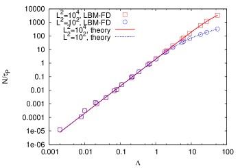
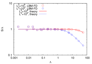
In figure 1 we present numerical simulations to benchmark these results. The numerical simulations have been carried out in three dimensional domains with cells. Periodic conditions are applied in the stream-flow (x) and in the transverse-flow (z) directions. The linear shear flow , is imposed in the LBM scheme by applying two opposite velocities in the stream-flow direction () at the upper () and lower wall () with the bounce-back rule Wolf-Gladrow (2001). We next change the shear in the range lbu and the polymer relaxation time in the range lbu for two values of the finite extensibility parameter, , and fixed lbu. In figure 1 we report the first normal stress difference (left panel) and the polymer shear viscosity (right panel), both rescaled with the viscosity , as a function of the dimensionless shear . The values of the conformation tensor are taken when the simulation has reached the steady state. All the numerical simulations collapse on different master curves, dependently on the value of . The normal stress difference increases at large to exhibit variable levels depending on , and consistently with the theoretical prediction of equation (30). The dependence of the normal stress from directly reflects in the presence of thinning effects visible in the plot of the polymer shear viscosity (see right panel of figure 1).
III.2 Steady Elongational Flow
We consider equation (24) under the effect of a steady elongational flow, , , , with the elongation rate. Again, writing out all the components we get
| (31) |
implying . Defining and , and introducing the dimensionless elongation rate , we find two independent equations for and
| (32) |
which can be rearranged to give us a cubic equation for as a function of . Such equation is most conveniently written as a quadratic equation in :
| (33) |
with associated solutions
| (34) |
where
| (35) |
The elongational viscosity
| (36) |
can be computed by numerically inverting equations (34-35) and paying attention to a proper selection of the sign in equation (34). For small the solution is given by , as is negative and divergent. The asymptotic expansion for small is indeed given by
| (37) |
showing that the elongational viscosity approaches a constant value at low elongation rates, which is three times the corresponding zero-shear-rate viscosity. However the radicand of equation (34) is zero when . In such a point, in order to preserve the continuity of the derivative of , we need to consider as a solution. Consistently, for large , we find
| (38) |
We therefore find the following asymptotic expansion for the elongational viscosity
| (39) |
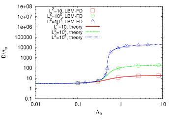
witnessing a divergence of the elongational viscosity in the Oldroyd-B limit (). In figure 2 we present numerical simulations to benchmark these results. The numerical simulations have been carried out in a three dimensional cubic domain with edge consisting of cells. Periodic conditions are applied in all directions. The elongational rate is changed in the range lbu and the polymer relaxation time in the range lbu, for three values of the finite extensibility parameter, , and fixed lbu. Again, the values of the conformation tensor are taken when the simulation has reached a steady state. When reporting the quantity , i.e. the elongational viscosity scaled by the polymer viscosity, as a function of the dimensionless elongational rate , all the numerical simulations collapse on different master curves, dependently on the value of . This behaviour is consistent with the theoretical predictions obtained from equations (34) and (35). For small the elongational viscosity is just three times the polymer viscosity, while at large we approach another constant value dependent on the finite extensibility parameter (see equation (39)).
III.3 Small amplitude Oscillatory Shearing
By promoting the shear variable considered in section (III.1) to a time-dependent variable, , , , we can analyze the behaviour of the polymer field under time-dependent loads. We will then analyze the limit of small amplitudes, i.e. . In this limit and we are left with the following time-dependent equation
| (40) |
For large , the equations for the first normal stress difference and polymer shear stress defined in section (III.1) are therefore
| (41) |
Assuming , we find that the stresses needed to maintain the motion will also be of oscillatory nature
where is the complex viscosity whose components can be computed by taking and as complex variables and considering the real and imaginary part of equation (41)
The dimensionless storage () and loss () moduli Bird et al. (1987) are given by
| (42) |
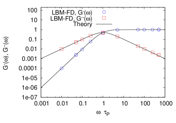
In figure 3 we present numerical simulations to benchmark these results. The set-up for the numerical simulations is similar to the one presented in section (III.1), with three dimensional domains consisting of cells, with variable wall-to-wall gap . We then apply an oscillatory shear flow , , at the walls of the LBM simulations and set zero feedback ( lbu) of the polymers into the fluid. The frequency is changed in the range lbu and the polymer relaxation time in the range lbu, for a given value of the finite extensibility parameter, , fixed lbu and maximum wall velocity lbu. A word of caution is in order, as the assumed flow conditions require that the lattice Boltzmann time to establish a steady shear flow, (with the solvent kinematic viscosity), is much shorter than the period of the oscillations, i.e. , otherwise the shear flow will be found in a transient regime. This condition is achieved by a proper tuning of the solvent kinematic viscosity and the wall gap in all the numerical simulations. As we can see from figure 3, the dimensionless storage modulus () and the dimensionless loss modulus () are in very good agreement with the theoretical prediction of equation (42).
III.4 Stress relaxation after cessation of steady shear flow
We finally consider a situation with , , with being constant for , and for . The equations for are therefore
| (43) |
We next write down the equations for the variables and
| (44) |
The first of equations (44) can be solved to get a differential equation for
| (45) |
where . The Oldroyd-B () limit simply implies an exponential decay , where with the subscript we indicate variables at time . For the general case with finite extensibility parameter in equation (45), cannot be written in terms of elementary functions. However, by a proper manipulations of equations (44), it is always possible to get an equation relating the shear stress to the trace of the stress during relaxation Bird et al. (1987)
| (46) |
For completeness, we note that further manipulations Bird et al. (1980); Herrchen and Oettinger (1997) of equations (44) allow to show that the area under the stress-relaxation curve is closely related to the first normal stress-difference before the cessation of the shear flow
| (47) |
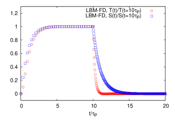
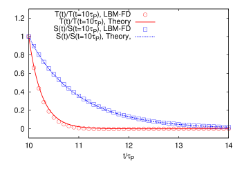
In the left panel of figure 4 we plot the time evolution for both and versus the dimensionless time () in the process of an inception of shear flow with the approaching to the steady state and subsequent cessation. The set-up for the numerical simulations is similar to the one presented in section (III.1), with three dimensional domains consisting of cells. The shear is set to lbu at time , with the polymer relaxation time lbu and finite extensibility parameter . The value of is chosen to create a net distinction between the time evolution of and , that otherwise would be identical in the Oldroyd-B limit (, see also equation (46)). The feedback of the polymer into the fluid is set to zero. For (that means in the above equations) the system is surely under the effect of a steady shear flow. At that time, the shear is suddenly switched off and the system starts decaying. The decay process is illustrated in the right panel of figure 4, where we compare the results of the numerical simulations with the analytical predictions obtained from equations (45) and (46).
IV Binary Mixtures with Viscoelastic Phases
In this section we describe problems where both phase segregation and viscoelasticity are present. First of all we switch on immiscibility: when in equation (6), with a critical value of the coupling constant, the binary mixture separates into two phases, each with a majority of one of the two components and with the interface between the two phases described as a thin layer of thickness across which the fluid properties change smoothly. The values of the interface thickness and the mobility (see equation (4)) need to be larger than those suggested by physical considerations in order to make the simulations affordable. They are empirically tuned in order to match the analytical predictions of sharp-interface hydrodynamics (see later).
We will then apply our numerical approach to the characterization of deformation of droplets in confined geometries, where the involved phases may possess a viscoelastic nature. This is a relevant problem, for example, when determining the properties of emulsions microstructures Christopher and Anna (2007); Seemann et al. (2012). Emulsions play an important role in a huge variety of applications, including foods, cosmetics, chemical and material processing Larson (1999). Deformation, break-up and coalescence of droplets occur during flow, and the control over these processes is imperative to synthesize the desired macroscopic behaviour of the emulsion. Most of the times, the synthesis of the emulsion takes place in presence of confinement, and relevant constituents have commonly a viscoelastic -rather than Newtonian- nature. The “single” drop problem has been considered to be the simplest model: in the case of dilute emulsions with negligible droplets interactions, the dynamics of a single drop indeed provides complete information about the emulsion behaviour. Single drop deformation has been extensively studied and reviewed in the literature for the case of Newtonian Taylor (1932); Grace (1982); Stone (1994); Rallison (1984) and also non-Newtonian fluids Greco (2002); Minale (2004); Minale et al. (2010); Guido (2011).
IV.1 Effects of confinement on droplet deformation
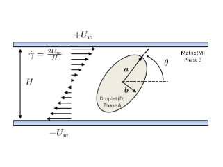
In the classical problem studied by Taylor Taylor (1932), a droplet with radius , interfacial tension , and viscosity is suspended in another immiscible fluid matrix with viscosity under the effect of a shear flow with intensity (see left panel of figure 5). The various physical quantities are grouped in two dimensionless numbers, the Capillary number
| (48) |
giving a dimensionless measure of the balance between viscous and interfacial forces, and the viscosity ratio , going from zero for vanishing values of the droplet viscosity (i.e. a bubble) to infinity in the case of a solid particle. In order to quantify the deformation of the droplet, we study the deformation parameter , where and are the droplet semi-axes in the shear plane, and the orientation angle between the major semi-axis and the flow direction (see also the left panel of figure 5). Taylor’s result, based on a small deformation perturbation analysis to first-order, relates the deformation parameter to the Capillary number ,
| (49) |
whereas the orientation angle is constant and equal to to first order. Taylor’s analysis was later extended by working out the perturbation analysis to second order in , which leaves unchanged the expression of the deformation parameter (49) and gives the correction to the orientation angle Rallison (1980); Chaffey and Brenner (1967). The effects of confinement have been theoretically addressed at by Shapira and Haber Shapira and Haber (1990); Sibillo et al. (2006) based on Lorentz’s reflection method. They found that the deformation parameter in a confined geometry can be obtained by the Taylor’s result through a correction in the power of the ratio between the droplet radius at rest and gap between the walls
| (50) |
where is a tabulated numerical factor depending on the relative distance between the droplet center and the wall (the value of for droplets placed halfway between the plates is ).
LBM have already been used to model the droplet deformation problems Xi and Duncan (1999); van der Sman and van der Graaf (2008); Komrakovaa et al. (2014); Liu and Zhang (2011). Three-dimensional numerical simulations of the classical Taylor’s problem Taylor (1932) have been performed by Xi & Duncan Xi and Duncan (1999) using the “Shan-Chen” model Shan and Chen (1993, 1994). The single droplet problem was also investigated by Van Der Sman & Van Der Graaf van der Sman and van der Graaf (2008) using a “free energy” LBM. LBM modelling of two phase flows is intrinsically a diffuse interface method and involves a finite thickness of the interface between the two liquids and related free-energy model parameters. These model parameters are characterized by two dimensionless numbers: the Péclet () and Cahn numbers (), the Cahn number is the interface thickness normalized with the droplet radius, whereas the Péclet number is the ratio between the convective time scale and the interface diffusion. A recent comprehensive study by Komrakova et al. has investigated the influence of , and mesh resolution on the accuracy and stability of the numerical simulations. Drops of moderate resolution (radius less than 30 lattice units) require smaller interface thickness, while a thicker interface should be used for highly resolved drops. Those parameters have to be within certain ranges to reproduce the physical behavior van der Sman and van der Graaf (2008); Komrakovaa et al. (2014) of sharp-interface hydrodynamics Magaletti et al. (2013). Since our aim is to quantify and explore the importance of viscoelasticity in our simulations, we choose the aforementioned parameters in such a way that the Newtonian (sharp-interface) predictions for droplet orientation and deformation are well reproduced. All the simulations described in the following sections refer to cases with polymer relaxation times ranging in the interval lbu and finite extensibility . The numerical simulations have been carried out in three dimensional domains with lattice cells. The droplet radius has been changed in the range lattice cells with fixed to achieve different confinement ratios . Periodic conditions are applied in the stream-flow (x) and in the transverse-flow (z) directions. The droplet is subjected to a linear shear flow , , with the shear introduced with two opposite velocities in the stream-flow direction () at the upper () and lower wall (). For the numerical simulations presented we have used lbu in (6) (the critical point is at for the parameters chosen) and a total average density of lbu, corresponding to a surface tension lbu and associated bulk densities lbu and lbu in the -rich region. Some numerical studies to test the sensitivity with respect to a change in the resolution and model parameters used are reported in A.
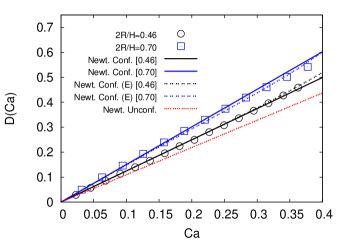
In the right panel of figure 5 we report the steady state deformation parameter for a Newtonian droplet under steady shear as a function of the associated Capillary number for two different confinement ratios: and . The viscosity ratio between the droplet phase and the matrix phase is fixed to , with the dynamic viscosities equal to lbu. The linearity of the deformation is captured by the numerical simulations up to the largest considered, but the numerical results overestimate Taylor’s prediction (referred to as “Newtonian Unconfined”) being well approximated by the theoretical prediction of Shapira & Haber for a confined droplet Shapira and Haber (1990) (refereed to as “Newtonian confined”). Confinement promotes larger deformation and wall effects act to stabilize the resulting elongated drop shapes (which would be otherwise unstable in the unbounded case) by confining the drop within closed streamlines Sibillo et al. (2006). For completeness, we also report a comparison with the steady state deformation prediction of a model proposed recently by Minale Minale (2008), describing the dynamics (and steady states) of a droplet under the assumption that it deforms into an ellipsoid. This model belongs to the family of “ellipsoidal” models Minale (2010b), which were originally introduced to describe the dynamics of a single Newtonian drop immersed in a matrix subjected to a generic flow field. The steady state predictions of such models for small are constructed in such a way to recover the exact perturbative result, i.e. Taylor’s result for an unbounded droplet Maffettone and Minale (1998) or the Shapira & Haber result for a confined droplet Minale (2008). The prediction of these ellipsoidal models is hardly distinguishable from the perturbative results Shapira and Haber (1990) in these Newtonian cases, at least for the range of parameters that we have used in the numerical simulations. Nevertheless, these models will be quite useful when discussing the influence of viscoelasticity on droplet deformation and orientation, as will be done in the following sections.
IV.2 Effects of Viscoelasticity on droplet deformation and orientation
In this section we look at the effects of viscoelasticity in droplet deformation and orientation. We will separately address the importance of matrix viscoelasticity and droplet viscoelasticity, using the proposed methodology described in section II, and compare with some of the theoretical predictions available in the literature Greco (2002); Minale (2004); Minale et al. (2010). Again, we work with unitary viscosity ratio, defined in terms of the total (fluid+polymer) shear viscosity: , in case of droplet viscoelasticity; , in case of matrix viscoelasticity. Viscoelastic effects show up in the droplet deformation and orientation in terms of two dimensionless parameters: the Deborah number,
| (51) |
where is the first normal stress difference generated in simple shear flow Bird et al. (1987), and the ratio between the second and first normal stress difference Greco (2002). Solving the constitutive equation for steady shear (see section (III.1)), the first normal stress difference for the FENE-P model Bird et al. (1987); Lindner et al. (2003) can be computed (see subsection (III.1) and equation (30)), while . In the Oldroyd-B limit () we can use the asymptotic expansion of the hyperbolic functions and we get so that
| (52) |
showing that is clearly dependent on the ratio between the polymer relaxation time and the emulsion time , the latter depending on the interface properties (i.e. surface tension). For finite , however, we need to use the definition of based on the first normal stress difference (see section (III.1)). Benchmark tests for the viscoelastic effects will be proposed for both shear-induced droplet deformation and orientation at small , although the effects on droplet orientation (especially in a case with matrix viscoelasticity) will be more pronounced. This is because non-Newtonian effects on the drop steady state deformation show up at the second order in , while the orientation angle has a correction at first order in Greco (2002); Guido (2011). In particular, to test both confinement and viscoelastic effects, we will also refer to the model proposed by Minale, Caserta & Guido Minale et al. (2010) for ellipsoidal droplets. Indeed, the aforementioned ellipsoidal models for Newtonian fluids have been recently proposed also for non-Newtonian fluids. In particular, Minale Minale (2004) proposed an ellipsoidal model which recovers, in the small -limit, the steady state theory developed by Greco Greco (2002). Minale, Caserta & Guido Minale et al. (2010) generalized the work by Minale Minale (2004, 2008) to study the effects of confinement in non-Newtonian systems.
We start with the effect of droplet viscoelasticity. For a given confinement ratio, , in figure 6 we report the steady state droplet deformation and orientation angle. We use the Oldroyd-B model, by choosing a large value of , and consider two relaxation times in the polymer equation (3), lbu and lbu, corresponding to Deborah numbers (based on equation (52)) and , respectively. The polymer viscosity is kept fixed to lbu, corresponding to a polymer concentration of . The deformation computed from the numerical simulations reveals a small effect of viscoelasticity, which is consistent with the theoretical prediction of the model by Minale, Caserta & Guido Minale et al. (2010) (referred to as ”non-Newtonian confined (E)”). In particular, with respect to the Newtonian case, deformation is slightly inhibited by viscoelasticity and overestimates Greco’s prediction for an unconfined non-Newtonian droplet Greco (2002) (referred to as “non-Newtonian unconfined”). As for the orientation, we again see a small effect. These observations echo other experimental and numerical results present in the literature on the effect of droplet viscoelasticity on deformation and orientation Verhulst
et al. (2009a, b); Aggarwal and Sarkar (2007, 2008).
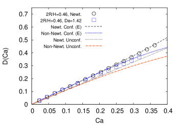
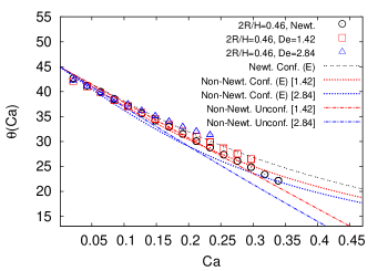
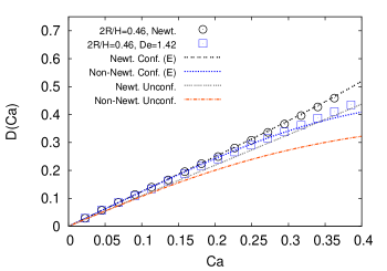
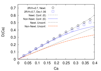
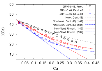
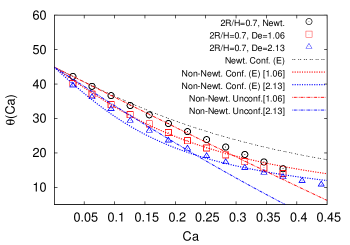
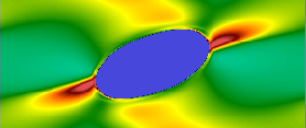
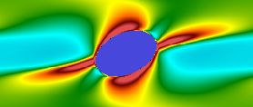
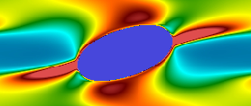
We next look at the effect of matrix viscoelasticity, figures 7 and 8. In figure 7 we report the steady state droplet deformation for two different confinement ratios: (left panel) and (right panel). Again, we choose a large value of , and consider a relaxation time lbu in the polymer equation (3), corresponding to different Deborah numbers, depending on the droplet radius (see equation (52)): for and for . The polymer viscosity is kept fixed to lbu, corresponding to a polymer concentration of . In both cases, matrix viscoelasticity inhibits droplet deformation with respect to the corresponding Newtonian cases. Also, the unconfined theory by Greco Greco (2002) underestimates the deformation, and the mismatch is larger with the larger confinement ratio, as one would have expected since the theory of Greco does not take into account confinement. The model by Minale, Caserta & Guido Minale et al. (2010) follows the numerical data with a mismatch emerging at large for the larger confinement ratio: most probably this is due to the fact that confinement starts to act in promoting deformation with shapes departing from an ellipsoid Sibillo et al. (2006). A non trivial interplay between confinement and viscoelasticity is also visible from figure 9, where we report the steady state snapshots for the polymer feedback stress of equation (2) for the cases studied in figures 7 and 8. In figure 8 we report the orientation angle for the same cases studied in figure 7. The effect of viscoelasticity is now much more visible, if compared with the case of droplet viscoelasticity reported in figure 6. We also analyze the effect of an increase of the relaxation time in equation (3) for both the confinement ratios studied, which translates in a larger Deborah number. The change in the orientation angle for the Newtonian cases is linear in up to the largest considered, which is consistent with the linearity of the deformation discussed in figure 5. This generates a mismatch with the corresponding Ellipsoidal model predictions Minale (2008): just to give some quantitative numbers, for a Capillary number , there is a mismatch of in the smaller confinement ratio, which becomes roughly doubled (i.e. ) for the larger confinement ratio. The orientation angle in the non-Newtonian cases, instead, is better captured by the ellipsoidal model by Minale, Caserta & Guido Minale et al. (2010). Overall, in both the Newtonian and non-Newtonian cases, the mismatch between the numerical results and the prediction of the ellipsoidal models is more pronounced at large confinement ratios (right panel of figure 8), an observation that echoes the discussion done for the data of figure 7.


.
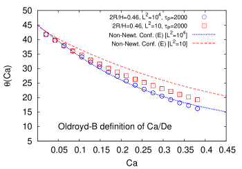
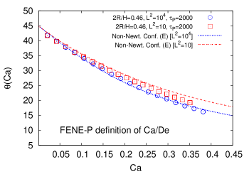
Finally, we want to address and test the importance of the finite extensibility parameter in the polymer equation (3). For a given confinement ratio and lbu in equation (3), we have repeated the numerical simulations described in the left panel of figure 7 for a finite extensibility parameter . As decreases, the polymer dumbell becomes less extensible and the maximum level of stress attainable is reduced. There are some consequences. First, we cannot rely on equation (52) to define the Deborah number, which strictly holds only in the large- limit. Second, at large shears, the model exhibits thinning effects, as predicted and verified in subsection (III.1), and the definition of the Capillary number (48) given in terms of the matrix viscosity has to be changed to include such effects. Indeed, by using the definition of the Deborah number given in equation (52) and a shear independent matrix viscosity in equation (48) in the theoretical models, the agreement between the numerical results and the theory deteriorates (see left panel of figure 10), whereas the large- case was well in agreement. In the right panel of figure 10 we report the same data, by changing: (i) the definition of Capillary in equation (48), based on the thinning effects analyzed in subsection (III.1); (ii) the definition of the Deborah number, which is now computed according to equation (51), with the first normal stress difference given in (30). As one can see the agreement gets better, especially at small . For completeness, in figure 11, we report the steady state snapshots for the polymer feedback stress of equation (2) for the cases studied in figure 10. Results reported in figure 10 are surely motivating for future theoretical studies. Indeed, it is by no means proved that the theoretical models used Minale et al. (2010) can work for a shear-dependent viscosity (which holds for the FENE-P). Figure 10 is giving (numerical) evidence that the viscoelastic effects of the FENE-P model can also be embedded in such theoretical models; however, before proceeding with further comparisons, we feel that a proper theoretical background needs to be developed first.


.
V Conclusions
We have proposed numerical simulations of viscoelastic fluids based on a hybrid algorithm combining lattice-Boltzmann models (LBM) and Finite Differences (FD) schemes, the former used to model the macroscopic hydrodynamic equations, and the latter used to model the kinetics of polymers using the constitutive equations for finitely extensible non-linear elastic dumbells with Peterlin’s closure (FENE-P). We have first benchmarked the numerical scheme with the characterization of the rheological properties of a dilute homogeneous solution under steady shear, steady elongational flows, oscillatory flows and transient shear. We then continued to study the model in presence of non-ideal multicomponent interfaces, where immiscibility is introduced in the LBM description using the “Shan-Chen” interaction model Shan and Chen (1993, 1994); Benzi et al. (2009). We have characterized the effect of viscoelasticity in droplet deformation under steady shear, by comparing the results of numerical simulations with available theoretical models in the literature Greco (2002); Minale (2004); Shapira and Haber (1990); Minale (2008); Minale et al. (2010); Minale (2010a); Taylor (1932). Overall, the numerical simulations well capture both the effects of confinement and viscoelasticity, thus exploring problems where the capabilities of LBM were never quantified before. Even if we focused on a unitary total (Newtonian fluid+polymer) viscosity ratio, the numerical algorithm can simulate viscosity ratios different from as well, although we think that the latter cannot easily be pushed much below and much above . Based on the total shear viscosity, we actually show in this paper that there is a good matching between the analytical solutions and the numerical results for those cases where the viscosity ratio between the two Newtonian phases is between and , while keeping the total (Newtonian fluid+Polymer) viscosity ratio equal to . We think the good matching is possible only because the “bare” Newtonian solution is recovered, therefore lending support to the validity of the algorithm in simulating viscosity ratios different from . As an upgrade of complexity, it would be extremely interesting to study time-dependent situations Verhulst et al. (2009b); Cardinaels and Moldenaers (2010), other flows in confined geometries Arratia et al. (2009); Derzsi et al. (2013) and problems where droplet break-up is involved Cardinaels et al. (2011); Gupta and Sbragaglia (2014). Complementing these kind of experimental results with the help of numerical simulations would be of extreme interest. Simulations provide easy access to quantities such as drop deformation and orientation as well as the velocity flow field, pressure field, and polymers feedback stresses, inside and outside the droplet. They can be therefore useful to perform in-silico comparative studies, at changing the model parameters, to shed lights on the complex properties of viscoelastic flows in confined geometries.
VI Acknowledgements
The authors kindly acknowledge funding from the European Research Council under the European Community’s Seventh Framework Programme (FP7/2007-2013)/ERC Grant Agreement no[279004]. We also acknowledge L. Biferale and R. Benzi for useful discussions. A. Gupta acknowledges R. Pandit and S. S. Ray for useful discussions during his visits to IISc Bangalore (February 2014) and ICTS-TIFR Bangalore (October 2013).
Appendix A Sensitivity with respect to a change in the resolution and model parameters used
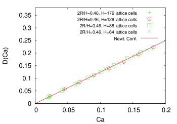
The convergence towards the sharp-interface limit of hydrodynamics is one of the crucial issues in diffuse interface models van der Sman and van der Graaf (2008); Komrakovaa et al. (2014); Magaletti et al. (2013); Khatavkar et al. (2006); Lowengrub and Truskinowsky (1998). In the present work, the resolution used, the interface thickness, the mobility were all empirically tuned in order to match the analytical predictions of sharp-interface (Newtonian) hydrodynamics. In this Appendix we provide evidence that the chosen parameters lie in a range of values where the hydrodynamic solution is indeed well recovered. The reference numerical data are those analyzed in the right panel of figure 5 for . The sensitivity with respect to a change in the resolution used is tested by keeping all the parameters fixed, except the wall-to-wall gap and the radius , which are changed in the ranges lattice cells and lattice cells, in such a way to keep fixed the confinement ratio to . All the numerical simulations performed match very well with the theoretical prediction of Shapira & Haber for a confined Newtonian droplet Shapira and Haber (1990) (referred to as “Newtonian confined”). Even the simulations with the smallest radius analyzed ( lattice cells) are well in agreement with the theoretical predictions, a fact that is also acknowledged in other publications using the “Shan-Chen” interaction model Onishi et al. (2006).
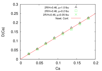
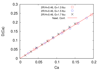
We next continue by performing numerical simulations to test the sensitivity with respect to a change in the mobility (see (4)-(16)) and in the interface width. In both cases, again, the reference numerical data are those analyzed in the right panel of figure 5 for , corresponding to a mobility lbu and interface width approximately equal to lattice cells. In a series of numerical simulations, we change the mobility in the range lbu, by keeping all the other parameters unchanged. Results are reported in the left panel of figure 13, showing no remarkable sensitivity, at least as far as the deformation parameter is concerned. In a second set of numerical simulations, we keep the mobility fixed to lbu and change the interface width: the interaction parameter is changed in the range lbu at fixed total average density, resulting in surface tensions varying in the range lbu. The interface widths are changed in a range between lattice cells and lattice cells approximately (wider interfaces are obtained with smaller ). The associated bulk densities change in the range lbu and lbu in the -rich region. For each value of , we define the Capillary number according to (48), dependently on the value of the surface tension. The results for the deformation parameter as a function of the Capillary number are reported in the right panel of figure 13, confirming that the parameters used in our study lie in a range where the convergence towards the sharp-interface limit of hydrodynamics is well achieved.
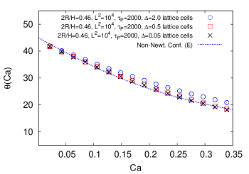
We finally address the importance of the smoothing parameter for the viscoelastic properties (19). We choose the data analyzed in the left panel of figure 8 for the Deborah number . The smoothing parameter is changed in the range lattice cells and results are reported in figure 14. As expected, for values of below 1 lattice cell, the results are all well in agreement withe the reference theory of sharp-interface hydrodynamics. Deviations start to emerge when the smoothing parameter is above a lattice cell.
Appendix B Comparison with the Model by Onishi et. al.
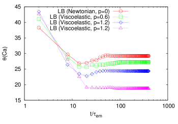
In this Appendix we compare the results of our model with those of Onishi et al. Onishi et al. (2006). The two approaches are intrinsically different with regard to the modelling of the polymer dynamics: Onishi et al. use an approach based on the Fokker-Planck equation (simulated with LBM), whereas we directly model the conformation tensor dynamics (with FD), which comes from a proper closure of the Fokker-Planck equation Bird et al. (1987); Herrchen and Oettinger (1997). Comparing the two theoretical formulations is outside the scope of our paper, and surely addressed in many other dedicated works Bird et al. (1987); Herrchen and Oettinger (1997). The comparison between the two models can be fairly addressed, at least as far as it concerns the solvent part of the model, which is done with LBM in both cases. We do not propose anything new in this direction, since we use the MRT, whose advantages with respect to the single time BGK relaxation approximation (used by Onishi et al. Onishi et al. (2006)) are well known from the literature Yu and Fan (2010); d’Humières et al. (2002). These facts said, from the information provided in the paper by Onishi et al. Onishi et al. (2006), we could run numerical simulations to compare with the results there reported. We perform numerical simulations in three dimensional domains with lattice cells and droplet radius lattice cells, which is the same resolution used by Onishi et al. in their paper Onishi et al. (2006). Exactly as in Onishi et al. (2006), we prepare four fluids with viscoelasticity in the matrix phase: the matrix viscosity is kept the same, lbu, but different viscoelastic properties are considered: and (run M1 in Onishi et al. (2006), the Newtonian case); and (run M2 in Onishi et al. (2006)); and (run M3 in Onishi et al. (2006)); and (run M4 in Onishi et al. (2006)). In all cases, the mobility in (16) is set to lbu. In figure 15, similarly to figure 3 of Onishi et al. Onishi et al. (2006), we begin with the presentation of the temporal evolution of Taylor’s deformation parameter and orientation angle obtained in runs M1-M4 for a fixed Capillary number . To be noted that the Deborah number is denoted with in Onishi et al. (2006): we therefore decided to use to better (visually) establish a link with the results of Onishi et al. (2006). In agreement with Onishi et al. (2006), there is no remarkable difference in the approach to steady state, though overshoots are a bit more pronounced in our case. Note that we have made time dimensionless with respect to the droplet emulsion time , whereas it is not clearly stated what is the characteristic time scale used by the authors in Onishi et al. (2006). In agreement with the theory, the deformation parameter only slightly changes at changing the degree of viscoelasticity whereas the orientation angle is more sensitive.
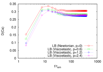
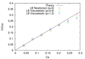
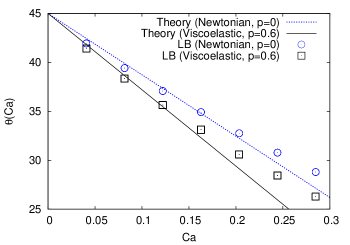
Next, we compare the steady state shape of the drops in the different matrices in order to investigate viscoelasticity effects. Figures 16 are the counterpart of figure 5 in Onishi et al. (2006): they report the steady state values of the deformation parameter and the orientation angle for different Capillary numbers. Note that the resolution used is already enough to achieve convergence to the hydrodynamic limit (see figure 12). Indeed, in agreement with Onishi et al. (2006), the quantitative matching with the theoretical prediction by Greco Greco (2002) is achieved.
References
References
- Benzi et al. (1992) R. Benzi, S. Succi, and M. Vergassola, Physics Reports 222, 145 (1992).
- Succi (2001) S. Succi, The Lattice Boltzmann Equation for Fluid Dynamics and Beyond (Oxford University Press, 2001).
- Wolf-Gladrow (2001) D. Wolf-Gladrow, Lattice-Gas Cellular Automata and Lattice Boltzmann Models: An Introduction (Springer Verlag, 2001).
- Chen and Doolen (1998) S. Chen and G. D. Doolen, Annu. Rev. Fluid Mech. 30, 329 (1998).
- Aidun and Clausen (2010) C. K. Aidun and J. R. Clausen, Annu. Rev. Fluid Mech. 42, 439 (2010).
- Zhang (2011) J. Zhang, Microfluid Nanofluid 10, 1 (2011).
- Shan and Chen (1993) X. Shan and H. Chen, Phys. Rev. E 47, 1815 (1993).
- Shan and Chen (1994) X. Shan and H. Chen, Phys. Rev. E 49, 2941 (1994).
- Biferale et al. (2012) L. Biferale, P. Perlekar, M. Sbragaglia, and F. Toschi, Phys. Rev. Lett. 108, 104502 (2012).
- Sbragaglia et al. (2012) M. Sbragaglia, R. Benzi, M. Bernaschi, and S. Succi, Soft Matter 8, 10773 (2012).
- Sega et al. (2013) M. Sega, M. S. S. S. Kantorovich, and A. O. Ivanovd, Soft Matter 9, 10092 (2013).
- Gross et al. (2011) M. Gross, M. E. Cates, F. Varnik, and R. Adhikari, Journal of Statistical Mechanics: Theory and Experiment p. P03030 (2011).
- Dünweg et al. (2008) B. Dünweg, U. D. Schiller, and A. J. Ladd, Computer Physics Communications 180, 605 (2008).
- Kaehler and Wagner (2013) G. Kaehler and A. J. Wagner, Phys. Rev. E 87, 063310 (2013).
- Larson (1999) R. G. Larson, The Structure and Rheology of Complex Fluids (Oxford University Press, 1999).
- Peterlin (1961) A. Peterlin, Polymer 2, 257 (1961).
- Bird et al. (1987) R. B. Bird, R. C. Armstrong, and O. Hassager, Dynamics of polymeric liquids (J. Wiley & Sons, 1987).
- Oldroyd (1950) J. G. Oldroyd, Proc. R. Soc. London, Ser. A 200, 523 (1950).
- Vaithianathan and Collins (2003) T. Vaithianathan and L. R. Collins, Journal Computational Physics 187, 1 (2003).
- Tomé et al. (2007) M. Tomé, L. Grossi, A. Castelo, J. Cuminato, S. McKee, and K. Walters, J. Non-Newtonian Fluid Mech. 141, 148 (2007).
- Oliveira (2001) P. J. Oliveira, J. Non-Newtonian Fluid Mech. 101, 113 (2001).
- Yue et al. (2004) P. Yue, J. J. Feng, C. Liu, and J. Shen, J. Fluid Mech. 515, 293 (2004).
- Yue et al. (2005) P. Yue, J. J. Feng, C. Liu, and J. Shen, J. Fluid Mech. 540, 427 (2005).
- Purnode and Crochet (1998) B. Purnode and M. J. Crochet, J. Non-Newtonian Fluid Mech. 77, 1 (1998).
- Chauviére and Owens (2000) C. Chauviére and R. G. Owens, J. Non-Newtonian Fluid Mech. 95, 1 (2000).
- Qian and Deng (1997) Y. H. Qian and Y.-F. Deng, Phys. Rev. Lett. 79, 2742 (1997).
- Ispolatov and Grant (2002) I. Ispolatov and M. Grant, Phys. Rev. E 65, 056704 (2002).
- Giraud et al. (1997) L. Giraud, D. d’Humiéres, and P. Lallemand, Int. J. Mod. Phys. C 8, 805 (1997).
- Giraud et al. (1998) L. Giraud, D. d’Humiéres, and P. Lallemand, Europhys. Lett. 42, 625 (1998).
- Lallemand et al. (2003) P. Lallemand, D. d’Humiéres, L.-S. Luo, and R. Rubinstein, Phys. Rev. E 67, 021203 (2003).
- Malaspinas et al. (2010) O. Malaspinas, N. Fiétier, and M. Deville, J. Non-Newtonian Fluid Mech. 165, 1637 (2010).
- Denniston et al. (2001) C. Denniston, E. Orlandini, and J. M. Yeomans, Phys. Rev. E 63, 056702 (2001).
- Marenduzzo et al. (2007) D. Marenduzzo, E. Orlandini, M. E. Cates, and J. M. Yeomans, Phys. Rev. E 76, 031921 (2007).
- Onishi et al. (2005) J. Onishi, Y. Chen, and H. Ohashi, Prog. Comp. Fluid Dyn. 5, 75 (2005).
- Onishi et al. (2006) J. Onishi, Y. Chen, and H. Ohashi, Physica A 362, 84 (2006).
- Singh et al. (2013) S. Singh, G. Subramanian, and S. Ansumali, Phys. Rev. E 88, 013301 (2013).
- Pham et al. (2009) T. T. Pham, U. D. Schiller, J. R. Prakash, and B. Dünweg, Journal of Chemical Physics 131, 164114 (2009).
- Gunstensen et al. (1991) A. E. Gunstensen, D. H. Rothman, and S. Zaleski, Phys. Rev. A 43, 4320 (1991).
- Liu et al. (2012) H. Liu, A. J. Valocchi, and Q. Kang, Phys. Rev. E 85, 046309 (2012).
- Benzi et al. (2009) R. Benzi, M. Sbragaglia, S. Succi, M. Bernaschi, and S. Chibbaro, Jour. Chem. Phys. 131, 104903 (2009).
- Swift et al. (1996) M. R. Swift, E. Orlandini, W. R. Osborn, and J. M. Yeomans, Phys. Rev. E 54, 5041 (1996).
- Greco (2002) F. Greco, J. Non-Newtonian Fluid Mech. 107, 111 (2002).
- Minale (2004) M. Minale, J. Non-Newtonian Fluid Mech. 123, 151 (2004).
- Shapira and Haber (1990) M. Shapira and S. Haber, Int J Multiph Flow 16, 305 (1990).
- Minale (2008) M. Minale, Rheol. Acta 47, 667 (2008).
- Minale et al. (2010) M. Minale, S. Caserta, and S. Guido, Langmuir 26, 126 (2010).
- Minale (2010a) M. Minale, Rheol Acta 49, 789 (2010a).
- Sbragaglia and Belardinelli (2013) M. Sbragaglia and D. Belardinelli, Phys. Rev. E 88, 013306 (2013).
- Premnath and Abraham (2007) K. Premnath and J. Abraham, Journal of Computational Physics 224, 539 (2007).
- Porter et al. (2012) M. L. Porter, E. T. Coon, Q. Kang, J. D. Moulton, and J. W. Carey, Phys. Rev. E 86, 036701 (2012).
- Dünweg et al. (2007) B. Dünweg, U. D. Schiller, and A. J. C. Ladd, Phys. Rev. E 76, 036704 (2007).
- Perlekar et al. (2006) P. Perlekar, D. Mitra, and R. Pandit, Phys. Rev. Lett. 97, 264501 (2006).
- Scarbolo et al. (2013) L. Scarbolo, D. Molin, P. Perlekar, M. Sbragaglia, A. Soldati, and F. Toschi, Journal of Computational Physics 234, 263 (2013).
- Bird et al. (1980) R. Bird, P. Dotson, and R. Armstrong, Journal of Non-Newtonian Fluid Mechanics 7, 213 (1980).
- Herrchen and Oettinger (1997) M. Herrchen and H. Oettinger, J. Non-Newtonian Fluid Mech. 68, 17 (1997).
- Lindner et al. (2003) A. Lindner, J. Vermant, and D. Bonn, Physica A 319, 125 (2003).
- Christopher and Anna (2007) G. F. Christopher and S. L. Anna, J Phys D Appl Phys 40, R319 (2007).
- Seemann et al. (2012) R. Seemann, M. Brinkmann, T. Pfohl, and S. Herminghaus, Rep. Prog. Phys. 75, 016601 (2012).
- Taylor (1932) G. I. Taylor, Proc. Royal Soc A 138 (1932).
- Grace (1982) H. P. Grace, Chem. Eng. Commun. 14, 225 (1982).
- Stone (1994) H. A. Stone, Annu. Rev. Fluid Mech. 26, 65 (1994).
- Rallison (1984) J. M. Rallison, Annu. Rev. Fluid Mech. 16, 45 (1984).
- Guido (2011) S. Guido, Current Opinion in Colloid & Interface Science 16, 61 (2011).
- Rallison (1980) R. J. Rallison, Jour. Fluid Mech. 98, 625 (1980).
- Chaffey and Brenner (1967) C. E. Chaffey and H. Brenner, J Colloid Interface Sci. 24, 258 (1967).
- Sibillo et al. (2006) V. Sibillo, G. Pasquariello, M. Simeone, V. Cristini, and S. Guido, Phys. Rev. Lett. 97, 054502 (2006).
- Xi and Duncan (1999) H. Xi and C. Duncan, Phys. Rev. E 59, 3022 (1999).
- van der Sman and van der Graaf (2008) R. G. M. van der Sman and S. van der Graaf, Comput. Phys. Commun. 178, 492 (2008).
- Komrakovaa et al. (2014) A. E. Komrakovaa, O. Shardt, D. Eskinb, and J. J. Derksen, International Journal of Multiphase Flow 59, 23 (2014).
- Liu and Zhang (2011) H. Liu and Y. Zhang, Phys. Fluids 23, 082101 (2011).
- Magaletti et al. (2013) F. Magaletti, F. Picano, M. Chinappi, L. Marino, and C. M. Casciola, Jour. Fluid Mech. 714, 95 (2013).
- Minale (2010b) M. Minale, Rheol. Acta 49, 789 (2010b).
- Maffettone and Minale (1998) P. L. Maffettone and M. Minale, J. Non Newton. Fluid Mech 78, 227 (1998).
- Verhulst et al. (2009a) K. Verhulst, R. Cardinaels, P. Moldenaers, Y. Renardy, and S. Afkhami, J. Non-Newt. Fluid Mech. 156, 29 (2009a).
- Verhulst et al. (2009b) K. Verhulst, R. Cardinaels, P. Moldenaers, S. Afkhami, and Y. Renardy, J. Non-Newt. Fluid Mech. 156, 44 (2009b).
- Aggarwal and Sarkar (2007) N. Aggarwal and K. Sarkar, J. Fluid Mech. 584, 1 (2007).
- Aggarwal and Sarkar (2008) N. Aggarwal and K. Sarkar, J. Fluid Mech. 601, 63 (2008).
- Cardinaels and Moldenaers (2010) R. Cardinaels and P. Moldenaers, Rheologica acta 49, 941 (2010).
- Arratia et al. (2009) P. E. Arratia, L.-A. Cramer, J. P. Gollub, and D. J. Durian, New J. Phys. 11, 115006 (2009).
- Derzsi et al. (2013) L. Derzsi, M. Kasprzyk, J.-P. Plog, and P. Garstecki, Phys. Fluids 25, 092001 (2013).
- Cardinaels et al. (2011) R. Cardinaels, A. Vananroye, P. Van Puyvelde, and P. Moldenaers, Macromolecular Materials and Engineering 296, 214 (2011).
- Gupta and Sbragaglia (2014) A. Gupta and M. Sbragaglia, Phys. Rev. E 90, 023305 (2014).
- Khatavkar et al. (2006) V. Khatavkar, P. Anderson, and H. Meijer, Chemical Engineering Science 61, 2364 (2006).
- Lowengrub and Truskinowsky (1998) J. Lowengrub and L. Truskinowsky, Proc. R. Soc. Lond. A 454, 2617 (1998).
- Yu and Fan (2010) Z. Yu and L.-S. Fan, Phys. Rev. E 82, 046708 (2010).
- d’Humières et al. (2002) D. d’Humières, I. Ginzburg, M. Krafczyk, P. Lallemand, and L.-S. Luo, Phil. Trans. Roy. Soc. London 360, 437 (2002).