IFJPAN-IV-2014-1 Monte Carlo study of NLO correction to QCD evolution kernel induced by the change of the factorization scale

Abstract

The aim of the present study is to show that: the redefinition of the factorization scale $Q_{i}\to z_{i}Q_{i}$ in the ladder can be traded exactly for the NLO correction to the LO evolution kernel, $P(z)\to P(z)+(2C_{F}\alpha_{S}/\pi)\Delta(z)$ The above observation was done/exploited in the literature, but the present study demonstrates how this phenomenon is realized within the Markovian Monte Carlo parton shower – hence it might be relevant in MC practice.

12.38.-t, 12.38.Bx, 12.38.Cy

1 Introduction

In the collinear factorization the factorization scale $Q$ limits transverse phase space of all emitted particles. Typical practical choices of $Q$ are: virtuality of the emiter parton at the end of the multiple emission process, maximum transverse momentum or maximum rapidity of all emitted partons, $\mu_{F}$ of the dimensional regularization, total energy in the hard process $\sqrt{\hat{s}}$, etc. Redefinition of the factorization scale may involve factor $z$ being the relative loss of the energy of the emitter: $Q\to z^{\sigma}Q$, $z=x_{n}/x_{0}$, $\sigma=\pm 1,\pm 2$. Many examples can be found in the literature, for instance: (i) change from $\mu_{F}$ to virtuality in the hard process coefficient function  [1], (ii) change from time-like to space-like ladder in the Curci-Furmanski-Petronzio (CFP) calculation of NLO kernels [2], (iii) change from angular- to kT-ordering in the modelling of low $x$ structure function by Catani-Ciafaloni-Fiorani-Marchesini (CCFM) [3].

The aim of the present study is to show that: the redefinition of the factorization scale $Q\to z^{\sigma}Q$ in the ladder can be traded exactly for the NLO correction to the LO evolution kernel, $P(z)\to P(z)+\sigma(2C_{F}\alpha_{S}/\pi)\Delta(z)$. Without loss of generality, in the numerical exercise we shall opt for $\sigma=1$. As already said, the above observation was already done/exploited in the literature. Here, the above mechanism will be demonstrated numerically, in a form which can be useful in the construction of the Monte Carlo parton shower with the built in NLO evolution of the showers [4].

2 Simplified DGLAP evolution in the Markovian Monte Carlo form

For our numerical exercise we shall use simplified DGLAP evolution in the Markovian Monte Carlo form. We consider an incoming quark which emits gluons, before it enter hard process. Its energy distribution $D(T,x)$ is a function of the evolution time $T=\ln Q^{2}$. The DGLAP evolution equation  [5] reads:

$$\frac{\partial}{\partial T}D(T,x)=\frac{2\alpha_{s}(T)}{\pi}\int_{x}^{1}\frac{dz}{z}P(z)D\Big{(}T,\frac{x}{z}\Big{)}=\frac{2\alpha_{s}(T)}{\pi}\Big{[}P(\cdot)\otimes D(T,\cdot)\Big{]}(x)$$ (2.1)

where $x$ is a part of initial energy (more precisely lightcone variable) left after the emissions of a gluon from a quark. The running QCD coupling constant is $\alpha_{s}(T)=4\pi/(2\beta_{0}(T-\ln\Lambda_{0}))$ [6] where $\beta_{0}$ is that of ref. [7] and $\Lambda_{0}$ is the QCD scale parameter. However, for the sake of simplicity we shall adopt constant $\alpha_{s}$ in the following numerical exercises. The evolution kernel $P(z)$ is given by:

$$\begin{split}&P(z)=C_{F}\bigg{\{}\frac{1+z^{2}}{2(1-z)_{+}}+\frac{3}{4}\delta(1-z)\bigg{\}}=-P^{\delta}(\epsilon)\delta(1-z)+P^{\theta}(\epsilon,z),\end{split}$$ (2.2)

where:

$$\begin{split}&P^{\theta}(\epsilon,z)=\frac{C_{F}}{2}\frac{1+z^{2}}{1-z}\theta(1-z-\epsilon),\quad\\ &P^{\delta}(\epsilon)=\int_{0}^{1}dz\;P^{\theta}(\epsilon,z)=C_{F}\left[\ln\left(\frac{1}{\epsilon}\right)-\frac{3}{4}\right],\end{split}$$ (2.3)

$\epsilon\rightarrow 0$ is an infrared regulator and $C_{F}=\frac{3}{4}$ is the colour-group factor. $P^{\delta}(\epsilon)$ is deliberately chosen to be positive – it is uniquely determined from the baryon number conservation condition, $\int_{0}^{1}dz\;P(z)=0.$

Figure 2.1: The $\Delta$-function of Curci–Furmanski–Petronzio.

The iteration of the above evolution equation leads to the following solution:

$$\begin{split}&D(T,x)=e^{-\Phi(T,t_{0})}D(t_{0},x)+\\ &+\sum_{n=1}^{\infty}\int_{t_{0}}^{T}\prod_{i=1}^{n}\bigg{[}dt_{i}\theta(t_{i}-t_{i-1})\bigg{]}e^{-\Phi(T,t_{n})}\times\\ &\times\prod_{j=1}^{n}\bigg{[}\frac{2\alpha_{s}(t_{j})}{\pi}\;P^{\theta}(\epsilon,\cdot)e^{-\Phi(t_{j},t_{j-1})}\otimes\bigg{]}D(t_{0},\cdot)(x),\end{split}$$ (2.4)

where the Sudakov form-factor $\Phi(T,t_{0})$ is given by $\Phi(T,t_{0})=\int_{t_{0}}^{T}dt^{\prime}\;\frac{2\alpha_{s}(t^{\prime})}{\pi}\;P^{\delta}(\epsilon).$

On the other hand, the exact solution of the evolution equation for $D(T,x)$ can be obtained with high numerical precision from the Markovian Monte Carlo program. The probability distribution for generating single Markovian step forward, that is generating the next $(t,x)$ starting from the previous $(t_{0},x_{0})$, is given by:

$$\begin{split}&p(t,x|t_{0},x_{0})=\theta(t-t_{0})\frac{2\alpha_{s}(t)}{\pi}P^{\theta}\left(\epsilon,\frac{x}{x_{0}}\right)e^{-\Phi(t,t_{0})},\quad\\ &\int_{t_{0}}^{\infty}dt\int_{0}^{x_{0}}dx\;p(t,x|t_{0},x_{0})=1.\end{split}$$ (2.5)

Our toy model Markovian Monte Carlo algorithm works as follows:

• $x_{0}$ is generated according to $D(x_{0})=3(1-x_{0})^{2}$,  $\int_{0}^{1}dx_{0}\;D(x_{0})=1$.

• $t_{i}=\ln(Q_{i})$ and $z_{i}=\frac{x_{i}}{x_{i-1}}$ are generated in a loop according to $p(t_{i},x_{i}|t_{i-1},x_{i-1})$ for $i=1,2,3,...$

• Markovian process (loop) is terminated at $i=N$, when $t_{N+1}>T$ for the first time.

• The above procedure is repeated many times and the resulting distribution of the final $x=x_{N}$ will be distributed according to $D(T,x)$ being the solution of the evolution equation, see ref. [8] for more details.

2.1 The $\Delta$-function of CFP

In the perturbative QCD the evolution kernel $P(z)$ is calculable order by order:

$$P(\alpha_{s},z)=P^{(0)}(z)+\Big{(}\frac{\alpha_{s}}{2\pi}\Big{)}^{1}P^{(1)}(z)+\Big{(}\frac{\alpha_{s}}{2\pi}\Big{)}^{2}P^{(2)}(z)+...,$$ (2.6)

where $P^{(0)}(z)$, $P^{(1)}(z)$ and $P^{(2)}(z)$ are the leading (LO), next-to-leading (NLO) and next-to-next-to-leading order (NNLO) approximations respectively. LO kernels are known since DGLAP works [5], while NLO kernels were obtained directly from the Feynman diagrams in ref. [2]. In the same ref. [2] it was noticed that NLO corrections to the kernels for the initial state ladder differ from the ones for final state by $\big{(}\frac{\alpha_{s}}{2\pi}\big{)}C_{F}^{2}\Delta(z)$ where

$$C_{F}^{2}\Delta(z)=\left[P^{(0)}(\cdot)\otimes\left(\ln(\cdot)\;P^{(0)}(\cdot)\right)\right](z)$$ (2.7)

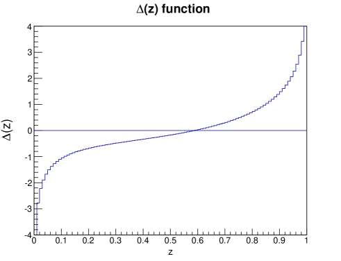
and the LO kernel $P^{(0)}(z)=P(z)$ is that of eq. (2.2). The above $\Delta$-function is easily calculable:

$$\begin{split}&\Delta(z)=\int_{0}^{1}dx\;\bigg{\{}\frac{\theta(x>z)}{x}\frac{1+x^{2}}{2(1-x)}\;\ln(y)\frac{1+y^{2}}{2(1-y)}\bigg{|}_{y=z/x}\\ &~{}~{}~{}~{}~{}~{}~{}~{}~{}~{}~{}~{}~{}~{}~{}~{}~{}~{}~{}~{}~{}~{}~{}~{}~{}-\frac{1+x^{2}}{2(1-x)}\;\ln(y)\frac{1+y^{2}}{2(1-y)}\bigg{|}_{y=z}\bigg{\}}\\ &~{}~{}~{}~{}~{}~{}~{}=\frac{1+z^{2}}{2(1-z)}\ln z\left[\ln\frac{(1-z)^{2}}{z}+\frac{3}{2}\right]+\frac{1+z}{8}\ln^{2}z-\frac{1-z}{4}\ln z,\end{split}$$ (2.8)

This function is visualised in Figure 2.1. It obeys the sum rule $\int_{0}^{1}dz\;\Delta(z)=0$ due to $\int_{0}^{1}P^{(0)}(z)dz=0$.

3 $\Delta$-function of CFP in the framework of Markovian MC

In the following we are going to show with the help of the Markovian Monte Carlo that the change of the time limit from $T$ to $(T+\ln x)$ induces a NLO correction to the evolution kernel being $C_{F}^{2}\frac{\alpha_{s}}{\pi}\Delta(z)$.

In the CFP work the $\Delta$-function is generated by the factor $x^{\epsilon}$, see eq. (2.61) in [2]. Attributing the above factor to rescaling of the factorization scale $\mu\to\mu/x$ and defining $T=\ln\mu$, this results in the shift $T\to T+\ln x$.

In our algorithm this change is realized in a slightly different way: by means of decreasing the value of the time limit $T$, step by step, in every iteration of the loop: after accepting a given step (by means of checking whether $t_{new}<T$ is satisfied) we change the value of time limit $T$ at the $i$-the step in the following way:

$$T\rightarrow T+\ln(z_{i}).$$ (3.1)

On the other hand, also within the Markovian MC, instead of decreasing the time limit $T$, we add the NLO correction proportional to $\Delta$-function directly to the evolution kernel. More precisely it is done by means of correcting MC events with the following MC weight:

$$w=\prod_{i}\frac{P^{(1)}(z_{i})}{P^{(0)}(z_{i})},$$ (3.2)

where $P^{(1)}(z_{i})=P^{(0)}(z_{i})+\lambda\Delta(z_{i})$ and $\lambda=\frac{2C_{F}\alpha_{s}}{\pi}=0.100384$. Therefore the weight can be expressed as follows:

$$w=\prod_{i=1}^{N}\bigg{[}1+\lambda\;\Delta(z_{i})\left(\frac{1+z_{i}^{2}}{2(1-z_{i})}\right)^{-1}\bigg{]},\quad$$ (3.3)

where $N$ is a number of emissions before the time limit $T$ is reached and $\Delta(z_{i})$ is that of eq. (2.8).

Figure 3.1: Energy distributions $D(T,x)$: (a) the one obtained by using the LO approximation (blue), (b) the one obtained by decreasing the evolution time limit (red), (c) the one obtained by correcting the LO kernel with the $\Delta$-function (green) and (d) the initial energy distribution $D(x_{0})$. They were generated using the following parameters: $T=9.21034$ and $\epsilon=10^{-4}$. The distributions (b)-(d) coincide.

Figure 3.2: The same $xD(x)$ distributions as in Fig. 3.1 plotted as functions of $log_{10}\;x$. The parameters and the meaning of colours are also the same.

3.1 Numerical results

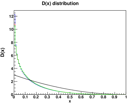
Figure 3.1 shows various solutions $D(T,x)$ of the evolution equation. The blue curve represents the solution accurate up to LO. The red curve shows the distribution for the generation with decreased time limit, while the green one shows the one obtained by adding the $\Delta$-correction directly to the kernel using eq. (3.2). The black curve representing the initial distribution $D(t_{0},x_{0})$ is also shown.

It is clearly seen that red and green curves coincide, which confirms the statement of Curci–Furmanski–Petronzio: decreasing the time limit has the same effect as correcting the kernel with the $\Delta$-function.

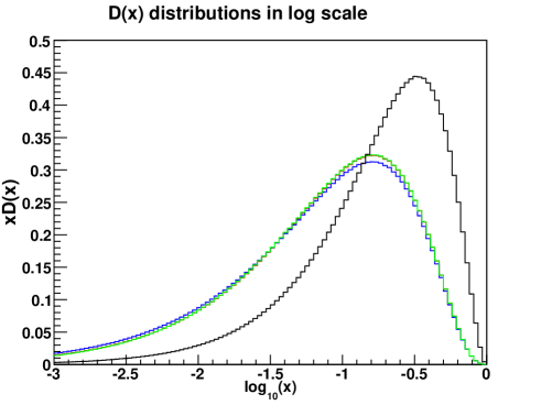
The differences between various curves are better visible in Figure 3.2, which shows the same distributions multiplied by $x$ and plotted as a function of $log_{10}\;x$.

Figure 3.3: Ratios of $D(x)$ distributions: (b) divided by (a) (red), (c) divided (a) (green) and (b) divided by (c) (blue). The notation (a), (b) and (c) and parameters are the same as in Figure 3.1

.

Figure 3.4: Ratios of $xD(x)$ distributions as functions of $log_{10}x$. The parameters and the meaning of colors are the same as in Figure 3.3

.

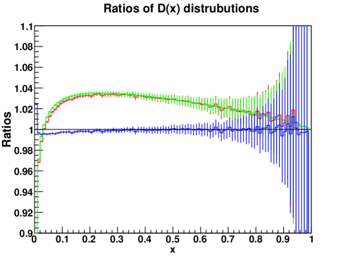
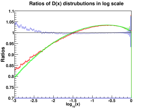
In order to see even better the differences between various resulting distribution we plot in Figures 3.3 and 3.4 the ratios of the same distributions, once again as functions of $x$ and $log_{10}\;x$. Now, the red curve represents the ratio of the solution obtained by decreasing time limit and the one accurate up to the LO level. The green curve shows the ratio of the solution obtained by using the direct $\Delta$-correction to the kernel and the one obtained by using the LO approximation. Finally, the blue curve represents the ratio of the distribution obtained by decreasing the time limit and the one with the direct $\Delta$-correction to the kernel. It is seen that the last ratio is close to one. Once more it indicates clearly our basic result that shifting the evolution time limit by $\ln z$ (factorization scale by factor $z$) gives the same result as using the direct $\Delta$-correction to the kernel in the way described by Curci–Furmanski–Petronzio [2].

We have checked that the slight systematic difference between red and green curve in Figures 3.3 and 3.4 for small $x$ values results from the fact that in the MC implementation shortening $T\to T+\ln(1/z_{i})$ below the initial $t=0$ cannot be realized. Also, one has to keep in mind, that such a shortening evolution time limit induces not only ${\cal O}(\alpha_{s})$ contribution to the evolution kernel, but also ${\cal O}(\alpha_{s}^{2})$ term, which is not taken into account in the present study. Due to smallness of $\alpha_{s}$ the corresponding effect seems to be negligible.

Let us finally mention that all plots and histograms presented in this sections have been obtained using Monte Carlo software environment MCdevelop [9] and ROOT [10] package.

4 Summary

The most important result presented here is checking the equivalence of two methods of implementing the $\Delta$-function of CFP in the Monte Carlo environment. In the first method the evolution time range was made shorter, step by step, after each iteration. In the second method, the evolution time limit was kept fixed, but the $\Delta$-function was added directly to the LO evolution kernel as NLO correction, by means of correcting generated events with the help of a relevant MC weight. Both methods have given the same results, within the statistical error of the MC computations. The small systematic difference between the results of both methods is the region of small $x$ values is well understood.

References

- [1] G. Altarelli, R. K. Ellis, and G. Martinelli, Nucl. Phys. B157 (1979) 461.
- [2] G. Curci, W. Furmanski, and R. Petronzio, Nucl. Phys. B175 (1980) 27.
-
[3]
M. Ciafaloni, Nucl. Phys. B296 (1988) 49;
S. Catani, F. Fiorani and G. Marchesini, Phys. Lett. B234 339, Nucl. Phys. B336 (1990) 18;
G. Marchesini, Nucl. Phys. B445 (1995) 49. - [4] S. Jadach, A. Kusina, M. Skrzypek, and M. Slawinska, Nucl. Phys. Proc. Suppl. 205-206 (2010) 295–300, 1007.2437.
[5]
L.N. Lipatov, Sov. J. Nucl. Phys. 20 (1975) 95;
V.N. Gribov and L.N. Lipatov, Sov. J. Nucl. Phys. 15 (1972) 438;
G. Altarelli and G. Parisi, Nucl. Phys. 126 (1977) 298;
Yu. L. Dokshitzer, Sov. Phys. JETP 46 (1977) 64. - [6] R. Ellis, W. Stirling, and B. Webber, QCD and Collider Physics. Cambridge University Press, 1996.
[7]
D. J. Gross and F. Wilczek, Phys. Rev. Lett. 30 (1973) 1343;
H. D. Politzer, Phys. Rev. Lett. 30 (1973) 1346;
D. J. Gross and F. Wilczek, Phys. Rev. D8 (1973) 3633;
H. D. Politzer, Phys. Rep. 14 (1974) 129. - [8] K. Golec-Biernat, S. Jadach, W. Płaczek, and M. Skrzypek, Acta Phys. Polon. B37 (2006) 1785–1832, hep-ph/0603031.
- [9] M. Slawinska and S. Jadach, Comput. Phys. Commun. 182 (2011) 748–762, 1006.5633.
- [10] R. Brun and F. Rademakers, Nucl. Instrum. Meth. A389 (1997) 81–86.