Implementing a search for aligned-spin neutron star - black hole systems with advanced ground based gravitational wave detectors
Abstract
We study the effect of spins on searches for gravitational waves from compact binary coalescences in realistic simulated early advanced LIGO data. We construct a detection pipeline including matched filtering, signal-based vetoes, a coincidence test between different detectors, and an estimate of the rate of background events. We restrict attention to neutron star–black hole (NS-BH) binary systems, and we compare a search using non-spinning templates to one using templates that include spins aligned with the orbital angular momentum. To run the searches we implement the binary inspiral matched-filter computation in PyCBC, a new software toolkit for gravitational-wave data analysis. We find that the inclusion of aligned-spin effects significantly increases the astrophysical reach of the search. Considering astrophysical NS-BH systems with non-precessing black hole spins, for dimensionless spin components along the orbital angular momentum uniformly distributed in , the sensitive volume of the search with aligned-spin templates is increased by compared to the non-spinning search; for signals with aligned spins uniformly distributed in the range , the increase in sensitive volume is a factor of .
I Introduction
We present here the first realistic gravitational wave (GW) search pipeline for coalescing compact binaries containing a neutron star (NS) and a black hole (BH) with spin aligned with the orbital angular momentum. Our pipeline includes a physical template bank, signal-based vetoes and coincidence between multiple detectors. We show that a simple extension of traditional search methods to include the effects of aligned spin can lead to an appreciable improvement in detection efficiency, even during the early observational runs of advanced GW detectors, before they reach full sensitivity. See Harry (2010); Accadia et al. (2012) for descriptions of the advanced LIGO and Virgo detectors. In addition, the KAGRA detector is currently under construction in Japan Somiya (2012) and an advanced detector has also been proposed in India Iyer et al. (2011).
In this paper we shall focus on neutron star–black hole (NS-BH) binary systems which are promising sources for the advanced detectors and pose a computational challenge. Based on our current understanding of the population and evolution of binary systems, it is expected that the coalescence rate for NS-BH systems within the sensitive volume of the advanced detectors is in the range 0.2-300/year Abadie et al. (2010a). To achieve this detection rate, we must be able to distinguish signals from noise at a matched filter signal-to-noise ratio (SNR) of or above in the LIGO detectors. Thus we require accurate models of the signal waveforms for matched filtering, as well as effective methods to exclude false alarms due to non-Gaussian artifacts in the data.
With one exception Abbott et al. (2008), previous searches of initial LIGO data did not incorporate the effect of the compact objects’ angular momentum (spin) in the waveforms used for filtering the data111However, some other LIGO searches (see e.g. Aasi et al. (2013a)) have quantified how well they could detect spinning systems, even though they conducted the primary search using waveform models without spin.. This was because the search methods and detector sensitivity at the time did not warrant the inclusion of spin effects Abbott et al. (2008); Van Den Broeck et al. (2009). In general, including extra parameters such as spin in the search increases the size of the template bank, making the search computationally more demanding and increasing the false-alarm rate. An important question therefore is whether more accurate waveform models can offset this increase in false-alarm rate. It has been recently demonstrated that, for the case of BH-BH binaries, including a single effective aligned-spin parameter in the search space does improve the detection rate Privitera et al. (2014), but the question remains open for NS-BH systems. The initial LIGO detectors had relatively low sensitivity at higher frequencies meaning that the modified phase in the expected signal due to spin was less visible. The situation will be different in the advanced detector era. The advanced LIGO detectors will be able to discern the extra features in the waveform due to the effects of spin for a significant number of events Brown et al. (2012); Harry et al. (2013). Furthermore, the increased computational requirements for spinning searches can be met by improving the analysis software used to process the data and exploiting modern computational platforms such as graphics processing units.
The aim of this paper is twofold. First, we show that it is indeed important to incorporate spin in searches for NS-BH compact binary coalescence (CBC) events, even in the early advanced detector era. Second, we describe a new software package for CBC searches known as PyCBC, which is designed to meet the computational challenges of the advanced detector era.
Since the NS-BH merger rate is uncertain by about three orders of magnitude, it is clear that much remains unknown about the population of compact binary systems. A measurement of this rate would constrain models of the formation and evolution of stellar binaries Mandel and O’Shaughnessy (2010); O’Shaughnessy et al. (2005). NS-BH systems are also of interest astrophysically because they (along with double NS systems) are expected to be progenitors of short-hard gamma-ray bursts Eichler et al. (1989); Narayan et al. (1992). A detection of NS-BH coalescences would allow us to explore the behavior of compact objects in the strong field regime and observation of the merger phase would provide important information about the tidal disruption of NS and their equation of state Ferrari et al. (2010); Pannarale et al. (2011). NS-BH systems have thus been of significant interest for numerical relativity simulations Etienne et al. (2008, 2009); Duez et al. (2008); Shibata and Uryū (2006); Löffler et al. (2006).
The spin angular momentum of binary objects affects the intrinsic evolution of their orbits due to spin-orbit and spin-spin couplings in the post-Newtonian orbital energy and GW flux. If the spin of the objects in the binary system is not aligned with the orbital angular momentum, then the orbits will also precess Apostolatos et al. (1994). Searches for such precessing signals are computationally demanding as such signals are described by many independent parameters. Previous investigations of the effect of spin on GW searches largely focused on the precessing case, for which a number of phenomenological search templates have been proposed Apostolatos (1995, 1996); Buonanno et al. (2003); Grandclement et al. (2003). However, none of these attempts were successful when applied to real data. Here we focus instead on the simpler problem of “aligned-spin” systems, where the spin angular momenta are aligned with the orbital angular momentum.
Including the effect of aligned spins still increases the size of the template bank. The larger number of templates increases the number of false alarms in pure noise. False alarms from non-Gaussian transients (glitches) triggering spinning templates had an adverse affect on previous attempts to include spin effects in searches Van Den Broeck et al. (2009). To counter this problem we also include here a signal-based veto, the -test Allen (2005); Babak et al. (2013) used in previous LIGO searches Abbott et al. (2009a); Aasi et al. (2013a); Abadie et al. (2012a, 2011, 2010b); Abbott et al. (2009b, 2006, 2004, 2005a, 2005b); Abadie et al. (2010c). This veto reduces the significance of glitch-induced triggers in the search, and thus greatly reduces the threshold on signal SNR that must be applied to achieve a desired false-alarm rate. In order to simulate the behavior of real advanced LIGO data, we analyze two months of real data from the two 4 km initial LIGO detectors at Hanford (H1) and Livingston (L1), recolored to a spectrum typical of the sensitivity that advanced detectors are expected to achieve in 2016-2017 Aasi et al. (2013b).
A comparison of searches with and without including spin effects depends critically on the expected distribution of spin magnitudes and orientations in the target astrophysical population. The maximum theoretical spin for an isolated Kerr BH is given by where is the dimensionless ratio between the spin angular momentum and the mass . The maximum value of to which a BH can spin up due to accretion of matter from a thin accretion disk is thought to be very close to this limit Thorne (1974). A number of stellar mass BHs have been discovered using X-ray techniques. Observations suggest that many of them have quite large spins, even close to this maximum limit McClintock et al. (2013). This is especially true of the BHs in high-mass X-ray binaries whose measured spins are all above . These high-mass systems are the most likely to form NS-BH binaries and it is likely that the BHs were born with these high spins since they have had insufficient time to spin up due to accretion McClintock et al. (2013).
Binary systems that are potential sources for advanced LIGO are expected to have undergone a hypercritical common envelope (HCE) phase Dominik et al. (2012). The available modeling of this phase suggests that hypercritical accretion onto the BH will further spin up the BHs O’Shaughnessy et al. (2005) from their spin values before HCE. Taken in conjunction with the X-ray data, this suggests that many of the BHs observable to the LIGO detectors will have large spins. We test our analysis with the full range of spin values from to (where negative values indicate spins anti-aligned with the orbital angular momentum) but we also display results for restricted ranges, including a high spin range to .
The maximum possible spin for a NS is set by the break-up velocity, which for expected equations of state corresponds to Lo and Lin (2011); realistic NS values are thought to lie below this, braked by r-mode instabilities and perhaps by GW emission Wagoner (1984); Bildsten (1998); Chakrabarty et al. (2003). The maximal spin observed for accreting millisecond pulsars corresponds to , but the maximum value observed in a binary of two compact objects is only Damour et al. (2012). In NS-BH binary systems the BH is likely to form first due to its larger mass and is therefore unable to contribute matter to spin up the NS. We therefore largely ignore the spin of the NS in NS-BH binaries and concentrate on a single spin, that of the BH.
While some studies suggest that an appreciable fraction of NS-BH systems may have significant spin misalignments Belczynski et al. (2007), others suggest a small misalignment for most systems Kalogera (2000). For small misalignments, the aligned-spin search would be close to optimal. A closed form for the waveform of a single spin precessing system has recently been provided Lundgren and O’Shaughnessy (2013), but a full search based on this method has not yet been implemented and may, as an initial step, require an efficient single-spin aligned search similar to that presented here. We may therefore view this investigation as the first step towards a fully precessing search.
A complete gravitational waveform includes the merger and post-merger ringdown signal as well as the inspiral signal. For simplicity, we ignore the merger and ringdown part of the waveform and ignore the possibility that the NS may be tidally disrupted and destroyed during the inspiral phase Foucart et al. (2013). A particular recent model for a complete waveform is EOBNRv2, based on the Effective One-Body (EOB) framework calibrated by numerical relativity waveforms Pan et al. (2011). Standard inspiral-only waveforms were found to match EOBNRv2 waveforms for total masses below 11.4 solar masses for the advanced LIGO detectors Brown et al. (2013). Most of our simulated signals have total masses below this limit, although it is not yet known what the effect of spin is on this limit. The effect of merger and ringdown will be studied in detail elsewhere.
The aligned-spin search pipeline employed in this paper is based on the PyCBC software package pyc (a). PyCBC is a newly-developed toolkit for CBC searches in the advanced detector era written in the Python programming language. It is based on modular software libraries: modules in isolation are quite simple, but can be put together in useful and sophisticated ways. PyCBC allows scientists to create complicated entire end-to-end pipelines for performing CBC searches. PyCBC also enables scientists to use GPUs in a transparent manner. PyCBC builds on software from the LIGO Algorithms Library LAL used in previous LIGO searches.
The rest of this paper is organized as follows. Sec. II introduces our search pipeline. Sec. III introduces the PyCBC toolkit and the computational details of the pipeline; this section can be read independently. The template banks are described in Sec. IV and further details of the search are in Sec. V. Sec. VI presents the main results and Sec. VII provides a summary and directions for future work.
II Search method
A fair comparison of the effects of spin in a search needs to take into account all the details of a search of real GW data. Therefore we implement a prototype pipeline which can search for both spinning and non-spinning systems. This prototype pipeline is applied to a synthetic data set obtained by recoloring initial LIGO data as described in Aasi et al. (2014).
We first summarize the basic matched-filtering method employed, which is described in more detail in Allen et al. (2012). Let be the data stream from a GW detector. Let be the noise and a GW signal which may or may not be present in the data stream. Thus, in the absence of a signal, and otherwise. We denote the Fourier transform of a time series as defined as
| (1) |
With the assumption that is a stationary noise process, we define its single-sided power spectral density (PSD) as
| (2) |
where denotes the expectation value over an ensemble of noise realizations. While the assumption of stationarity is not a good one for realistic data, this definition of the PSD is still applicable over short time scales. The non-stationarity is handled by continuously estimating from the data using a modification of the Welch method Percival and Walden (1993) as described in Allen et al. (2012).
The signal as seen in the detector is a linear combination of the two polarizations and :
| (3) | |||||
Here the beam pattern functions depend on the sky position given by a unit-vector pointing towards the source, and on the polarization angle (see e.g. Apostolatos et al. (1994)). The beam pattern functions can be taken to be constant for the duration that the signal is seen by the detector. is a suitably defined arrival time: in this case we will use an inspiral waveform described by the post-Newtonian approximation, then a convenient choice for is the termination time, such that the frequency of a signal with GW phase evolution formally becomes infinite at . is the corresponding termination phase. In the restricted post-Newtonian approximation, the slowly varying amplitude is given by
| (4) |
with being the chirp mass of the binary, the total mass, the symmetric mass ratio, the effective distance, the angle between the line of sight from the binary system to Earth and the orbital angular momentum, and the distance to the binary system (see e.g. Allen et al. (2012)).
The termination time can be searched over by an inverse fast Fourier transform (FFT) and the search over can be handled by an analytic maximization. As shown in Allen et al. (2012), this results in having to compute the complex statistic
| (5) |
where is a suitably normalized inspiral waveform template expressed in the frequency domain. The SNR is then defined as where
| (6) |
With this normalization, in Gaussian noise in the absence of a signal we would have . For practical purposes the integrations in (5) and (6) are limited to a lower frequency cutoff below which the detector is dominated by seismic noise and an upper frequency cutoff beyond which the post-Newtonian waveform becomes unreliable.
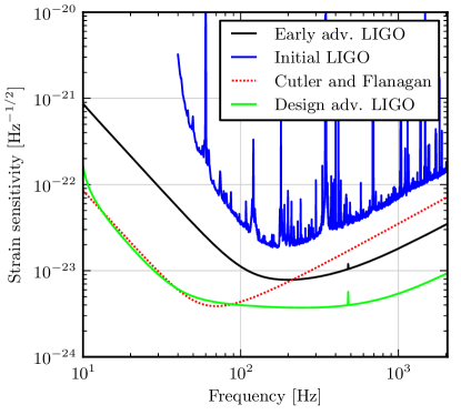
This work focuses on a sensitivity curve that could reasonably represent the early (2016) runs of advanced LIGO Aasi et al. (2013b) and uses a lower frequency cutoff Hz. However, in Sec. IV we also investigate three different sensitivities, namely: i) the typical sensitivity of initial LIGO during its sixth scientific run Abadie et al. (2012b) with Hz; ii) the projected sensitivity from Cutler and Flanagan (1994), used for ease of comparison with the results of Apostolatos (1996), with Hz; and iii) the zero-detuned, high-power design sensitivity of the mature advanced LIGO detectors Aasi et al. (2013b) with Hz. These curves are shown in Fig. 1.
The SNR works well as a detection statistic in Gaussian noise. To deal with non-Gaussian noise of realistic detectors and veto non-Gaussian transients of non-astrophysical origin, other statistics have been developed. A widely used signal-based veto is the reduced -statistic Allen (2005), which computes the partial SNRs in non-overlapping frequency bands and combines them as
| (7) |
The bands are chosen so that a true signal with total SNR would have a partial SNR of in each band; the union of the bands must cover the full frequency range used to compute . We note that computing for each time sample requires inverse FFTs and is thus computationally expensive. The exact computational method of calculating and given a discretely sampled time series , the FindChirp algorithm, is described in Allen et al. (2012). We continue to use the same algorithm in this work.
In order to mitigate the effect of non-Gaussian transients that plagued previous spinning studies Van Den Broeck et al. (2009) we use a modified detection statistic that extends the usual SNR using the -veto, known as the re-weighted SNR statistic Abadie et al. (2012a); Babak et al. (2013):
| (8) |
We threshold on both the SNR and re-weighted SNR when generating candidate events, and rank them via re-weighted SNR; this choice was found to be sufficient for our purposes, although it is possible that other choices of ranking statistic would perform even better.
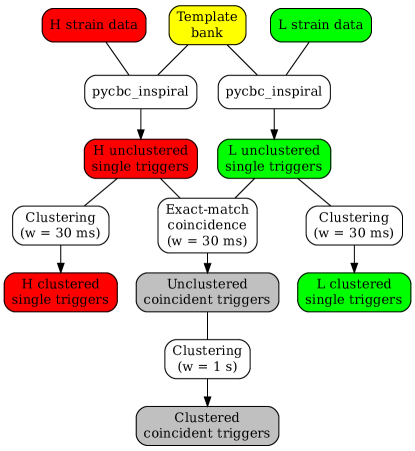
Our prototype search pipeline is sketched in Fig. 2. We choose “standard” values for most parameters in the pipeline (such as the number of bands , the coincidence windows etc.) that have been commonly used in other searches Babak et al. (2013). Notable differences are the coincidence method, and the use of a template bank which is common for all detectors and fixed for the whole data set. A more detailed tuning of the pipeline could improve the sensitivity further. The next sections introduce the PyCBC toolkit and describe the main components of the pipeline in detail.
III The PyCBC Toolkit
Since 2004, when the first result of a CBC search on LIGO data was published, the bulk of the data analysis for CBC searches has been carried out using software from the LIGO Algorithms Library (LAL) LAL . This is a set of tools and applications written in the C programming language. The computational landscape has diversified significantly over the last 10 years. In particular, the use of GPUs for general purpose computing is now more widespread and even central processing unit (CPU) design is moving towards parallel architectures. It is important that the software infrastructure for GW searches is flexible enough to keep up with this diversity.
As we saw in the previous section, the computational cost for CBC analyses is typically dominated by the cost of performing Fourier transforms, primarily in computing the SNR and the statistics, described earlier, for each inspiral waveform in a large template bank. One strategy would then be to move the FFT calculations to GPUs and keep the remaining computations on the usual CPU of a computer. This would require relatively minor modifications to the existing software in LAL and we could continue using LAL without major modifications. While this does speed up the analysis time somewhat, a detailed profiling of the code reveals that the GPUs are very under-utilized and significant time is spent in data transfers between the CPU and the GPU. This suggests that further development should allow the majority of the computation to run on the GPU.
In this section we describe a new toolkit, PyCBC pyc (a), which builds on the tools available within LAL and makes it easier to assemble complex end-to-end pipelines, and also enables the use of GPUs in a transparent and user-friendly manner. PyCBC is written in the Python programming language pyt , a convenient high-level scripting language with a large user community. There are extensive collections of external libraries in Python for a wide variety of tasks, including interfaces to GPUs and general purpose scientific computing. The Python modules of PyCBC need to be able to access the existing LAL software written in C. This is important firstly because C can often be computationally more efficient and secondly because LAL has an extensive collection of GW-specific functionality which has been well tested and widely used within the LIGO and Virgo collaborations.
PyCBC uses the SWIG framework swi to access LAL software for CPU computations. This enables one to perform computations within PyCBC without sacrificing computational speed. PyCBC supports GPU computation via either the CUDA cud or OpenCL ope architectures, using respectively the PyCUDA pyc (b) or PyOpenCL packages pyo .
An example will help us illustrate how these design choices lead to a toolkit that is flexible and maintainable, easy for users to code in, and transparently provides the performance capability of GPUs, while also allowing the same code to run optimally on a CPU when that platform is chosen instead. A simplified script for the basic matched-filtering operation that performs the convolution of a template with a data segment in PyCBC is as follows:
While a real code is somewhat more complex, particularly due to the thresholding, clustering, and vetoes mentioned earlier, the above sample code shows how the design of PyCBC achieves several important goals:
-
1.
Transferring data between the CPU and GPU is transparent to the author of the scripts: he or she need only perform the relevant calculations inside the with CUDAScheme block (a context block in Python) and memory will automatically be transferred as it is used in computations within the block. In actual scripts, the context (in the example above, CUDAScheme) is a variable determined at run-time, so that the same script may execute on any CPU, CUDA, or OpenCL platforms.
-
2.
We leverage Python’s object oriented capabilities to “make simple things simple.” In the example above, the multiplication of the template by the data requires only the single operator, though in reality it represents an element-by-element multiplication of two frequency series, which is also transparently sanity-checked first to ensure the two series have the same length and frequency resolution.
-
3.
Simplicity for the user is mirrored by comparative simplicity for PyCBC developers, because the basic PyCBC objects (vectors, time-series, and frequency-series) leverage the uniform interface for arithmetic and basic mathematical operations presented by Numpy (used for CPU), PyCUDA, and PyOpenCL. Considering the wide variety of basic operations, many of which can have multiple instances depending on the precision and type (real or complex) of their inputs, this is a huge saving in development overhead, and immediately provides a functionality not present in LAL.
-
4.
The inverse FFT is transparently dispatched to the appropriate library (CUFFT cuf for CUDA, FFTW Frigo and Johnson (2005) or MKL mkl for CPU) which again is not written by the PyCBC developers. In the end, very little code must be separately written for the three supported platforms; in the example listing above, only the generation of the frequency domain waveform would be written and maintained by the PyCBC project directly.
As a result of this design, it is also simple to change which parts of the computation are performed on the CPU, and which on the GPU. The code listing above shows part of a script where the entire matched filter computation, and not only the inverse FFT, is performed on the GPU. It therefore makes more efficient use of the GPU while at the same time requiring very little additional coding.
Given the large number of templates in the spinning template bank, our search is computationally costly; the vast majority of the cost is represented by the matched-filtering stage, while coincidence and clustering are comparatively trivial. The Atlas cluster atl at the Albert Einstein Institute in Hannover is equipped with Nvidia Tesla C2050 GPUs and PyCBC’s flexibility allows us to accelerate the search by running the matched-filter stage on these GPUs. Our implementation of the CBC matched filtering engine uses roughly 35% of the GPU time as reported by the nvidia-smi tool nvi . A detailed profiling of the code, a performance comparison between CPUs and GPUs, and further optimizations will be presented elsewhere.
IV Template banks
To describe the template bank used in our search, we establish some standard notation. The inner product between two signals and , also known as the overlap, is defined as
| (9) |
We define the normalized signal as . The match between the two waveforms is defined by maximizing the inner product between the two normalized waveforms over the time of arrival and the phase of, say, :
| (10) |
Consider a template bank of waveforms with that is meant to cover a particular parameter space of masses and spins. The fitting factor for any waveform in the parameter space with the template bank is defined as:
| (11) |
In constructing a template bank, a common requirement is that any waveform in the target parameter space must have a fitting factor larger than 0.97 Babak et al. (2013); thus, any waveform in the parameter space must match some waveform in the template bank by at least 0.97. In the actual spinning template bank employed we find that matches can fall as low as . This small deterioration of the minimal match condition occurs only in a small region of parameter space for low values of and will not greatly affect signals with BH masses below and NS masses around . The cause of these lower match values is discussed towards the end of this section.
In this section we compare a spinning template bank with a non-spinning template bank. Both banks are constructed using a stochastic placement procedure that was previously presented in Brown et al. (2012); a general introduction to stochastic template banks can be found in Harry et al. (2009); Babak (2008). We use the stochastic bank algorithm implemented within the PyCBC framework. The template waveforms use the restricted frequency-domain TaylorF2 approximant containing 3.5 pN non-spinning phase corrections Blanchet et al. (1995, 2004) and 2.5 pN spinning phase corrections Arun et al. (2009); Cutler and Flanagan (1994); Kidder (1995); Blanchet et al. (2006). When calculating the matched-filter SNR, our template waveforms terminate at a frequency corresponding to the innermost stable circular orbit (ISCO) of a Schwarzschild BH of the same total mass as the template, i.e. . This was the standard choice in past CBC searches. However, in the construction of our banks, templates are assumed to terminate at a fixed frequency of 1000 Hz, which is close to the maximum ISCO frequency in our parameter space. Past searches also made a fixed-frequency assumption. Although PyCBC has the ability to construct banks with a varying termination frequency, we do not explore the effect of this choice in this study.
The template bank for the non-spinning search has a BH mass ranging from 3 to 15 and a NS mass ranging from 1 to the equal-mass boundary . We also impose the constraint . Both spins are constrained to zero. This results in templates. The bank for the spinning search is constructed instead with , , and . Such settings produce templates, which turn out to be mostly clumped around extremal values of .
Fig. 3 shows the mass boundary of the two banks. As can be seen, the non-spinning bank has a larger mass range for the NS than the spinning bank, in particular it includes part of the binary BH region. We make this choice partly because this is how a traditional low-mass non-spinning search would be carried out and partly to allow spinning signals to be recovered by non-spinning templates with similar chirp mass but closer to the equal-mass boundary, thanks to a degeneracy between spin and symmetric mass ratio Baird et al. (2013). In other words, we explicitly favor the non-spinning search by tolerating a bias in the recovered symmetric mass ratio. The fraction of templates in the non-spinning bank with is .
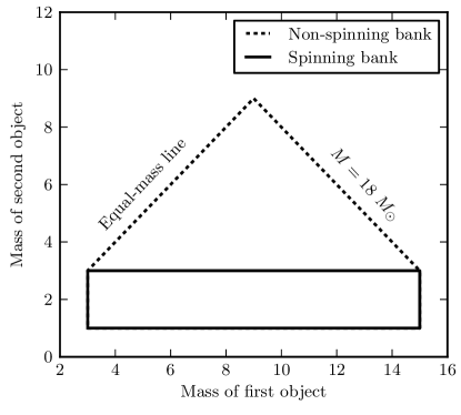
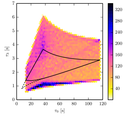
Fig. 4 shows the template density of the spinning bank in the plane, where
| (12) | |||||
| (13) | |||||
are the chirp times Sengupta et al. (2003) extended to include spin-orbit effects, and Hz is a fiducial frequency. The non-spinning part of the NS-BH parameter space is shown as a black contour in the figure and the region covered by the non-spinning bank corresponds to the black contour plus the small area delimited by the dashed contour. As can be seen, including the effect of spin broadens the covered region significantly. Moreover, although the density remains approximately constant inside the black contour, it increases noticeably outside; in particular, a large amount of templates is concentrated at small values. Better coordinates for representing spinning templates in which the template density is nearly constant are given in Brown et al. (2012); Ohme et al. (2013).
IV.1 Fitting-factor calculations
The behavior of a template bank with respect to various signals can be studied without the effect of detector noise by numerically evaluating the fitting factors defined in (11), which can be done by PyCBC. In order to get a first characterization of the effect of spin on a few non-spinning banks associated with the different sensitivity curves and lower-frequency cutoffs shown in Fig.1, we calculate the fitting factors for such banks using simulated signals with fixed masses ( and ) and a full range of physical spins for the heavier object () and zero spin for the lighter object (). The signals are simulated using the standard time-domain SpinTaylorT2 approximant available in LALSimulation LAL . In principle one could choose other approximants such as SpinTaylorT1 or SpinTaylorT4, which treat the Taylor expansions of the energy and flux differently. However, we choose SpinTaylorT2 because it is essentially the time-domain version of our frequency-domain templates, reducing issues related to agreement between signal and template approximants which are outside the scope of this paper. The waveform generation starts at 20 Hz (well outside the integration range of the matched filter) and terminates at the minimum-energy circular orbit (MECO) after which the evolution of the orbit is no longer expected to be adiabatic (see e.g. Pan et al. (2004)). This choice is different from the termination condition assumed in the construction of the template banks (1000 Hz) as well as the upper frequency limit used in matched filtering (the template ISCO frequency). In reality, a physical NS-BH waveform terminates with the merger and ringdown, typically at frequencies higher than ISCO, so any choice of abrupt termination of the signal is artificial. Given that we do not consider NS-BH merger and ringdown in this study, MECO is a good choice both for implementation reasons and because it is also almost always greater than ISCO. Nevertheless, as discussed later in this section, this discrepancy can affect the fitting factor of binaries at high mass or high positive BH spin. The performance of our template banks for more realistic signal models including merger and ringdown will be assessed in a future study.
The results for the different non-spinning banks are given in Fig. 5, showing similar behavior over different sensitivity curves and lower frequency cutoffs.
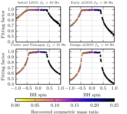
As can be seen, in all banks there is a range of low BH spins for which the non-spinning bank is able to match the spinning signals fairly well, but then a sharp fall-off in the fitting factor occurs above . The shading (color online) of the points shows the recovered value of in the non-spinning bank. Although the signals are simulated with , as the spin is increased the recovered value of also increases, compensating for the larger spin. It can be seen that the sharp fall-off in the fitting factor for positively aligned systems is associated with the maximum physical value of , corresponding to equal mass templates. Thus, if we had injected signals with a different value of , the fall-off in match could happen at different values of . For the equal mass case , for instance, we are already at the boundary and cannot increase any further to compensate for the spin. The match then starts to decrease sharply even for small positive spins. In the rest of the paper we will only consider the early advanced LIGO sensitivity curve (top-right panel of Fig. 5) and references to “the (non-)spinning bank” will denote banks built for this case.
The loss of match at high BH spins can be further understood by comparing the true and recovered values of the masses in the non-spinning bank, as is done in Fig. 6.
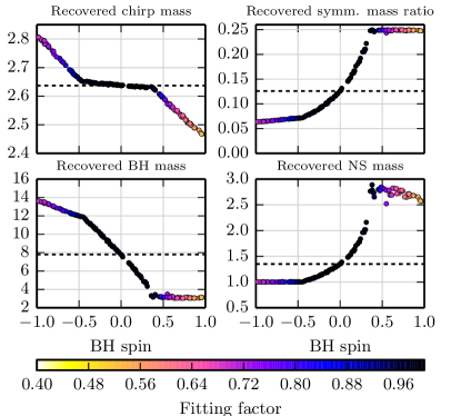
The shading now shows the match and again it is clear that the rapid fall-off in match for the positively aligned waveforms is due to the boundary at . The rapid fall-off in the match for anti-aligned waveforms is due to a different effect, namely the fact that the minimum in all template banks is 1 . Unlike the case, this is not a physical boundary and one could obtain better matches for highly spinning anti-aligned systems by lowering the minimum NS mass in the template bank.
The recovered mass and spin parameters in the spinning bank are given in Fig. 7.
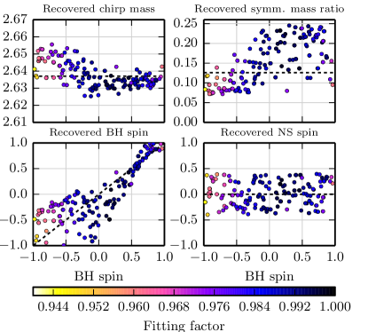
Here, as expected the templates are all well-matched, although there is a slight bias in the recovered masses and values. The recovered value is seen to be widely scattered and it is clear that this does not have any significant impact on the match, nor is its value well recovered by the bank. In other aligned-spin search investigations Privitera et al. (2014) a single effective spin parameter was used and the minimal impact of the value seen here is consistent with that approach. The fact that the matches descend below despite the design choice that the bank should have a minimal match of was also noted in Harry et al. (2013) and was explained there by an inconsistency between the termination condition of template and signal waveforms.
As an overall test of the performance of the two banks over the NS-BH parameter space, we calculate fitting factors with SpinTaylorT2 signals uniformly distributed across the parameter space. The result is shown in Fig. 8,
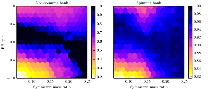
illustrating the deficiency of the non-spinning bank over the parameter space. It can be clearly seen that the values of at which the match suddenly drops are a function of ; for equal-mass systems the match starts to drop for . Interestingly, the spinning bank can have a mismatch as large as 15% in some parts of the parameter space. As noted already, this is likely an effect of the different (mass- and spin-dependent) termination conditions of the template and test waveforms. In fact, a template terminating before the signal loses the signal power contained between ISCO and MECO, while in the case of a template terminating after MECO the SNR normalization defined in Eq. 6 is too large; both cases result in an effective SNR loss. This hypothesis is supported by the fact that most of the residual mismatch on the right plot of Fig. 8 covers the region of plane where a large difference exists between the MECO frequency and either the fixed termination at 1000 Hz assumed in constructing the bank or the ISCO termination used for the template matched filtering.
Although our test signals and templates both use spinning phase corrections up to 2.5 pN order, 3.5 pN corrections have been implemented during the development of this paper and are now ready to be used in searches Marsat et al. (2013); Wade et al. (2013). Unfortunately, including 3.5 pN spinning terms in the MECO definition can lead to very different termination frequencies for our SpinTaylorT2 signals, introducing technical difficulties which complicate our fitting factor calculation. Nevertheless, as a rough characterization of the effect of 3.5 pN terms, we test our non-spinning, 2.5 pN TaylorF2 bank against ISCO-terminated TaylorF2 signals with 2.5 pN and 3.5 pN spinning terms. We find that the largest variation in fitting factor when going from 2.5 to 3.5 pN signals is , which is comparable to the maximum mismatch used for constructing the bank and well below the loss due to neglecting spinning terms altogether. A more detailed characterization of the inclusion of 3.5 pN spin terms represents a separate study, but we see no reason for not using the best available phasing in future searches.
V Details of the pipeline
After having described the template banks, the next step is evaluating the performance of a full search pipeline running on realistic data. This section describes in detail the various components of the pipeline that we implement (see Fig. 2) and the corresponding parameter choices.
V.1 Inspiral trigger generation
Strain data are first processed by a PyCBC implementation of the standard FindChirp algorithm Allen et al. (2012) used in previous CBC searches. After conditioning the data Babak et al. (2013) and estimating the noise PSD, the SNR time series is computed for each template with a low-frequency cutoff of 30 Hz. This is lower than past searches because we are targeting the early advanced-LIGO sensitivity. Local maxima of the SNR time series that satisfy the condition are identified. The -statistic is then computed for each surviving maximum via (7) using 16 frequency bands, as is typical in CBC searches Abbott et al. (2009a); Aasi et al. (2013a); Abadie et al. (2012a, 2011, 2010b); Abbott et al. (2009b, 2006, 2004, 2005a, 2005b); Abadie et al. (2010c), and combined with the SNR via (8) to obtain . In order to reduce the very large number of maxima produced by glitches, only those with are kept as candidate triggers. Such triggers are then stored in a MongoDB database mon , where they can be conveniently accessed by the next processing stages and also queried to investigate the features of the data and the search.
The thresholds on SNR and re-weighted SNR used here are higher than past CBC searches (e.g. Abbott et al. (2009b); Abadie et al. (2010b, 2011, 2012a); Babak et al. (2013)) as they are chosen to fit the triggers into the available database storage space, which is limited in our prototype setup. There is, in principle, no technical barrier to extending the storage space of the database to handle a larger number of events, which would allow one to lower the threshold back to the usual value.
Even if the noise PSD is continuously estimated from the data in order to evaluate the SNR, our template banks are constructed using the early advanced-LIGO model PSD and thus are constant for the whole data set. This is also a notable difference with past searches, where template banks were regenerated on a time scale of 30 minutes to account for the variability of the noise PSD. Our choice is based on simplicity and the relatively high computational cost of template bank generation. It is also partly justified by the fact that the synthetic data we analyze is recolored to the same noise curve used for constructing the banks. Although the impact of a fixed or varying bank on the sensitivity of a search is not yet fully understood, we expect our choice to have a small effect on the result of our comparison.
V.2 Coincidence and clustering
The next stage of the pipeline is the identification of triggers in coincidence between the Hanford and Livingston detectors. Although the recolored strain data we analyze covers a two-month period, the different duty cycles of the detectors reduce the amount of data analyzed in coincidence to about 25 days.
Because we store the triggers in a centralized database, different coincidence methods can be applied to them. We choose an exact-match method, where a trigger in detector A can only form a coincidence with a trigger in detector B if the two triggers share the same template, similar to Privitera et al. (2014). This method has the advantage of simplicity and is straightforwardly applicable to parameter spaces of any dimensionality. It requires however a common template bank for all detectors, another difference with respect to past CBC searches, as discussed above. A systematic comparison of different coincidence methods is outside the scope of this paper. Considering that the maximum arrival time delay between Hanford and Livingston is ms, and that the uncertainty in coalescence time is of the order of a few milliseconds Nielsen (2013), we choose a conservative coincidence window of ms. Each pair of coincident triggers is stored in the database and is tagged with the combined SNR and re-weighted SNR, defined respectively by summing in quadrature the single-detector SNRs and re-weighted SNRs.
In order to keep only the most representative trigger among all the triggers produced by a single inspiral signal or glitch, a final clustering step is performed on coincident triggers. A trigger is defined as representative if no other triggers with higher combined re-weighted SNR exist within s.
Finally, in order to study the distribution of single-detector false alarms, we also perform clustering of single-detector triggers. This works in the same way as coincidence clustering, but it uses a window of ms only.
V.3 Background and sensitivity estimation
In order to estimate the sensitivity of the search, we need to determine i) the background rate of candidates in the absence of astrophysical signals, and ii) how well the pipeline is able to detect simulated NS-BH signals.
As usual in CBC searches Abadie et al. (2012a), we sample the background distribution via time slides, i.e. by repeating the coincidence step many times, each with a different time delay applied to triggers from one of the detectors. We use 800 time delays, all multiples of 5 seconds. To avoid the possibility of true signals contaminating the background, coincident triggers with zero time delay are excluded from the sample.
We estimate the sensitivity to a population of NS-BH binaries by simulating each binary’s gravitational waveform, adding it to the strain data, analyzing the data and recovering coincident triggers (if any) corresponding to each coalescence. We perform three separate analysis runs with simulated signals spaced over the full duration of recolored data at intervals of 10 minutes, resulting in signals in total. The source population is chosen to cover the parameter space reasonably broadly, while being astrophysically plausible. The BH mass is assigned a Gaussian distribution centered on 7.8 with a standard deviation of 3 , truncated to the range. The mean value is motivated by Ozel et al. (2010) which suggests a mass distribution for low-mass X-ray binaries; we choose a broader distribution with the same mean. The NS mass is also Gaussian distributed with mean 1.35 and standard deviation 0.13 (following Kiziltan et al. (2013)), truncated to . Since this study ignores precession, both spins are aligned with the orbital angular momentum. Both and are distributed uniformly, over ranges and respectively; as described later, however, we also consider three subsets of the range. The orbital angular momentum is distributed isotropically.
For the distance distribution, it is useful to introduce the notion of a chirp distance222See for instance Abbott et al. (2009a), but note that their definition uses the effective rather than physical distance.. In the frequency domain, the amplitude of the signal in the restricted post-Newtonian approximation is proportional to with and being respectively the chirp mass and distance defined in Sec. II. The chirp distance is then defined as
| (14) |
with being the chirp mass of a canonical binary NS system. This quantity conveniently absorbs all the mass dependent terms in the amplitude: to a first approximation, the detection efficiency should have no additional mass dependence. We then simulate a uniform distribution of sources over chirp distance, in the interval Mpc. Though unphysical, the choice of uniform chirp distance ensures that i) the efficiency-vs-distance curve is sampled accurately across its variation from 1 to 0 and ii) the most massive sources do not dominate the recovered sample simply because of their high mass. As for our fitting-factor calculations in Sec. IV, the signal waveforms are simulated via the standard SpinTaylorT2 approximant from LALSimulation LAL , starting at 20 Hz and terminating at the MECO.
The sensitivity of the searches is estimated by applying a window around the parameters of each source and recovering the most significant coincident trigger within that window. Based on the results of the fitting-factor simulations in Sec. IV, we choose a coalescence-time window of s and a chirp-mass window of . The figure of merit we compute to compare the sensitivity of the two searches is
| (15) |
where if source is recovered with a ranking statistic larger than and equals 0 otherwise, and is the chirp distance of source . Here we use the quadrature sum of re-weighted SNRs over coincident triggers as ranking statistic. The weighting corrects the figure of merit for the unphysical distance distribution of the simulated binaries, such that is proportional to the sensitive volume of the search, which in turn is proportional to the expected rate of detections Finn and Chernoff (1993).
VI Results
VI.1 Background
Due to the increased dimensionality of the parameter space when going from non-spinning to spinning templates, we expect a higher false-alarm rate for the spinning search both in single-detector triggers as well as in triggers coincident between the two detectors.
Single-detector background triggers associated with SNR and re-weighted SNR are shown in Fig. 9.
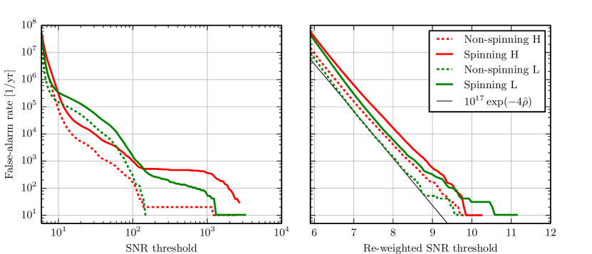
The spinning search clearly has a higher false-alarm rate for both detection statistics. As is well known from past CBC searches Blackburn et al. (2008), the SNR background exhibits a large tail associated with non-Gaussian transient glitches333Note that in our test we analyze all available science-mode data, including a few poor-quality data segments which a real search would exclude via data-quality flags Slutsky et al. (2010); Babak et al. (2013). Thus, the tail in our SNR background is likely exaggerated.. The spinning search seems to be affected more by glitches, as can be seen from the much larger tail at high SNR. Thanks to the effectiveness of the test, however, the re-weighted SNR is almost tail-free, although we find that strong glitches can still lead to false alarms noticeably stronger than what is typical in stationary Gaussian noise. The increase of false-alarm rate associated with the re-weighted SNR is proportional to the increase in number of templates () for almost all values of the threshold. Applying a fixed threshold in false-alarm rate implies an increase in single-detector re-weighted SNR of 0.5 or less when going from the non-spinning to the spinning search. The background distribution of re-weighted SNR falls approximately like with , such that if the total rate of triggers increases by a factor , the increase in statistic threshold required to compensate this increase (and thus preserve the same false-alarm rate) is only .
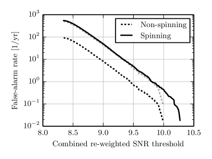
The coincident background distribution over the combined (quadrature sum) statistic is shown in Fig. 10. As for single-detector backgrounds, the larger false-alarm rate of the spinning search is consistent with the increase in template bank size except at very low rate, where our background sample is likely affected by a small number of loud glitches. Nevertheless, the increase in ranking statistic required to maintain a fixed false-alarm rate from non-spinning to spinning search is only about 0.3.
VI.2 Signal recovery and sensitivity
As a check of the correct behavior of the search, we first calculate the optimal SNR of each simulated source, i.e. the SNR obtained for a vanishing noise realization and a perfectly matched template. For each source producing a coincidence in both searches, we compare its combined optimal SNR with the combined SNR and re-weighted SNR actually recovered by the searches (the value for a zero noise realization and ideal template is also zero, thus the optimal re-weighted SNR is equal to the optimal SNR). We find that the non-spinning search fails to recover a noticeable fraction of both SNR and re-weighted SNR for , which is roughly consistent with the fitting factor calculations (Fig. 11, top and middle rows).
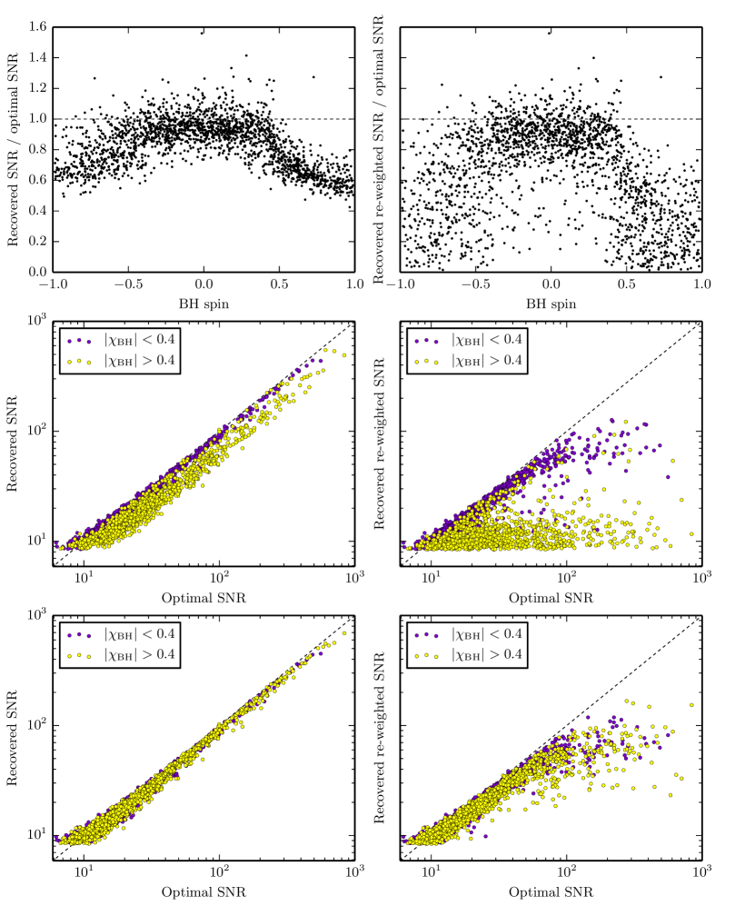
The impact of the test on spinning signals is particularly dramatic, as the loss in re-weighted SNR is much larger than the loss in SNR. The spinning search, instead, recovers the expected SNR almost completely, for all values of the BH spin (Fig. 11, bottom-left plot). Note however that sources with optimal SNR larger than have a significant loss in re-weighted SNR even in the spinning bank; in fact, the re-weighted SNR appears to asymptote to a finite value when the optimal SNR becomes very large (Fig. 11, bottom-right plot). This can be explained by the small but non-zero residual mismatch which is also present in the spinning bank. In fact, with any non-zero mismatch, at some (large) value of the statistic eventually starts growing like Allen et al. (2012). Combining this fact with the definition of re-weighted SNR (Eq. 8) results in a finite re-weighted SNR for arbitrarily large SNR.
Considering the relative sensitivity of the two searches at fixed false-alarm rate, we find that it depends strongly on the distribution of BH spins. Fig. 12 shows the receiver operating characteristic (ROC) curves for four populations of NS-BH binaries associated with different BH spin distributions. As done throughout this paper, all cases assume alignment between the BH spin and the orbital angular momentum.
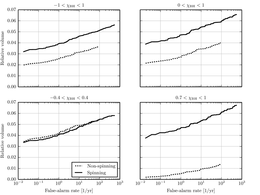
Assuming BHs can have any spin magnitude within the limits of the Kerr bound, we obtain an increase in sensitivity of the spinning search between 40% and 60% depending on the false-alarm rate. A slightly larger improvement is obtained if is restricted to be positive. If all BHs are highly spinning and positively aligned with the orbital angular momentum, however, the spinning search can be times more sensitive than the non-spinning one at interesting false-alarm rates. This large difference can be understood by considering the dramatic loss in re-weighted SNR of the non-spinning search, which is due in part to the large SNR loss and in part to the poor value of highly-spinning signals. If the search could be carried out using the standard SNR as the ranking statistic, or if we tuned the veto differently, the improvement could be significantly less dramatic, but likely still interesting; Fig. 8 (left plot) and Fig. 11 (top-left plot) both suggest a factor of when using the SNR as the ranking statistic. We also note that the improvement could be less dramatic if precession is included in the simulated binaries, but this will be studied in a forthcoming paper. For weakly spinning BHs (), the spinning search is a few percent less sensitive, as can be expected from the larger background, although the difference is comparable with the statistical fluctuations of our ROC curves.
Our signals provide insufficient statistics for studying the case of very small BH spins. Nevertheless, we can conclude with a back-of-the-envelope comparison of the searches assuming a worst-case population of exactly non-spinning BHs. Using the background curves from Fig. 10 and assuming a non-spinning search with detection threshold , the relative sensitive volume of the spinning search would be
| (16) |
In the worst case, therefore, the spinning search would lose 10% or less of the signals; the major burden would be the larger computational cost.
VII Conclusions
We show for the first time how an aligned-spin search for NS-BH binaries can be successfully implemented in the advanced detector era. We demonstrate a prototype search in the PyCBC framework which contains all the essential elements of a realistic CBC search: matched filtering with a template bank, signal-based vetoes, a suitable ranking statistic, coincidence, clustering, background estimates using time slides and sensitivity estimates via a simulated population of signals. The use of re-weighted SNR as event ranking statistic Abadie et al. (2012a) is sufficient to reduce the background to a level that makes the search more sensitive than traditional non-spinning searches over the full range of BH spins.
An important element in making this work is running the analysis on GPUs using PyCBC. The design of PyCBC and the available tools make it easy to put together such a pipeline, and the use of GPUs speeds up the analysis relative to using CPUs. Such an analysis would have been much harder with earlier technology.
Our spinning search has improved sensitivity relative to a traditional non-spinning search. The improvement in sensitivity depends strongly on the exact distribution of BH spins. If the magnitude of the dimensionless BH spins (taken to be parallel to the orbital angular momentum) is mostly below , the spinning and non-spinning searches have approximately the same sensitivity, despite the fact that the spinning template bank contains many more templates. If the BH spin is distributed uniformly in the range , then the spinning search has approximately greater astrophysical reach as measured by sensitive volume. The increase is one order of magnitude if the spin is uniformly distributed in the interval . We stress that these results assume that i) all systems are non-precessing, and ii) the BH and NS mass distributions are Gaussians with means and and standard deviations and respectively, with the additional constraints and . Although a careful study of the effect of different mass distributions is outside the scope of this paper, different distributions are unlikely to change the fact that a spinning search is more sensitive than a non-spinning search; this would require an unrealistic distribution restricted to the parameter-space region where the non-spinning bank performs well (see Fig. 8).
The available X-ray data and population synthesis studies suggest that the spin parameters of BHs may be reasonably large, greater than in the mass range we used. If this is the case, then for aligned systems an aligned spin search offers a significant improvement in sensitive volume and hence event rate, relative to traditional non-spinning searches. The improvement in search sensitivity could then mean the difference between detection and non-detection, depending on the astrophysical rate of NS-BH coalescence events.
We base our conclusions on an idealized noise PSD which could represent the early runs of advanced LIGO and we employ template banks fixed in time and identical between different detectors. We also show that the SNR loss of a non-spinning bank relative to a spinning one depends on the noise PSD. If advanced LIGO’s sensitivity has a significantly smaller bandwidth than our model, or if its noise PSD turns out to have a large variability over a time scale of a few months, the sensitivity of a search to spin effects could be smaller and thus our spinning search could be less beneficial. We argue however that these are unlikely scenarios, as the evolution of advanced LIGO will drive towards the large bandwidth of the final design sensitivity. In addition, if the bandwidth is so narrow that spin effects are less important than we find here, the spinning search would be at least as sensitive as the non-spinning one for a uniform distribution of BH spins and thus would only produce a larger computational cost.
The search methodology we present is straightforward and based on previous CBC analyses, but it has not been fully optimized. We expect that further improvements to the analysis will be possible. These include: i) constructing a better template bank using the full 3.5 pN phasing, a geometric placement algorithm and a mass- and spin-dependent upper frequency cutoff; ii) correcting the event ranking statistic to reflect the non-uniform distribution of templates over component masses and spins, as described in Dent and Veitch (2014); iii) improving the ranking statistic by accounting for event distributions over extrinsic parameters such as coalescence time and amplitude; and iv) tuning the coincidence and clustering steps. Including merger and ringdown effects should further improve the search sensitivity at the higher mass end of the parameter space. The impact of poor data quality on the computing time of inspiral jobs deserves further research. Improved data conditioning techniques such as gating, i.e. appropriately windowing out the data segment in the vicinity of high-amplitude glitches, are under investigation. In developing and testing such improvements to the search, PyCBC will be an essential tool. Finally, investigating the effects of precession will be important as well. This search should be seen as an intermediate step towards a full precessing search; a study is underway to quantify how well the current pipeline performs in detecting precessing signals.
Our conclusions remain robust towards further tuning: when using a template bank that includes the effect of spin, with a signal-based veto such as and the infrastructure required to run a search to completion, the gain in signal sensitivity easily outweighs the increase in background. Thus we advise an aligned-spin search rather than a non-spinning search for NS-BH binaries, even for the early advanced detectors.
Acknowledgements.
We thank Gergely Debreczeni, Mate Ferenc Nagy, Frank Ohme, Gianluca Guidi and Richard O’Shaughnessy for useful discussions and comments, and Carsten Aulbert and Oliver Bock for valuable support in using the Atlas cluster and MongoDB at the Albert Einstein Institute. We also thank the LIGO collaboration for providing the recolored synthetic strain data we analyzed. TDC is supported by the International Max-Planck Research School on Gravitational-Wave Astronomy. AJM and JLW are supported in part by the Pursuit program and Office of Undergraduate Research of ACU. This work is supported by National Science Foundation awards PHY-0847611, PHY-0854812, and a Cottrell Scholar award from the Research Corporation for Science Advancement. Part of the computations used in this work were performed on the Syracuse University Gravitation and Relativity cluster, which is supported by NSF awards PHY-1040231 and PHY-1104371. This paper has LIGO document number LIGO-P1400053.References
- Harry (2010) G. M. Harry (LIGO Scientific Collaboration), Class.Quant.Grav. 27, 084006 (2010).
- Accadia et al. (2012) T. Accadia et al. (VIRGO Collaboration), JINST 7, P03012 (2012).
- Somiya (2012) K. Somiya (KAGRA Collaboration), Class.Quant.Grav. 29, 124007 (2012), arXiv:1111.7185 [gr-qc] .
- Iyer et al. (2011) B. Iyer, T. Souradeep, C. Unnikrishnan, S. Dhurandhar, S. Raja, and A. Sengupta, “Ligo-india, proposal of the consortium for indian initiative in gravitational-wave observations (indigo),” https://dcc.ligo.org/cgi-bin/DocDB/ShowDocument?docid=75988 (2011).
- Abadie et al. (2010a) J. Abadie et al. (LIGO Scientific Collaboration, Virgo Collaboration), Class.Quant.Grav. 27, 173001 (2010a), arXiv:1003.2480 [astro-ph.HE] .
- Abbott et al. (2008) B. Abbott et al. (LIGO Scientific Collaboration), Phys. Rev. D78, 042002 (2008), arXiv:0712.2050 [gr-qc] .
- Aasi et al. (2013a) J. Aasi et al. (LIGO Scientific Collaboration, Virgo Collaboration), Phys. Rev. D87, 022002 (2013a), arXiv:1209.6533 [gr-qc] .
- Van Den Broeck et al. (2009) C. Van Den Broeck, D. A. Brown, T. Cokelaer, I. Harry, G. Jones, et al., Phys. Rev. D80, 024009 (2009), arXiv:0904.1715 [gr-qc] .
- Privitera et al. (2014) S. Privitera, S. R. P. Mohapatra, P. Ajith, K. Cannon, N. Fotopoulos, et al., Phys. Rev. D89, 024003 (2014), arXiv:1310.5633 [gr-qc] .
- Brown et al. (2012) D. A. Brown, I. Harry, A. Lundgren, and A. H. Nitz, Phys. Rev. D86, 084017 (2012), arXiv:1207.6406 [gr-qc] .
- Harry et al. (2013) I. Harry, A. Nitz, D. A. Brown, A. Lundgren, E. Ochsner, et al., (2013), arXiv:1307.3562 [gr-qc] .
- Mandel and O’Shaughnessy (2010) I. Mandel and R. O’Shaughnessy, Class.Quant.Grav. 27, 114007 (2010), arXiv:0912.1074 [astro-ph.HE] .
- O’Shaughnessy et al. (2005) R. W. O’Shaughnessy, J. Kaplan, V. Kalogera, and K. Belczynski, Astrophys.J. 632, 1035 (2005), arXiv:astro-ph/0503219 [astro-ph] .
- Eichler et al. (1989) D. Eichler, M. Livio, T. Piran, and D. N. Schramm, Nature (London) 340, 126 (1989).
- Narayan et al. (1992) R. Narayan, B. Paczynski, and T. Piran, Astrophys. J. 395, L83 (1992), astro-ph/9204001 .
- Ferrari et al. (2010) V. Ferrari, L. Gualtieri, and F. Pannarale, Phys. Rev. D 81, 064026 (2010).
- Pannarale et al. (2011) F. Pannarale, L. Rezzolla, F. Ohme, and J. S. Read, Phys. Rev. D84, 104017 (2011), arXiv:1103.3526 [astro-ph.HE] .
- Etienne et al. (2008) Z. B. Etienne, J. A. Faber, Y. T. Liu, S. L. Shapiro, K. Taniguchi, and T. W. Baumgarte, Phys. Rev. D 77, 084002 (2008).
- Etienne et al. (2009) Z. B. Etienne, Y. T. Liu, S. L. Shapiro, and T. W. Baumgarte, Phys. Rev. D 79, 044024 (2009).
- Duez et al. (2008) M. D. Duez, F. Foucart, L. E. Kidder, H. P. Pfeiffer, M. A. Scheel, and S. A. Teukolsky, Phys. Rev. D 78, 104015 (2008).
- Shibata and Uryū (2006) M. Shibata and K. Uryū, Phys. Rev. D 74, 121503 (2006).
- Löffler et al. (2006) F. Löffler, L. Rezzolla, and M. Ansorg, Phys. Rev. D 74, 104018 (2006).
- Apostolatos et al. (1994) T. A. Apostolatos, C. Cutler, G. J. Sussman, and K. S. Thorne, Phys. Rev. D49, 6274 (1994).
- Apostolatos (1995) T. Apostolatos, Phys. Rev. D52, 605 (1995).
- Apostolatos (1996) T. A. Apostolatos, Phys. Rev. D54, 2421 (1996).
- Buonanno et al. (2003) A. Buonanno, Y.-b. Chen, and M. Vallisneri, Phys. Rev. D67, 104025 (2003), arXiv:gr-qc/0211087 [gr-qc] .
- Grandclement et al. (2003) P. Grandclement, V. Kalogera, and A. Vecchio, Phys. Rev. D67, 042003 (2003), arXiv:gr-qc/0207062 [gr-qc] .
- Allen (2005) B. Allen, Phys. Rev. D71, 062001 (2005), arXiv:gr-qc/0405045 [gr-qc] .
- Babak et al. (2013) S. Babak, R. Biswas, P. Brady, D. Brown, K. Cannon, et al., Phys. Rev. D87, 024033 (2013), arXiv:1208.3491 [gr-qc] .
- Abbott et al. (2009a) B. Abbott et al. (LIGO Scientific Collaboration), Phys. Rev. D79, 122001 (2009a), arXiv:0901.0302 [gr-qc] .
- Abadie et al. (2012a) J. Abadie et al. (LIGO Collaboration, Virgo Collaboration), Phys. Rev. D85, 082002 (2012a), arXiv:1111.7314 [gr-qc] .
- Abadie et al. (2011) J. Abadie et al. (LIGO Scientific Collaboration, Virgo Collaboration), Phys. Rev. D83, 122005 (2011), arXiv:1102.3781 [gr-qc] .
- Abadie et al. (2010b) J. Abadie et al. (LIGO Scientific Collaboration, Virgo Collaboration), Phys. Rev. D82, 102001 (2010b), arXiv:1005.4655 [gr-qc] .
- Abbott et al. (2009b) B. Abbott et al. (LIGO Scientific Collaboration), Phys. Rev. D80, 047101 (2009b), arXiv:0905.3710 [gr-qc] .
- Abbott et al. (2006) B. Abbott et al. (LIGO Scientific Collaboration, http://www.ligo.org and TAMA Collaboration), Phys. Rev. D 73, 102002 (2006).
- Abbott et al. (2004) B. Abbott et al. ((LIGO Scientific Collaboration)), Phys. Rev. D 69, 122001 (2004).
- Abbott et al. (2005a) B. Abbott et al. (LIGO Scientific Collaboration), Phys. Rev. D 72, 082001 (2005a).
- Abbott et al. (2005b) B. Abbott et al. (LIGO Scientific Collaboration), Phys. Rev. D 72, 082002 (2005b).
- Abadie et al. (2010c) J. Abadie et al. (LIGO Scientific Collaboration, Virgo Collaboration), The Astrophysical Journal 715, 1453 (2010c).
- Aasi et al. (2013b) J. Aasi et al. (LIGO Scientific Collaboration, Virgo Collaboration), (2013b), arXiv:1304.0670 [gr-qc] .
- Thorne (1974) K. S. Thorne, Astrophys.J. 191, 507 (1974).
- McClintock et al. (2013) J. E. McClintock, R. Narayan, and J. F. Steiner, (2013), arXiv:1303.1583 [astro-ph.HE] .
- Dominik et al. (2012) M. Dominik, K. Belczynski, C. Fryer, D. Holz, E. Berti, et al., Astrophys.J. 759, 52 (2012), arXiv:1202.4901 [astro-ph.HE] .
- Lo and Lin (2011) K.-W. Lo and L.-M. Lin, Astrophys.J. 728, 12 (2011), arXiv:1011.3563 [astro-ph.HE] .
- Wagoner (1984) R. Wagoner, Astrophys.J. 278, 345 (1984).
- Bildsten (1998) L. Bildsten, Astrophys.J. 501, L89 (1998), arXiv:astro-ph/9804325 [astro-ph] .
- Chakrabarty et al. (2003) D. Chakrabarty, E. H. Morgan, M. P. Muno, D. K. Galloway, R. Wijnands, et al., Nature 424, 42 (2003), arXiv:astro-ph/0307029 [astro-ph] .
- Damour et al. (2012) T. Damour, A. Nagar, and L. Villain, Phys. Rev. D85, 123007 (2012), arXiv:1203.4352 [gr-qc] .
- Belczynski et al. (2007) K. Belczynski, R. E. Taam, E. Rantsiou, and M. van der Sluys, Astrophys.J. (2007), arXiv:astro-ph/0703131 [ASTRO-PH] .
- Kalogera (2000) V. Kalogera, Astrophys.J. 541, 319 (2000), arXiv:astro-ph/9911417 [astro-ph] .
- Lundgren and O’Shaughnessy (2013) A. Lundgren and R. O’Shaughnessy, (2013), arXiv:1304.3332 [gr-qc] .
- Foucart et al. (2013) F. Foucart, M. B. Deaton, M. D. Duez, L. E. Kidder, I. MacDonald, et al., Phys. Rev. D87, 084006 (2013), arXiv:1212.4810 [gr-qc] .
- Pan et al. (2011) Y. Pan, A. Buonanno, M. Boyle, L. T. Buchman, L. E. Kidder, et al., Phys. Rev. D84, 124052 (2011), arXiv:1106.1021 [gr-qc] .
- Brown et al. (2013) D. A. Brown, P. Kumar, and A. H. Nitz, Phys. Rev. D87, 082004 (2013), arXiv:1211.6184 [gr-qc] .
- pyc (a) “PyCBC,” https://www.lsc-group.phys.uwm.edu/daswg/projects/pycbc.html (a).
- (56) “The LIGO Algorithms Library,” https://www.lsc-group.phys.uwm.edu/daswg/projects/lalsuite.html.
- Aasi et al. (2014) J. Aasi et al. (The LIGO Scientific Collaboration, the Virgo Collaboration, the NINJA-2 Collaboration), (2014), arXiv:1401.0939 [gr-qc] .
- Allen et al. (2012) B. Allen, W. G. Anderson, P. R. Brady, D. A. Brown, and J. D. Creighton, Phys. Rev. D85, 122006 (2012), arXiv:gr-qc/0509116 [gr-qc] .
- Percival and Walden (1993) D. Percival and A. Walden, Spectral Analysis for Physical Applications: Multitaper and Conventional Univariate Techniques (Cambridge University Press, Cambridge, UK, 1993).
- Abadie et al. (2012b) J. Abadie et al. (Virgo Collaboration, LIGO Scientific Collaboration), (2012b), arXiv:1203.2674 [gr-qc] .
- Cutler and Flanagan (1994) C. Cutler and E. E. Flanagan, Phys. Rev. D 49, 2658 (1994).
- (62) “The Python Programming Language,” http://www.python.org.
- (63) “SWIG,” http://www.swig.org.
- (64) “CUDA,” http://www.nvidia.com/object/cuda_home_new.html.
- (65) “OpenCL,” https://www.khronos.org/opencl.
- pyc (b) “PyCUDA,” http://mathema.tician.de/software/pycuda (b).
- (67) “PyOpenCL,” http://mathema.tician.de/software/pyopencl.
- (68) “cuFFT,” https://developer.nvidia.com/cuFFT.
- Frigo and Johnson (2005) M. Frigo and S. G. Johnson, Proceedings of the IEEE 93, 216 (2005), special issue on “Program Generation, Optimization, and Platform Adaptation”.
- (70) “MKL,” http://software.intel.com/en-us/intel-mkl.
- (71) “The Atlas Computational Cluster,” https://wiki.atlas.aei.uni-hannover.de/foswiki/bin/view/ATLAS/WebHome.
- (72) “NVIDIA System Management Interface,” https://developer.nvidia.com/nvidia-system-management-interface.
- Harry et al. (2009) I. W. Harry, B. Allen, and B. Sathyaprakash, Phys. Rev. D80, 104014 (2009), arXiv:0908.2090 [gr-qc] .
- Babak (2008) S. Babak, Class.Quant.Grav. 25, 195011 (2008), arXiv:0801.4070 [gr-qc] .
- Blanchet et al. (1995) L. Blanchet, T. Damour, B. R. Iyer, C. M. Will, and A. G. Wiseman, Phys. Rev. Lett. 74, 3515 (1995).
- Blanchet et al. (2004) L. Blanchet, T. Damour, G. Esposito-Farèse, and B. R. Iyer, Phys. Rev. Lett. 93, 091101 (2004).
- Arun et al. (2009) K. Arun, A. Buonanno, G. Faye, and E. Ochsner, Phys. Rev. D79, 104023 (2009), arXiv:0810.5336 [gr-qc] .
- Kidder (1995) L. E. Kidder, Phys. Rev. D 52, 821 (1995).
- Blanchet et al. (2006) L. Blanchet, A. Buonanno, and G. Faye, Phys. Rev. D 74, 104034 (2006).
- Baird et al. (2013) E. Baird, S. Fairhurst, M. Hannam, and P. Murphy, Phys. Rev. D 87, 024035 (2013).
- Sengupta et al. (2003) A. S. Sengupta, S. Dhurandhar, and A. Lazzarini, Phys. Rev. D67, 082004 (2003), arXiv:gr-qc/0301025 [gr-qc] .
- Ohme et al. (2013) F. Ohme, A. B. Nielsen, D. Keppel, and A. Lundgren, Phys. Rev. D88, 042002 (2013), arXiv:1304.7017 [gr-qc] .
- Pan et al. (2004) Y. Pan, A. Buonanno, Y.-b. Chen, and M. Vallisneri, Phys. Rev. D69, 104017 (2004), arXiv:gr-qc/0310034 [gr-qc] .
- Marsat et al. (2013) S. Marsat, A. Bohe, G. Faye, and L. Blanchet, Class. Quant. Grav. 30, 055007 (2013), arXiv:1210.4143 [gr-qc] .
- Wade et al. (2013) M. Wade, J. D. E. Creighton, E. Ochsner, and A. B. Nielsen, Phys. Rev. D 88, 083002 (2013).
- (86) “Mongo DB,” http://www.mongodb.org.
- Nielsen (2013) A. B. Nielsen, Class.Quant.Grav. 30, 075023 (2013), arXiv:1203.6603 [gr-qc] .
- Ozel et al. (2010) F. Ozel, D. Psaltis, R. Narayan, and J. E. McClintock, Astrophys.J. 725, 1918 (2010), arXiv:1006.2834 [astro-ph.GA] .
- Kiziltan et al. (2013) B. Kiziltan, A. Kottas, M. De Yoreo, and S. E. Thorsett, Astrophys.J. 778, 66 (2013), arXiv:1309.6635 [astro-ph.SR] .
- Finn and Chernoff (1993) L. S. Finn and D. F. Chernoff, Phys. Rev. D47, 2198 (1993), arXiv:gr-qc/9301003 [gr-qc] .
- Blackburn et al. (2008) L. Blackburn, L. Cadonati, S. Caride, S. Caudill, S. Chatterji, et al., Class.Quant.Grav. 25, 184004 (2008), arXiv:0804.0800 [gr-qc] .
- Slutsky et al. (2010) J. Slutsky, L. Blackburn, D. Brown, L. Cadonati, J. Cain, et al., Class.Quant.Grav. 27, 165023 (2010), arXiv:1004.0998 [gr-qc] .
- Dent and Veitch (2014) T. Dent and J. Veitch, Phys. Rev. D 89, 062002 (2014).