Efficient DMFT impurity solver using real-time dynamics with Matrix Product States
Abstract
We propose to calculate spectral functions of quantum impurity models using the Time Evolving Block Decimation (TEBD) for Matrix Product States. The resolution of the spectral function is improved by a so-called linear prediction approach. We apply the method as an impurity solver within the Dynamical Mean Field Theory (DMFT) for the single- and two-band Hubbard model on the Bethe lattice. For the single-band model we observe sharp features at the inner edges of the Hubbard bands. A finite size scaling shows that they remain present in the thermodynamic limit. We analyze the real time-dependence of the double occupation after adding a single electron and observe oscillations at the same energy as the sharp feature in the Hubbard band, indicating a long-lived coherent superposition of states that correspond to the Kondo peak and the side peaks. For a two-band Hubbard model we observe an even richer structure in the Hubbard bands, which cannot be related to a multiplet structure of the impurity, in addition to sharp excitations at the band edges of a type similar to the single-band case.
I introduction
The field of strongly correlated materials has experienced vast growth during the last three decades. Electronic correlations pose a particular challenge for theory, and many phenomena such as high-temperature superconductivity have eluded a proper understanding to this day. A correlation phenomenon that is non trivial but nonetheless fully understood is the Kondo effect Kondo (1964); Wilson (1975). The Kondo model and its cousin, the Anderson impurity model, are not only relevant for its original purpose, i.e., for magnetic impurities in solids, but also for quantum dots Kouwenhoven and Glazman (2001) and even for bulk materials. For the latter, dynamical mean-field theory (DMFT) Metzner and Vollhardt (1989); Georges et al. (1996); Georges (2004) maps a bulk lattice model onto the self-consistent solution of an Anderson impurity model and includes in this way a major part of electronic correlations, namely the local ones.
Strong electronic correlations make the computational cost of directly solving the Schrödinger equation prohibitively large, and advanced numerical methods, often approximate ones, are in many cases the only viable option. At the forefront of these methods lie the Quantum Monte-Carlo (QMC) technique Assaad and Evertz (2008); Gull et al. (2011), the Numerical Renormalization Group Bulla et al. (2008); Wilson (1975), the Density Matrix Renormalization Group (DMRG) White (1992, 1993); Schollwöck (2011), cluster approaches like Cluster Perturbation Theory Sénéchal et al. (2000) and the Variational Cluster Approach Potthoff et al. (2003) and DMFT Metzner and Vollhardt (1989); Georges et al. (1996); Georges (2004). All these methods have their strengths and weaknesses. QMC gives formally the exact solution, but is in practice plagued by statistical errors and the sign-problem. The NRG excels at capturing the low-energy physics, but has a hard time to resolve high-energy features in the spectrum and is restricted to impurity problems. The DMRG can treat both the low- and high-energy scale on equal footing, but is best suited for 1-dimensional (1d) models. Methods for higher dimensional (d1) problems are scarce. One of the most promising among these is the DMFT Georges et al. (1996) which becomes exact in the limit d Metzner and Vollhardt (1989) and which yields an approximation for the finite dimensional lattice. The key quantity of DMFT is the local lattice spectral function which is calculated self-consistently. The framework of DMFT is readily established Georges et al. (1996), but the actual solution of the DMFT equations is complicated: it involves the calculation of the spectral function of an interacting impurity system which even for single-band models is highly non-trivial, and the complexity grows quickly with the number of considered bands (i.e. impurity orbitals). Many different approaches have been proposed to tackle the problem. The most common ones are QMC Jarrell (1992); Rozenberg et al. (1992); Gull et al. (2011); Parcollet et al. (2015); Boehnke et al. (2011); Parragh et al. (2012), exact diagonalization (ED) Caffarel and Krauth (1994); Sangiovanni et al. (2006); Granath and Strand (2012); Lu et al. (2014), and NRG Žitko and Pruschke (2009); Pruschke and Bulla (2005); Bulla (1999). QMC can efficiently handle multiple bands, but when formulated in imaginary time, it lacks high resolution of the spectral function. This is mainly attributable to the ill-conditioned analytic continuation from imaginary to real frequencies. Based on the work in Refs. Mühlbacher and Rabani (2008); Werner et al. (2009), the QMC method has recently been extended to the calculation of real-frequency spectra using bold line methods Prokof’ev and Svistunov (2007); Gull et al. (2010) (see Refs. Cohen et al. (2014a, b) and references therein). The analytic continuation is then traded for the introduction of a sign-problem. ED naturally works with real energies, but it is severely limited by the number of possible sites. This again reduces the spectral resolution considerably. Recently, two extensions to the ED method have been put forward Granath and Strand (2012); Lu et al. (2014) which increase the possible resolution of the spectral function Granath and Schött (2014). The NRG on the other hand, being designed for impurity problems, achieves very good spectral resolution at small energies. But due to a necessarily logarithmic discretization Bulla et al. (2008) of the bath density of states (DOS), high energy features of the bath are increasingly hard to resolve, which is also likely to affect the fixed point of the DMFT-iteration. In addition, NRG has an intrinsic exponential growth of complexity with the number of bands of the underlying lattice model. More than two bands Greger et al. (2013); Pruschke and Bulla (2005) have so far been unfeasible. The DMRG on the other hand offers several ways to be used as an impurity solver within the DMFT. One possible way is to employ the dynamical DMRG (DDMRG) Jeckelmann (2002); Kühner and White (1999) to obtain the DMFT-spectral function Peters (2011); Karski et al. (2008, 2005); Nishimoto et al. (2004), whereas other approaches use a continued fraction expansion of the Greens function García et al. (2004); Hallberg (1995). The broad application of DDMRG as an impurity solver is though hindered by the fact that one has to perform a separate DMRG run for each frequency and to perform the inversion of an ill-conditioned system of linear equations, which can become very time consuming. Recently, the Chebyshev expansion technique Holzner et al. (2011); Weiße et al. (2006) has been proposed by some of us Ganahl et al. (2014) as an impurity solver for DMFT. Advantages are that it works at zero temperature, that no inversion problem has to be solved, and that the spectral function can be calculated with uniform resolution and high precision for all in a single run. This reduces computational costs considerably, but on the other hand it is not straightforward to parallelize the method. In the present work we propose to employ the Time Evolving Block Decimation (TEBD) Vidal (2004, 2003) for Matrix Product States (MPS) Schollwöck (2011); Verstraete et al. (2008) to compute the spectral function. We combine it with a so called linear prediction technique White and Affleck (2008); Barthel et al. (2009); Ganahl et al. (2014) to improve on the spectral resolution. Our method shares the advantages of the Chebyshev approach, but it can be carried out without the need of explicitly adding states. By employing a Suzuki-Trotter decomposition it can easily be parallelized and is therefore both a very precise and very efficient method. We note that the numerical costs of the Chebyshev technique and time evolution both scale as , where is the local Hilbert space dimension and is the matrix dimension employed. The prefactor however depends strongly on the parameters used in the two approaches. For a recent improvement of the Chebyshev technique see Wolf et al. (2015). For the case of the single-band Hubbard model, the run time of the time evolution method in our implementation was smaller by roughly an order of magnitude.
We apply it as a DMFT impurity solver for the single and the two-band Hubbard model on the Bethe lattice.
II Models
II.1 One-band Hubbard Model
In this work we adress the computation of the local Greens function of the Hubbard model on the Bethe lattice using DMFT. In the limit of no interaction the model has a semi circular density of states (DOS) with a bandwidth of . The central ingredient in DMFT is the iterative calculation of the spectral function of an impurity model. We consider the Single Impurity Anderson Model (SIAM)
| (1) |
where are fermionic annihilation and creation operators of spin at the impurity site, and are the interaction and the local potential of the underlying lattice model, i.e. the single-band Hubbard model, and and are variational parameters which are optimized during the DMFT cycles (see below). We assume a spin-symmetric coupling and bath-dispersion , and work at particle-hole symmetry , in which case is independent of spin. We thus omit the spin variable henceforth and simply write .
Greens and spectral functions can be calculated from the real time evolution and subsequent Fourier transformation of
| (2) |
to
| (3) |
Here is given in the Heisenberg picture, and is a non-degenerate ground state at zero energy. Due to the hermiticity of , the function is real and normalized to unity. One way to obtain is to calculate the two quantities
| (4) |
for and Fourier-transform them. Using
| (5) |
where the second line is valid only at particle hole symmetry, the spectral function can be expressed as
| (6) |
To obtain the spectral function at particle-hole symmetry, we thus only need to calculate for , as the real part of is even in .
II.2 Two-band Hubbard Model
The most promising feature of the method is its applicability to multi-band systems. We will demonstrate this by applying it as an impurity solver for the symmetric two-band Hubbard model Pruschke and Bulla (2005); Koga et al. (2002); Han et al. (1998); Held and Vollhardt (1998) on the Bethe lattice. Under the assumption that the bath is spin symmetric the resulting effective impurity model assumes the form with
| (7a) | ||||
| (7b) | ||||
with , and we choose throughout. Here, is a fermionic annihilation operator of the correlated orbital at the impurity site, are the corresponding particle number operators, and and are the bath-electron annihilation and particle number operators for , respectively. Symbols and denote complementary variables, e.g. if , then , and similar for . Note that we use a fully rotational invariant interaction with all spin-flip and pair-hopping terms included.
III Methods
III.1 Dynamical mean field theory
In this paper we address the single- and two-band Hubbard model on the Bethe lattice. This is convenient for two reasons: (i) the DMFT yields exact results in this case, and (ii) the DMFT self-consistency scheme is especially simple. The quantity of genuine interest in DMFT is the local lattice spectral function of an interacting, -dimensional lattice problem (e.g the Hubbard model on the Bethe lattice). At convergence it is identical to the impurity spectral function . The basic idea of DMFT is to mimic the effect of the interacting lattice surrounding a given site by a suitably chosen bath of free electrons. Interacting lattice site and surrounding bath yield an impurity problem described by Eq.(1) or Eq.(7). The bath can be represented by the hybridization function , with an imaginary part . The general outline of the DMFT cycle is as follows: For each correlated orbital on the impurity site we initially guess a , where is an iteration index. A set of SIAM parameters and is then obtained by discretizing as described in Ref.Bulla et al. (2008). We use a discretization scheme linear in energy in this work. The method can deal with any discretization. After the discretization the system has a linear chain geometry
| (8) |
with only nearest neighbor hopping and local potentials . The number of discretization parameters corresponds to the chain length . Using an impurity solver we calculate the impurity spectral function of Eq.(8), from which one obtains the new
| (9) |
with a mixing parameter (“underrelaxation”) that can be adjusted for faster convergence. Here, is the bandwidth of the non-interacting spectral function of the Bethe lattice. In the following, all results are given in units of . is then again discretized, and the loop is iterated upon convergence, i.e. until
| (10) |
For our calculations we enforce particle-hole and spin symmetry which results in in Eq.(8).
For the two-band Hubbard model we focus on the symmetric model in which at both bands have the same bandwidth . For the discretization we use a symmetric setup with two DMFT-baths of lengths . Each bath contains electrons of up and down spin character.
The two-band model has been frequently investigated in the past Greger et al. (2013); Pruschke and Bulla (2005); Held and Vollhardt (1998). Like the single-band model it exhibits a MI transition at a finite , for .Pruschke and Bulla (2005)
Using the NRG as an impurity solver Pruschke and Bulla (2005), it has been observed that a finite leads to a strong renormalization of the Kondo temperature and hence affects the MI transition. Obtaining accurate results, especially for the high energy features of the Hubbard bands remains a challenging problem.
III.2 Time Evolving Block Decimation
The essential task of the impurity solver in DMFT is to calculate the greater (or lesser) Greens function . We achieve this by calculating the ground state using the DMRG and subsequently employ the Time Evolving Block Decimation (TEBD) Vidal (2003, 2004) to evolve forward in time. We use a second order Trotter breakup with , and in the single-band case measure every 25 Trotter steps, thus , with . For the two-band model we split the calculation of the Greens function into two runs, one forward and one backward in time, which allows us to reach longer times and/or larger system sizes with a smaller computational effort Barthel (2013). From these runs we calculate the Greens function on a grid with grid-points , with . We then apply the linear prediction method (see below) to extrapolate 10000 further points. In the single-band case we also employ an unfolding procedure Saberi et al. (2008) to separate the spin degrees of freedom of the electrons into a left chain containing up spins and a right chain containing down spins which is computationally more efficient. In this case, the total length of the system is , that is each bath has a length of sites. A decoupling for two and more bands can be carried out in a similar spirit with multiple chains connected at the impurity site in a star-like geometry Holzner et al. (2010) where every chain carries a band and spin index. For the two-band case however, we only applied a decoupling of the orbital degrees of freedom. The impurity orbital is in this case located at the center of a chain, where the left sites contain the bath and impurity orbital, and the right sites the bath and impurity orbital. Each of the and bath orbitals contains electrons of up- and down-spin flavour.
In the TEBD, only a limited number of Schmidt-states and Schmidt-values can be kept at a certain bond connecting two sites, which is the major approximation of the method. The error of a single time step can be quantified by the truncated weight Vidal (2003); Schollwöck (2011)
| (11) |
obtained after truncating the state down to a matrix dimension , where is the local Hilbert space dimension. In our implementation of the TEBD, after every time step the matrix dimension is reduced just enough to obtain the prespecified . Additionally, we set a hard limit for the maximum matrix dimension of or in the single-band and or in two-band model.
III.3 Linear Prediction
The so called linear prediction technique Press et al. (2007); Ganahl et al. (2014); White and Affleck (2008); Barthel et al. (2009) is a very simple and powerful method for the extrapolation of time series. It amounts to describing the time series as a sum of many exponentials or, equivalently, the spectrum as a sum of many Lorentzians. On the basis of calculated data points , at equidistant times , one predicts data points for as a linear combination of the first data points:
| (12) |
One obtains the optimal by minimization of a cost function
| (13) |
which yields
| (14) | |||||
for . Eq. (14) is inverted using a pseudo-inverse with cutoff . Data points at () can then be predicted from
| (15) |
with
All spectral functions have been obtained by predicting 10000 further data points on top of computed data points. Due to the exponential dependence of in Eq.(15), any eigenvalue of that is larger than unity has to be either renormalized to unity or set to zero, in order to avoid divergence in the prediction Barthel et al. (2009); Ganahl et al. (2014). The interplay of and the eigenvalue rescaling is investigated in more detail in the appendix. There we show that zeroed eigenvalues yield better results.
The linear prediction algorithm has two parameters (“time window”) and (pseudo-inverse cutoff). From analysis of the dependence of the DMFT-fixed point on these parameters (see appendix), we found , and or smaller, in conjunction with setting large eigenvalues of the prediction matrix to 0, to yield good results. Unless stated otherwise, these parameter values were used to obtain the results in this paper.
IV Results
To verify our approach we benchmarked our results for the impurity spectral function of a SIAM with results of the dynamical DMRG Raas and Uhrig (2005), to our knowledge the most precise data available (see appendix), and found excellent agreement. In the following we present our results for the one and two-band Hubbard model.
IV.1 One-band Hubbard model
We start by applying our method to DMFT for the single-band Hubbard model on the Bethe lattice for interaction strengths and in the metallic region and and in the insulating region. We use . Fig. 1(a) and (b) show the results for and (red solid lines). At , distinct features at the inner edges of the Hubbard satellites start to emerge, as has been observed in previous DDMRG Karski et al. (2008, 2005) and NRG Žitko and Pruschke (2009) studies, in QMC calculations Gull et al. (2010) as well as in MPS calculations with Chebyshev moments Ganahl et al. (2014), and recently also in advanced ED calculations Granath and Schött (2014); Lu et al. (2014); Granath and Strand (2012). For comparison we show results obtained with the Chebyshev expansion technique Ganahl et al. (2014) (black dash-dotted lines). They are compatible with our present results. For values of and 3.6 we plot results in Fig. 1(c). In contrast to Fig. 1(a) and (b), we use a mixing parameter of in Fig. 1(c), which yields a smoother convergence to the insulating solution. If no mixing is applied, the spectra alternate between an insulating and a metallic solution with a tiny quasi-particle weight. This effect is particularly strong at close to the transition and is also enhanced when increasing or decreasing , which we attribute to Trotter and truncation effects in the time series. We note that in Fig. 1(c) there is some small residual spectral weight left in the gap region (of the order of ).

IV.2 Sharp peaks in the Hubbard bands
We proceed to study the metallic state in the coexistence region , where , and Karski et al. (2008). For such , the narrowing of the quasi-particle peak at and the appearance of sharp side peaks in the Hubbard band Ganahl et al. (2014); Lu et al. (2014); Granath and Strand (2012); Karski et al. (2005, 2008) make a high-resolution calculation of a challenging task.
In Fig. 2, we present for and a chain length of sites. We clearly observe a separation of energy-scales into a sharp resonance at and two broad Hubbard satellites at , decorated with two sharp features at the inner edges of the Hubbard peaks. The insets are closeups on the sharp side peak of the left Hubbard satellite (left) and the quasi-particle peak (right).

It can be shown analytically Hewson (1993) that the exact value of for all values of . This pinning of the height of the Kondo-resonance is fulfilled to good accuracy in our simulations. In Fig. 2 we analyze the convergence of the results with increasing precision of the MPS calculations. The latter is governed by the truncation error , related to the MPS matrix-dimension , which bounds the number of Schmidt states kept at each bi-partition during the simulation. Fig. 2 shows results for three different simulations. With increasing precision we initially observe a sharpening of the Hubbard side-peaks. From the plot we conclude that using already yields converged results. The magnetiztion of our DMRG ground state is zero to within accuracy, which rules out that these sharp excitations are artefacts from any spurious magnetic ordering due to the DMRG truncation. A slight decrease of the quality of the pinning criterion is most likely related to linear prediction inaccuracies.
A second important parameter is the chain length , which is directly related to the number of discretization points of the bath spectral function. In Fig. 3(a) we present DMFT-spectra for and different system sizes , with or and . With increasing system size , we observe a shift of the Hubbard side-peak position towards smaller (left inset Fig. 3), as well as a reduction of its height Karski et al. (2008, 2005). A similar reduction is observed in the height of the quasi-particle peak (right inset in Fig. 3), in violation of the pinning criterion. However, the DMFT self-consistency cycle is stable and still converges, and the violation does not increase during this cycle. We note that the spectral height at is the quantity which is most susceptible to small errors in the large time evolution in our method, more so than the spectrum at other frequencies.
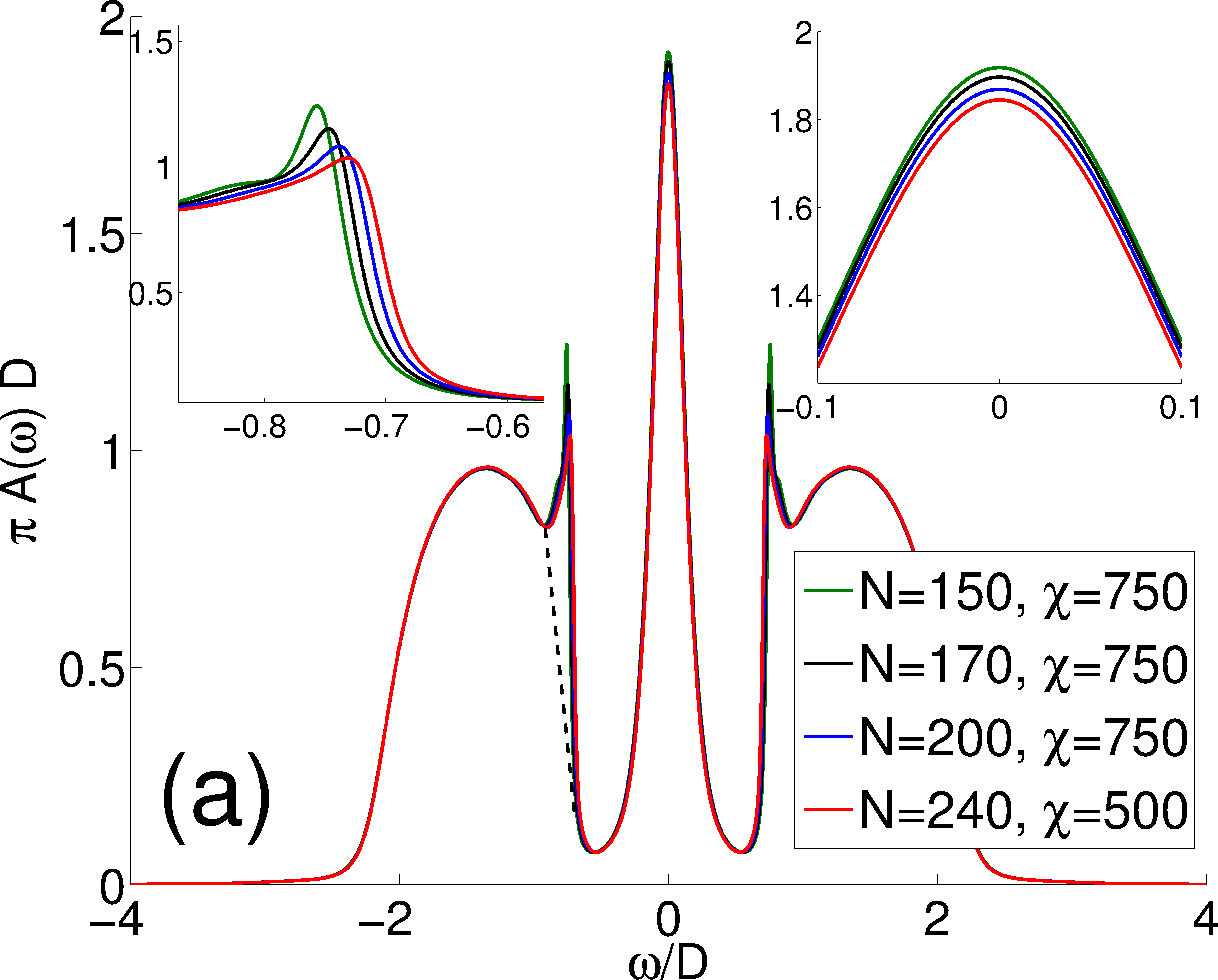
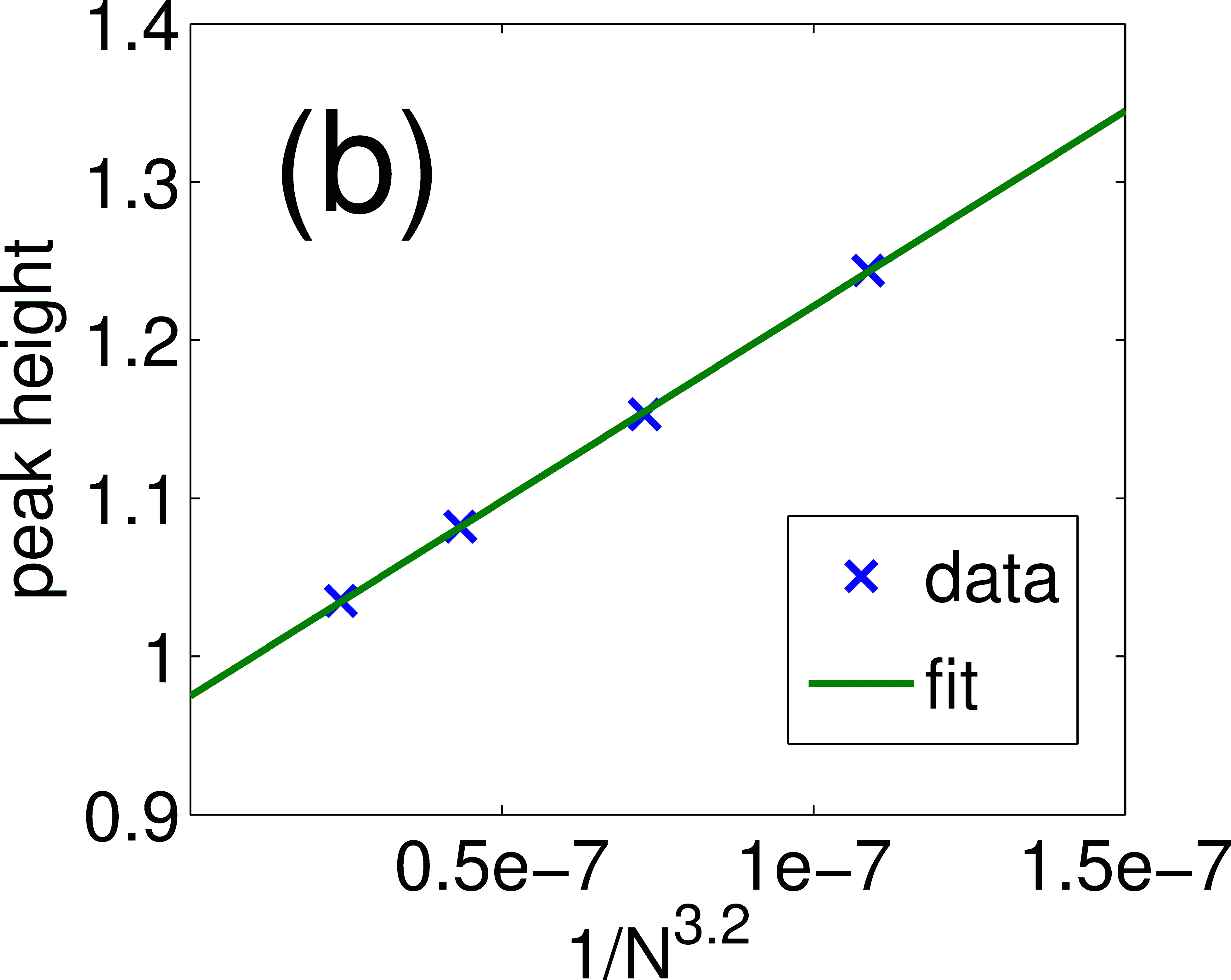
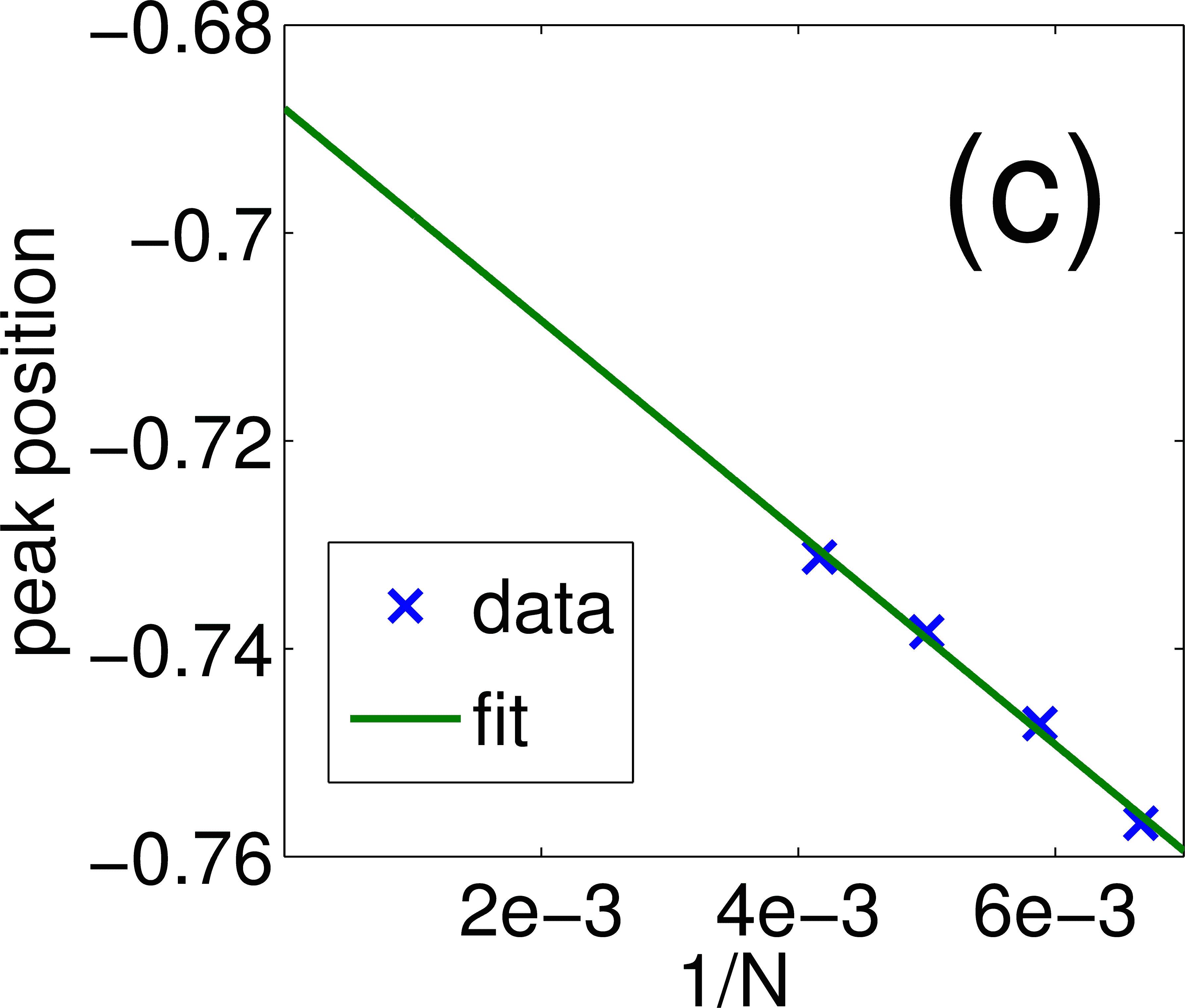
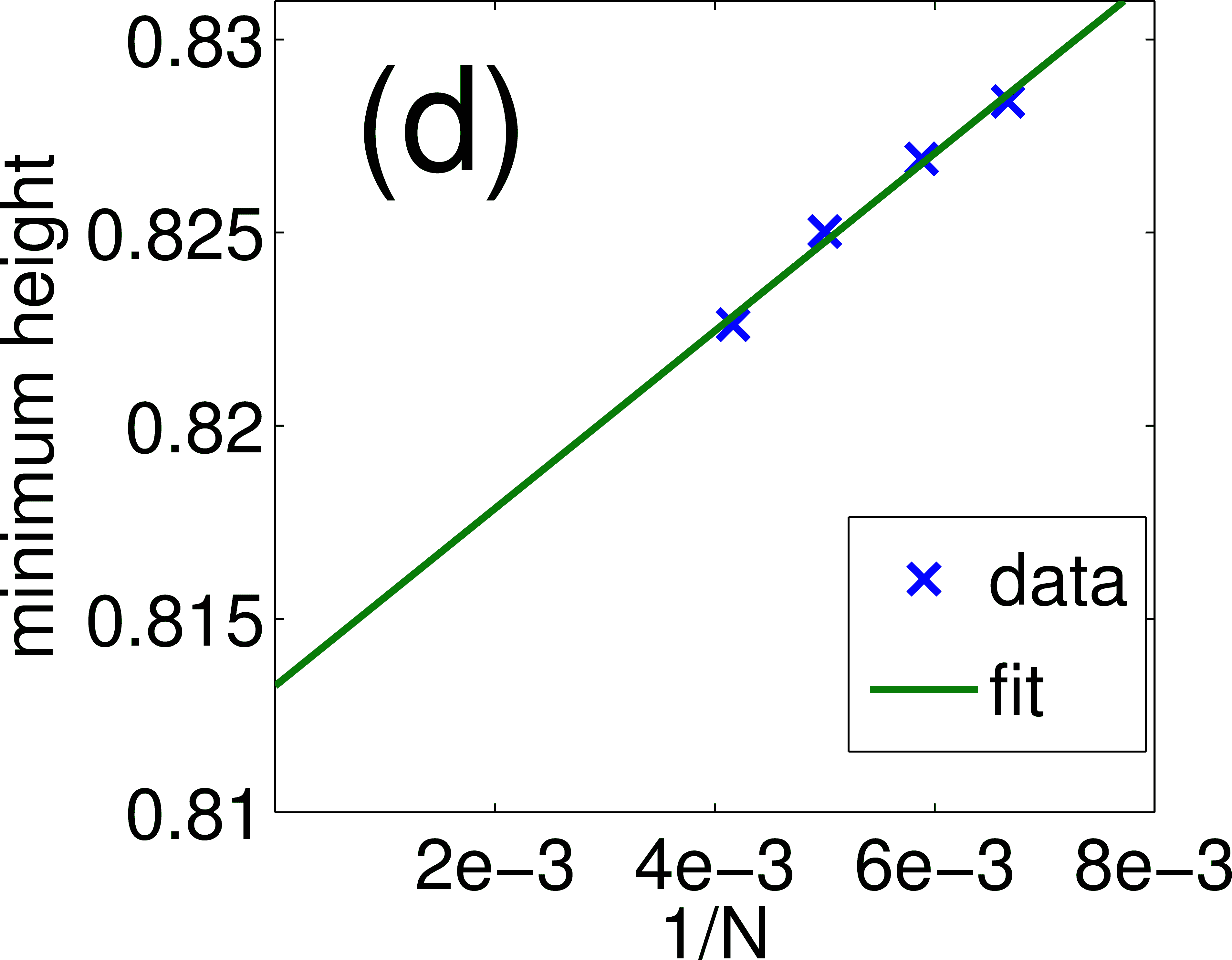
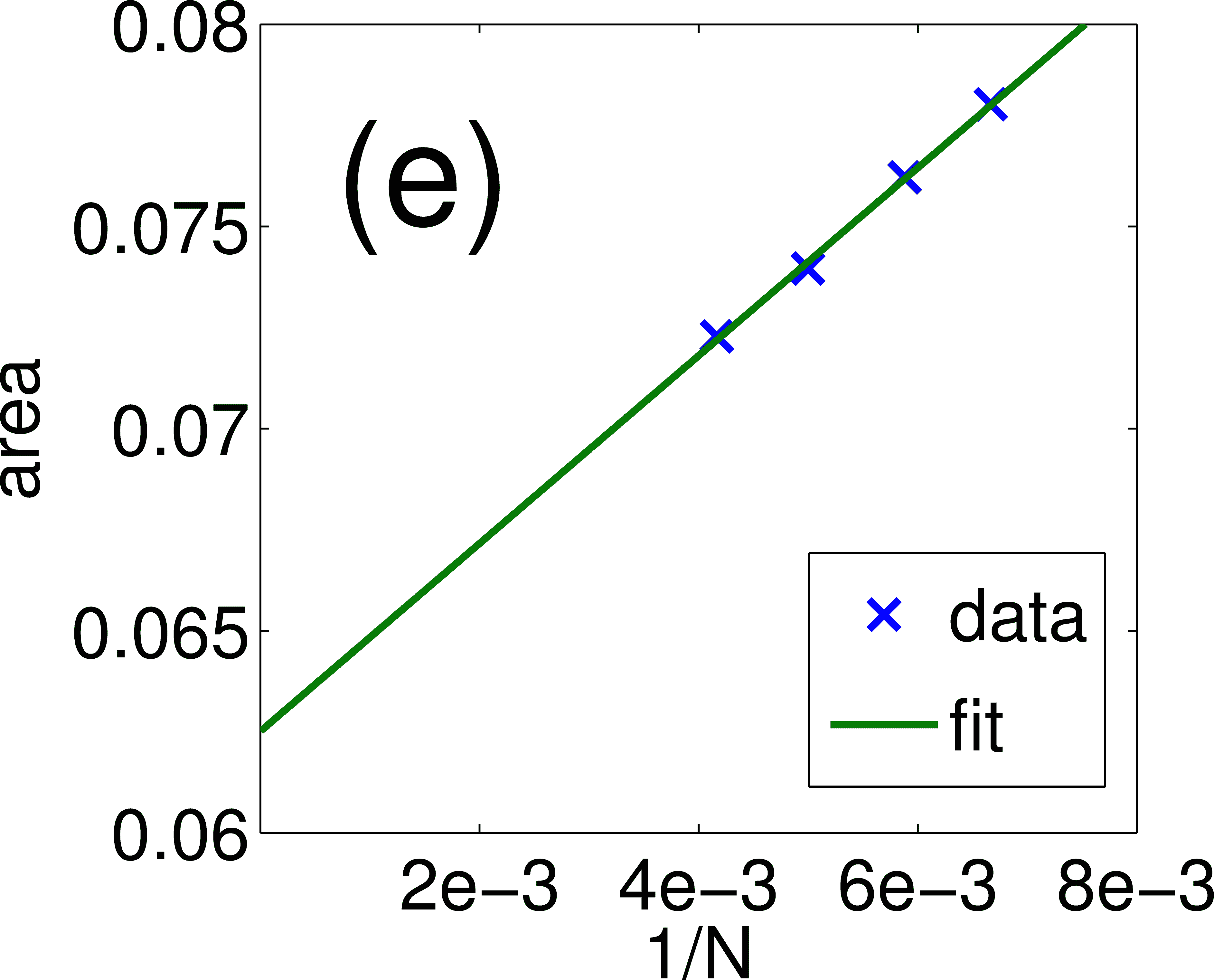
In Fig. 3(b) to (e) we display a finite size scaling of the side peaks, which demonstrates that they remain present in the infinite size limit. Fig. 3(b) shows a finite size scaling of the height of the side peak (the exponent was found to map the data to a straight line), and (c) a scaling of its position. In panel (d) we present a finite size scaling of the minimum to the left of the left side peak. Finally panel (e) shows a scaling of an approximate measure of the area of the side peak, namely the area between the left side peak and a straight line through the local minimum, tangent to spectrum at the global minimum (see dashed black line in the lower Hubbard band of the main panel in Fig. 3(a)). Since the height of the central peak is also size-dependent, the exact properties of the side peaks are likely to change with higher precision of the calculations. The important point (further strengthened by a slight curvature of the data) is that they converge to finite values, i.e. the side peaks remain present in the thermodynamic limit.
With increasing , the quasi particle peak is expected to narrow until it vanishes at Karski et al. (2005); Bulla (1999). In the main panel of Fig. 4 (a) we show results for . The right inset tracks the evolution of the quasi-particle peak for and 2.8. As expected, its weight is strongly reduced upon increasing . The Hubbard side-peak (left inset) is visibly shifted towards smaller , and it becomes sharper. in agreement with the DDMRG data of Refs. Karski et al. (2008, 2005); Ganahl et al. (2014), In the NRG study in Ref. Žitko and Pruschke, 2009 the side peak shows narrowing but shrinks quickly when approaching the transition, while in the ED study in Ref. Lu et al., 2014, data for is not available, and does not allow a conclusive study of the side peak weight and height. In the region between the quasi particle peak and the side-peak we observe a reduction of the spectral weight with increasing . We note that we also observe the appearance of a second, smaller side peak close to the first one for . The height of this peak is however much larger for smaller chains (not shown), so that it may be a finite size artifact.

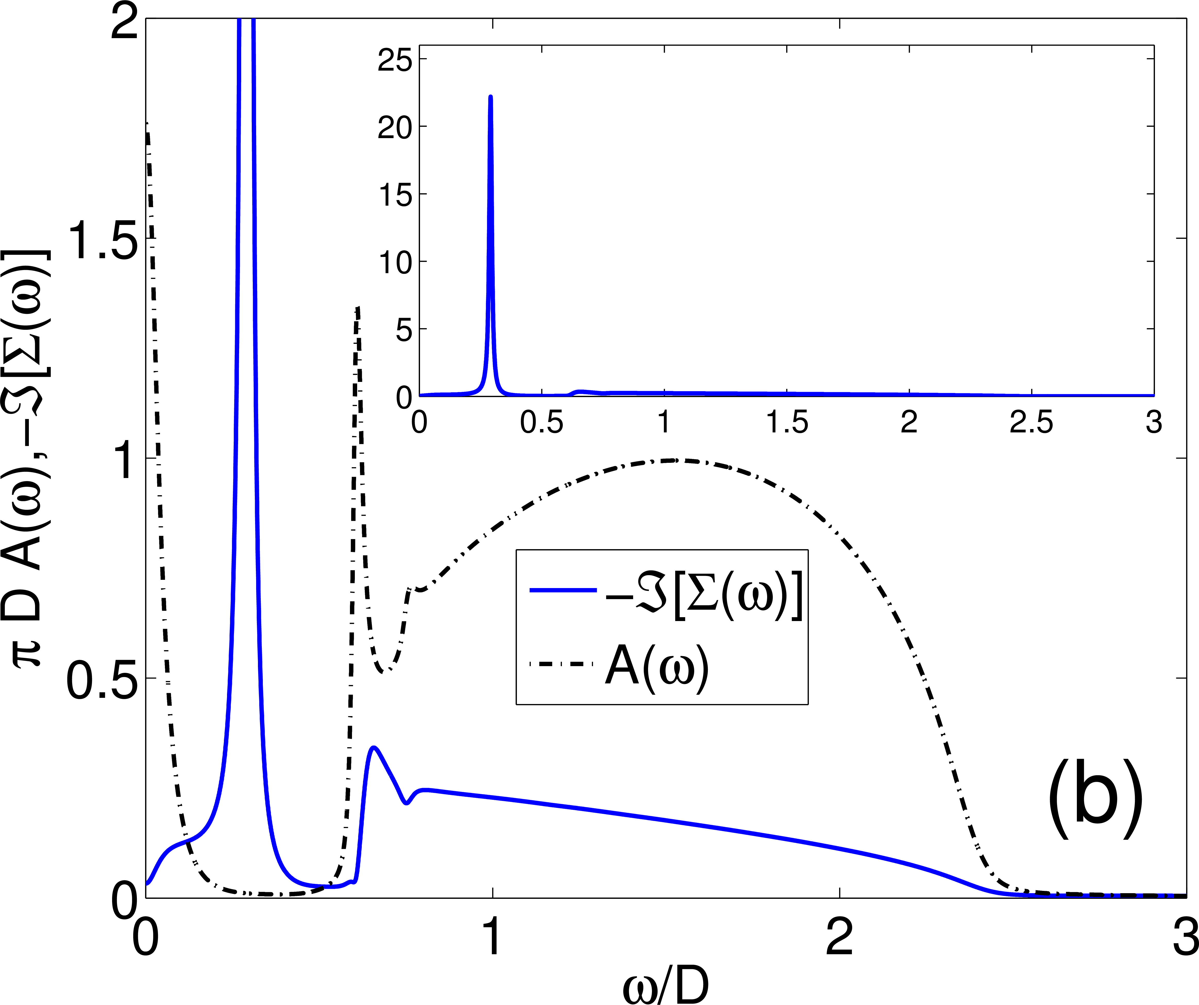
A central object in DMFT is the self energy . Its imaginary part is related to the lifetime of single particle excitations. In Fig. 4 (b) we show the imaginary part of the self energy for . It can be seen clearly that it is small around the position of the sharp side peaks.
IV.3 Time dependencies on the impurity site and connection to side peaks
The appearance of sharp peaks at the inner edge of the Hubbard band has been observed in previous studies in the metallic Ganahl et al. (2014); Lu et al. (2014); Granath and Strand (2012); Karski et al. (2005, 2008) as well as in the insulating phase Granath and Schött (2014); Gull et al. (2010), but has so far eluded a convincing explanation. It has been speculated Karski et al. (2005) to be an anti-bound state of the Fermi-liquid quasi-particle with a collective spin excitation of polaronic character. The existence of collective spin excitations on the other hand requires the presence of spatial correlations, which are not included in single site DMFT. One of the great advantages of our approach is the direct accessibility of time dependent properties of the impurity after the insertion of an electron at . In Fig. 5 we plot the time dependent probabilities (at DMFT self consistency) of finding the impurity in one of the singly occupied states, doubly occupied, , or empty, , with , at and after having inserted a down-electron at at the impurity (for ease of comparison we plot ()). For small we observe a fast decay of the initially high double occupation and a corresponding increase of single occupations. At short times (up to ) we observe strongly damped oscillations corresponding to the Hubbard band, which has a very large imaginary part of the self energy. For times , begins to oscillate at a different frequency . The energy of this oscillations matches the energy of the side-peak at almost perfectly.
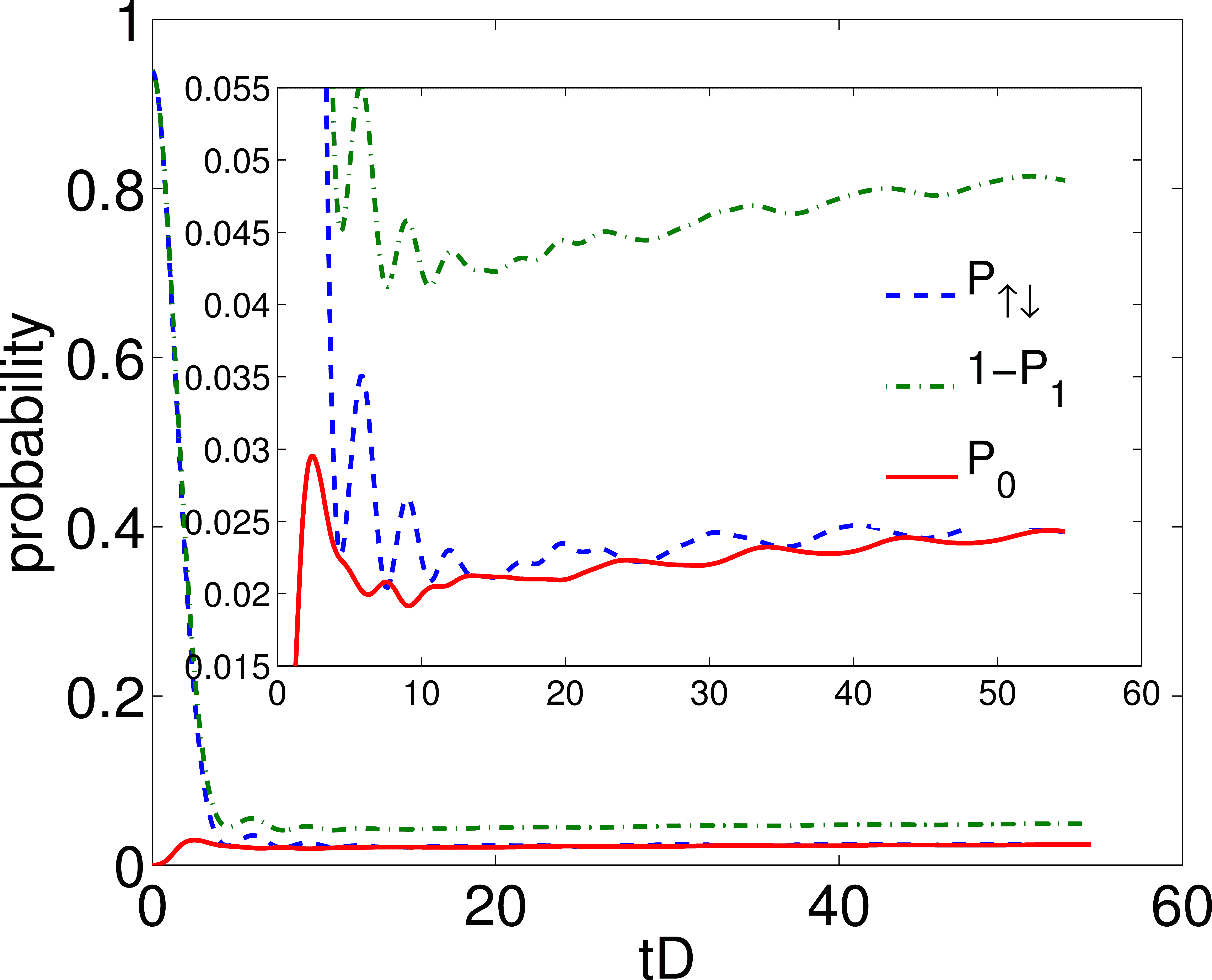
on the other hand rises from exactly 0 to a small finite value, of about the same magnitude as (see Fig. 5) and shows oscillations with the same frequency as but shifted almost exactly by a phase of as compared to . The oscillation in are essentially in phase with those of .
In Fig. 6 we show the time dependence of for different values of and . The inset shows a zoom on the side peak of the corresponding spectral functions . Vertical lines are drawn at the beating frequencies appearing at times . We see that the frequencies of the oscillations closely follow the energies of the Hubbard side peaks. We note that for , where the spectra are almost featureless, the time dependent occupations show no such long-lived oscillations.

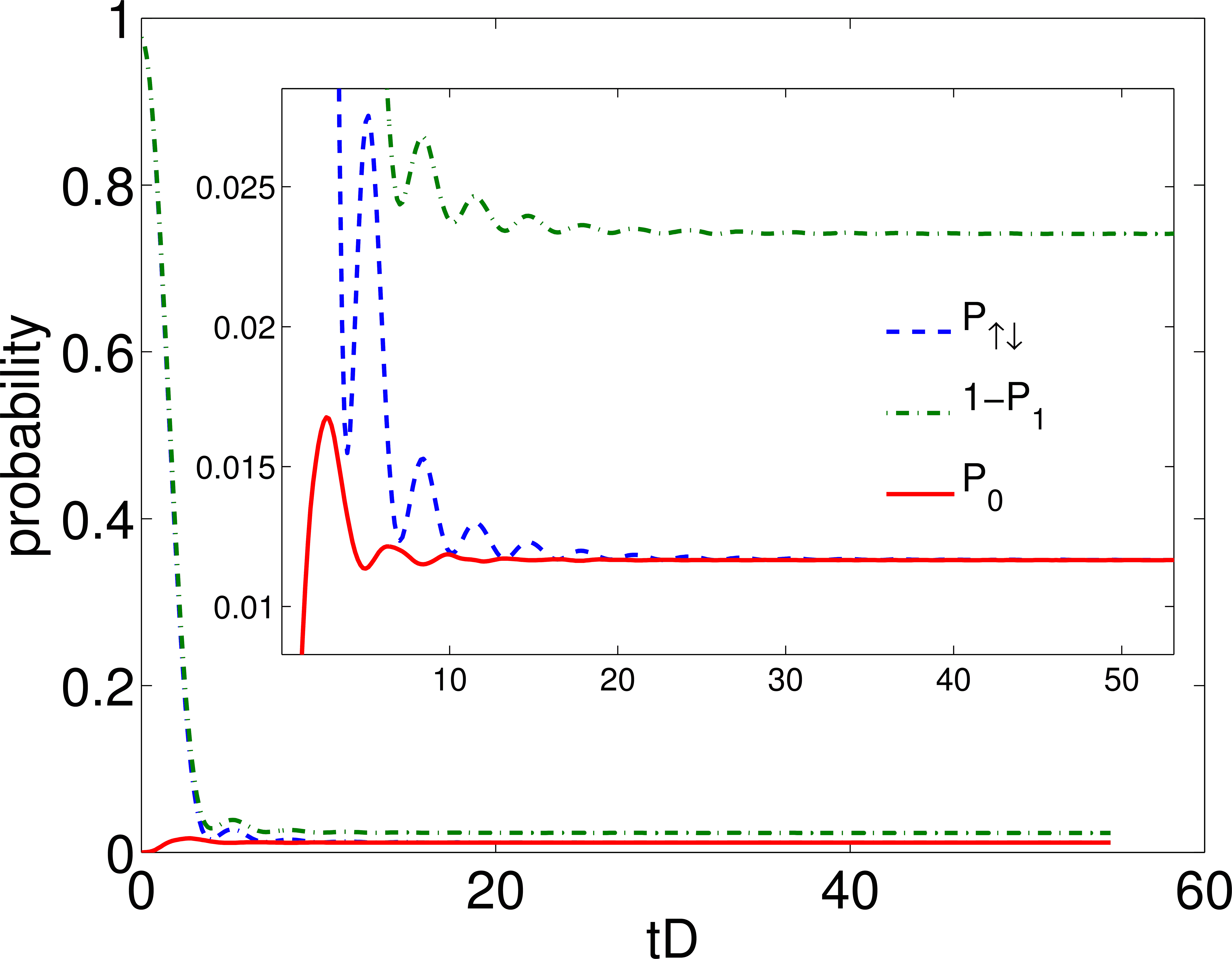
Fig. 7 shows an analysis similar to Fig. 5, but in the insulating phase for . In this case we solely observe oscillations corresponding to the Hubbard bands; a long lived oscillation is not present, which means that in frequency space only the metallic solution has a sharp feature, in agreement with our DMFT spectra above.
Quite generally an oscillation can be associated with a superposition of two eigenstates with an energy difference corresponding to the oscillation frequency. Adding an electron at time to the strongly correlated ground state of the one-band Hubbard model means, if Fourier-transformed to energies, that we will obtain a superposition of eigenstates from all energies. At different energies above the Fermi energy we have three distinct features: the central resonance around , the sharp side-peak at and the broad upper Hubbard band. Unless matrix elements vanish, we will hence have a superposition of states belonging to these energies. Due to the large imaginary part of the self energy of the Hubbard band (see above), this part of the superposition will decohere on short time scales. After this short time, we will remain in a long lived superposition of states belonging to two sharp features, the central Kondo peak and the sharp resonance at the inner side of the Hubbard bands. This leads to the observed oscillations and the frequencies in Figs. 5 and 6.
IV.4 Two-band Hubbard model
Finally, we present results of calculations for the two-band Hubbard model on the Bethe lattice with Hamiltonian Eq. (7). At half-filling this model is know to become a Mott Hubbard insulator, as soon as the interactions are large enough. It is important to note that the Hund coupling is crucial to reach the insulating phase, and increasing lowers the critical value substantially.Georges et al. (2013)
In order to check if our computational parameters in the two-band case allow for the occurence of the sharp features in the Hubbard satellites, we first performed a test using , in which case the two band problem decouples into two independent SIAMs. Indeed, using a value of close enough to the transition we can still resolve the sharp features (not shown), meaning that the accuracy of the method is high enough also for the two band case.
In Fig. 8(a) we now show results for for an interaction strength and Hund’s coupling which is close to the Mott phase Pruschke and Bulla (2005). We compare two different chain lengths and two different Ntm in order to get an estimate of the accuracy of our results. The spectra are almost converged in the system size and show structure within the Hubbard bands.
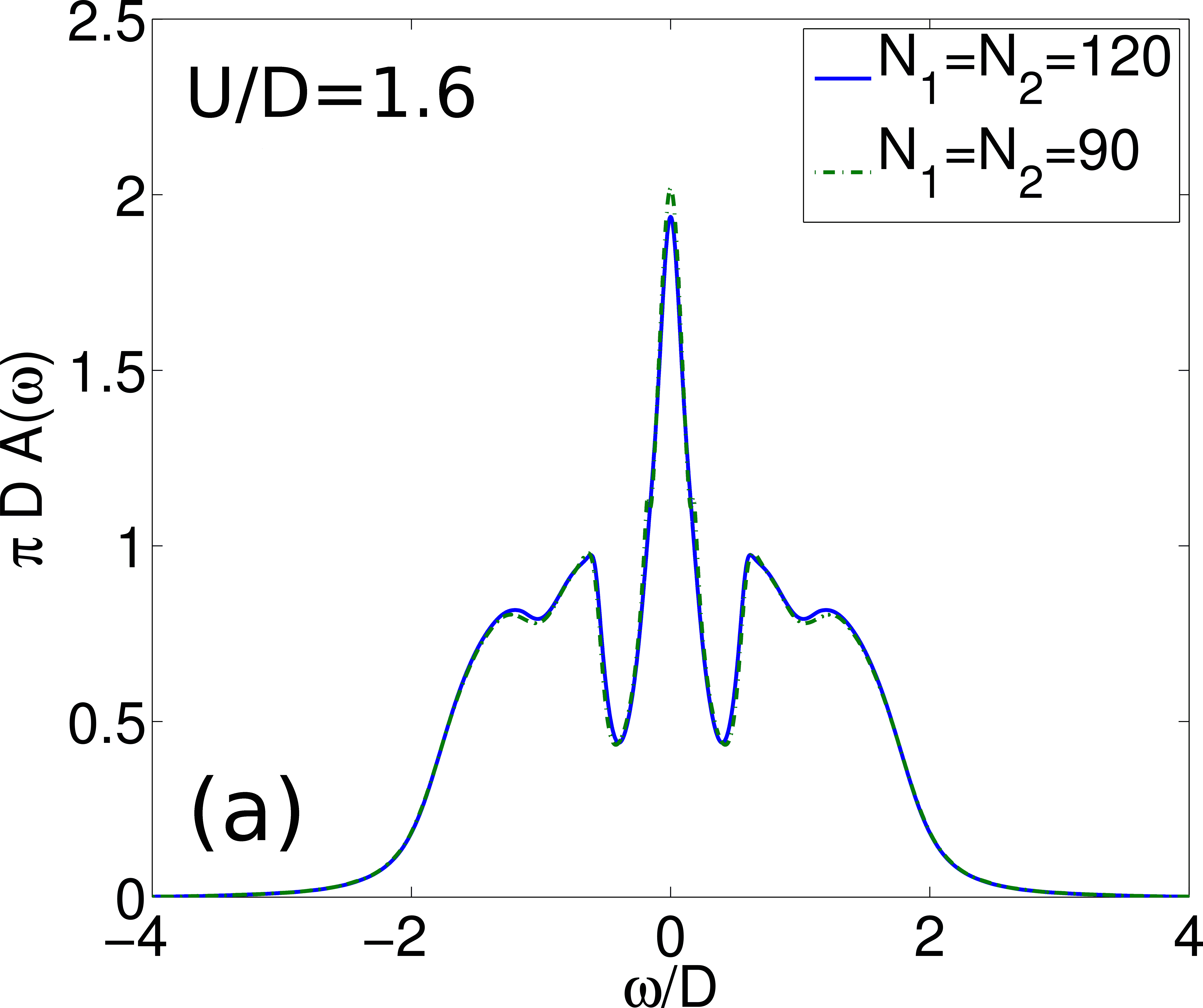
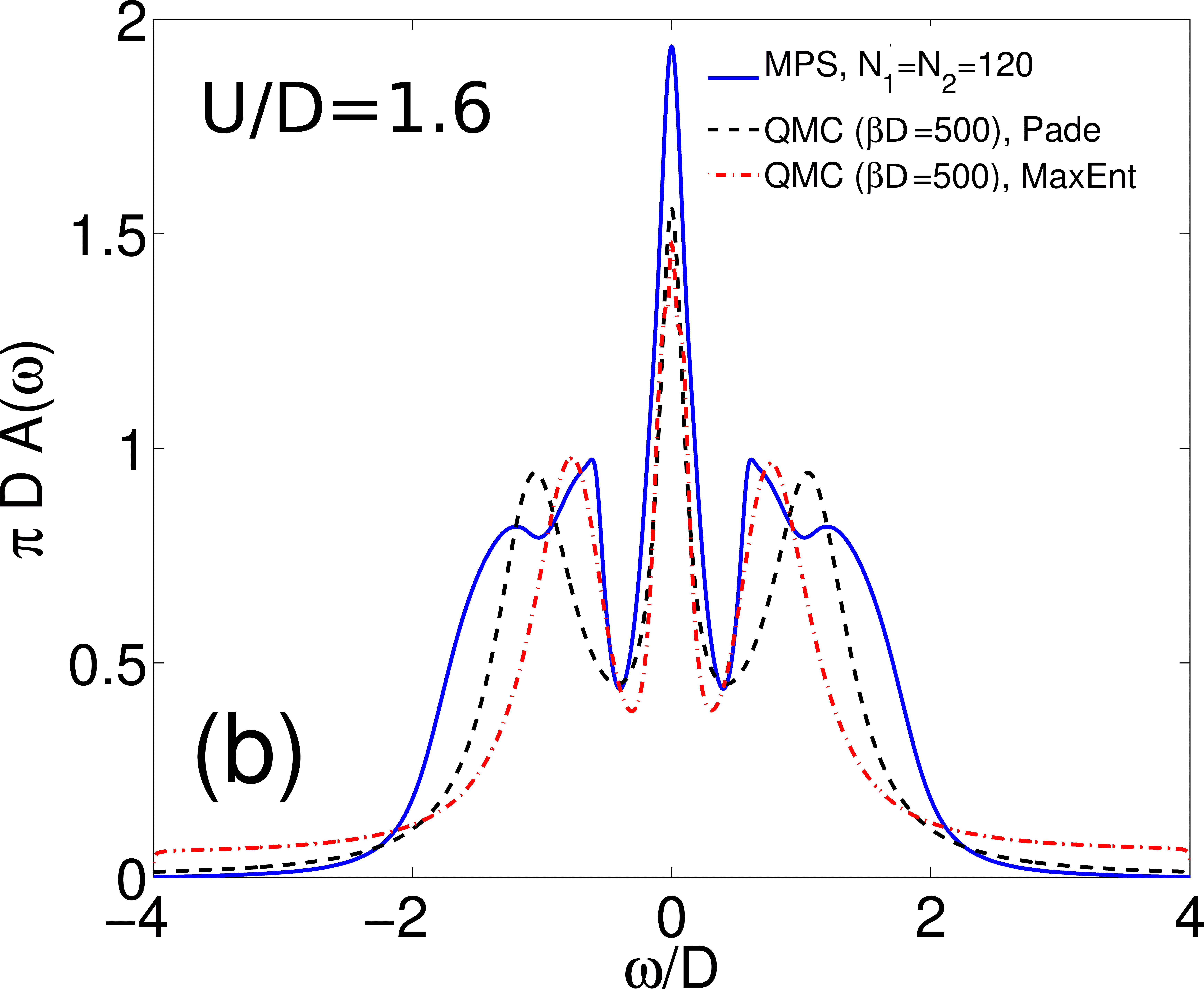
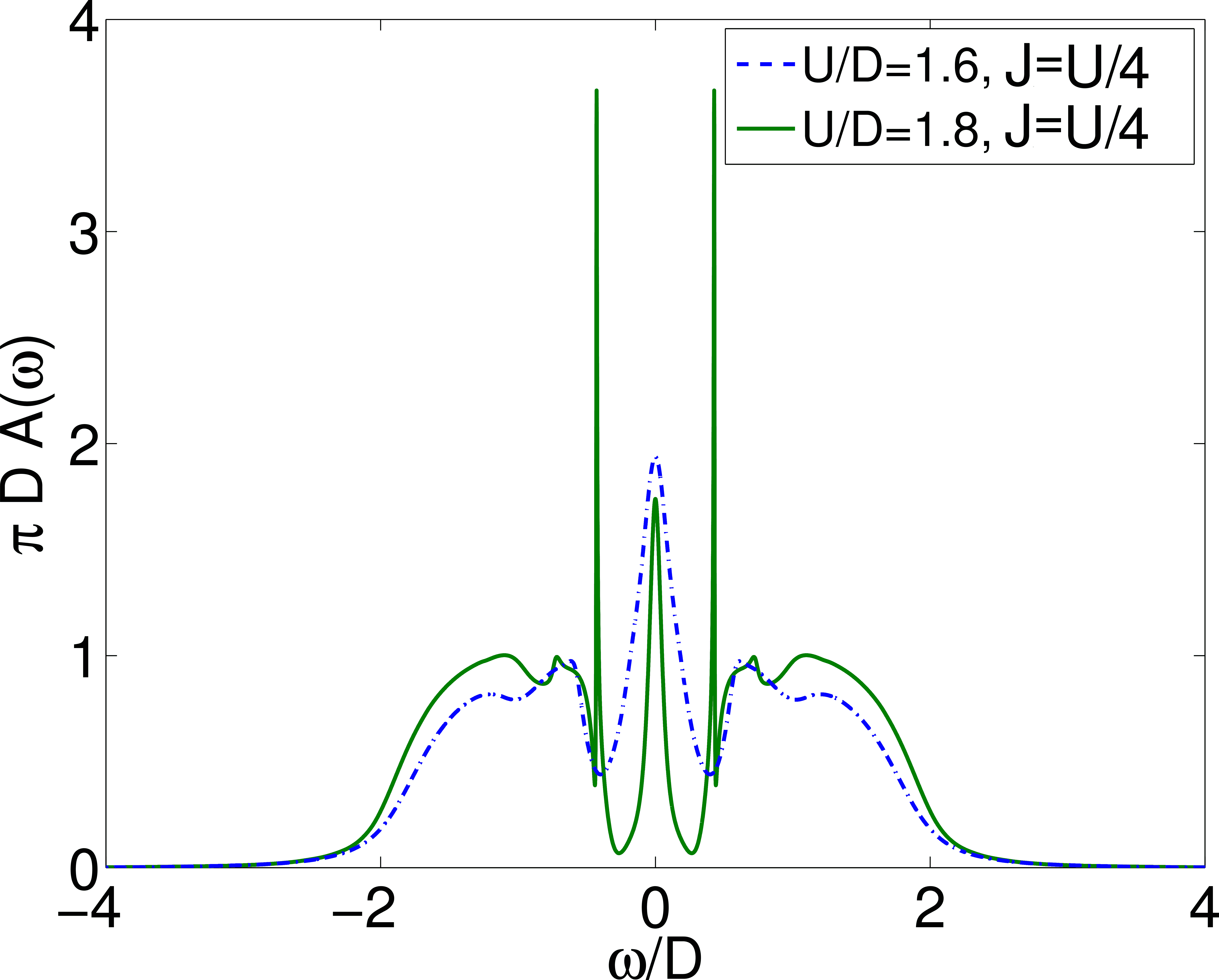
Fig. 8(b) compares our results with ones we obtained using a continuous-time QMC method to solve the two-orbital impurity problem. For the QMC, we employed a hybridization expansion algorithm in matrix form as implemented in the TRIQS package Parcollet et al. (2015); Boehnke et al. (2011); Werner and Millis (2006). This allows us to perform calculations for the full rotationally-invariant Hamiltonian Eq. (7) at low temperatures, . The imaginary-time spectra of QMC have been continued to the real frequency axis using a stochastic Maximum-Entropy method Beach (2004) and alternatively Padé approximants. The qualitative agreement of the position of the Hubbard bands is satisfactory. The features in the Hubbard satellites which are seen in the TEBD results, however, are absent in both analytically continued spectra. (When the separation of these features becomes larger one can, however, resolve the transitions from different atomic states in the analytic continuation Hansmann et al. (2013))
In the atomic limit , a simple analysis shows that the system has only a single one-particle excitation at for two electrons per site. The structure in the Hubbard bands thus originates from admixtures to the ground state with three and one electrons on a site.
In Fig. 9, we plot the spectral function of the two-band Hubbard model for (green solid line), which is already quite close the MI transition. In this case the Hubbard satellites acquire an even richer structure than in the single-band case: as in the latter, we observe the emergence of very sharp features at the inner edges of the Hubbard bands. This suggest that this may be a generic property of the Hubbard model and, to our best knowledge, is the first evidence of these in a multi-orbital Hubbard model. Additionally, at higher energies, we oberve less pronounced features, which are probably related to the Hund’s coupling .
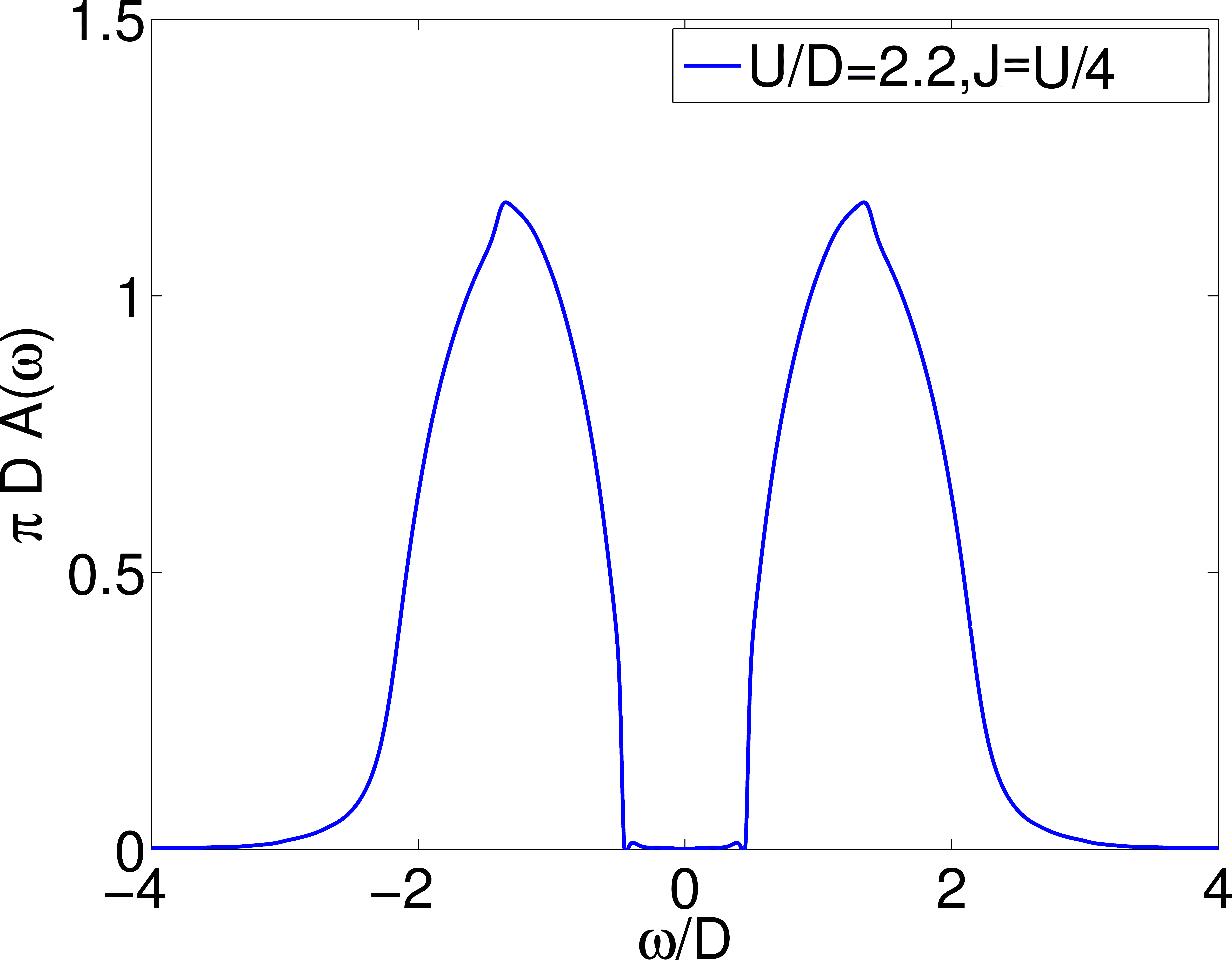
In Fig. 10 we show results for (, see caption for other parameters), which is already in the insulating phase of the system. Substructures in the Hubbard band are visible, though much less pronounced than on the metallic side of the transition. This is in agreement with the fact that the atomic limit of the system shows no splitting (see above). The position of the Hubbard peaks is also already quite well described by the atomic excitations . Importantly, we do not observe any sharp features at the band edges. We note that in this parameter regime calculations are less costly and convergence is much faster than for the metallic case close to the transition.
V Conclusions
We applied the Time Evolving Block Decimation (TEBD) algorithm to construct an impurity solver for dynamical mean-field theory for the single- and two-band Hubbard models on the Bethe lattice. Our method is parallelizable Stoudenmire and White (2013) and scalable to multi-band impurity systems. It works directly at zero temperature and real frequency, without the need for analytic continuation and it produces very accurate results as an impurity solver with high resolution at all frequencies. We applied our method to DMFT for the single-band Hubbard model, where we confirm the existence of a sharp feature at the inner edges of the Hubbard bands. Our results are comparable to the ones obtained in Refs. Karski et al., 2008, 2005, but contrast with ED Lu et al. (2014) and NRG Žitko and Pruschke (2009) results, where this feature is barely present at higher values of . We find a shift of the peak position as a function of . The flexibility and speed of our method allows for accurate parameter studies and real-time dynamics. With respect to the latter we found that adding an electron instantaneously on a lattice results in long-time oscillations of the double, single and zero occupation on this site. We interpret these long-time oscillations as being caused by a superposition of the central Kondo resonance and the sharp side feature in the Hubbard bands. Furthermore, we also applied the method to the two-band Hubbard model on the Bethe lattice. As we approach the phase transition from the metallic side, we observe the developing of rich structures in the Hubbard bands, which are not resolved by our QMC. In particular, we observe the emergence of sharp side peaks, similar to the one-band case. This suggests that these features are a generic property also of multi-orbital Hubbard models close to metal- to Mott-insulator phase transitions. We note that this method is also well suited for applications within non-equilibrium DMFT Wolf et al. (2014) and non-equilibrium master equation approaches Dorda et al. (2015).
Acknowledgements.
The authors acknowledge financial support by the Austrian Science Fund (FWF) through SFB ViCoM F41 projects P03 and P04 (FWF project ID F4103-N13 and F4104-N13) and NAWI Graz. M.G. acknowledges support by the Simons Foundation (Many Electron Collaboration). This research was supported in part by Perimeter Institute for Theoretical Physics. Research at Perimeter Institute is supported by the Government of Canada through Industry Canada and by the Province of Ontario through the Ministry of Economic Development and Innovation. We are grateful for stimulating discussions with S. White, Th. Pruschke and U. Schollwöck. We thank C. Raas for providing his DDMRG data and Jernej Mravlje for providing his Padé code for the QMC data. Simulations were performed at the d-cluster of the TU Graz.VI Appendix
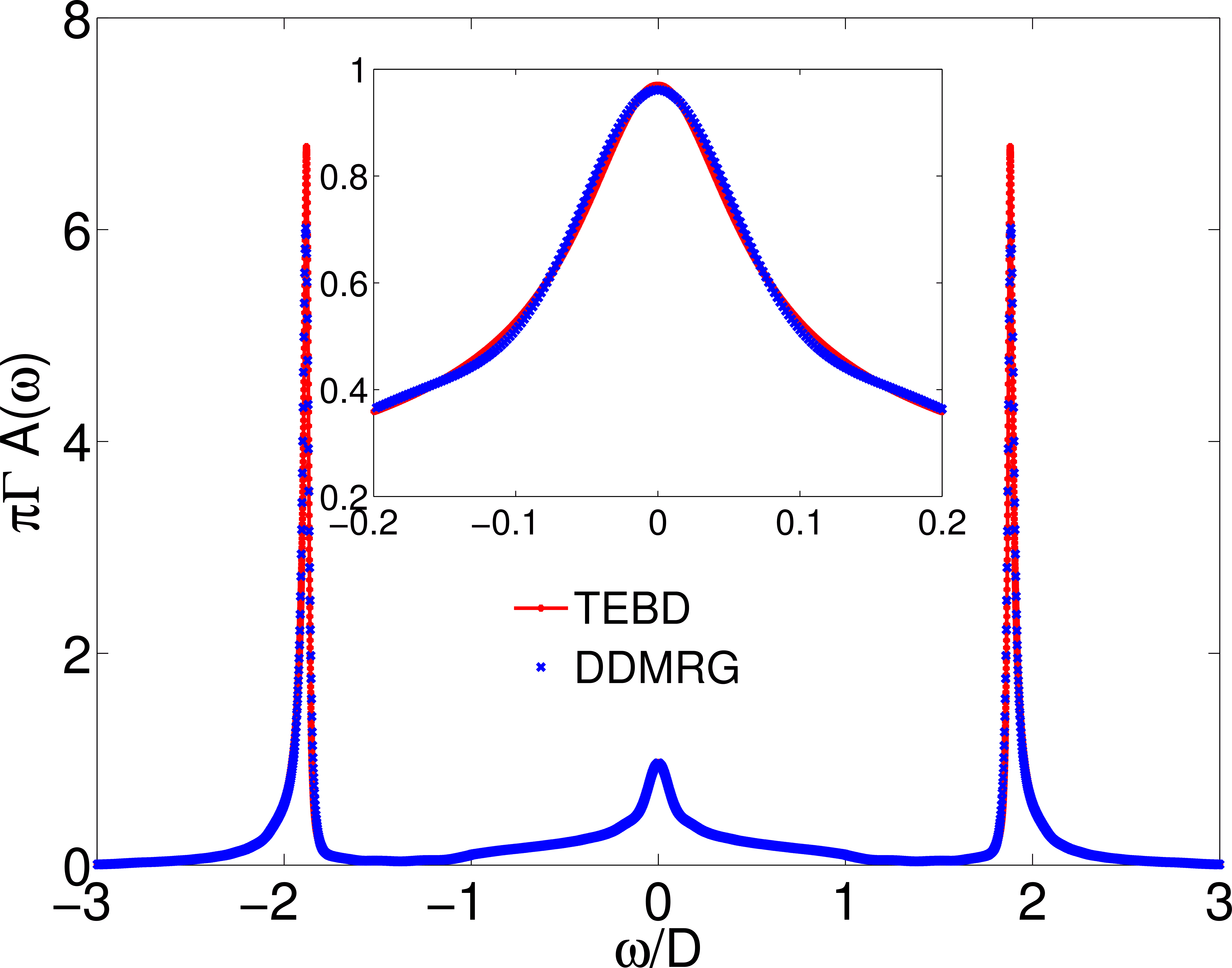


VI.1 Benchmark
We tested the validity and precision of our method as an impurity solver for the case of the single impurity Anderson model at parameters for which results are available from the most precise technique to date, namely the dynamical DMRG Jeckelmann (2002); Karski et al. (2008, 2005); Ganahl et al. (2014). We used a semi-circular bath DOS and a hybridization strength (corresponding to a uniform hybridization ) Bulla et al. (2008), at an interaction strength of . Spectra are found in Fig. A1. We note that DDMRG involves separate calculations at each frequency and a deconvolution of the resulting spectra. The agreement is almost perfect.
VI.2 Parameter studies for prediction
Here we present more detailed results on the influence of the prediction parameters and the number of measured data points . In Fig. A2 we show a DMFT-spectrum with and large eigenvalues normalized to unity (black solid line). It is instructive to take these converged results and from the data of the last iteration calculate the spectral function with different pseudo-inverse cutoffs and different treatment of large eigenvalues. We see that setting eigenvalues to unity tends to produce an overshoot at , whereas results with zeroed eigenvalues are stable and converged at . This behavior remains the same when doing full DMFT cycles. For eigenvalues rescaled to unity we also observe that for small the prediction can pick up errors due to truncation and Trotter breakup, leading to artificial structures in the spectral functions. We conclude that converged results can best be obtained by setting large eigenvalues to zero and choosing .
In Fig. A3 we analyze the effect of on the fixed point of the DMFT iterations for and . We take , large enough to use different without getting reflections from the boundaries of the system, which would spoil the linear prediction. We observe a very slight non-monotonic behavior of the Hubbard side peak height as well as the peak position (left inset). The quasi particle peak height shows the same non-monotonic behavior (right inset). We attribute this behavior to truncation and Trotter effects, which become stronger for increasing , also confirmed by tiny artificial structures in the pseudo-gap region for . The dependence of the fixed point on is very small. Using a large does not improve systematically on the results, hence for computational efficiency we use in the main paper.
VI.3 Time dependence of
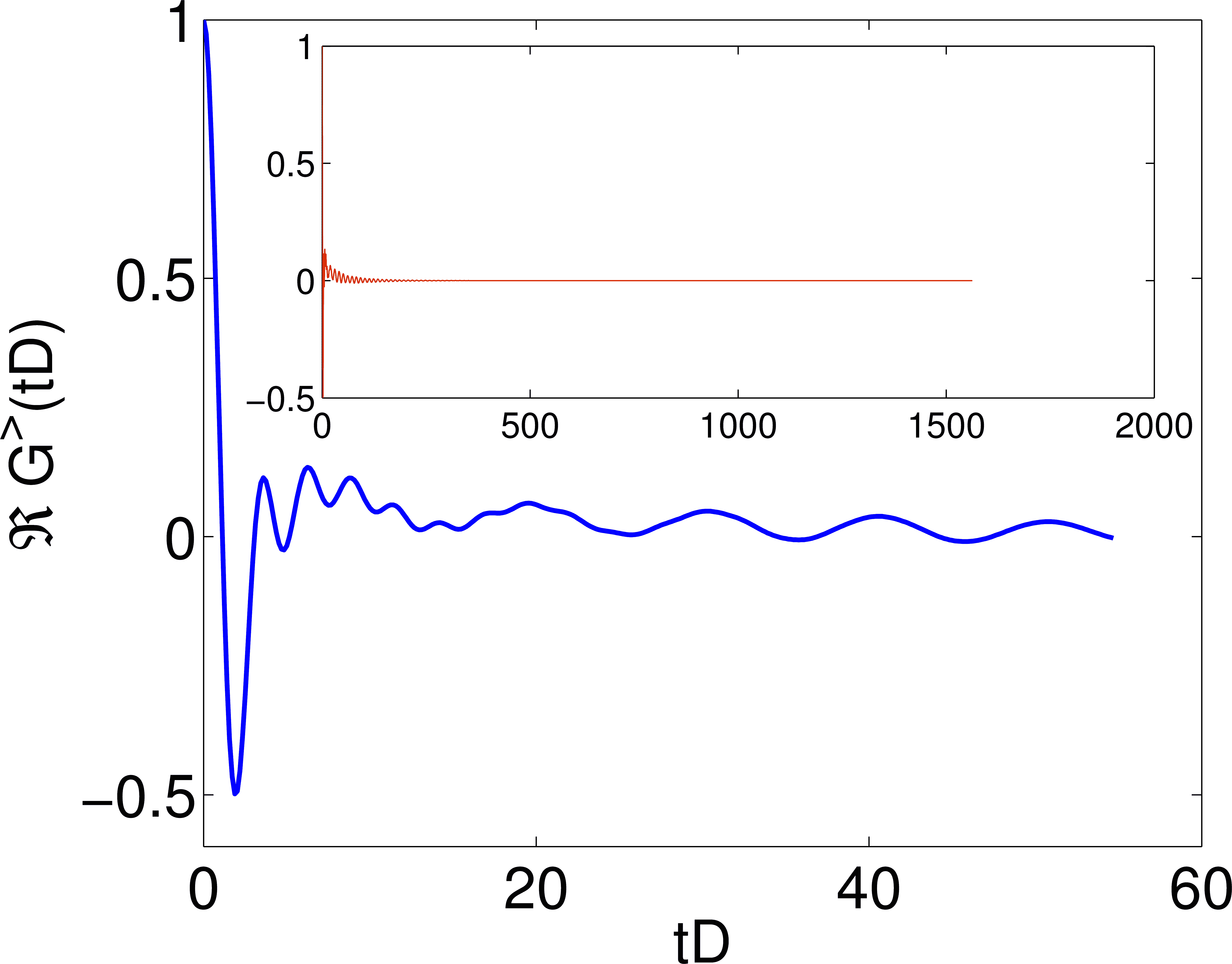
We complement the time-dependent analysis of local observables by showing the evolution of the time-dependent Greens function, from which the spectral function is obtained by Fourier transformation to the frequency domain. In Fig. A4 we show the time dependence of the bigger Greens function for (parameters the same as in Fig. 4)). The main figure shows the MPS results which nicely display the beating related to the side peak in the Hubbard bands. The inset shows the timeseries obtained from linear prediction, all the way to the long time limit used in the Fourier transformation.
References
- Kondo (1964) J. Kondo, Progress of Theoretical Physics 32, 37 (1964).
- Wilson (1975) K. G. Wilson, Rev. Mod. Phys. 47, 773 (1975).
- Kouwenhoven and Glazman (2001) L. Kouwenhoven and L. Glazman, Phys. World 14 (1), 33 (2001).
- Metzner and Vollhardt (1989) W. Metzner and D. Vollhardt, Phys. Rev. Lett. 62, 324 (1989).
- Georges et al. (1996) A. Georges, G. Kotliar, W. Krauth, and M. J. Rozenberg, Rev. Mod. Phys. 68, 13 (1996).
- Georges (2004) A. Georges, arXiv:cond-mat/0403123 (2004).
- Assaad and Evertz (2008) F. F. Assaad and H. G. Evertz, in Computational Many-Particle Physics (Springer Berlin Heidelberg, 2008), 739, pp. 277–356.
- Gull et al. (2011) E. Gull, A. J. Millis, A. I. Lichtenstein, A. N. Rubtsov, M. Troyer, and P. Werner, Rev. Mod. Phys. 83, 349 (2011).
- Bulla et al. (2008) R. Bulla, T. A. Costi, and T. Pruschke, Rev. Mod. Phys. 80, 395 (2008).
- White (1992) S. R. White, Phys. Rev. Lett. 69, 2863 (1992).
- White (1993) S. R. White, Phys. Rev. B 48, 10345 (1993).
- Schollwöck (2011) U. Schollwöck, Ann. Phys. 326, 96 (2011).
- Sénéchal et al. (2000) D. Sénéchal, D. Perez, and M. Pioro-Ladriére, Physical Review Letters 84, 522 (2000).
- Potthoff et al. (2003) M. Potthoff, M. Aichhorn, and C. Dahnken, Physical Review Letters 91, 206402 (2003).
- Jarrell (1992) M. Jarrell, Phys. Rev. Lett. 69, 168 (1992).
- Rozenberg et al. (1992) M. J. Rozenberg, X. Y. Zhang, and G. Kotliar, Phys. Rev. Lett. 69, 1236 (1992).
- Parcollet et al. (2015) O. Parcollet, M. Ferrero, T. Ayral, H. Hafermann, I. Krivenko, L. Messio, and P. Seth, arXiv:1504.01952 (2015), URL http://arxiv.org/abs/1504.01952.
- Boehnke et al. (2011) L. Boehnke, H. Hafermann, M. Ferrero, F. Lechermann, and O. Parcollet, Phys. Rev. B 84, 075145 (2011).
- Parragh et al. (2012) N. Parragh, A. Toschi, K. Held, and G. Sangiovanni, Phys. Rev. B 86, 155158 (2012).
- Caffarel and Krauth (1994) M. Caffarel and W. Krauth, Phys. Rev. Lett. 72, 1545 (1994).
- Sangiovanni et al. (2006) G. Sangiovanni, A. Toschi, E. Koch, K. Held, M. Capone, C. Castellani, O. Gunnarsson, S.-K. Mo, J. W. Allen, H.-D. Kim, et al., Phys. Rev. B 73, 205121 (2006).
- Granath and Strand (2012) M. Granath and H. U. R. Strand, Phys. Rev. B 86, 115111 (2012).
- Lu et al. (2014) Y. Lu, M. Höppner, O. Gunnarsson, and M. W. Haverkort, Physical Review B 90, 085102 (2014), URL http://link.aps.org/doi/10.1103/PhysRevB.90.085102.
- Žitko and Pruschke (2009) R. Žitko and T. Pruschke, Phys. Rev. B 79, 085106 (2009).
- Pruschke and Bulla (2005) T. Pruschke and R. Bulla, Eur. Phys. J. B 44, 217 (2005).
- Bulla (1999) R. Bulla, Phys. Rev. Lett. 83, 136 (1999).
- Mühlbacher and Rabani (2008) L. Mühlbacher and E. Rabani, Physical Review Letters 100, 176403 (2008).
- Werner et al. (2009) P. Werner, T. Oka, and A. J. Millis, Physical Review B 79, 035320 (2009).
- Prokof’ev and Svistunov (2007) N. Prokof’ev and B. Svistunov, Physical Review Letters 99, 250201 (2007).
- Gull et al. (2010) E. Gull, D. R. Reichman, and A. J. Millis, Phys. Rev. B 82, 075109 (2010).
- Cohen et al. (2014a) G. Cohen, E. Gull, D. R. Reichman, and A. J. Millis, Phys. Rev. Lett. 112, 146802 (2014a).
- Cohen et al. (2014b) G. Cohen, D. R. Reichman, A. J. Millis, and E. Gull, Phy. Rev. B 89, 115139 (2014b).
- Granath and Schött (2014) M. Granath and J. Schött, Physical Review B 90, 235129 (2014), URL http://link.aps.org/doi/10.1103/PhysRevB.90.235129.
- Greger et al. (2013) M. Greger, M. Kollar, and D. Vollhardt, Phys. Rev. Lett. 110, 046403 (2013).
- Jeckelmann (2002) E. Jeckelmann, Phys. Rev. B 66, 045114 (2002).
- Kühner and White (1999) T. D. Kühner and S. R. White, Phys. Rev. B 60, 335 (1999).
- Peters (2011) R. Peters, Phys. Rev. B 84, 075139 (2011).
- Karski et al. (2008) M. Karski, C. Raas, and G. S. Uhrig, Phys. Rev. B 77, 075116 (2008).
- Karski et al. (2005) M. Karski, C. Raas, and G. S. Uhrig, Phys. Rev. B 72, 113110 (2005).
- Nishimoto et al. (2004) S. Nishimoto, F. Gebhard, and E. Jeckelmann, J. Phys.: Condens. Matter 16, 7063 (2004).
- García et al. (2004) D. J. García, K. Hallberg, and M. J. Rozenberg, Phys. Rev. Lett. 93, 246403 (2004).
- Hallberg (1995) K. A. Hallberg, Phys. Rev. B 52, R9827 (1995).
- Holzner et al. (2011) A. Holzner, A. Weichselbaum, I. P. McCulloch, U. Schollwöck, and J. von Delft, Phys. Rev. B 83, 195115 (2011).
- Weiße et al. (2006) A. Weiße, G. Wellein, A. Alvermann, and H. Fehske, Rev. Mod. Phys. 78, 275 (2006).
- Ganahl et al. (2014) M. Ganahl, P. Thunström, F. Verstraete, K. Held, and H. G. Evertz, Phys. Rev. B 90, 045144 (2014).
- Vidal (2004) G. Vidal, Phys. Rev. Lett. 93, 040502 (2004).
- Vidal (2003) G. Vidal, Phys. Rev. Lett. 91, 147902 (2003).
- Verstraete et al. (2008) F. Verstraete, V. Murg, and J. Cirac, Adv. Phys. 57, 143 (2008).
- White and Affleck (2008) S. R. White and I. Affleck, Phys. Rev. B 77, 134437 (2008).
- Barthel et al. (2009) T. Barthel, U. Schollwöck, and S. R. White, Phys. Rev. B 79, 245101 (2009).
- Wolf et al. (2015) F. A. Wolf, J. A. Justiniano, I. P. McCulloch, and U. Schollwöck, Phys. Rev. B 91, 115144 (2015).
- Koga et al. (2002) A. Koga, Y. Imai, and N. Kawakami, Phys. Rev. B 66, 165107 (2002).
- Han et al. (1998) J. E. Han, M. Jarrell, and D. L. Cox, Phys. Rev. B 58, R4199 (1998).
- Held and Vollhardt (1998) K. Held and D. Vollhardt, Eur. Phys. J. B 5, 473 (1998).
- Barthel (2013) T. Barthel, New J. Phys. 15, 073010 (2013).
- Saberi et al. (2008) H. Saberi, A. Weichselbaum, and J. von Delft, Phys. Rev. B 78, 035124 (2008).
- Holzner et al. (2010) A. Holzner, A. Weichselbaum, and J. von Delft, Phys. Rev. B 81, 125126 (2010).
- Press et al. (2007) W. H. Press, S. A. Teukolsky, W. T. Vetterling, and B. P. Flannery, Numerical Recipes in C, 3rd edition (Cambridge University Press, 2007).
- Raas and Uhrig (2005) C. Raas and G. S. Uhrig, Eur. Phys. J. B 45, 293 (2005).
- Hewson (1993) A. C. Hewson, The Kondo Problem to Heavy Fermions (Cambridge University Press, 1993).
- Georges et al. (2013) A. Georges, L. d. Medici, and J. Mravlje, Annual Review of Condensed Matter Physics 4, 137 (2013).
- (62) In the one-band case, and correspond to total simulated times of and , resp.; in the two-band case, and correspond to and .
- Werner and Millis (2006) P. Werner and A. J. Millis, Phys. Rev. B 74, 155107 (2006).
- Beach (2004) K. S. D. Beach, arXiv:cond-mat/0403055 (2004).
- Hansmann et al. (2013) P. Hansmann, A. Toschi, G. Sangiovanni, T. Saha-Dasgupta, S. Lupi, M. Marsi, and K. Held, Phys. Status Solidi 250, 1251 (2013).
- Stoudenmire and White (2013) E. M. Stoudenmire and S. R. White, Phys. Rev. B 87, 155137 (2013).
- Wolf et al. (2014) F. A. Wolf, I. P. McCulloch, and U. Schollwöck, Phys. Rev. B 90, 235131 (2014).
- Dorda et al. (2015) A. Dorda, M. Ganahl, H. G. Evertz, W. von der Linden, and E. Arrigoni, arXiv:cond-mat/1507.02982 (2015).