Reanalyzing the upper limit on the tensor-to-scalar perturbation ratio in a quartic potential inflationary model
Abstract
We study the polynomial chaotic inflation model with a single scalar field in a double well quartic potential which has recently been shown to be consistent with Planck data. In particular, we study the effects of lifting the degeneracy between the two vacua on the inflationary observables, i.e., spectral index and tensor-to-scalar perturbation ratio . We find that removing the degeneracy allows the model to satisfy the upper limit constraints on from Planck data, provided the field starts near the local maximum. We also calculate the scalar power spectrum and non-Gaussianity parameter for the primordial scalar perturbations in this model.
1 Introduction
Inflation is regarded as the standard cosmological paradigm to describe the physics of the very early Universe. It leads to a causal mechanism to generate almost scale invariant fluctuations on cosmological scales, with small deviations that follow from the precise microphysics of inflation. This prediction is consistent with the recently announced measurements of the cosmic microwave background (CMB) anisotropies by the Planck satellite. The latest data allow us to constrain the inflationary model besides giving a slightly red tilted spectral index = 0.9603 0.0073, ruling out exact scale invariance = 1 at over 5 [1]. The Planck data also provide observational bounds on primordial non-Gaussianity parameter, i.e., local at 68% confidence level for the reduced bispectrum [2].
Just after Planck results were announced, different scalar potentials were revisited to explore concordance with these results [1]. The data reinforced the ruling out of single-field inflationary models with , which were already disfavored or marginally disfavored by WMAP. (This does not apply to alternative inflationary scenarios e.g., warm inflation [3]). However Croon et al. [4] demonstrated that the double well degenerate potential is consistent with Planck data, although with severe constraints on the initial condition for and on the allowed range of . The polynomial quartic potential with double well is the most studied potential in a variety of settings. It is also well motivated by the physics beyond the Standard Model, viz. supergravity and superstring theories [5]. The characteristic interesting features [4, 6] of the potential have been the primary motivation for a lot of effort to explore its consistency with the Planck data [1].
2 Basic Formalism
2.1 Slow Roll Parameters
We review the formalism in [4] to set up our notation. For an inflationary model described by the potential , the slow-roll parameters are defined as
| (1) |
| (2) |
and
| (3) | ||||
where
| (4) |
In terms of the slow-roll parameters, the scalar spectral index is expressed as
| (5) |
and the tensor-to-scalar ratio as
| (6) |
Finally the number of e-folds is given by
| (7) |
where are the values of at the end and beginning of the inflationary epoch.
The scalar power spectrum is described in terms of the spectral index by
| (8) |
where
| (9) |
which in terms of slow-roll parameters is
| (10) |
2.2 Inflaton Potential and Background Dynamics
On parameterizing the field as , where is dimensionless, for the chosen potential in [4], the inflationary observables reduce to111In [4], a minus sign is missing in the expression for . Further, the power of in their Eq.(10), generalised in our Eq.(13), should be 4 and not 2. This error creeps into the numerical calculation (in table) also. A summary of standard formulae can be found in [7].:
| (11) |
| (12) |
| (13) |
and
| (14) |
We point out that the range of possible initial field values is severely restricted if , as the integral for will not converge on choosing an initial field value beyond the local maximum (see Fig. 6). This rules out the possibility of investigation of deviation from slow-roll or multiphase-inflation. Punctuated inflation [6] is the simplest and interesting example of multi-phase-inflation which occurs in our model when and the initial field value is chosen beyond the point of inflection.
We now explore the behavior of the inflationary observables, including and as is varied from 1 to 0 within the slow-roll regime. Our analysis suggests a broad range of for which prediction in the plane lies within the 1 level.
2.3 Discussion about the potential shape
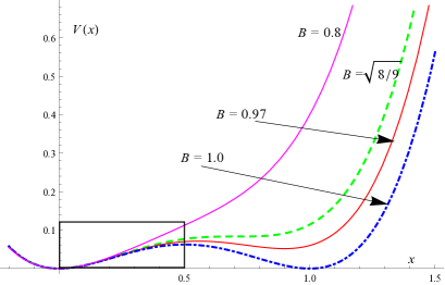
The global shape of the potential depends on the coefficient as shown in Fig. 1. For , there is one local maximum at and two degenerate minima at and 1.0. For , the minimum at is lifted. As long as there is such a local maximum, the initial value of the inflaton field should be below the local maximum since otherwise the inflaton would be trapped in the false vacuum.
The false vacuum disappears for . Interestingly, if marginally satisfies the inequality, there appears a flat plateau at around the point of inflection. If one starts at a suitable value of the field beyond the point of inflection in the above potential, it is found that one can achieve two epochs of slow roll inflation sandwiching a brief period of departure from inflation (lasting for a little less than one e-fold ), a scenario which has been dubbed as punctuated inflation [6]. In fact, it is the point of inflection, around which the potential exhibits a plateau with an extremely small curvature, which permits such an evolution to be possible.
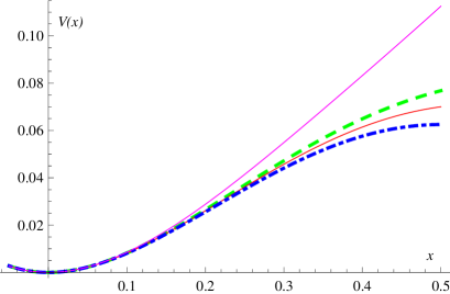
It needs to be kept in mind that this potential does not provide a single inflation model, but rather a class of the inflationary models as we vary from 0 to 1. Fig. 1 describes the potential profile for four values of . Interestingly, there are two ways to mimic the quadratic potential case: (a) by changing the class of potential by decreasing from 1 to 0 and (b) by taking the initial field value very near to zero (near the first minimum) [4]. However, as shown in Fig. 1b, each member of the class is asymptotic to the quadratic case if irrespective of the value of .
3 Numerical Results
We set out to explore the model for the entire range of values from 0 to 1 and for an arbitrary initial field value (or equivalently ). We need to keep in mind that an arbitrary large initial field value can be taken only for those members of the class for which , otherwise either deviation from slow roll will occur (when ) or the field will be trapped in the false vacuum (when ).
3.1 Prediction in plane
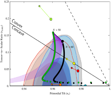
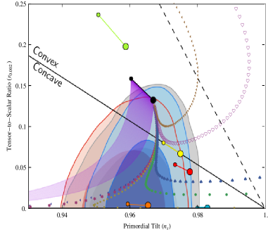
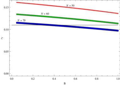
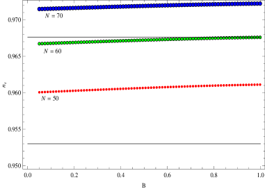
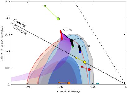
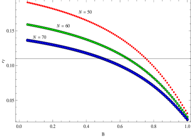
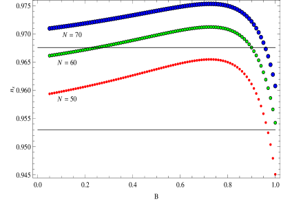
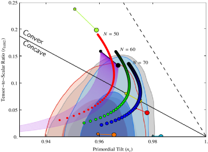
Fig. 3 exhibits how our analysis differs from the past work of Nakayama et al. [5] (see Fig. 2), where effects mainly due to varying initial field value are considered. In contrast, we have varied continuously for each fixed initial field value—from the one near the minimum at to the other near the local maximum—and for three e-fold values: N = 50, 60 and 70. However, we have shown the analysis only for the two extreme initial field values because of clarity and reasons of space (see Figs. 3 and 4).
Plots only on the plane, as done in [5], hide valuable information of initial conditions for which the model lies within 1. Notice that very near to , predictions (i.e., points in the plane) start from the quadratic potential (the black line), found concordant with the Planck data, and then graze the contour as is increased; see Figs. 2 and 7.
From Fig. 3a, it is clear that for = 50 (red) and 60 (green), this model is completely above the bound imposed by Planck () for the entire range of —here the field starts near the origin; whereas for = 70 (blue), the model is at the margin of this bound.
When we contrast the above situation with Fig. 4a, we find that the upper limit on is satisfied for sufficiently large values of (red and green curves fall below the horizontal line for and respectively). It is emphasized that this is the case when the field starts near the local maximum (). Fig. 4c makes this explicit, showing that even a part of the red curve ( = 50) is within 1 of the Planck value. Although there is no appreciable disagreement between Planck and BICEP2 results as clarified in [8], a slightly larger tensor-to-scalar ratio , as required by BICEP2, is within reach (e.g., when ) as shown in Fig. 4a. Another way to realize a large is by assuming the non-monotonicity of the slow-roll parameter , as considered in a model somewhat similar to ours [9].
3.2 Non-Gaussianity
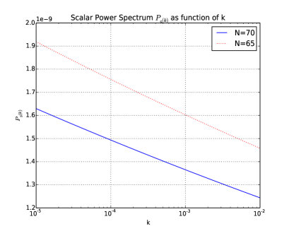
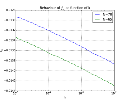
Non-Gaussianity is now a standard cosmological observable, comparable to the spectral index () and tensor-to-scalar ratio , and is a powerful discriminant between competing models. It is therefore desirable to study aspects of non-Gaussianity for this model too. We have numerically calculated the equilateral limit of the local parameter [10]. In Fig. 5a, the power spectrum is plotted as a function of , from which it is clear that the spectrum is not scale invariant on any scale (otherwise it would have been a horizontal straight line). In Fig. 5b, the non-Gaussianity parameter are plotted as a function of , from which we observe that the very low values of lie in the range predicted by Planck data for local = 2.7 5.8 [2]. The very small non-Gaussianity, inferred from BICEP2 data owing to comparatively larger [11] (see also [12]), is compatible with our results also [13]. This observation is also consistent with the fact that single-field slow roll models predict a very small non-Gaussianity [14].
4 Summary and Conclusion
In this Letter, we have explored in detail the space within the slow-roll regime for the quartic potential. We have explicitly shown that on varying , interesting patterns on the variation of and arise only when field dynamics captures the deviation from the quadratic case, i.e., the field should start near the local maximum, not near the origin. Even though this parameter space has been moderately studied in [5], the authors restricted their analysis to a few discrete values of . Similarly Ellis et al. [15] have carried out a statistical study with just four explicit values of numerical coefficient in a two field model to explore concordance with the preferred observational values of and .
One of the main well-known problems—constraints from Planck on the upper limit on —has been reanalyzed here and we find that there is no respite for the model solely due to removing degeneracy between the vacua. On the other hand, merging variations of with the field starting near the local maximum, the model’s predictions for lie well within 1 for a large part of the space (see Fig. 4). Further, our Fig. 4a clearly shows that large can be generated when the potential is non-degenerate and the field starts near the local maximum. On non-Gaussianity aspects ( which were not considered in previous works [4],[5]), we have explicitly calculated the local parameter for each mode of our interest and verified that this model indeed satisfies the constraint imposed by Planck data on non-Gaussianity [2], and is compatible with BICEP2 measurements.
Acknowledgments
RK thanks Dheeraj Kumar Hazra for useful communication and Tarun Choudhari for assistance with Latex. We are grateful to Rudnei O. Ramos and Sayantan Choudhury for pointing out their works [3] and [9, 12] respectively. We also thank an anonymous reviewer whose comments helped us highlight the subtle points of our study. The work of RK was partially supported by CSIR, New Delhi with the award of JRF (No. 09/045(0930)/2010-EMR-I).
Appendix
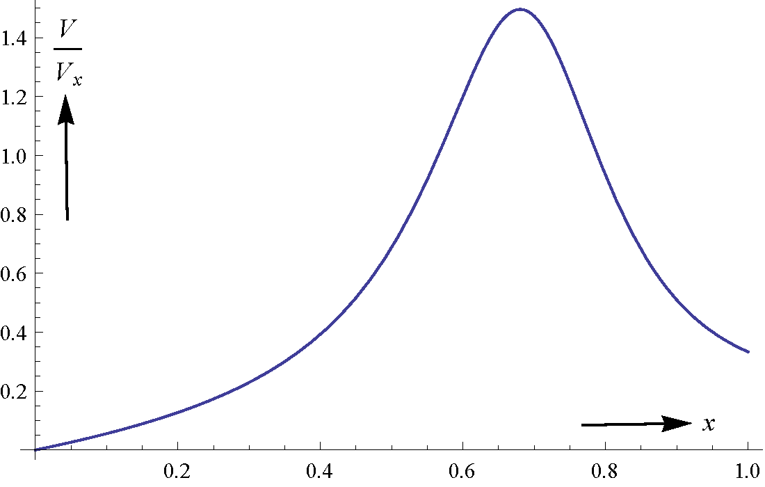
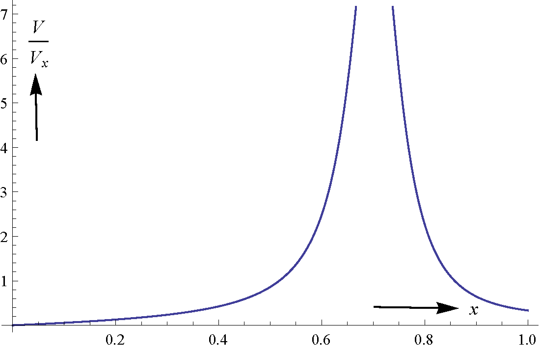
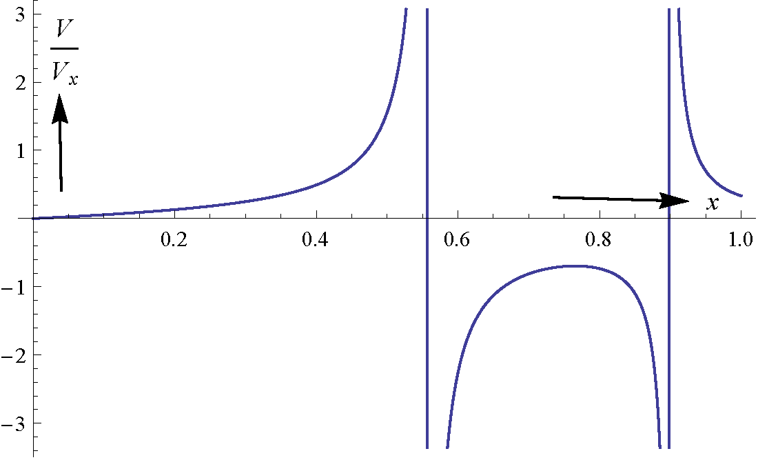
In Fig. 6, we plot the integrand for for 3 values of . (As already mentioned, one minimum disappears if .) We can clearly see how a discontinuity in develops as increases above . One cannot take any point on the axis beyond the local maximum, which is near with a slight variation as we change (see Fig. 1).
References
References
- [1] P. Collaboration, P. A. R. Ade, Planck 2013 results. XXII. Constraints on inflation arXiv:1303.5082.
-
[2]
P. Collaboration, P. A. R. Ade, Planck
2013 results. XXIV. constraints on primordial non-gaussianity,
arXiv:1303.5084 [astro-ph].
URL http://arxiv.org/abs/1303.5084 -
[3]
R. O. Ramos, L. A. da Silva, Power
spectrum for inflation models with quantum and thermal noises, Journal of
Cosmology and Astroparticle Physics 2013 (03) (2013) 032–032, arXiv:
1302.3544.
doi:10.1088/1475-7516/2013/03/032.
URL http://arxiv.org/abs/1302.3544 -
[4]
D. Croon, J. Ellis, N. E. Mavromatos,
Wess-zumino inflation in light of
planck, arXiv e-print 1303.6253, physics Letters B 724 (2013), 165 (Mar.
2013).
URL http://arxiv.org/abs/1303.6253 -
[5]
K. Nakayama, F. Takahashi, T. T. Yanagida,
Polynomial chaotic inflation in the
planck era, arXiv e-print 1303.7315, Phys.Lett.B725, 111 (2013) (Mar.
2013).
URL http://arxiv.org/abs/1303.7315 -
[6]
R. K. Jain, P. Chingangbam, J.-O. Gong, L. Sriramkumar, T. Souradeep,
Punctuated inflation
and the low CMB multipoles, J. Cosmol. Astropart. Phys. 2009 (01) (2009)
009, 00049.
doi:10.1088/1475-7516/2009/01/009.
URL http://iopscience.iop.org/1475-7516/2009/01/009 - [7] E. W. Kolb, M. S. Turner, The early universe, Addison-Wesley, Reading, Mass., 1990.
-
[8]
B. Audren, D. G. Figueroa, T. Tram, A
note of clarification: BICEP2 and planck are not in tension,
arXiv:1405.1390 [astro-ph]arXiv: 1405.1390.
URL http://arxiv.org/abs/1405.1390 -
[9]
S. Choudhury, A. Mazumdar,
An
accurate bound on tensor-to-scalar ratio and the scale of inflation, Nuclear
Physics B 882 (2014) 386–396, 00000.
doi:10.1016/j.nuclphysb.2014.03.005.
URL http://www.sciencedirect.com/science/article/pii/S0550321314000790 -
[10]
D. K. Hazra, L. Sriramkumar, J. Martin,
BINGO: a code for the efficient
computation of the scalar bi-spectrum, Journal of Cosmology and
Astroparticle Physics 2013 (05) (2013) 026–026, arXiv:1201.0926 [astro-ph,
physics:gr-qc, physics:hep-ph, physics:hep-th].
doi:10.1088/1475-7516/2013/05/026.
URL http://arxiv.org/abs/1201.0926 -
[11]
G. D’Amico, M. Kleban, Non-gaussianity
after BICEP2, arXiv:1404.6478 [astro-ph, physics:hep-th]arXiv:
1404.6478.
URL http://arxiv.org/abs/1404.6478 -
[12]
S. Choudhury, A. Mazumdar, Reconstructing
inflationary potential from BICEP2 and running of tensor modes,
arXiv:1403.5549 [astro-ph, physics:gr-qc, physics:hep-ph,
physics:hep-th]00002.
URL http://arxiv.org/abs/1403.5549 -
[13]
D. K. Hazra, A. Shafieloo, G. F. Smoot, A. A. Starobinsky,
Whipped inflation, arXiv:1404.0360
[astro-ph, physics:gr-qc, physics:hep-ph, physics:hep-th]arXiv: 1404.0360.
URL http://arxiv.org/abs/1404.0360 -
[14]
J. Maldacena, Non-gaussian
features of primordial fluctuations in single field inflationary models,
Journal of High Energy Physics 2003 (05) (2003) 013–013, 01332
arXiv:astro-ph/0210603.
doi:10.1088/1126-6708/2003/05/013.
URL http://arxiv.org/abs/astro-ph/0210603 -
[15]
J. Ellis, N. E. Mavromatos, D. J. Mulryne,
Exploring two-field inflation in the
wess-zumino model, arXiv:1401.6078 [astro-ph, physics:hep-ph,
physics:hep-th]arXiv: 1401.6078.
URL http://arxiv.org/abs/1401.6078