Dwarf Galaxy Dark Matter Density Profiles Inferred from Stellar and Gas Kinematics

Abstract

We present new constraints on the density profiles of dark matter (DM) halos in seven nearby dwarf galaxies from measurements of their integrated stellar light and gas kinematics. The gas kinematics of low mass galaxies frequently suggest that they contain constant density DM cores, while N-body simulations instead predict a cuspy profile. We present a data set of high resolution integral field spectroscopy on seven galaxies and measure the stellar and gas kinematics simultaneously. Using Jeans modeling on our full sample, we examine whether gas kinematics in general produce shallower density profiles than are derived from the stars. Although 2/7 galaxies show some localized differences in their rotation curves between the two tracers, estimates of the central logarithmic slope of the DM density profile, $\gamma$, are generally robust. The mean and standard deviation of the logarithmic slope for the population are $\gamma=0.67\pm 0.10$ when measured in the stars and $\gamma=0.58\pm 0.24$ when measured in the gas. We also find that the halos are not under-concentrated at the radii of half their maximum velocities. Finally, we search for correlations of the DM density profile with stellar velocity anisotropy and other baryonic properties. Two popular mechanisms to explain cored DM halos are an exotic DM component or feedback models that strongly couple the energy of supernovae into repeatedly driving out gas and dynamically heating the DM halos. While such models do not yet have falsifiable predictions that we can measure, we investigate correlations that may eventually be used to test models. We do not find a secondary parameter that strongly correlates with the central DM density slope, but we do find some weak correlations. The central DM density slope weakly correlates with the abundance of $\alpha$ elements in the stellar population, anti-correlates with HI fraction, and anti-correlates with vertical orbital anisotropy. We expect, if anything, the opposite of these three trends for feedback models. Determining the importance of these correlations will require further model developments and larger observational samples.

1. Introduction

Rotationally supported galaxies have historically been important objects for revealing and characterizing dark matter (DM), starting with the asymptotically flat rotation curves seen by Freeman (1970) and Rubin & Ford (1970). Several following works (Roberts & Whitehurst, 1975; Bosma, 1978; Rubin et al., 1978a, b, 1980; Bosma, 1981a, b) strengthened the case for DM in disky galaxies to the point of scientific consensus. DM characterization brought further surprises. For twenty years since Flores & Primack (1994) and Moore (1994), there has been tension between theoretically expected and observed distributions of DM in the central regions of late-type dwarf galaxies. This “core-cusp” problem is that N-body simulations predict that cold dark matter (CDM) settles into a cuspy distribution with density rising to the smallest observable or simulatable radii, while kinematic observations often favor approximately constant density cores at a common scale of $\sim$ 1 kpc at the center of galaxies. Large investments in computational models of galaxies have led to several plausible physical mechanisms to create DM cores. Meanwhile, more and better observations have been pursued to retire systematic risks particular to some analysis methods and tracers, characterize enough systems to make statistical statements, and search for additional observables that could constrain the theoretical models. Even the simple statement that the “core-cusp” problem is unsolved may be disputed by some workers in this field, but our present study will adopt this agnostic stance.

This paper makes an empirical study of mass distributions in late-type dwarf galaxies with a kinematic tracer rarely employed in this subject, stellar kinematics via spectroscopy of integrated light, in addition to the more traditionally used emission-line kinematics of nebular gas. We present data and mass models for seven such galaxies observed with a wide-field integral field spectrograph at optical wavelengths. This study builds on our results from Adams et al. (2012), where one such galaxy was studied in both tracers at a lower spectral resolution. That work used the gaseous kinematics in NGC 2976 to constrain the DM to a strongly cored profile, as also found by previous groups with HI and H$\alpha$ data sets on the same galaxy (Simon et al., 2003; de Blok et al., 2008). However, the best-fit solutions to the axisymmetric Jeans equations and the stellar kinematics instead indicated, with sizable uncertainty and covariance with the stellar mass-to-light ratio, that a cuspy DM distribution exists in NGC 2976. With $\gamma$ being the logarithmic density slope and $\gamma=1$ being the canonical value for a cuspy distribution from the Navarro, Frenk, and White distribution (NFW; Navarro et al., 1996b), we found the best fit from the stellar tracers at $\gamma=0.9$, while the fully cored ($\gamma=0$) fit was disfavored at 2.5$\sigma$ significance. We will expound on our interpretation for this discord, in light of the newer data and a reexamination of the luminosity profile, in §4.2. While the new data presented in this paper have higher spectral resolution, essential for resolving the stellar velocity dispersion, and signal-to-noise, the DM parameter constraints only modestly tighten compared to the Adams et al. (2012) results. The reason for the persistent uncertainty is that the stellar mass-to-light ratio is uncertain and even in low-mass, late-type galaxies the “disk-halo degeneracy” (van Albada & Sancisi, 1986) prevents a unique decomposition of the rotation curve.

One important observational constraint for the theoretical models is the presence or absence of cores over a large range of halo masses. Dwarf spheroidal galaxies (dSph) have a long literature of DM profile constraints, although conclusions are controversial and subject to debates on modeling systematics. dSph studies quite often infer DM cores (Walker & Peñarrubia, 2011; Amorisco & Evans, 2012; Jardel & Gebhardt, 2012; Amorisco et al., 2013a, b), although Jardel et al. (2013) find a cusp in Draco with a non-parametric density profile in a Schwarzschild model, Breddels et al. (2013) use Schwarzschild models of Sculptor to conclude that the density profile is unconstrained with current data, and Richardson & Fairbairn (2014) argue that Sculptor may have a cuspy halo. At much larger masses, constraints from kinematics and lensing in cD galaxies at the centers of relaxed clusters have shown that while the total mass profile is cuspy, the decomposed DM profiles are often shallower (Sand et al., 2002, 2004; Newman et al., 2013b, a). Whether one theoretical mechanism can explain shallow density profiles over 6 orders of magnitude in halo mass or whether multiple mechanisms are conspiring together over different mass scales in unknown.

1.1. Theoretical Explanations for the Existence of Cores

Presuming that the inferences of cores in many galaxies is correct, the most satisfying resolution to the “core-cusp” problem would be to identify one physical mechanism responsible for DM cores, and that this mechanism would meet all the observational constraints while competitor theories would not. Since many of the theoretical mechanisms are still being developed, such a falsification is presently impossible. We will briefly mention three types of proposed mechanisms. First, there may be structural features in real galaxies that are not present in the N-body simulations that can transfer energy and angular momentum to DM at small radii. El-Zant et al. (2001) make simulations where clumps of DM fall inward due to dynamical friction and deposit energy to the more numerous pool of DM particles at small radii. Tonini et al. (2006) similarly make models where baryons and DM exchange angular momentum in the early stages of galaxy formation with a prediction that the inner disk will have predominantly tangential orbits. A string of works have modeled resonances between DM halos and bars which may be missed by usual N-body simulations that have the effect of creating DM cores (Weinberg & Katz, 2002; Holley-Bockelmann et al., 2005; Weinberg & Katz, 2007a, b). That said, the importance of this mechanism is disputed by Sellwood (2003) and others (McMillan & Dehnen, 2005; Sellwood, 2008; Dubinski et al., 2009).

Second, non-CDM models produce much less structure on small scales. The two most prominent non-CDM candidates are warm dark matter (Hogan & Dalcanton, 2000; Avila-Reese et al., 2001; Abazajian et al., 2001; Kaplinghat, 2005; Cembranos et al., 2005; Strigari et al., 2007) and self-interacting DM (Spergel & Steinhardt, 2000; Kaplinghat et al., 2000; Rocha et al., 2013; Peter et al., 2013). While warm dark matter initially seemed promising as an explanation for cores, it now seems to be ruled out (e.g. Macciò et al., 2012a). In particular for self-interacting DM models, it appears that cross-section-to-mass values of $\sigma/\text{m}\sim 0.1~{}\text{cm}^{2}~{}\text{g}^{-1}$ are compatible with all current constraints (Rocha et al., 2013) but perhaps too small to create substantial cores. Kuzio de Naray et al. (2010) have made arguments that rotation curves in late-type galaxies do not provide compelling evidence for non-CDM models. Recent work by Kaplinghat et al. (2013) has found that the natural variation in fractional disk mass can explain much of the scatter in core densities and sizes and still leave room for non-CDM models, particularly self-interacting ones. One potentially falsifiable prediction from that simulation is how disk scale and core size may correlate.

Third, baryons may be responsible for a feedback mechanism that dynamically heats the central DM. While early simulations of this effect, such as by the instantaneous removal of the disk potential in N-body simulations (Navarro et al., 1996a), failed to produce a long-lived core, more recent simulations have found greater success. High spatial resolution hydrodynamical simulations with updated prescriptions for supernova feedback have been used to model the effects in dwarf galaxies (Governato et al., 2010, 2012; Macciò et al., 2012b; Di Cintio et al., 2014). Pontzen & Governato (2012) have presented analytic approximations that also irreversibly transfer energy to DM particles by repeatedly changing the baryonic potential on kpc scales. In both cases, the DM profile is seen to become shallower ($0.2<\gamma<0.8$) than the initial cusp over $10^{8}M_{\odot}<M_{*}<10^{10}M_{\odot}$, which encompasses the range in our study. Interestingly, at the lower masses relevant to dSphs, this mechanism becomes ineffective at forming cores. These models have been compared to the THINGS HI observations (Walter et al., 2008; de Blok et al., 2008; Oh et al., 2008, 2011b, 2011a) and produce similar density profiles. Another group has simulated feedback in dwarf and disk galaxies from SN and the radiation pressure from massive stars and find the latter to be most important (Trujillo-Gomez et al., 2013). Their simulations produce some cases of constant and rising star formation histories and match well the constraints of star formation history across redshift. The DM halos in their simulations are only weakly impacted by the feedback, with the strongest cases being their fiducial model dwRP_1 at $\gamma=$0.7. Finally, it must be remembered that baryons could cause contraction rather than expansion of DM particles. The adiabatic contraction models of Blumenthal et al. (1986) have long been explored, yet the observational data are ambiguous regarding whether this process happens in real galaxies (Dutton et al., 2005, 2007; Dutton & van den Bosch, 2009; Thomas et al., 2011).

1.2. Observational History of DM Density Profile Measurements

Several observational studies have been the impetus behind the previously discussed theoretical models. Following the original two “core-cusp” papers (Flores & Primack, 1994; Moore, 1994), more HI data strengthened the case for cores (de Blok et al., 1996; de Blok & McGaugh, 1997). Rotation curves of ionized gas from optical longslit spectroscopy were obtained (van den Bosch & Swaters, 2001; McGaugh et al., 2001; de Blok et al., 2001a, b; de Blok & Bosma, 2002; Swaters et al., 2003a) as a better spatial resolution complement to the HI data. Some work with Fabry-Perot interferometers also permitted high resolution kinematic data over two spatial dimensions (Blais-Ouellette et al., 2001, 2004). This step allowed limited resolution and beam-smearing to be investigated as a source of systematic error that could be artificially manifesting cores. Blais-Ouellette et al. (2004) found the beam-smearing to be significantly biasing the DM profile in NGC 5055, but others (de Blok & Bosma, 2002; Marchesini et al., 2002; Gentile et al., 2004) concluded that beam-smearing was not a significant systematic for most observations. The debate moved on to other systematic sources of error, such as dynamical centers, slit position angle uncertainties, asymmetries, and non-circular motions. From these data, de Blok et al. (2003) argued that these possible systematics could not explain away the evidence for cores while others (van den Bosch & Swaters, 2001; Swaters et al., 2003a; Rhee et al., 2004) took the opposite view. Gentile et al. (2005) investigated non-circular motions from halo triaxiality in DDO 47 and found it to be an unimportant effect. Spekkens et al. (2005) showed that longslit data alone cannot generally provide meaningful constraints on DM profiles.

The next round of data used integral field spectrographs to deliver larger samples of two-dimensional kinematic maps at high resolution (Swaters et al., 2003b; Simon et al., 2003, 2005; Kuzio de Naray et al., 2006, 2008). These data are more immune to certain systematics such as slit misalignment, more able to quantify non-circular motion over a range of azimuthal angles, and much more constraining of DM parameters in the presence of degeneracies with stellar mass-to-light values and velocity anisotropies. Kuzio de Naray et al. (2009) focused on constraining the systematics with dynamical models for their recent data. The broad result from these papers was that DM halos with a range of profiles exist, with cores present in some fraction of late-type dwarfs. Yet despite the improvement afforded by optical kinematic maps, the exact distribution of logarithmic DM slopes is still controversial (Simon et al., 2005; Oh et al., 2011b).

A related topic of the baryonic mass-to-light ratio in such late-type dwarfs was addressed by the DiskMass Survey team (Bershady et al., 2010a) and by Herrmann & Ciardullo (2009). These works used measurements of the vertical dispersion along with inferences for the disk scale lengths and the dynamical relation for an isothermal sheet to weigh the baryonic disks. The major conclusion is that the disks are substantially submaximal (Bershady et al., 2011). There is less agreement on the ability of these data to measure DM profiles. Herrmann & Ciardullo (2009) claim their five quite massive galaxies prefer DM cores, while Westfall et al. (2011) give a thorough analysis of one galaxy in their sample, UGC 463, and conclude that the data cannot constrain the profile. Herrmann & Ciardullo (2009) use planetary nebulae as the kinematic tracers while the DiskMass Survey uses both gaseous and stellar kinematics.

Meanwhile, the THINGS team has worked to develop methods to better isolate velocity fields from non-circular motions (Oh et al., 2008) and gather a large sample of HI observations at homogeneous sensitivity and resolution. That team presented velocity fields and mass models for 19 galaxies in de Blok et al. (2008) and a more stringently selected subset of seven low-mass galaxies in Oh et al. (2011b). The mean value of logarithmic DM slopes for the dwarf galaxy subset was $0.29\pm 0.07$.

1.3. Outline of Included Work

In this paper we measure DM halo properties from kinematic models and try to find correlations to understand the physics that are causing deviation from $\Lambda$CDM predictions at small scales. We present our data and reduction methods in §2. In §2.5, we describe our methods to extract stellar and gaseous kinematics from the reduced data. The kinematic template construction details are given in Appendix A. Appendix B gives some numerical methods details. We describe our dynamics model constraints in §3 along with tests for the effects of orbital anisotropy error (Appendix C) and convergence (Appendix D). In §4 we investigate the consistency of our results both internally and to external data sets. §5 gives our discussion of the results, our analysis of stellar population parameters from Lick indices (with details in Appendix E), and our attempts to find correlations between the DM logarithmic slope and other galaxy properties. Finally, we state our conclusions in §6.

The topic of DM density profiles has suffered from imprecise language in much of the literature. For example, some studies refer to a density profile with $\gamma=0.5$ (or any value of $\gamma<1$) as a “core”, while others would describe the same profile as a “shallow cusp” since the density continues to increase toward smaller radii. Since all our measurements find intermediate values, we will not emphasize these discrete terms here and instead focus on the numerical value of $\gamma$.

Throughout this paper, all magnitudes are quoted on the AB system. Mass-to-light values ($\Upsilon_{*}$), as usual, are all relative to solar values of mass and luminosity. To convert from observed fluxes at a fixed distance into solar luminosity units, we need the absolute magnitude of the sun in the filters of interest. We adopt M_⊙,r=4.64 and M_⊙,R=4.61 (Blanton & Roweis, 2007). The dimensionless Hubble constant is assumed to be 0.7 throughout (Komatsu et al., 2011).

2. Observations and Reductions

2.1. Sample Selection

Our observations are limited in scope and sample size by the sparse photon counts per resolution element achievable in a reasonable time. The observations are not complete to any strict selection criteria, but several parameters were considered when selecting targets. We observed galaxies at 3 Mpc$<$D$<$20 Mpc so that a modest number of tiled exposures could cover the targets and to allow the fibers to subsample the $\sim$1 kpc scale typically found for cores. We chose galaxies at moderate inclination, 40°$<i<$75°, so that the luminous scale lengths could be measured, rotation could be measured, and all components to the stellar velocity ellipsoid (SVE) would be present in projection. Our prejudice was to target the lowest surface brightness galaxies possible with the instrument, given that they should be more dark matter dominated, but we found that low surface brightness galaxies ($\mu_{0,B}>22.5$ mag arcsec^-2) required unfeasible exposures. Some properties of our sample are given in Table 1. In particular, we have listed in the total HI mass as derived from the m_21c measurements in HyperLeda (Paturel et al., 2003) via the standard relation for z=0 galaxies from RC3 (de Vaucouleurs et al., 1991):

$$\log M_{HI}=-0.4\times m_{21}+2\times\log D+12.3364.$$ (1)

The original HI data sources can be found on the HyperLeda website. There are roughly ten measurements for each of our target galaxies that go into the HyperLeda values. We have taken distance estimators from the EDD Distance table in the Extragalactic Distance Database (Tully et al., 2009). The table gives a preferred distances, based on one of a number of methods, as listed in the footnote.

Table 1VIRUS-W Sample Properties

Galaxy	$\alpha_{0}$	$\delta_{0}$	Distance	Vsys	Rd	i	PA	$\log M_{HI}/M_{\odot}$	$\log L/L_{\odot}$	$\sigma_{g}$
			(Mpc)	(heliocentric)	(″)	(°)	(°)
				(km s-1)						(km s-1)
NGC959	02:32:23.85	+35:29:40.5	9.86	595.0	20.0	55.2	67.9	8.33	8.93	15.0
UGC2259	02:47:55.41	+37:32:18.8	9.86	581.5	22.9	40.9	156.2	8.58	8.36	10.3
NGC2552	08:19:20.00	+50:00:31.8	11.4	523.3	35.2	52.7	60.54	8.81	9.10	15.4
NGC2976	09:47:15.31	+67:55:00.1	3.58	2.0	46.6	61.9	-38.1	8.04	8.98	17.5
NGC5204	13:29:36.58	+58:25:13.2	3.25	200.0	30.3	46.8	176.8	8.30	8.37	14.7
NGC5949	15:28:00.70	+64:45:47.4	14.3	440.0	19.1	62.0	144.1	8.36	9.41	11.5
UGC11707	21:14:31.73	+26:44:05.9	15.0	898.0	30.5	72.7	54.5	9.15	9.04	10.2

Note. — Distance method used; 1:Cosmicflow-1 group, 2:CMDs/TGRB, 3:Numerical Action kinematic model. All distances from Tully et al. (2009). The galaxy centers, disk scale lengths, R_d, inclinations, position angles, and stellar luminosities quoted here have been fit by us photometrically. The total HI masses have been taken from the literature. The systemic velocities and average gas dispersions, $\sigma_{g}$, have been fit by us spectroscopically.

We also preferred target galaxies for which DM profiles from gas kinematics had been measured in the literature. We describe their literature values and how they relate to our derivations in §4.2.

In addition to the sample of seven galaxies with high quality data, we attempted observations on four fainter sources. The S/N for these four is too low to achieve useful kinematic constraints, so we do not present them here. In order to reach a minimum S/N=10 per pixel, which is our desired threshold for kinematic extraction, we had to bin the galaxies into roughly ten bins per galaxy. The four dropped from the sample are UGC191 (observed for 18.7 hours), UGC3371 (observed for 22.1 hours), UGC11557 (observed for 23.0 hours), and UGC12732 (observed for 15.1 hours). Our sample contains most of the well-behaved nearby galaxies in the northern hemisphere with high enough surface brightness to have their stellar kinematics measured with current instruments, telescopes, and manageable exposure times. Larger samples can yet be gathered with heavy exposure time investments. Some of us are leading a large observational project which includes longer allocations than available in this paper. These data are the best prospect to further build a stellar kinematics sample of this sort with any instrumentation either built or in development. Since we have shown in this work that DM density slopes have a very small bias when determined through gaseous kinematics as compared to stellar, larger samples of high quality gaseous data with 2D spatial coverage are also desireable. Some of us are taking such data.

2.2. Photometry

Photometry is a necessary source of information on the contribution from luminous stellar matter to the potential. It is also used, once deprojected, to compute the weights along the line-of-sight through the potential to form the line-of-sight velocity distribution (LOSVD). Quality photometry is a necessary complement to the more expensive spectroscopic data when making resolved mass models. Several works have investigated the utility of different filters in this application. The goal of filter selection is to find colors that can reliably trace $\Upsilon_{*}$ with minimal sensitivity to complex star formation histories, dust, and nebular emission line contamination. These requirements naturally lead to red and near-infrared filters. While one goal is to have a photometric constraint on the absolute value of $\Upsilon_{*}$, it can alternatively be fit in the dynamical modeling. A more important consideration is to have a filter that is minimally sensitive to stellar population ages and dust so that gradients in $\Upsilon_{*}$ can be ignored in the dynamical modelings. Beginning with Bell & de Jong (2001), model values of $\Upsilon_{*}$ from simple stellar populations were shown to correlate with tabulated optical and near-infrared colors. Later work by Portinari et al. (2004) and Zibetti et al. (2009) has updated such models and studied further systematics. As discussed in Bershady et al. (2010a), the near-infrared models suffer some disagreement from differences in the treatment of thermally pulsating active asymptotic giant branch stars (TP-AGB), and the total uncertainty in the absolute $\Upsilon_{*}$ under the assumption that all the modeling uncertainties are independent is a factor of $\sim$4, even in the most optimal filter choices. Our filter choices are informed by these studies, but actual selection was based on availability and signal-to-noise.

2.2.1 New and Archival Data

We have gathered optical photometry for the seven galaxies with high quality spectroscopic data. Table 2 gives the specific sources and properties. Most of the photometry comes from the Sloan Digital Sky Survey DR10 mosaic tool. Only UGC 02259 did not have publicly available imaging in our sample. We observed UGC 02259 with the S2KB CCD on the 0.9m WIYN telescope. The conditions were not photometric. Standard calibrations were taken. The data were reduced with the CCDRED package in IRAF (Tody, 1986). The three related software packages of SExtractor (Bertin & Arnouts, 1996), SCAMP, and SWarp (Bertin et al., 2002) were used to create the final image. SExtractor was used to detect sources, while SCAMP and SWarp were used to fit an astrometric solution and resample the exposures to a common image. Finally, we measured a rather uncertain photometric solution to the image by matching sources to the NOMAD catalog (Zacharias et al., 2005). NOMAD is a compilation catalog, and we have used the R-band magnitudes drawn originally from the USNO-B1 survey (Monet et al., 2003). The absolute photometry is uncertain because our observing conditions were uncertain by several tenths of magnitudes and the source of the flux standards in this case used photometric plates. The photometric accuracy of USNO-B1 is quoted by Monet et al. (2003) as 0.3 mag, and a recent recalibration by Madsen & Gaensler (2013) claims an accuracy of 0.1 mag. We remind the reader that our main concern with photometry is relative accuracy as the absolute normalization affects only the IMF.

Table 2Photometric Data Log

Galaxy	Source	Acquisition Date	Filter	Exposure time (s)
NGC0959	2	01-15-02	R	360
UGC02259	4	11-04-11	R	1800
NGC2552	1	04-25-00	r	53.9
NGC2976	1	11-20-03	r	53.9
NGC5204	1	04-15-01	r	53.9
NGC5949	1	06-15-04	r	53.9
UGC11707	3	05-14-96	R	600

Note. — Imaging source for the luminosity profile measurements; 1:SDSS image, 2:Image from Taylor et al. (2005), 3:Image from Swaters & Balcells (2002), 4:new image taken with WIYN 0.9m.

A general functional form to parametrize galactic photometry has been introduced by Monnet et al. (1992) and Emsellem et al. (1994) which is very useful in the high signal-to-noise, high spatial resolution regime that accompanies nearby galaxies. It is also the parametrization necessary to execute the Jeans Anisotropic Modeling software (discussed further in §3.2). Cappellari (2002) has given an algorithm to generically represent data with MGEs. We adopt the formalism presented in Emsellem et al. (1994) and reviewed in Cappellari (2008) where primed and unprimed variables represent observed and intrinsic (deprojected) values. The surface brightness is the sum of N two-dimensional, normal distributions: $L^{\prime}_{j}$ is the luminosity of j-th term in units of $L_{\odot}$ in the chosen filter, $I^{\prime}_{j}$ is the luminosity surface density in units of $L_{\odot}$ pc^-2, $\sigma^{\prime}_{j}$ is the width along the major axis in units of arcsec, and $q^{\prime}_{j}$ is the axial ratio. Some care must be taken as the smallest observed axial ratio sets a minimum inclination below which deprojection is not possible. In §3 we fit inclination in combination with other parameters through Bayesian methods, and the inclination’s prior probability is set to zero below this minimum.

We used M. Cappellari’s publicly available IDL routine, named FIND_GALAXY, to estimate priors to the galaxy centroids, inclinations, and PAs. FIND_GALAXY works by collecting all pixels above a certain threshold and using the luminosity weighted moments. We used the top 10% of pixels per galaxy, as ranked by flux, in this estimation.

We have fit all the photometry with the MGE software available from M. Cappellari’s webpage. The galaxy distance must be known to convert into absolute luminosity, and we adopted the values listed in Table 1. The galaxy centroids, sky background levels, and masks for unrelated objects were determined manually. The axial ratio measured by FIND_GALAXY determined the a priori inclination as listed in Table 1. The standard relation of:

$$\cos^{2}i=\frac{q^{\prime 2}-q_{min}^{2}}{1-q_{min}^{2}},$$ (2)

relates the axial ratio to the inclination with q_min being the intrinsic axial ratio of thin disk galaxies. For the stellar fits, we have enforced q${}_{min}=$0.14, as motivated by many thin-disk galaxies when observed edge-on (e.g. Kregel et al., 2002). The residuals in any one angular and radial bin, named a sector, defined during the ellipse fitting generally display 15% maximum deviation per galaxy and have root-mean-square residuals of 5% per sector. The model luminosity profiles and axial ratios are shown in Figure 1. We list the total luminosities in Table 1.

Figure 1.— The MGE fits to the stellar luminosities and HI masses. The bottom panel shows the intrinsic axial ratios for the nominal inclinations. Minimum axial ratios of 0.05 and 0.14 are enforced for the gas and stars, respectively.

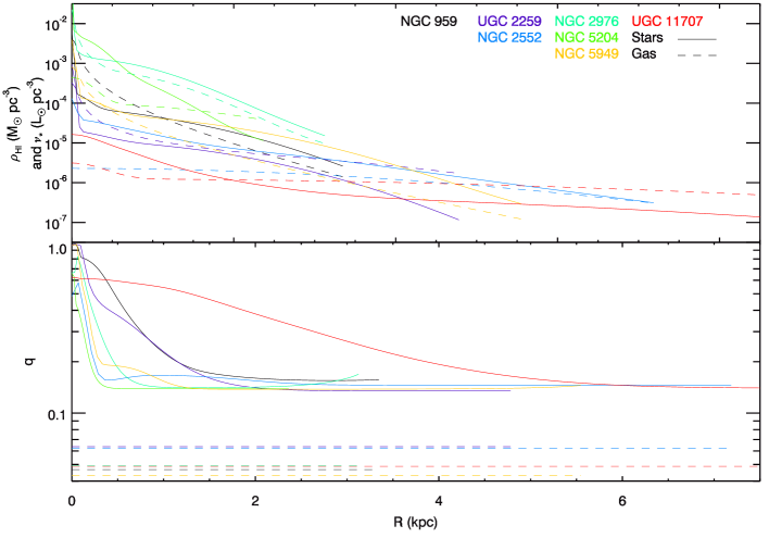
Each galaxy is seen to be rounder at its center, with quite flat, disk-like axis ratios at larger radii. These transitions are robustly seen in the photometry, whether numerically fit or even by eye. In four cases, NGC 2552, NGC 2976, NGC 5204, and NGC 5949, the rounder structure is a compact nuclear star cluster that has negligible influence on the global kinematics of the galaxy. In the remaining three systems, NGC 959, UGC 2259, and UGC 11707 there are larger spheroidal structures that may be either bulges or, more likely, pseudo-bulges. Some of these transitions occur at the same radii where we seek to measure the DM density slopes, so the DM density slope and stellar axial ratio could be covariant at some level. We make a very conservative estimate of the possible bias to the DM rotation curve as follows. We have calculated the rotation curve of the stellar mass from MGE fit terms for both NGC 2976 and NGC 959, and made a second estimate where the axis ratio over the whole radial range is fixed to the flattest value seen at large radii. In the process, we have adjusted the surface density to maintain a constant mass for each MGE component. For NGC 2976, the flatter profile reaches a higher rotational velocity by 1.3 km s^-1 at 150 pc, but converges to the axially-changing case past 200 pc. This difference is easily within the uncertainties on the velocities and therefore has no effect on the DM estimates. In the more extreme case of NGC 959, the flatter distribution produces a rotation curve that is higher by 3–3.5 km s^-1 between 250–1100 pc. While still smaller than our observational errors, this level of bias affects the DM powerlaw slope estimates at the $\Delta\gamma=0.1$ level, comparable to the uncertainties we derive on $\gamma$. We note that a uniformly flat stellar mass distribution is in conflict with our photometry and the best estimates of the axis ratios are given by Figure 1, but small biases resulting from errors in the stellar axis ratios are possible.

2.3. Archival HI Data

Neutral hydrogen can form a significant fraction of the mass at some radii in late-type dwarfs. We gather resolved HI measurements from the literature. In order to account for the mass of helium and metals, we have applied an additional factor to reach $M_{gas}=1.4\times M_{HI}$. We generated MGE terms to represent the HI mass. NGC 959 and NGC 5949 do not have published, resolved HI data. Fortunately, they both have rather low values of $M_{HI}/L_{*,R}$, meaning that the detailed distributions are unlikely to be important to the gravitational potential. We have distributed their total HI masses as exponentials with scale lengths equal to the stellar scale lengths. For these two, the HI mass is effectively absorbed into $\Upsilon_{*}$. For UGC 2259, we have used the radial profile of Figure 5 in Carignan et al. (1988). NGC 2552, NGC 5204, and UGC 11707 have their HI maps presented in Swaters et al. (2003a), and the authors have shared the images. The standard flux-mass equation, with $M_{HI}$ in units of $M_{\odot}$, D as distances in Mpc, and S as the HI flux integral in units of mJy km s^-1, is used as:

$$M_{HI}=236\times D^{2}\times S.$$ (3)

NGC 2976 has been measured in Stil & Israel (2002), and the HI radial profile as presented in Simon et al. (2003) has been used to fit the MGE terms. The MGE fits have been forced to represent thin disks by constraining $q_{j}=0.05$, for the a priori inclination in all cases. The value of $q_{j}$ is comparable to the values of the average vertical scale lengths (Bagetakos et al., 2011) and scale lengths (derived from the table of HI surface densities in Leroy et al. (2008)) for several THINGS dwarf galaxies. From those works, NGC 2976, IC 2574, and NGC 4214 appear marginally thinner (q$\sim$0.03) and NGC 4449 is marginally thicker (q$\sim$0.10). The model mass and axis ratios are shown in Figure 1. We have made no attempt at modeling molecular gas masses. In late-type dwarf galaxies where CO has been observed, the molecular gas is a small component to the total mass (e.g. Simon et al., 2003, 2005).

2.4. Integral Field Spectroscopy

Data were taken with the Visible Integral-field Replicable Unit Spectrograph, Wendelstein model (VIRUS-W) (Fabricius et al., 2008, 2012) mounted on the 2.7m Harlan J. Smith telescope at the McDonald Observatory over several observing runs. VIRUS-W is a fiber-fed, integral-field unit (IFU) spectrograph. We used the high resolution mode which covers 4850Å$<\lambda<$5470Å and delivered $R=8300$ (35 km s^-1) by our measurement of arc lamp lines. We have also made fits to the instrumental resolution by comparing a small number of stars and higher resolution templates and found consistency with the lamp-based measurements. The instrumental resolution measurements are not totally immune to illumination issues as the fibers do not fully scramble signal radially before passing light to the spectrograph. However, the stellar continuum emission in these galaxies is quite regular and even the gas emission is often smoothly varying over several fiber radii. On the 2.7m telescope, the fibers have a diameter of 3$\farcs$1 and the field-of-view, 105″$\times$55″ is one of the largest available for medium resolution IFUs. Observing information is logged in Table 3. In Table 1 we also list the median dispersion observed in the gas emission lines. This measurement is described in §2.5 and its application to estimating a circular velocity is discussed in §3.3. The instrumental dispersion has been measured off arc lamp lines and ranges from 15.4–18.0 km s^-1 for different fibers. The quoted gas dispersions have been corrected to an intrinsic value by subtracting off the fiber-specific instrumental dispersion in quadrature.

Table 3VIRUS-W Data Log

Galaxy	Dates	On-source	$\left<\mu\right>_{e}$	Number of	S/N over
	(UTC)	Exposure	(r-band mag	kinematic	4900-5400Å
		Time (hrs)	arcsec-2)	bins	(pixel-1 bin-1)
NGC0959	23/8/11-27/8/11	10.0	21.9	92	18.9
…	6/2/13-8/2/13
UGC02259	22/12/11-28/12/11	7.0	23.5	43	11.2
…	7/2/13
NGC2552	22/12/11-26/12/11	8.0	23.0	63	16.0
…	5/2/13-8/2/13
NGC2976	16/5/12-20/5/12	6.0	21.4	251	16.7
NGC5204	16/5/12-19/5/12	10.5	21.8	140	18.0
…	5/2/13-8/2/13
NGC5949	20/5/12	3.0	21.4	120	14.7
UGC11707	23/8/11-1/9/11	16.0	23.5	37	17.5

The IFU data were reduced with a pipeline we originally developed for the Hobby-Eberly Telescope Dark Energy eXperiment (HETDEX; Hill et al., 2004, 2008b). The pipeline is named vaccine and is more fully described in Adams et al. (2011). In brief, the pipeline makes the usual CCD reduction steps of bias-subtraction and flat-fielding. Next, it traces the fibers’ centers and measures their cross-dispersion profile. A wavelength solution is fit to arc lamp lines. Finally, a model for the background sky spectrum is made by fitting a bspline (Dierckx, 1993; Kelson, 2003) to all the fibers lacking continuum sources. Careful attention was paid to the quality and robustness of the sky spectrum model driven by the faint emission-line source needs of the HETDEX pilot survey. The bspline fit is particularly well suited to this task as it is stable to outlier datapoints (such as unflagged cosmic rays) and can capture curvature better than a linear interpolation, particularly as we have hundreds of fibers that have sampled the background spectra at slightly offset wavelengths.

2.5. Kinematic Extraction of Stars and Gas

First, the stellar data are binned to achieve sufficient S/N for kinematic extraction. The Voronoi binning scheme of Cappellari & Copin (2003) is used with a target of S/N=12 per pixel per bin. No binning is used for the gas extraction.

We extract kinematics by finding a LOSVD kernel that convolves with a set of stellar template spectra to best match the data. The code we use for this task determines the optimal template weights and makes a maximum penalized likelihood estimate, in pixel space, of the LOSVD (Gebhardt et al., 2000). The LOSVD was initialized as a normally distributed function around the systemic velocity with a standard deviation of 25 km s^-1. A regularization parameter of $\alpha=1$ was used, and experimentation showed that our results were not sensitive to regularizations higher or lower by a factor of three. This code is capable of making non-parametric LOSVD estimates, but for this work we restricted the fits to Gaussian LOSVDs. This is the same method we used in our previous work (Adams et al., 2012), although we have changed the handling of the stellar templates. In some circumstances, nebular gas emission may interfere with this process. One may either fit regions with gas lines or mask them. Since the nebular gas lines (primarily H$\beta$ and [O III]) do not lie in regions with prominent absorption lines and therefore do not coincide with much LOSVD information, we have simply masked 20Å around [O III]4959 and [O III]5007 in the templates. H$\beta$ lies outside our fitting region. We have additionally masked 5195–5205Å in the observed wavelength range due to a variable N I airglow line. The region used in the LOSVD fit was 4900–5350Å. Most of the LOSVD information in this range is coming from three Lick Fe indices (Worthey & Ottaviani, 1997) and the Mg${}_{\textrm{b}}$ triplet. Once the single best fit was found, Monte Carlo simulations through 100 iterations per bin were run to determine the errors on the central velocity and the dispersion.

Template mismatch can bias the kinematic measurements. This is true even for old, single population systems if the templates have the wrong metallicity and especially true for our young, multiple population systems if an improper age or sets of ages are used. If a template is selected that has a different equivalent width (EW) than the data, the fitting process can trade off too-large dispersions with too-strong template lines as a way to distribute the residuals and achieve a statistically better fit. Some checks, and even optional corrections, do exist in the Gebhardt et al. (2000) LOSVD code. One can measure the optimal EW offset and stretch between the data and the best fitting model and choose to fit them as additional parameters. However, it is best to begin with a template set that is as representative of the data as possible. For this reason, we use a small number of composite templates that are fully described in Appendix A. The templates are based on empirical ELODIE spectra (Prugniel & Soubiran, 2001) and stacked to represent a 13.5 Gyr old population and then three populations with a 50% mass fraction from a 13.5 Gyr population and variously a 1 Gyr, 250 Myr, and 50 Myr population.

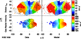
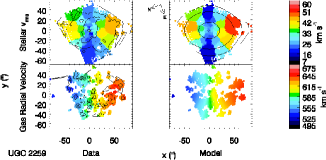
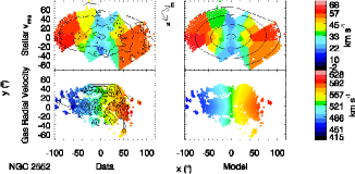
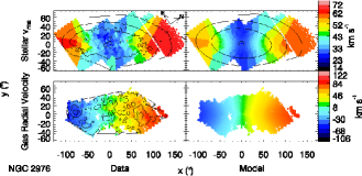
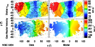
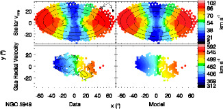
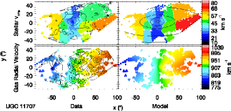
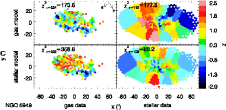
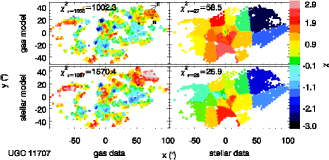
Compared to the stars, the extraction of gas velocities is much simpler. We make a single constrained fit to the H$\beta$, [O III]4959, and [O III]5007 lines. The line widths and radial velocity components are all constrained to hold the same value and are parametrized as Gaussians. The ratio of [O III]5007 and [O III]4959 is fixed to be 2.88 based on atomic physics. We have looked for significantly different velocities between H$\beta$ and the nebular lines and found none. One subtlety is the treatment of underlying Balmer absorption. The effect is minor as the absorption is usually much broader and only slightly offset from the Balmer emission, but we make the proper correction anyhow. We find the stellar kinematic bin to which each fiber belongs. From the stellar template weights and LOSVD values, we form and subtract the best fitting stellar model. Then, we fit the emission lines on the continuum-subtracted data with full error propagation. The velocity maps for the gaseous-traced line-of-sight velocities are shown in Figure 2.

3. Constraints from Dynamical Models

3.1. Model Parameterizations

We have estimated the dynamics model parameters through Bayesian statistical methods. The parameters are quoted in Table 4. In our previous work, we used frequentist parameter estimation with a smaller number of parameters. In the present work, we use Markov Chain Monte Carlo (MCMC) methods to measure parameter constraints and covariances with the python-based software emcee (Foreman-Mackey et al., 2013). Parameters can be estimated either way, but there are several advantages to the Bayesian approach. First, the frequentist approach requires stepping through one or a small number of parameters while optimizing the $\chi^{2}$ metric over the other, nuisance parameters. As is common to general N-dimensional optimization problems, it is difficult to ensure that an absolute, rather than local, minimum has been found. Second, the N-dimensional optimization process is very time consuming. We were able to run optimizations for single parameters and crude grids of parameter covariances, but run-time limits precluded finer grids. Finally, some of the parameters have useful priors, such as the galaxy geometric parameters, and Bayesian analysis can incorporate that additional information.

Table 4Model parameter constraints

	Galaxy	$\log$ M200		c		$\gamma$		$\beta_{z}$		$\Upsilon_{*}$		$i$ (°)		PA(°)		vsys		$\Delta\alpha_{0}$		$\Delta\delta_{0}$		$\sigma_{sys}$
		/M⊙														(km s-1)		(″)		(″)		(km s-1)
Gas-traced	NGC0959	11.06$\pm$	0.23	16.7$\pm$	2.0	0.88$\pm$	0.15	…		1.10$\pm$	0.15	55.2$\pm$	0.1	62.8$\pm$	1.9	597.0$\pm$	0.8	0.8$\pm$	0.4	-0.1$\pm$	0.5	5.6$\pm$	0.7
	UGC02259	11.42$\pm$	0.14	18.2$\pm$	2.6	0.72$\pm$	0.09	…		1.07$\pm$	0.27	41.0$\pm$	0.2	159.9$\pm$	1.5	581.6$\pm$	1.1	-0.8$\pm$	1.0	1.0$\pm$	1.2	5.5$\pm$	0.5
	NGC2552	11.33$\pm$	0.11	18.1$\pm$	2.0	0.38$\pm$	0.11	…		1.01$\pm$	0.19	52.9$\pm$	0.1	57.8$\pm$	0.9	521.9$\pm$	0.7	0.9$\pm$	0.8	1.4$\pm$	0.9	5.7$\pm$	0.3
	NGC2976	11.94$\pm$	0.51	20.6$\pm$	3.3	0.30$\pm$	0.18	…		0.83$\pm$	0.22	62.0$\pm$	0.2	-34.4$\pm$	1.6	5.3$\pm$	1.1	-1.3$\pm$	1.5	-1.5$\pm$	1.3	6.9$\pm$	0.4
	NGC5204	11.36$\pm$	0.16	18.7$\pm$	2.1	0.85$\pm$	0.06	…		1.08$\pm$	0.13	46.8$\pm$	0.1	171.0$\pm$	2.2	201.6$\pm$	0.9	0.2$\pm$	1.0	-0.8$\pm$	1.0	6.6$\pm$	0.7
	NGC5949	11.82$\pm$	0.42	17.5$\pm$	1.9	0.53$\pm$	0.14	…		1.16$\pm$	0.34	62.0$\pm$	0.1	148.5$\pm$	2.0	442.4$\pm$	1.7	1.2$\pm$	0.6	0.2$\pm$	0.7	5.4$\pm$	0.8
	UGC11707	11.49$\pm$	0.18	15.1$\pm$	1.6	0.41$\pm$	0.11	…		1.11$\pm$	0.23	72.7$\pm$	0.1	56.8$\pm$	1.0	899.4$\pm$	1.0	1.4$\pm$	0.7	0.2$\pm$	0.8	7.5$\pm$	0.4
Stellar-traced	NGC0959	11.64$\pm$	0.32	18.5$\pm$	2.4	0.73$\pm$	0.10	-0.05$\pm$	0.20	1.08$\pm$	0.27	55.3$\pm$	0.1	65.4$\pm$	2.2	596.5$\pm$	2.0	-0.6$\pm$	2.0	0.4$\pm$	1.0	3.0$\pm$	1.1
	UGC02259	11.62$\pm$	0.61	16.7$\pm$	5.7	0.77$\pm$	0.21	0.28$\pm$	0.39	1.10$\pm$	0.44	41.1$\pm$	0.2	157.6$\pm$	3.3	578.7$\pm$	2.9	0.9$\pm$	2.3	-0.6$\pm$	3.0	3.3$\pm$	1.2
	NGC2552	11.23$\pm$	0.38	15.8$\pm$	3.6	0.53$\pm$	0.21	0.35$\pm$	0.29	1.24$\pm$	0.55	52.8$\pm$	0.2	56.9$\pm$	3.1	521.9$\pm$	2.7	-1.3$\pm$	2.5	-0.3$\pm$	2.4	3.6$\pm$	0.7
	NGC2976	11.56$\pm$	0.46	17.7$\pm$	2.5	0.53$\pm$	0.14	0.49$\pm$	0.07	0.93$\pm$	0.21	62.0$\pm$	0.1	-33.6$\pm$	3.0	1.5$\pm$	1.3	0.6$\pm$	2.3	0.3$\pm$	1.9	2.3$\pm$	0.6
	NGC5204	11.76$\pm$	0.51	18.3$\pm$	3.3	0.77$\pm$	0.19	0.65$\pm$	0.19	1.30$\pm$	0.42	47.0$\pm$	0.1	172.6$\pm$	3.5	201.4$\pm$	2.2	-0.9$\pm$	2.4	-1.6$\pm$	2.7	2.9$\pm$	1.6
	NGC5949	11.46$\pm$	0.22	17.5$\pm$	1.9	0.72$\pm$	0.11	0.11$\pm$	0.17	1.20$\pm$	0.28	62.1$\pm$	0.1	146.3$\pm$	1.3	441.3$\pm$	1.5	-0.5$\pm$	0.7	-0.1$\pm$	0.7	2.9$\pm$	1.1
	UGC11707	11.13$\pm$	0.37	17.3$\pm$	4.9	0.65$\pm$	0.26	0.34$\pm$	0.26	1.07$\pm$	0.44	72.8$\pm$	0.2	53.1$\pm$	4.0	896.6$\pm$	3.8	1.0$\pm$	4.3	0.5$\pm$	2.9	3.6$\pm$	1.2

Our gas-based models have ten terms: the logarithm of the virial mass, log(M₂₀₀), the concentration c, and the inner density logarithmic slope of a generalized NFW function (gNFW), the stellar mass-to-light ratio $\Upsilon_{*}$, the galaxy inclination, the position angle, the systemic velocity, the offset in right ascension and and declination of the dynamical center from the a prior value, and a systematic uncertainty. Three of these ten parameters describe the DM halo: log(M₂₀₀), c, and $\gamma$. The original NFW density distribution (Navarro et al., 1996b) contains a central cusp with $\gamma=1$. Note that in some of the observational literature, this inner density logarithmic slope is instead named $\alpha$ and the opposite sign is sometimes assigned to the definition. A very general halo profile form was introduced by Hernquist (1990) and explored by Zhao (1996) and Wyithe et al. (2001), where the inner power law, the outer power law, and the sharpness of the transition are all variables. It was shown by Klypin et al. (2001) that these parameters are too degenerate for realistic data to constrain, and a common choice is to leave only the inner power law slope free for a gNFW function. The density of the gNFW function is:

$$\rho(r)=\frac{\delta_{c}\rho_{crit}}{(r/r_{s})^{\gamma}[1+(r/r_{s})]^{3-\gamma}},$$ (4)

where $\delta_{c}$ is the overdensity factor and $\rho_{crit}$ is the critical density of the universe of:

$$\rho_{crit}\equiv\frac{3H^{2}(z)}{8\pi G},$$ (5)

with Hubble parameter $H(z)$ and gravitational constant G. A single integral, which can be reduced to an incomplete gamma function for spherical halos, is given in Dutton et al. (2005) and corrected in Equation 9 of Barnabè et al. (2012), to relate $\delta_{c}$ to c and $\gamma$. We have not fit an Einasto profile (Einasto, 1965; Navarro et al., 2004, 2010) as it does not differ significantly from the gNFW function at our resolution. The stellar-based parameters encompass all the gas-based parameters and further contain a stellar velocity ellipsoid anisotropy term, $\beta_{z}$, defined as

$$\beta_{z}\equiv 1-\frac{\bar{v_{z}^{2}}}{\bar{v_{R}^{2}}}.$$ (6)

We provide fits under an alternative DM functional form commonly used in the literature: the Burkert profile (Burkert, 1995) as

$$\rho(r)=\frac{\rho_{b}}{(1+r/r_{b})(1+(r/r_{b})^{2})}.$$ (7)

This form enforces a DM core. Burkert profiles have been used before, such as to correlate core sizes with other observables in the study of non-CDM models, and therefore its DM parameters will be quoted for comparison to such studies. To make a direct comparison, we have fixed the systematic uncertainties to the values derived for the gNFW fits from Table 4 and run our MCMC pipeline. For most galaxies under study the quality of the Burkert fit, as judged by $\chi^{2}$ with one more degree of freedom relative to the gNFW function and shown in Table 5, is slightly poorer. However, we are unable to rule out the Burkert form from the statistics, and the preference of a galaxy for one profile other another is not always consistent for the two tracers. This is not so surprising since model selection requires a higher statistical threshold ($\Delta\chi^{2}=\sqrt{2\nu}$ for 1-$\sigma$ significance where $\nu$ is the degrees of freedom) than parameter constraint ($\Delta\chi^{2}=1$ for 1-$\sigma$ significance). We give constraints on the two Burkert parameters in Table 6.

Table 5Quality of fit for gNFW and Burkert models

	Gas-traced models				Stellar-traced models
Galaxy	N	gNFW $\chi^{2}$	Burkert $\chi^{2}$		N	gNFW $\chi^{2}$	Burkert $\chi^{2}$
NGC0959	1152	935	1053		92	42.6	47.2
UGC02259	876	752	726		43	27.8	37.9
NGC2552	1848	1765	1836		63	40.2	41.4
NGC2976	1794	1608	1567		251	184.6	180.9
NGC5204	3768	3331	3330		140	80.3	217.9
NGC5949	234	172	177		120	60.3	52.7
UGC11707	1068	1011	1244		37	26.3	17.6

Note. — The number of datapoints are given by N. The degrees of freedom can be obtained with N and the number of fit terms, k. The values are k=9 for the gas-traced gNFW model and 10 for the stellar-traced gNFW model where we have fixed the systematic uncertainty. The Burkert models have k lower by one.

Table 6Burkert DM parameter constraints

	Gas-traced models					Stellar-traced models
Galaxy	$\rho_{b}$		$r_{b}$			$\rho_{b}$		rb
	(M⊙ pc-3)		(kpc)			(M⊙ pc-3)		(kpc)
NGC0959	0.20$\pm$	0.04	1.5$\pm$	0.2		0.22$\pm$	0.05	1.8$\pm$	0.3
UGC02259	0.21$\pm$	0.03	1.7$\pm$	0.1		0.23$\pm$	0.06	1.7$\pm$	0.4
NGC2552	0.10$\pm$	0.02	2.3$\pm$	0.4		0.13$\pm$	0.04	1.6$\pm$	0.3
NGC2976	0.15$\pm$	0.02	2.3$\pm$	0.6		0.15$\pm$	0.02	1.9$\pm$	0.4
NGC5204	0.25$\pm$	0.05	1.7$\pm$	0.3		0.24$\pm$	0.06	1.9$\pm$	0.6
NGC5949	0.18$\pm$	0.04	1.9$\pm$	0.3		0.19$\pm$	0.03	1.9$\pm$	0.2
UGC11707	0.10$\pm$	0.03	2.5$\pm$	0.5		0.17$\pm$	0.05	1.7$\pm$	0.3

Note. — The measured constraints on the central densities, $\rho_{b}$ and the core radii, r_b, in the Burkert function form for DM halos.

The fourth parameter is the stellar mass-to-light ratio in the photometric band specific to the MGE terms, $\Upsilon_{*}$. The two bands we use here are $r$ and $R$. The fifth parameter is the systemic velocity of the galaxy. The next four parameters are geometric: the inclination $i$, the position angle PA, and the offsets from the nominal photometric centers, $\Delta\alpha_{0}$ and $\Delta\delta_{0}$ measured in arcsec. Lastly, the final parameter is a systematic kinematic uncertainty, $\sigma_{sys}$, that is added to the statistical uncertainty for the purpose of calculating model likelihoods. For the gas models this systematic uncertainty applies to the line-of-sight velocity and for the stellar models it applies to the second moment velocities.

The limits on $\Upsilon_{*}$ are formed by considering some stellar populations synthesized with the isochrones of Bressan et al. (2012). We have used a metallicity of [Fe/H]=-0.5, a Chabrier initial mass function (IMF), and considered single burst ages of 100 Myr, 3 Gyr, 13.5 Gyr, and a composite of 10% 100 Myr and 90% 3 Gyr by mass. These four sets, which ought to bound reasonable conditions in dwarf galaxies, correspond to $\Upsilon_{*,R}$=$\left\{0.20,1.60,6.03,0.72\right\}$ and $\Upsilon_{*,r}$=$\left\{0.18,1.26,4.50,0.70\right\}$. Salpeter IMF values will be $\approx$2$\times$ larger. The upper bounds are irrelevant as the best-fit parameters never go so high in the fit. In principle we need a lower bound to protect against an unphysical, massless stellar disk. None of the galaxies are purely young starbursts, and the composite value ought to represent a reasonable lower limit. However, given the uncertainty in the absolute model calibrations of $\Upsilon_{*}$, we will set 0.35 and 10.0 as the limits for both bands. The zeropoint offset between filters is small enough here to ignore. We find that the data themselves require values of $\Upsilon_{*}$ that are sufficiently larger (Table 4) than the lower bound that the bound’s exact value is unimportant.

We assign priors to all the parameters as listed in Table 7. The emcee code operates by distributing “walkers” across the parameter space, moving the walkers around according to the relative likelihoods of the present the proposed parameters without saving the parameters in a “burn-in” phase, and finally recording a number of MCMC samples for each walker under the same type of movement rules. The walkers are initialized to randomized positions as described by the final two columns of Table 7. The systemic velocity and geometric parameters priors are centered around the values listed in Table 1. The priors on the systemic velocities come from an optimally weighted average of our kinematic measurements. The priors on the geometric parameters come from our photometric fits as described in §2.2. We experimented first with placing priors on M₂₀₀ and $c$ via Klypin et al. (2011) and Behroozi et al. (2013), but we found very similar results by adopting the flat priors in Table 7.

The inclinations must have a lower limit enforced to numerically allow deprojection of the MGE terms as discussed in §2.2. Several other parameters have their priors restricted to physically reasonable ranges. All priors are either constant or normal functions.

Table 7Bayesian Priors and MCMC Initialization

	Prior					Initialization
Parameter	Form	Domain	Peak value	Standard deviation		Central value	Standard deviation
M200/M⊙	Uniform	108–1012.5	…	…		1011	1.8$\times$1011
c	Uniform	2.0–40.0	…	…		17.0	3.0
$\gamma$	Uniform	0.0–2.0	…	…		0.6	0.3
$\beta_{z}$	Uniform	-$\infty$–1.0	…	…		0.3	0.3
$\Upsilon_{*}$	Uniform	0.35–10.0	…	…		1.0	0.3
$i$/°	Normal	$i_{min}$–90.0	$i_{0}$ (Table 1)	4.0		$i_{0}$	0.2
PA/°	Normal	0–360.0	PA0 (Table 1)	4.0		PA0	5.0
vsys/km s-1	Normal	-$\infty$–$\infty$	vsys,0 (Table 1)	10.0		vsys,0	5.0
$\Delta\alpha_{0}$/″	Normal	-$\infty$–$\infty$	0.0	3.0		0.0	3.0
$\Delta\delta_{0}$/″	Normal	-$\infty$–$\infty$	0.0	3.0		0.0	3.0
$\sigma_{sys}$/km s-1	Normal	0–$\infty$	5.0	5.0		5.0	5.0
$\rho_{b}$/M⊙ pc-3	Uniform	0–$\infty$	…	…		0.1	0.02
$r_{b}$/kpc	Uniform	0–10	…	…		1.0	0.1

Note. — Column 1 lists the model parameters, column 2 lists the form utilized for the prior probability distributions, column 3 lists the domain over which the priors have non-zero values, columns 4 and 5 list the normal parameters for the relevant cases, and columns 6 and 7 list the normal parameters by which all the parameters are initialized.

Some further details are described in Appendices B–D. There, the details of the MGE computations, some simulations are run to test the recoverability of model parameters, and convergence tests in the length of MCMC chains and the number of parameter space “walkers” are described. The kinematic maps and the best fit gNFW models are shown in Figure 2. The binning can be seen through neighboring fibers having constant velocities in the stellar maps.

Figure 2.— The gas-traced and stellar-traced data and the best fitting gNFW models. Top Stellar kinematic fields in the v_rms parameters. Bottom Gas line-of-sight velocity kinematic maps. Left Data. Right The best fitting models. The contours show logarithmically scaled surface brightnesses for the continuum, on the stellar maps, and the emission lines, on the gas maps. The data-side contours show the actual surface brightnesses and the model-side stellar contour shows the MGE model. Stellar contours are spaced by one magnitude and gas contours by two magnitudes.

3.2. Stellar-based Dynamical Models

We use the Jeans Anisotropic Multi-Gaussian-Expansion (JAM) models of Cappellari (2008) to create the observables that correspond to a particular mass model. The JAM models assume that the velocity ellipsoid can be well represented by a cylindrical coordinate system and that the mass distribution is axisymmetric. Of course, an additional assumption to such models is that the system is virialized. The JAM software solves the Jeans equations. The Jeans equations are formed by taking moments of the collisionless Boltzmann equation. The Jeans equations have a closed form if the shape and orientation of the SVE are fixed. To close the equations, JAM uses the variable $\beta_{z}$ as a free parameter. JAM as provided by M. Cappellari is written in IDL. Our earlier work (Adams et al., 2012) used this version. However, we needed both a faster version and one that could be easily called by the python-based emcee software. Therefore, we rewrote JAM in FORTRAN but without making any substantive changes to the algorithm. At necessary steps within the JAM algorithm, we used the rlft3 routine from Numerical Recipes (Press et al., 1992) for 2D convolution and the dqxgs routine (Favati et al., 1991) in the SLATEC/QUADPACK math library for numerical integration. We ran numerous test cases between the IDL and FORTRAN implementations and always found agreement to better than 1% in velocities for any given mass model. The residuals are likely due to the differences in integration and convolution routines, but they are far below the level of interest for comparison to realistic data. JAM has also been ported into C by Watkins et al. (2013) and is publically available.

3.3. Gas-based Dynamical Models

The tangential velocity of gas may not be a pure probe of the potential’s circular velocity. In a similar fashion to asymmetric drift for stellar tracers, orbiting gas may experience additional pressure. Dalcanton & Stilp (2010) have derived formulae for this situation. The equations are valid if $\sigma_{g}$ is dominated by turbulence, and the gas has an isotropic velocity ellipsoid. Gradients in the surface density of the gas, $\Sigma_{g}$, and the gas dispersion, $\sigma_{g}$, compose a pressure coefficient, $\delta_{P}$, as

$$\delta_{P}=-\left(\frac{d\ln\sigma^{2}_{g}}{d\ln R}+\frac{d\ln\Sigma_{g}}{d\ln R}\right)$$ (8)

$$V^{2}_{c}=V^{2}_{g,\theta}+\delta_{P}\sigma^{2}_{g}.$$ (9)

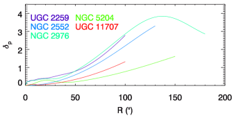
In principle, the finite size of our fibers adds a beam-smearing component to our measured dispersions. However, the largest gradients across a fiber for the observed velocity fields are $\sim$ 5 km s^-1, and the contributed broadening with the round fibers will be less. Since we measure 15$\lessapprox\sigma_{g}\lessapprox$ 20 km s^-1, the beam smearing is insignificant. We find negligible dispersion gradients in all our galaxies; no galaxies show a drop in $\sigma_{g}$ by more than 5 km s^-1 from center-to-edge. The only significant pressure term may be from the radially declining gas density. We must assume that the ionized gas distribution is similar to the neutral gas’s for this computation. Figure 3 shows the pressure support coefficient evaluated for each galaxy. We lack actual resolved HI measurements in NGC 959 and NGC 5949. For the five measured cases, the pressure support coefficient does not reach a value of unity until R$>$50″. At those radii, the rotational velocity is much larger than the gas dispersion so pressure support is not important anywhere. As noted by Dalcanton & Stilp (2010), the effect of this term is to steepen rotation curves, but perhaps not a level that solves the cusp-core problem. Therefore, we conclude that pressure support in the gas is not significant so that we can assume purely circular motion in a thin disk.

Figure 3.— The pressure support coefficient due to neutral gas density gradients. Only if this term took on large values at small radii would the correction to the circular velocity become significant. For the five well-measured cases, the HI is more diffuse than the stellar light, and this term is suppressed at small radii. NGC 959 and NGC 5949 lack resolved HI measurements and are therefore not shown.

We have followed the routines of M. Cappellari, adapted into FORTRAN, to calculate circular velocity for an arbitrary MGE model. Assuming purely circular motion in a thin disk, we can project these circular velocities for each position, given a position angle and inclination, to create a model that can be directly compared to the gas data. The gas-traced models have no use for the stellar velocity anisotropy, but all the other input parameters are shared with the stellar-traced models.

The models previously presented have assumed axisymmetry. Dropping this assumption adds significant complexity. In order to model triaxial structures through stellar kinematics, the best option is to use triaxial Schwarzschild codes, for which van den Bosch et al. (2008) is the current standard. The code has primarily been used to assess the robustness of supermassive black hole mass estimates in the presence of triaxial halos. The main limitation is that only static potentials can currently be modeled. The code could profitably be employed to more generally fit triaxial halo shapes in our sample, but it cannot fit structures with a pattern speed such as bars. We hypothesize that bars may be a significant dynamical perturber to the gas kinematics, but less so to the hotter stellar kinematics. We do not attempt to model triaxial structure through stellar kinematics herein.

Fortunately, the problem of triaxial structure affecting gaseous kinematics has been extensively studied. The general solution for an arbitrary number of harmonic terms is presented in Schoenmakers et al. (1997). A general solution named DiskFit, accompanied by software, has been given in a set of papers (Spekkens & Sellwood, 2007; Sellwood & Sánchez, 2010). The basic idea is that a bisymmetric potential component, $m=2$, will contribute to the sky-projected harmonic modes of $m^{\prime}=m\pm 1$. This leads to Equation 5 in Spekkens & Sellwood (2007)

$$v_{rad}=v_{sys}+\sin i(v_{1,t}\cos\theta- v_{2,t}\cos(2(\theta-\phi_{b}))\cos\theta$$

$$- v_{2,r}\sin(2(\theta-\phi_{b}))\sin\theta),$$ (10)

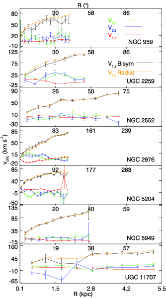
where $\theta$ is relative to the major axis and $\phi_{b}$ is the angle between the projected major axis and the long axis of the triaxial structure, assumed to be a bar by Spekkens & Sellwood (2007). When data sets show more complex structure than simple tangential motion, two simple choices present themselves. One may fit the motion as radial, first-order motion (inflow or outflow) or as the tangential and radial terms of a bisymmetric distortion. Spekkens & Sellwood (2007) used data on NGC 2976 to explain the kinematic twist with each model and showed that the derived circular velocity curve is sensitive to this choice. However, the gas kinematics can be fit nearly as well with either choice, and the interpretation is degenerate. Our stellar kinematic data on NGC 2976 show a powerful route toward breaking this degeneracy and favor the bisymmetric distortion fit to the gas. A primary goal of this study is to determine whether such bisymmetric distortions are consistently biasing the inferred potentials in late-type dwarf galaxies or if NGC 2976 is an outlier.

We have adapted a tilted ring code to perform the same operations as DiskFit. We fit both radial and bisymmetric models to each of our galaxies. The position angles, inclinations, and centers were left free in the fits. Errors were estimated with 100 bootstrap resamplings. The fits are shown in Figure 4. We recover the result from Spekkens & Sellwood (2007) that NGC 2976 has a substantially different rotation curve under the two parametrizations, with the bisymmetric rotation curve having larger rotational velocities at smaller radii. UGC 11707 shows unrealistic behavior, but the problem is only present in the second smallest radial bin for both models. The gas velocity map of UGC 11707 shows a small pocket of high velocity gas at 12″ off the major axis. The gas emission in this bin is quite patchy. The high velocity measurement is real and significant, but it is unlikely to truly be a signal of regular, global, gravitationally dominated motion. The remaining five galaxies show strong agreement in the radial and bisymmetric models. Some bar and viewing angles can still hide kinematic features, but we see good evidence in one of seven galaxies for bars that produce a significant bias in the rotation curves.

Figure 4.— DiskFit models for all seven galaxies. Both an $m=1$ model with a radial component, v_1,r, and a bisymmetric, $m=2$ model with radial, v_2,r, and tangential, v_2,t, components are fit. The bisymmetric model can represent a bar. Given the much larger uncertainties in the first order tangential velocity for the bisymmetric model, the two circular velocity curves are generally consistent. NGC 2976 The two fits are similar to those in Spekkens & Sellwood (2007). The bisymmetric model returns larger velocities at smaller radii as a cuspier model would produce. The statistical quality of the two fits are indistinguishable, but the stellar-traced mass models are more compatible with the bisymmetric gas models. UGC 11707 Both models fit a large tangential velocity to the bin at R=1.1 kpc. However, the fit is unlikely to represent global, gravitational-driven motion. Due to dust and patchiness in the gas distribution, the azimuthal coverage for this ring is poor and the velocities are distinct from the overall kinematics of the galaxy. A small pocket of high velocity gas is likely driving this unrealistic solution. Within the large uncertainties, the two fits are consistent.

3.4. MOND parameter estimation

Modified Newtonian Dynamics (MOND) was first proposed as an alternative explanation to dark matter for the flat rotation curves of galaxies at large radii by Milgrom (1983). The one additional physical constant required by MOND is $a_{0}$, the small acceleration at which objects start to deviate from Newton’s Laws. The modification is usually written as $\mu(a/a_{0})\times a=GMr^{-2}$ with a common choice of $\mu(a/a_{0})=(1+a_{0}/a)^{-1}$. Under this form, the acceleration at the radius where a dark matter fit has an enclosed DM mass fraction of one-half can be interpreted instead as the value for $a_{0}$. We have made such an estimate from our data for the gNFW fits. We find $a_{0}=$0.78$\pm$0.37$\times$10^-10 m s^-2 from the gas-based data and $a_{0}=$0.56$\pm$0.40$\times$10^-10 m s^-2 from the stellar-based data. For both, we find root-mean-squares of 0.57$\times$10^-10 m s^-2, meaning that our data appear to favor a non-constant value of a₀. The significance for a non-constant value, however, is modest as 5/7 and 3/7 of the gas-based and stellar-based measurements deviate from the central estimate by 1-$\sigma$ significance.

4. Interpreting the Mass Models

4.1. Agreement Between Kinematic Tracers

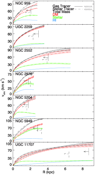
We find that the posterior mass models inferred from the gas and stars are not always consistent. However, the density profiles are usually consistent. We show the inferred rotation curves for both kinematic tracers in Figure 5. The curves, their decomposition into various mass components, and the 1-$\sigma$ ranges around the total rotation curves are created by averaging rotation curves from 1000 of the MCMC samples. NGC 2552 shows clear disagreement with the gas-traced asymptotic velocity being larger than the stellar-traced one, while the situation is reversed for NGC 959. We have tried evaluating the stellar-traced models against the gas data and vice versa, and the fits for these two galaxies are truly poor representations of the swapped data sets. In our current framework, we have no set of parameters that can bring the potentials into agreement. We speculate that the two potentials could be brought into better agreement by adding non-spherical structure to the DM halo, as the gas and stars will react differently. The simplest approach would be to make oblate or prolate DM halos in JAM. A constant ellipticity to the DM halo would shift the normalization of the rotation curves (Simon et al., 2005). More complicated structure, such as ellipticity varying as a function of vertical height, could change the rotation curve shape, although a significant shape change could only come about by very contrived alignments, vertical scalings, and strong ellipticity gradients. Since the gas is the thinnest component, a constant ellipticity shift to the DM will change the gas-traced normalization more strongly than the stellar-traced one. This general problem is beyond the scope of this work. NGC 2976 shows modest, but significant, disagreement in the same sense of the radial and bisymmetric DiskFit models and as we found in Adams et al. (2012). The stellar-traced rotation curve has larger amplitude at smaller radii. The other four galaxies, UGC 2259, NGC 5204, NGC 5949, and UGC 11707 show fairly good agreement.

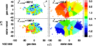
The data regions driving each fit can be seen in Figure 6. There, the residuals to the gas and stellar kinematic maps are shown along with the residuals from the parameter set selected by the alternate tracer.

Figure 5.— The rotation curves for the best fit parameters from the gas-traced and stellar-traced data. The median rotation curves for the various parts of the mass budget are shown as well as the 1-$\sigma$ confidence bands. Arrows are drawn to show the largest radius bin for each tracer. The circular velocity curves have been fit for each tracer as described in the text. For the gas data, the fit is made to the observed rotational velocity field. For the stellar data, the fit is made to the quadrature sum of rotational velocity and dispersion. NGC 959 The two tracers do not agree in their large-radii normalizations. The disagreement is robustly contained in the data, and is likely due to our models not containing necessary complexity, such as from non-spherical DM halos. UGC 2259 The gas-traced model appears cuspier. NGC 2552 The large-radii normalization again disagrees between the two models. NGC 2976 A subtle but significant disagreement exists in the shape of the rotation curves. The disagreement is mainly in normalization with $\Upsilon_{*}$ fit differently between the two models. If a fixed value is used, the disagreement is primarily in a cuspier shape to the stellar-traced model. NGC 5204 The two tracers show excellent agreement in their mass models. NGC 5949 The two tracers show reasonable agreement in their mass models, but with the stellar-based model being modestly more cuspy. UGC 11707 The two tracers again show modest disagreement at small radii, but the large error bars may explain the difference.

Figure 6.— Quality-of-fit $\chi$ maps. Left The line-of-sight gas velocities compared to models. Right The stellar second moment velocities compared to models. Top Model made with the best-fitting parameters based on the gas data. Bottom Model made with the best-fitting parameters based on the stellar data. The total $\chi^{2}$ values and degrees of freedom are written in every panel. These plots indicate how strongly the two tracers disagree and show the regions that are causing the disagreement, when present. The major conflict in NGC 959 is that the stellar model robustly has a larger asymptotic velocity than the gas. The two models for UGC 2259 are quite similar and without structured residuals in the swapped models. For NGC 2552, the two models are quite similar, with most of the structured residuals in the swapped models attributable to slightly different kinematic centers and PAs. The two models for NGC 2976 show modest disagreement, with most of the structured residuals in the swapped models attributable to slightly different kinematic centers and $\gamma$. The two models for NGC 5204 are quite similar. For NGC 5949, the two models show modest disagreement, with most of the structured residuals in the swapped models attributable to differences in $\gamma$. Finally, the two models for UGC 11707 show modest disagreement. The main cause is a difference in $\gamma$, but even it is compatible within the errors between the two tracers.

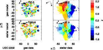
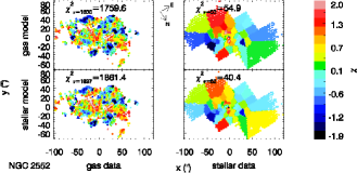
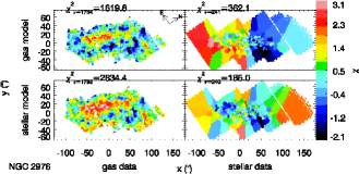
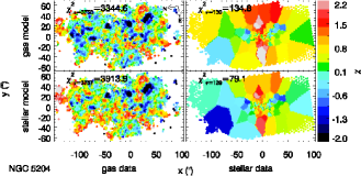
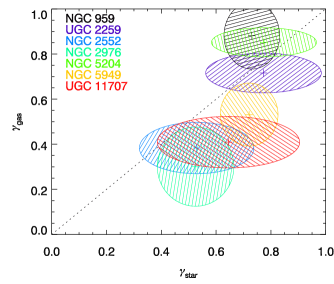
The logarithmic DM slopes derived from the gas and stellar tracers are compared in Figure 7. The data agree fairly well with the simple one-to-one relation. The most cored halos show a small bias toward being steeper from the stellar-traced models, but there is no doubt that several galaxies are incompatible with NFW profiles. NGC 2976 agrees with the one-to-to relation within the uncertainties, in contrast to our previous work. The gas-traced model has become steeper, because the model has swept over several PAs and not modeled non-circular terms, and the stellar-traced model has become shallower because the stellar photometry and mass has increased as discussed in §4.2. Two galaxies are outliers beyond 1-$\sigma$ significance, which is expected from normal statistics alone. NGC 5949 looks more cuspy from the stellar-traced models. NGC 5949, however, does not have evidence for a bar from the gas kinematics field and the discrepancy is harder to explain. It may be that more complex triaxial structure is causing this subtle (barely 1-$\sigma$) difference between the two tracers, or the model disagreement may be due to random chance.

Figure 7.— The logarithmic DM slopes, $\gamma$, as derived from the gas- and stellar-traced models. The 2D error ellipses represent 1-$\sigma$ uncertainties. The constraints on $\gamma$ are generally consistent between the two data sets. The line shown is the one-to-one relation expected if both tracers are unbiased.

4.2. Comparison with Literature Density Profile Measurements

In Adams et al. (2012) (hereafter A12) we presented lower quality data on NGC 2976. In addition to acquiring higher resolution, higher S/N data, we have also improved the analysis methods by adopting a Bayesian approach. We first address the question of whether the A12 data and analysis are consistent with our new results on NGC 2976, and then broaden this comparison to consider the other galaxies with published density profile slopes in the literature.

We find that the qualitative result with the stars in NGC 2976 reporting a steeper DM halo than the gas remains in the A12 data, but the quantitative limits on the logarithmic slope of the density profile change. The most substantial change is that the SDSS photometry on NGC 2976 report double the luminosity as the SINGS image originally used. The SDSS photometry is in better agreement with that from Simon et al. (2003). From Figure 13 of A12, it can be seen that because of the degeneracy between the stellar mass-to-light ratio and the density profile slope, such a shift in the stellar mass decreases the most likely value of the logarithmic slope to $\sim$0.5. We ran the new MCMC pipeline with the A12 data and MGE components and recovered the same best-fit value as in Figure 13 of A12. Next, we ran the A12 data with the new pipeline but with the updated stellar luminosity. The central estimates for $\gamma$ with the A12 data and A12 analysis, the A12 data and new analysis, and new data and new analysis, respectively, are: 0.9, 0.62, and 0.53. The facts that the A12 data barely resolved the dispersions, were binned differently, and lacked the thorough parameter search from the MCMC pipeline do not make a significant difference given the strong consistency between the A12 and new constraints when using a common MGE model. In the case of a zero mass, or very low mass, disk for NGC 2976, the disagreement between the stellar and gaseous kinematics remains significant. The better agreement in $\gamma$ between the two tracers for NGC 2976 achieved in the present analysis (Figure 7) is due to the two models settling on different values of $\Upsilon_{*}$ (Table 4).

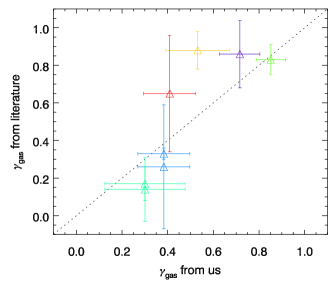
Five of the remaining six galaxies have measurements of $\gamma$ available in the literature. We have plotted the literature values and our measurements in Figure 8.

For the sixth galaxy, NGC 959, no numerical value of $\gamma$ has been published. NGC 959 was fit with pseudo-isothermal (cored) and NFW profiles in Kuzio de Naray et al. (2008) under a zero disk mass assumption. There was a very modest statistical preference for the cored fit, with $\chi^{2}_{r}$ values of 1.2 and 1.7, respectively.

UGC 2259 was measured by de Blok et al. (1996) and only fit with a pseudo-isothermal function. They found a core size of 0.4–1.2 kpc depending on the value of $\Upsilon_{*}$. Swaters et al. (2003a) measured UGC 2259 to have $\chi^{2}_{r}$ values of 1.8 and 2.3 for pseudo-isothermal and NFW functions respectively. They also fit a gNFW function with $\gamma=0.86\pm 0.18$. For UGC 2259, we measure $\gamma=0.72\pm 0.09$ from the gas and $\gamma=0.77\pm 0.21$ from the stellar kinematics, in excellent agreement with Swaters et al. (2003a).

NGC 2552 was fit by de Blok et al. (2001a) to have $\gamma=0.33\pm 0.03$. Swaters et al. (2003a) measured NGC 2552 to have $\chi^{2}_{r}$ values of 1.5 and 3.4 for pseudo-isothermal and NFW functions. They also fit a gNFW function with $\gamma=0.26\pm 0.33$. Kuzio de Naray et al. (2006) find moderately poor pseudo-isothermal fits ($\chi^{2}_{r}=3.8$) but very poor NFW fits ($\chi^{2}_{r}=40$). Kuzio de Naray et al. (2008) reinforce these findings for additional values of $\Upsilon_{*}$. Spano et al. (2008) find that the pseudo-isothermal ($\chi^{2}_{r}=2.5$) and NFW ($\chi^{2}_{r}=2.9$) functions fit the data to a similar level. We find slightly steeper profiles using both the gas ($\gamma=0.38\pm 0.11$) and the stars ($\gamma=0.53\pm 0.21$), but the results are consistent within the uncertainties.

NGC 2976 was fit in Simon et al. (2003) to have $\gamma=0.17\pm 0.09$ for a minimal disk or $\gamma=0.01\pm 0.13$ for a maximal disk. de Blok et al. (2008) made fits with $\Upsilon_{*}$ freely determined and found $\chi^{2}_{r}=0.5$ for a pseudo-isothermal fit and $\chi^{2}_{r}=1.7$ for a NFW fit. Both fits had their parameters run into physical boundaries, with the pseudo-isothermal core radius going to infinity and the NFW concentration going to zero. As discussed above, we find a value in NGC 2976 steeper than that presented in Simon et al. (2003), especially for our stellar-traced value. Our present value is shallower than that presented in Adams et al. (2012).

NGC 5204 was measured by Swaters et al. (2003a) to have $\chi^{2}_{r}$ values of 1.0 and 1.7 for pseudo-isothermal and NFW functions. They also fit a gNFW function with $\gamma=0.83\pm 0.16$. Spano et al. (2008) find that the pseudo-isothermal ($\chi^{2}_{r}=0.6$) model fits moderately better than the NFW ($\chi^{2}_{r}=2.1$) function. Our gas-traced measurement ($\gamma=0.85\pm 0.06$) is spot-on with the Swaters et al. (2003a) value and our stellar-traced value ($\gamma=0.77\pm 0.19$) also agrees within the uncertainties.

Simon et al. (2005) make a disk-subtracted fit to NGC 5949 and find $\gamma=0.88$. NGC 5949 is fit by Spano et al. (2008) to a similarly likely level with pseudo-isothermal ($\chi^{2}_{r}=1.0$) and NFW ($\chi^{2}_{r}=1.4$) functions. Our measurements for NGC 5949 ($\gamma=0.53\pm 0.14$ from the gas and $\gamma=0.72\pm 0.11$ from the stars) are shallower than the value determined by Simon et al. (2005), although not by a large margin when the combined uncertainties are taken into account.

Swaters et al. (2003a) measured UGC 11707 to have $\chi^{2}_{r}$ values of 1.5 and 0.5 for pseudo-isothermal and NFW functions. They also fit a gNFW function with $\gamma=0.65\pm 0.31$. Spano et al. (2008) finds a moderately better pseudo-isothermal ($\chi^{2}_{r}=2.6$) than NFW ($\chi^{2}_{r}=3.8$) function fit for UGC 11707. We measure $\gamma=0.41\pm 0.11$ for the gas kinematics and $\gamma=0.65\pm 0.26$ for the stellar kinematics of UGC 11707, in agreement with the value from Swaters et al. (2003a) given the large uncertainty.

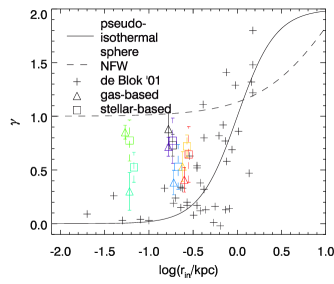
Finally, we consider logarithmic density slopes compared to the spatial resolution of the data. It has been shown before (de Blok et al., 2001a) that data taken with insufficient spatial resolution can bias the measurement of fully cored systems to higher values of $\gamma$. Figure 1 of de Blok et al. (2001a) looked at this issue through data compiled from three earlier studies. In Figure 9, we add our data to this plot. One can see that our data lie far below the turnoff where biases occur for reasonable core sizes. Our results are therefore not dependent on spatial resolution. Additionally, our data occupy a space not populated by the de Blok et al. (2001a) study. We genuinely find systems intermediate between cores and cusps rather than fully cored halos.

Figure 8.— The logarithmic DM slopes, $\gamma$, as fit from gas kinematics in this work and from all available literature values. The only measurement significantly discordant from a one-to-one relation is the NGC 5949 measurement from Simon et al. (2005) being cuspier. Our stellar-based measurement is closer to the Simon et al. (2005) value.

Figure 9.— Demonstration that the spatial resolution of the data is sufficient to discriminate between models. The crosses are from the compilation of data in Figure 1 of de Blok et al. (2001a). When the spatial resolution is poor, as indicated by the innermost radial data point, a cupsy measurement can be obtained even if the true density profile contains a core, like the pseudo-isothermal sphere. Our data are shown with the color coding per galaxy as in Figure 7. The innermost radius is determined by adding the seeing to the fiber radius in quadrature. All of our data have high enough spatial resolution that fully cored profiles would have been detected if present. The solid curve assumes a core radius of 1 kpc for the pseudo-isothermal sphere, and the dashed curve assumes c=10 and V₂₀₀=100 km s^-1 for the NFW functional form.

5. Discussion

5.1. The Distribution of Logarithmic Density Profile Slopes

Because theoretical models generally do not attempt to reproduce the detailed properties of individual galaxies, the best way to compare observational results with theoretical predictions is to consider the distribution of dark matter density profile slopes. The previously published values are $\gamma=0.73\pm 0.44$ from five galaxies analyzed by Simon et al. (2005) and $\gamma=0.29\pm 0.07$ determined for seven THINGS dwarf galaxies by Oh et al. (2011b). Our sample of seven galaxies yields $\gamma=0.67\pm 0.10$ for the stellar kinematics and $\gamma=0.58\pm 0.24$ for the gas. Interestingly, our mean slope using either tracer is significantly steeper than the THINGS H I measurements, but we find a narrower distribution than Simon et al. (2005). In fact, the uncertainty on the mean value of $\gamma$ we derive includes both intrinsic and measurement contributions, so that the intrinsic scatter from galaxy to galaxy appears to approach zero. These data are thus consistent with a universal profile, but not with the slope predicted by dark matter-only N-body simulations in $\Lambda$CDM. Of course, our sample is still small enough that we could have failed to include intrinsically cored or cuspy galaxies simply by chance.

To obtain the best available estimate of the distribution of density profile slopes, we combine our sample with the highest-quality literature measurements, including only objects for which high-resolution two-dimensional velocity fields are available. We do not include results from Kuzio de Naray et al. (2008, 2009) because they do not derive logarithmic density slopes. Simon et al. (2005) observed three galaxies that do not overlap with our sample: NGC 4605 ($\gamma=0.78$), NGC 5963 ($\gamma=1.20$), and NGC 6689 ($\gamma=0.79$). The other comparable data set is that of Oh et al. (2011b). We note several important differences between our methodology and theirs. First, the THINGS dwarfs have lower stellar masses than our targets, but both are in the range over which SN feedback models are predicted to be effective at changing the DM profiles. Second, rather than fitting a density profile to the full rotation curve or velocity field, Oh et al. (2011b) measure the density profile slope by fitting a power law only to the innermost $\sim 5$ points of the rotation curve ($r\lesssim 1$ kpc), which are the ones potentially most subject to systematic uncertainties and assumptions about the baryonic mass distribution. Most of the THINGS sample also exhibits serious kinematic peculiarities that may bias the inferred density profiles. For example, five of the seven galaxies (NGC 2366, Holmberg I, Holmberg II, DDO 53, DDO 154) have significant kinematic asymmetries between the approaching and receding sides of the galaxy, two have substantial non-circular motions (IC 2574, NGC 2366) , and one has a declining rotation curve (M81dwB). If we include only the best behaved THINGS galaxies, Ho II and DDO 154, with the Simon et al. (2005) sample and our new results, that leaves us with a total sample of 12 objects. This combined set produces a mean slope of $\gamma=0.63$ and a scatter of $\sim 0.28$, essentially independent of whether we use gaseous or stellar kinematics. We suggest that these values represent the best current constraints on the observational distribution of dark matter density profiles on galaxy scales. These values are strikingly similar to those measured for the dark matter profiles of galaxy clusters by Newman et al. (2013a).

5.2. Systematic Uncertainties

Our data have reduced sensitivity to some sources of systematic error and are equally sensitive to other systematic errors as previous data sets. By using stellar kinematics, we are potentially adding an additional systematic through the vertical orbital anisotropy. The tests presented in Appendix D were designed to test for this problem through simulations, and the level of systematic bias in $\gamma$ is found to be $<0.1$. The properties of high spatial resolution and two dimensional kinematics in our data retire a swath of systematic risks relating to locating the kinematic center and major axis alignment. While binning in our stellar kinematic extraction could plausibly be a risk, we find again from the simulations that this introduces no bias. Gas-based analysis is usually performed under the assumption of infinitely thin, planar, and circular motion. Our stellar-based analysis is predicated on the less restrictive assumptions of a steady-state, axisymmetric potential. While we find cases that can be resolved by breaking the usual gas modeling assumptions, the biases in $\gamma$ are small and comparable to the statistical uncertainties. Three sources of systematic error to which we, and other methods, are still potentially susceptible are triaxial DM halo structure (Valenzuela et al., 2007; Kowalczyk et al., 2013; Valenzuela et al., 2014), M/L_∗ variations with radius, and more complex orbital anisotropy than can be fit with a single $\beta_{z}$ term. A fourth, minor concern is that the assumption in the JAM models of a cylindrically aligned dispersion ellipsoid is invalid. This is unlikely to be important because regions near the disk plane will be cylindrically aligned and the extra-planar regions will only become influential at very high inclinations. We note that the main effect of a constant ellipticity triaxial halo is to change the rotation curve normalization (Simon et al., 2005) and the indications from color and Lick index gradients are that M/L_∗ gradients are small or absent in our galaxies. We do not identify any source of systematic error that can plausibly affect our measurements of $\gamma$ at a significant level.

5.3. Inner DM Surface Density

Many authors have found that the inner DM surface density ($\rho_{b}\times r_{b}$) takes on a constant value for all galaxies and galaxy clusters measured. Donato et al. (2009) determine this constant to be 141${}^{+82}_{-52}$ M_⊙ pc^-2. We find an average of $\rho_{b}\times r_{b}=$321 M_⊙ pc^-2 from the gas and $\rho_{b}\times r_{b}=$341 M_⊙ pc^-2 from the stars. One galaxy, NGC 2552, lies removed from these averages by 1.5$\sigma$ in both tracers, and no others lie beyond 1$\sigma$. Within the limits of our errors and small sample, the inner DM surface density is constant but significantly different than previous estimates. Additionally, the inner DM surface densities of M31 dSphs appear offset from those of the MW (Walker et al., 2010) and the DM surface density may not be a constant.

5.4. Correlations with DM Halo Profile

Although one might expect correlations with baryon content or stellar populations, we know of no secondary observables that are predicted to correlate with the logarithmic DM slope in the SN feedback or non-CDM models. Lacking firm theoretical guidance, we explore several parameters for clues to the underlying physics. We show the stellar-traced logarithmic DM slopes compared to the orbital anisotropies in Figure 10. NGC 2976 and NGC 5204 have significantly flattened stellar velocity ellipsoids as seen by previous studies (Appendix C), but two others are intermediate and the remaining three galaxies are significantly more isotropic. There is an anti-correlation between $\gamma_{star}$ and $\beta_{z}$, however the large error bars leave only a modest significance to the correlation. We next plot the logarithmic DM slope against the relative mass in HI and stars in Figure 11. The SN feedback models make repeated starbursts at high redshifts. We cannot assess whether galaxies having experienced such disruptive events should still be expected to be gas-poor or whether subsequent accretion would wash out the signal. However, a strong trend between cored-ness and gas-deficit would perhaps be an indicator for the SN mechanism. The strength of correlation between $\gamma$ and the gas content is quite weak, and we can only exclude a very strong positive correlation. We have also calculated the HI gas mass internal to 2 $R_{d}$ relative to the total mass as a way to investigate the central HI content that may be more sensitive to SN feedback. The results look like a scaled version of the total HI fraction.

Figure 10.— The stellar-based logarithmic DM slopes and vertical orbital anisotropies. A maximum likelihood linear fit to the stellar-based values is largely unconstrained, but shown by the line and shaded 1-$\sigma$ confidence interval. The color coding per galaxy is the same as in Figure 7.

Figure 11.— Investigation of correlations with the logarithmic DM slope, $\gamma$. The color coding per galaxy is the same as in Figure 7. The maximum likelihood linear fit to the stellar-based values is shown. Stellar-based values are dotted and gas-based values use solid lines. Top The ratio of HI to stellar mass. The data do not make a strong constraint and only exclude the strongest of correlations. The best fit is anti-correlated. SN feedback models would presumably predict a positive correlation between these values, if anything. More data to strengthen the anti-correlation and robust model predictions are necessary to investigate this preliminary evidence. Bottom The DM mass fraction within a sphere of twice the stellar scale radius. The data exclude an anti-correlation.

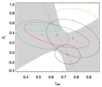
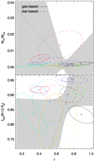
We calculate the DM, stellar, and HI masses within two scale scale lengths. One non-analytic integral (Equation 5 of Wyithe et al., 2001) was required to compute the gNFW enclosed mass. The DM fraction is compared to the logarithmic DM slopes in Figure 11. There is a weak correlation, but one also consistent with the uncertainties and a null hypothesis. This correlation may also naturally arise without a feedback mechanism because more-cored DM halos have lower central masses. We also look at the Burkert core sizes compared to the stellar disk scales in Figure 12. The self-interacting DM models of Kaplinghat et al. (2013) predict correlations between disk scale length and DM core size at high baryon fraction but anti-correlation between DM core size and disk mass. For our sample drawn from a range of disk masses and intermediate baryon fractions, the second trend is most important and would imply an anti-correlation in DM core size and stellar disk scale. However, we find neither a positive nor negative correlation in our data.

Finally, we investigate other parameters that have a long history of being correlated in N-body and semi-analytic models. In Ferrero et al. (2012), the halo masses of dwarf galaxies are measured and have smaller DM halos over the range $10^{6}<M_{*}/M_{\odot}<10^{7}$ than the semi-analytic models of Guo et al. (2011) predict. The two likely explanations for their data are that vast numbers of dwarf galaxies are being missed by current surveys or that feedback is able to dramatically reduce the DM halo masses in dwarfs. However, at the stellar mass values studied in our work, the Ferrero et al. (2012) measurements indicate agreement with semi-analytic modeling. We show the total stellar mass compared to the DM mass for our sample in Figure 13. The stellar mass to halo mass is a strong prediction of the data-tuned models of Behroozi et al. (2013). We find that on average, our measurements agree with the $z=0$ models. Another robust prediction from N-body models is the DM mass-concentration relation. Since our data do not adhere to the NFW functional form, it is not meaningful to compare our values of $c$ with those from simulations. Alam et al. (2002) have presented a non-parametric overdensity parameter, $\Delta_{V/2}$, to address exactly this issue. The value simply represents the overdensity relative to the critical density at the radius where the circular velocity equals one-half the halo’s maximum. This value can be derived numerically for an arbitrary density profile. We measure the value for our gNFW fits in Figure 13 as compared to N-body model predictions. Note that we have assigned V${}_{\textrm{max}}$ to the circular velocity at our largest measured radius for this plot. If we instead calculate V${}_{\textrm{max}}$ from the full gNFW function, $\Delta_{V/2}$ becomes lower but several galaxies take on V${}_{\textrm{max}}$ values significantly larger than their H I linewidths would indicate. The two likely causes of this mismatch are that neither our data nor the H I linewidths are reaching the maximum velocity in the halo or the virial mass cannot be robustly constrained by data from the central few kpc and the gNFW fits are mitigating the residuals at small radii by biasing high M₂₀₀ which is acceptable statistically as the large radii bins have large uncertainties. The mismatch we see between V${}_{\textrm{max}}$ and V${}_{\textrm{flat}}$ is not the same as the core-cusp issue because our galaxies are not underdense in $\Delta_{V/2}$ by either measure. The N-body predictions come from NFW fits and the M₂₀₀-c relation for central halos from the Bolshoi simulations Klypin et al. (2011). Surprisingly, our measurements lie at or above the predictions. $\Delta_{V/2}$ has been seen to lie below $\Lambda$CDM predictions in Alam et al. (2002) and again in Simon et al. (2005), albeit within 1-$\sigma$ of the cosmic scatter. Contrary to many previous results, the galaxies in our sample do not seem to be underconcentrated relative to theoretical predictions. While the logarithmic DM slopes indicate a core/cusp problem, $\Delta_{V/2}$ is sensitive to larger radii regions and does not indicate a deficiency in DM mass. The mismatch we see between V${}_{\textrm{max}}$ and V${}_{\textrm{flat}}$ is not the same as the core-cusp issue because our galaxies are not underdense in $\Delta_{V/2}$ by either measure. Together, $\gamma$ and $\Delta_{V/2}$ limit the radial range of mass redistribution and energy input permitted by any feedback model.

We have quantified possible correlations based on the stellar-traced kinematic models in Table 8. The parametrization is limited to a linear model. Since we have errors in both dimensions and often correlated errors, we have used a general maximum likelihood solution for the fit parameters instead of the normal equations for linear least squares. We evaluate the likelihood for each model by finding the orthogonal residual to the line of each datapoint and the projection of the error ellipse along the same direction, which when divided, form the deviates. The sum of the squares of the deviates are then minimized and the covariance matrix is found through a non-linear least-squares solver. As suggested in Hogg et al. (2010), we have fit the terms $\theta$ and $b_{\perp}$ instead of a traditional slope and intercept. Doing so treats all slopes as equally likely a priori with implicit, flat priors on $\theta$ and $b_{\perp}$. The simple relation,

$$y=x\times\tan\theta+\frac{b_{\perp}}{\cos\theta}.$$ (11)

gives the linear fit for variables $x$ and $y$ in terms of $\theta$ and $b_{\perp}$. The dependent and independent variables and $b_{\perp}$ share the same units for each fit except for the [MgFe’] fit where $b_{\perp}$ has units of Å. $\theta$ is given in radians. We have propagated the uncertainties through Taylor expansion to the dependent variable for all figures with a useful constraint. When no confidence interval is shown, the intervals fill nearly the entire plot range and are mentioned in the caption.

Table 8Measured parameter correlations.

Dependent	Independent	$\theta$	$b_{\perp}$	$\sigma^{2}_{\theta}$	$\sigma_{\theta b_{\perp}}$	$\sigma^{2}_{b_{\perp}}$	Figure
parameter	parameter						number
$\beta_{z}$	$\gamma$	1.76	-0.71	0.057	-0.0044	0.0033	10
$M_{HI}/M_{tot}$	$\gamma$	3.08	-0.044	0.014	0.0098	0.0068	11
$f_{DM}(R<2R_{d})$	$\gamma$	0.72	0.19	0.26	-0.29	0.32	11
$R_{s}$	$R_{b}$	1.69	-1.95	0.051	-0.058	0.078	12
$[$MgFe’$]$	$\gamma$	1.60	-0.73	0.042	-0.065	0.102	14
Mg${}_{\textrm{b}}$/$\langle$Fe$\rangle$	$\gamma$	1.47	-0.53	0.010	-0.016	0.029	14

Figure 12.— The stellar scale lengths, R_s, and the halo core sizes, R_b, fit with a Burkert function. SIDM simulations are being created that are starting to make falsifiable predictions in these variables (Kaplinghat et al., 2013). One trend in the simulations is that higher baryon fraction, along with more massive disks and larger stellar scale lengths, leads to smaller halo cores. Stellar-based values are dotted and gas-based values use solid lines. The maximum likelihood linear fit for the stellar-based measurements is for an anti-correlation, but the correlation strength is weak and the uncertainty band fills nearly the entire plot. The color coding per galaxy is the same as in Figure 7.

Figure 13.— Measured galaxy properties as a function of virial mass and compared to correlations seen in theoretical models. The color coding per galaxy is the same as in Figure 7. The lines shown are not fits to our data. Stellar-based values are dotted and gas-based values use solid lines. Top The total DM and stellar masses are compared. The line is the relation found for $z=0$ subhalo abundance matching models in Behroozi et al. (2013). The data have reasonable agreement to the model, although with some scatter. Bottom The measured virial masses and the non-parametric overdensity parameter from Alam et al. (2002) are compared. We calculate $\Delta_{V/2}$ for our data with the gNFW fits and by assigning V${}_{\textrm{max}}$ to the circular velocity at our largest measured radius. Note that this is not how the theoretical values were estimated and may be a source of bias. To investigate that point, we also calculated V${}_{\textrm{max}}$ from the full gNFW function and found $\Delta_{V/2}$ values closer to, but still not below, the line. The line is calculated for the NFW function and the M₂₀₀-c relation found for central halos models in Klypin et al. (2011). Despite contrary findings in previous studies, we see good agreement in $\Delta_{V/2}$ with the $\Lambda$CDM predictions.

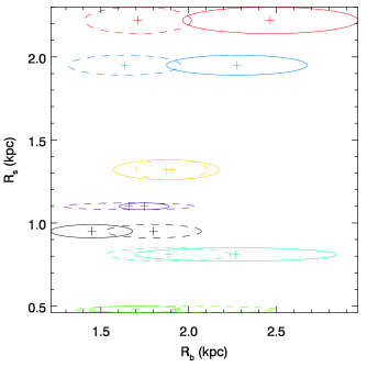
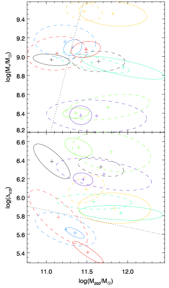
5.5. Lick indices and stellar populations

Our data cover a set of Lick indices that are useful as basic age/metallicity/$\alpha$-abundance indicators in old stellar populations. The recent star formation in these galaxies complicates the straightforward application of simple stellar population models, but we present a simple method to isolate the older stellar populations in our spectra. We then employ a well-known algorithm that inverts indices into stellar population parameters. The absolute values and gradients of such population parameters may provide empirical clues into the physics shaping the dark matter halos.

We have tried using the EZ_AGES software (Graves & Schiavon, 2008) to invert line indices into stellar population parameters. Also provided in this package is LICK_EW, which makes standardized EW measurements on the Lick index system for any observations taken with higher resolution than the original Lick system. We cover the indices H$\beta$ (although not the entire blue Lick sideband; see Appendix E), Fe5015, Mg₁, Mg₂, Mg_b (which is encompassed in the Mg₂ bandpass and therefore not independent), Fe5270, Fe5335, and Fe5406. Often, a more robust combination is quoted as $\langle$Fe$\rangle$, which is the average of Fe5270 and Fe5335. At the heart of EZ_AGES are the stellar population models from Schiavon (2007). The inversion is not simple because at low resolution there are no lines that sample a single element. One simple approximation is to use the combined indices of Thomas et al. (2003) of [MgFe’]=$\sqrt{Mg_{\textrm{b}}\times(0.72\textrm{Fe}5270+0.28\textrm{Fe}5335)}$ as a [Mg/Fe]-independent index and Mg${}_{\textrm{b}}$/$\langle$Fe$\rangle$ as a [Fe/H]-independent index.

For comparing galaxies of different ages, it is better to use the EZ_AGES solution. Our efforts to isolate the indices from old stellar populations and apply EZ_AGES are documented in Appendix E. We cannot find corrections that have valid solutions within EZ_AGES. The indices, particularly H$\beta$ and $\langle$Fe$\rangle$, fall lower than all model grids. Instead, we simply report the two Thomas et al. (2003) indices, with correction factors to isolate the old stellar populations, and warn the reader that the measurements may yet be affected by younger star formation.

The correlations of [MgFe’] and Mg${}_{\textrm{b}}$/$\langle$Fe$\rangle$ with $\gamma$ are shown in Figure 14. Neither shows strong correlation with $\gamma$, but a weak correlation for Mg${}_{\textrm{b}}$/$\langle$Fe$\rangle$ does exist for $\gamma$ based on the stellar models. This is opposite to the trend we would expect from SN feedback. No correlation exists for the gas-measured values of $\gamma$. We present this result with the caveat that since EZ_AGES models cannot fit our data, the Mg${}_{\textrm{b}}$/$\langle$Fe$\rangle$ may also have contamination from unremoved age effects.

Figure 14.— The DM density logarithmic slopes compared to two linear combinations of corrected equivalent widths. The values have been corrected, by a ratio of template values, to isolate the old (3–13 Gyr) populations present for which Lick indices are commonly used. The Lick indices still fall off the EZ_AGES grids after correction, but not by as much. These measurements may help validate or falsify recent SN feedback models, but model predictions for abundances do not yet exist. Stellar-based values are dotted and gas-based values use solid lines. The maximum likelihood linear model fit of the stellar-based values is shown. The confidence interval for [MgFe’] covers nearly the entire plotted range and is not shown. The confidence interval for Mg${}_{\textrm{b}}$/$\langle$Fe$\rangle$ is shown in gray. This is the opposite trend we expect for a SN feedback model. However, rigorous predictions by the modeling groups must be compared to our results before this becomes strong evidence. Further observations are also warranted to reach better statistics. Mg${}_{\textrm{b}}$/$\langle$Fe$\rangle$ may also be affected by uncorrected age effects since the EZ_AGES models cannot match the data. The color coding per galaxy is the same as in Figure 7. The maximum likelihood linear fit to the stellar-based values is shown. Stellar-based values are dotted and gas-based values use solid lines.

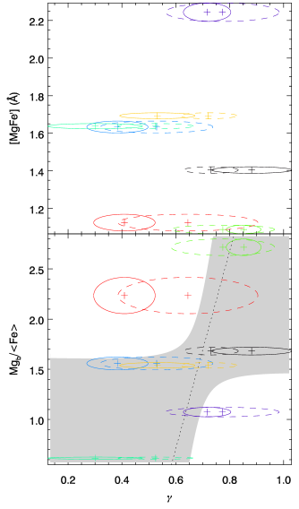
We find one weak correlation of $\gamma$ with chemical structure, but the trend is in an unexpected direction and sensitive to the source of our $\gamma$ measurement. We also do not know how strong the relation between $\gamma$ and chemical abundance patterns is predicted to be from SN feedback models and whether are measurements are unexpected. In the case of a single starburst creating the DM cores, one may expect the most strongly cored galaxies to also be highest in Mg${}_{\textrm{b}}$/$\langle$Fe$\rangle$. However, since the SN feedback models predict repeated bursts of star formation, it may be that the multiple generations of starbursts will wash out the $\alpha$-enhancement from any one short starburst. The answer will depend on how important the last burst is to the luminosity and abundance buildup. We advocate that quantitative abundance predictions be extracted from SN feedback simulations in future works.

6. Conclusions

We have measured the kinematics in seven late-type dwarf galaxies with a wide-field, optical, integral field spectrograph. The gas radial velocities were fit with tilted ring models. The functional forms we explored were one with radial motion and a second for a bar-like potential, We have also measured radial velocities and dispersions for the stars and fit axisymmetric, anisotropic Jeans models to the stellar kinematics. To fully sample the large dimensional parameter spaces, we have made Bayesian parameter estimates with a Markov Chain Monte Carlo program.

We find that generalized Navarro-Frenk-White (gNFW) density profiles adequately describe the kinematic fields. Burkert profiles can also fit most of the sample adequately. The values of the central logarithmic slope of the DM density profile, $\gamma$, we obtain always lie below the value for a pure NFW fit, although not significantly so in some cases. The stellar kinematics likely have different systematics than the gas, and may perhaps be less biased to unmodeled effects such as non-axisymmetric structure. However, we find that the bulk gNFW parameters between the gas-traced and stellar-traced models are usually in good agreement given the uncertainties. This is particularly true for $\gamma$. NGC 2976 has been known to permit an alternate gas-traced solution if a bar is present (Spekkens & Sellwood, 2007). NGC 2976 indeed looks most cored when the gas velocity field is fit with a radial component and more cuspy when either fit with the gas velocity field plus a bar component or fit with the stellar velocity field. The two patches of offset, peaked star formation in NGC 2976 may also signpost a weak bar. NGC 5949 shows 1-$\sigma$ evidence for a cuspier stellar-traced fit, but the two forms of gas-traced fits do not disagree in this case. The remaining five galaxies show no kinematic evidence for bars or biased values of $\gamma$. Even for the two galaxies with a potentially biased $\gamma$, the amplitude of the bias is too small to reconcile the results with a fully cuspy profile. The mean and standard deviation for the sample from the stellar fits are $\gamma=0.67\pm 0.10$.

Finally, we have searched for parameter correlations with $\gamma$ in the hopes of bolstering or rejecting some of the theoretical mechanisms that may core out DM halos. We find weak and likely unimportant correlations of $\gamma$ with vertical orbital anisotropy and DM fraction within 2 disk scale lengths. We measure $\Delta_{V/2}$, a previously used metric for the DM overdensity within the half-maximum velocity region, and we find that $\Delta_{V/2}$ is in line or even higher than recent N-body simulation predictions for cuspy halos. For our galaxies, the core-cusp problem manifests in $\gamma$ but not in $\Delta_{V/2}$. Since these two values are sensitive to masses at somewhat different scales, this result may limit the radial range to which DM mass is getting redistributed. We have looked for a correlation between the core sizes and the stellar disk sizes and found none. Some recent self-interacting DM simulations have predicted such a relation. Finally, we have used the available Lick indices to search for systematic differences in Fe or $\alpha$-abundance. Within the large observational uncertainties, we find no correlations of [MgFe’] with $\gamma$ but a weak correlation with a Lick index combination sensitive to $\alpha$-abundance. This is contrary to our expectations for SN feedback models with bursty star formation histories.

This work builds upon an earlier study where one galaxy was found to give significantly different measurements of $\gamma$ when measured in gas and stars. Our expanded sample size and analysis shows that some biases in traditional gas fits do exist, and that the biases can be explained by bar-like non-axisymmetric structure. However, the amplitude of the biases, when present, appear to be too small to be primarily responsible for the core-cusp problem. While a larger sample is still desirable and is being pursued by members of our group, these results suggest that some mechanism is indeed altering DM halos beyond the physics present in the ordinary $\Lambda$CDM N-body simulations. We have searched for correlations to explicate such a mechanism, and none are yet promising as directions for further research.

Appendix A Composite Kinematic Templates

We have created composite kinematic templates from an empirical database of stellar spectra (Prugniel & Soubiran, 2001). There are two reasons that recommend the composite method. First, the averaging of many stars will reduce the systematics from any non-representative abundances or unusual rotation in a single template stars. Second, the issue of template selection needs to be both flexible and constrained. Abundance, dust, and age gradients may exist, in which case the LOSVD ought to be allowed to select different weights amongst an inclusive template set for each bin. Alternatively, the LOSVD program ought not to have enough freedom to distribute template weights at an extreme level between neighboring bins. The youngest stars that contribute significantly to the integrated light in these galaxies, mostly A stars, have intrinsically broader spectral features than, say, K dwarfs. Allowing one bin to select only A stars and then allowing its neighbor to select only K stars is unphysical. A natural way to accommodate these requirements is to form a small number of composite templates.

The composite templates were constructed by stacking stars from ELODIE (Prugniel & Soubiran, 2001) with weights. The weights were determined by mapping the stars’ T_eff and logg onto isochrones, populating the density along the isochrone according to an initial mass function, and solving for the weights that most accurately reproduced the model population. Similar steps are done by all stellar population synthesis models (e.g. Vazdekis et al., 2003; Bruzual & Charlot, 2003). Let $k$ represent the index of the single-age populations, and f_k represent the mass fraction being put into the isochrone. Along each isochrone $k$ there are tabulated properties at index $j$ for the stellar mass of a bin (m_j,k), the bin size step in mass ($\Delta$m_j,k), the logarithm of the effective temperate ($\log T_{eff,j,k}$), the logarithm of the surface gravity ($\log g_{j,k}$), and the absolute V-band magnitude (M_V,j,k). Let $i$ be the index for the subset of stars selected from ELODIE with m_V,i as the apparent V-band magnitude, $\log T_{eff,i}$ as the logarithm of the effective temperature, $\log g_{i}$ as the logarithm of the surface gravity, $\sigma_{T}$ as the uncertainty on the $\log T_{eff,i}$, and $\sigma_{g}$ as the uncertainty on $\log g_{i}$. The exact values of the uncertainties are unimportant and serve to slightly smooth or sharpen the the stellar weights. We estimate $\sigma_{T}=0.02$ and $\sigma_{g}=0.3$ throughout. Let $m$ be the index for an internal sums run over the ELODIE stars, and let $l_{m,j,k}$ represent the relative likelihood that star $m$ is a good representative for mass bin $j$ according to its $T_{eff}$ and $\log g$ parameters. Finally, let $\xi(m_{j})\Delta m_{j,k}$ represent the number density of stars from the IMF, which is normalized to integrate to one solar mass. With this, we make a composite stack with weight $\eta_{i}$ for the flux-calibrated star $i$ as,

$$-2\ln l_{m,j,k}=\left(\frac{\log T_{eff,m}-\log T_{eff,j,k}}{\sigma_{T}}\right)^{2}$$

$$+\left(\frac{\log g_{m}-\log g_{j,k}}{\sigma_{g}}\right)^{2}$$ (A1)

$$\eta_{i}=\sum_{k}\biggl{(}f_{k}\times\sum_{j}\Bigl{(}10^{\frac{m_{v,i}-M_{v,j,k}}{2.5}}\times\xi(m_{j,k})$$

$$\times\frac{l_{i,j,k}}{\sum_{m}l_{m,j,k}}\times\Delta m_{j,k}\Bigl{)}\biggl{)}.$$ (A2)

In particular, we have used a Chabrier IMF (Chabrier, 2003) and the Padova isochrones (Bressan et al., 2012). The stellar parameters were taken from ELODIE’s TGMET values (Katz et al., 1998). We have used all stars with -1.0$<$[Fe/H]$<$0.2, and stars of any metallicity when T${}_{eff}>$9000K. The metallicity of very hot stars has very little impact on the composite EWs, and the isochrones could not be well populated without the more forgiving criterion. The distribution of stars and the isochrones are shown in Figure 15. Four composites were generated as instantaneous burst models with the following sets of mass-weighted fractions: 100% at 13 Gyr, 50% each of 13 Gyr and 1 Gyr, 50% each of 13 Gyr and 250 Myr, and 50% each of 13 Gyr and 50 Myr. We experimented with additional criteria, such as drawing only -0.3$<$[Fe/H]$<$0.2 stars for the $<$1 Gyr tracks and -1.0$\leq$[Fe/H]$<$-0.3 stars for the $\geq$1 Gyr tracks, but such changes had no measurable impact on our kinematic estimates. The LOSVD software can then determine optimal weights between these four templates. This parametrization constrains any fit to have, at minimum, a 50% mass-weighted fraction in an old population. Templates 1 and 3 take on EWs in Mg${}_{\textrm{b}}$ that are larger and smaller, respectively, than any galaxy regions we observe, meaning that linear combinations of templates can match all the data.

Figure 15.— The ELODIE stars and the Bressan et al. (2012) isochrones selected to generate composite kinematic templates. The four lines correspond to the listed ages for instantaneous burst. The four template spectra in Figure 16 use weighted combinations of these four ages. The datapoints show spectra available for stacking in two metallicity bins. We have tested using the two metallicity bins and found no difference in the extracted kinematics. Our final stacks use [Fe/H] both bins. The oldest isochrones are best populated, but some stars up to the main sequence turnoff are available for all four ages.

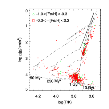
We show the four composite template spectra after normalization in Figure 16.

Figure 16.— Spectra for the four normalized, composite kinematic templates. Template one has a purely old stellar population, and the other three have a contribution from a progressively younger burst as specified in Figure 15. From bottom to top are templates 1–4 with offsets of 0.4. The data are shown in their native R=10,000 resolution. Our stellar kinematic extraction uses these four templates with arbitrarily fitted weights to measure LOSVDs in each bin.

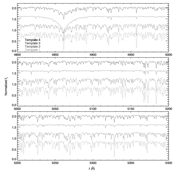
Appendix B MGE DM Halos

While simple equations exist for the circular velocity of a gNFW halo (Dutton et al., 2005), it is more convenient in the JAM framework to approximate the halo in MGE terms. This functionality is available with the IDL MGE_fit_1d routine provided by M. Cappellari, and we have adapted it into FORTRAN for compatibility with our MCMC pipeline. The only change was with the underlying constrained minimization routine. MGE_fit_1d uses MPFIT (Markwardt, 2009) and its underlying MINPACK algorithm (Moré, 1978), while we used a version of conmin (Vanderplaats, 1973) adapted from FORTRAN77 to FORTRAN90. We fit the MGE terms to the gNFW function over physical scales corresponding to one-tenth the size of a fiber and ten times the largest galacto-centric distance of any fiber. On average, 10 MGE terms can reproduce the gNFW function to a maximum density deviation of 5% over this range.

Appendix C Tests on vertical orbital anisotropy

The stellar orbits for the very-late type galaxies in this study are expected to be significantly flattened. Early work, without kinematics, found a large scatter in the orbital anisotropy with a sample of massive spirals from $0.2<\beta_{z}<0.9$ (van der Kruit & de Grijs, 1999). The SAURON project has found that giant, fast-rotator galaxies usually exhibit small, positive $\beta_{z}$ anisotropies (Cappellari et al., 2007). Williams et al. (2009) has extended such studies to S0 systems and confirm that the JAM methods work well on lower mass and diskier systems. More directly relevant to our sample, several works have investigated SVE anisotropies in late-type galaxies by measuring both stellar and gaseous kinematics. These works operate in a cylindrical frame, and require the conditions behind epicycle theory to apply. When this is true and the inclination is known, stellar kinematic measurements along the major and minor axis completely determine the SVE (Shapiro et al., 2003). While the SVE is technically constrained with these measurements, the quality of the constraint depends on location along the rotation curve. Along a linearly-rising portion of a rotation curve, the tangential and radial dispersions are nearly equal, and the dispersion-map will be nearly constant with azimuth angle. More information can come from measuring gas kinematics and using the asymmetric drift equation (Binney & Tremaine, 2008) as an additional constraint. This method, rather than the azimuthal variation, is used by the DiskMass Survey to constrain SVE ratios (Bershady et al., 2010b; Westfall et al., 2011). Most published measurements agree that late-type systems should have very high $\beta_{z}$ anisotropies, approaching the physical limit of $\beta_{z}=1$. Noordermeer et al. (2008) measure NGC 2985 (Hubble-type SAab) to have $\beta_{z}=0.5$. For UGC 463 (Hubble-type SABc), Westfall et al. (2011) find $\beta_{z}=0.8$. Shapiro et al. (2003) measured a trend against a sample of Sa–Sbc galaxies whereby $\beta_{z}$ steadily rose. Gerssen & Shapiro Griffin (2012) continued this work by measuring two later types, NGC 2280 (Hubble-type Scd) and NGC 3810 (Hubble-type Sc), and found $\beta_{z}=0.94$ and $\beta_{z}=0.92$, respectively. These two measurements continued the trend fit to the earlier-type galaxies (Figure 4 of Gerssen & Shapiro Griffin (2012)). While it may be reasonable to set a prior on $\beta_{z}$ peaked at large values, we found that some of our data are poorly represented by large orbital anisotropies. Therefore, we have selected a flat prior on $\beta_{z}$. Of course orbital anisotropy can also be measured by using higher order velocity moments, but this is not possible at our S/N and instrumental velocity resolution.

Readers familiar with mass modeling of giant elliptical galaxies may expect a strong negative covariance between the estimation of orbital anisotropy and $\gamma$. For instance, van der Marel (1994) made models of M87 for a range of orbital anisotropies, $\beta$, in his Figure 10. Models with large $\beta$ have higher central dispersions. However, it is important to remember that the M87 model is in a spherical coordinate frame with $\sigma_{\phi}=\sigma_{\theta}$, and so large values of $\beta$ only have radial dispersion support. Alternatively, with disky galaxies in a cylindrical frame, the ratio of radial and tangential dispersions is set by the Jeans equations and stay of order unity near the center. Therefore, even when $\beta_{z}$ is near unity in a disky system, $\beta$ will be significantly softened and not approach unity. We have made a numerical test on our ability to measure $\beta_{z}$ and de-couple it from $\gamma$ as follows. A model realization was generated from a set of parameters with $\beta_{z}$ values ranging from -0.8–0.8 in the bin positions of the NGC 2976 observations. The remaining parameters were set as $\left\{\log M_{200},c,\gamma,\Upsilon_{*},i,PA,v_{sys},\Delta\alpha_{o},\Delta\delta_{0},\sigma_{sys}\right\}=\left\{11.3,15.0,0.4,0.7,62.0,-36.0,6.0,0.0,0.0,5.0\right\}$. The JAM models only predict the second-moment velocity, $v_{rms}^{2}$, while we need both $v_{los}$ and $\sigma$ in order to include v_sys in our fitting process. Following the JAM formalism (Cappellari, 2008), we have used the parameter

$$\kappa_{k}\equiv\frac{\left[\overline{v_{\phi}}\right]}{\left(\left[\overline{v^{2}_{\phi}}\right]-\left[\overline{v^{2}_{R}}\right]\right)^{1/2}}$$ (C1)

to divide the second-moment tangential velocity into rotation and dispersion. The line-of-sight first-moment velocity can then be calculated by Equation 38 of Cappellari (2008) through a double numerical integration. For this exercise, we have set $\kappa_{k}=0.7$. $\kappa_{k}=0.0$ gives a non-rotating system and $\kappa_{k}=1.0$ makes the radial and tangential dispersion equal. Since the actual fit is still to the second-moment velocity, the choice of $\kappa$ is unimportant. We then fit the simulated data with our MCMC pipeline. The original NGC 2976 bins and uncertainties were used in the likelihood fit. The second-moment velocity fields for two anisotropies, representing an isotropic field and the largely anisotropic values that previous studies have found, are shown in Figure 17. JAM models with even larger orbital anisotropies ($\beta_{z}=0.8$) become so extreme that the second-moment velocities peak in the middle. The MCMC fits do not perfectly converge on the input model for the most vertically biased models, but over the most likely range (positive $\beta_{z}$) the residuals are consistent with the level of observational uncertainty used in the simulations. We highlight several important points from this figure. First, the orbital anisotropy can, with limited precision, be inferred from our data in Figure 18. When galaxies have truly large vertical orbital anisotropies ($\beta_{z}>0.5$), we find them in our MCMC analysis. Second, there is very little covariance between $\beta_{z}$ and $\gamma$. The more important covariances are between $\Upsilon_{*}$, $c$, $M_{200}$, and $\gamma$. Our results on the DM density profiles are largely independent of our results on the orbital anisotropy. Finally, we do not consistently find the large orbital anisotropies (in §3.2) that other groups have with similar data and systems. The reason for this potential discrepancy is not known, but we will propose some possibilities in §5.

Figure 17.— Second-moment velocity fields simulated with JAM for a simple parameter set. Noise equal to that in the data has been added. Two values for the orbital anisotropy are shown: a low one that represents most of our data and a higher one as has been found by earlier studies. More flattened velocity ellipsoids generate larger dispersions at small radii. Steeper DM profiles will also generate larger second-moment velocities at small radii. The full velocity map is less degenerate between $\beta_{z}$ and $\gamma$ than a single position-velocity cut. Top $\beta_{z}=0.0$. Bottom $\beta_{z}=0.6$. The difference between the two is visible by eye, and our simulations can recover $\beta_{z}$ and $\gamma$ with little degeneracy.

Figure 18.— Residuals of the extracted parameters from simulated data with a range of input orbital anisotropies. The data sampling and S/N ratios were the same as for the NGC 959 data. The error bars indicate the 68% confidence interval from MCMC samples. The residuals for the parameters other than $\beta_{z}$ do not show a correlation with the true $\beta_{z}$. For the most negative $\beta_{z}$ values, the MCMC estimate returns a value significantly higher than the correct one, but the estimate becomes more accurate for the more plausible range of $\beta_{z}>0$ as found in real galaxies. The reason may be that the walkers are initialized on the positive end of $\beta_{z}$. We are mainly concerned that $\gamma$ does not show a bias in these simulations.

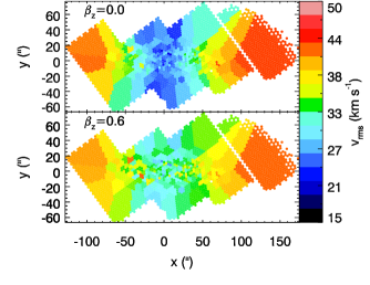
Appendix D Tests on MCMC convergence

Three parameters in emcee mainly determine whether the parameter space has been fully sampled and all minima have been found: the number of “walkers”, the length of “burn-in”, and the number of samples kept per walker. The number of walkers is suggested by the emcee documentation to be at least twice the number of parameter dimensions, but walkers numbering an order of magnitude more than the problem dimensionality are more common. Some number of the early MCMC samples are likely to represent the initialization choices rather than the underlying probability distribution. Usually, a number of these first samples are ignored in a “burn-in” phase. Lastly, the number of samples in the MCMC chain kept determine the resolution quality to the fit. We have set the number of burn-ins and the number of kept samples at 20 and 250 for each walker. A simple convergence test was run by varying the number of walkers on simulated kinematic data sets. The data were simulated for the NGC 959 footprint and S/N with parameters $\left\{\log M_{200},c,\gamma,\beta_{z},\Upsilon_{*},i,PA,v_{sys},\Delta\alpha_{o},\Delta\delta_{0}\right\}=\left\{11.3,15.0,0.4,0.3,0.7,55.2,67.9,595.0,0.0,0.0\right\}$. Five independent realizations were made by drawing normally distributed errors for both the gaseous and stellar kinematic fields. Each field was analyzed with 50, 100, 150, 250, and 400 walkers. The central estimates and dispersions of all parameters did not change for solutions with $>$100 walkers. We conservatively chose 250 walkers for our final fits.

The recovered parameters show several useful trends. First, some parameters, such as $c$, $\gamma$, $\Upsilon_{*}$, $i$, and $PA$ show slightly more scatter when using only 50 walkers. Along with the number of walkers, the total number of samples is decreased. The increased scatter means that we have not reached complete convergence in the MCMC fit. The scatter and bias stay flat for all simulations with more than 50 walkers. The remaining scatter at larger walker numbers represents the limited S/N in the observations. As a conservative choice, we have selected 250 walkers for all the fits to real data. Second, we see that several parameters have slight biases from their true values. We have selected the simulation to have some parameters offset from the prior peaks and the posterior probabilities are being influenced by the priors for M₂₀₀ and $\Upsilon_{*}$. $i$ shows a small bias because of the asymmetric limits required by the MGE terms. For these three variables, the biases are still quite small.

Appendix E Age Corrections for Lick Indices

EZ_AGES operates by iteratively solving for age, [Fe/H], and [$\alpha$/Fe] by interpolating index measurements to the Schiavon (2007) stellar population grids. For our wavelengths of interest, H$\beta$ and $\langle$Fe$\rangle$ are first selected as relatively clean indicators of age and [Fe/H]. EZ_AGES matches these two index measurements to the grids with the remaining elements fixed. EZ_AGES can use either a solar scaled grid or an $\alpha$-enhanced grid (Salasnich et al., 2000). Using the Large Magellanic Cloud (LMC) as a proxy for our galaxies, the [$\alpha$/Fe] values of individual stars (Johnson et al., 2006; Mucciarelli et al., 2008; Pompéia et al., 2008) and star clusters (Colucci et al., 2012) are at solar values until [Fe/H]$<$-1 and less $\alpha$-enhanced than Milky Way stars at fixed [Fe/H]. We have tried both options but found the same results with both. EZ_AGES then selects indices that are sensitive to other elements. In our case, the relevant index is Mg_b and the relevant abundance is [Mg/Fe]. EZ_AGES re-estimates age and [Fe/H] in the H$\beta$-Mg_b plane. If the estimates differ, primarily in estimated [Fe/H], the parameter [Mg/Fe] is adjusted until the two [Fe/H] estimates agree. There are no good indicators of [O/Fe] at low resolution, so we have adopted the default assumption of [O/Fe]=0.0. We have also let the other important $\alpha$-elements, Na, Si, and Ti, track Mg. LICK_EW propagates observational uncertainties in the spectrum into Lick index uncertainties, and EZ_AGES further propagates these into stellar population parameter uncertainties. Graves & Schiavon (2008) provide tests on globular cluster data with higher resolution spectroscopy and validate their accuracy to 0.15 dex in age and 0.1-0.2 dex in [Fe/H] and [Mg/Fe]. They also compare parameters estimated for a galaxy sample (Thomas et al., 2005) that has been studied with an earlier inversion technique (Thomas et al., 2003). Some small zeropoint offsets are found, but the two methods generally agree. This algorithm has recently been employed by a group studying population gradients in the far outskirts of nearby elliptical galaxies (Greene et al., 2012, 2013) using IFU data similar to ours.

We first must make a correction for the H$\beta$ index and our limited spectral coverage. To optimize the S/N at Mg$b$, we set up the grism so that the full range of the H$\beta$ was not recorded. The lowest wavelength that all our observing runs covered, including a 5Å buffer, is 4855Å, which misses the entire blue sideband and some of the main index window. The core of H$\beta$ is retained in our window. However, the kinematic templates we use cover this whole range and do well to approximate the observed spectra. We therefore measure the EW of a narrower index in both our data and the matching template-based kinematic model, and then the full H$\beta$ index in the template-based kinematic model. Let nH$\beta$ be this narrower H$\beta$ index, with a bandpass of 4857.000–4876.625Å and sidebands from 4855.300–4857.000Å and 4876.623–4891.600Å. The index is measured inside the LICK_EW package. We form the corrected measurement as,

$$H\beta=\frac{H\beta(model)\times nH\beta(data)}{nH\beta(model)}.$$ (E1)

An important complication facing us is that our sample galaxies are not well represented as old, simple stellar populations. EZ_AGES performs best, with minimal zeropoint uncertainty, for very old ($>$10 Gyr) populations. Furthermore, the Schiavon (2007) grids are limited to 1–15 Gyr ages and -1.3$<$[Fe/H]$<$0.3. However, we do have some information on the separation of old and young stellar populations by the nature of our LOSVD template selection. We will leverage the kinematic template weights and measurements of Lick indices on the composite templates to approximate the Lick indices of the old stellar populations. We give the Lick indices and the narrow H$\beta$ as measured off the four kinematic templates in Table 9.

Table 9Index measurements for the kinematic templates.

Template	H$\beta$	nH$\beta$	Fe5015	Mg1	Mg2	Mg${}_{\textrm{b}}$	Fe5270	Fe5335	Fe5406
	(Å)	(Å)	(Å)	(mag)	(mag)	(Å)	(Å)	(Å)	(Å)
1	1.71	0.72	5.03	0.0068	0.0847	2.82	3.09	2.59	1.73
2	3.50	1.08	3.74	0.0022	0.0527	1.65	2.10	1.75	1.05
3	7.65	2.26	1.22	-0.0007	0.0200	0.64	0.69	0.59	0.45
4	3.80	1.00	2.33	-0.0026	0.0118	0.25	0.84	0.83	0.40

Table 10Luminosity weight of 13 Gyr population in each composite template.

Template	lw(H$\beta$)	lw(nH$\beta$)	lw(Fe5015)	lw(Mg1)	lw(Mg2)	lw(Mgb)	lw(Fe5270)	lw(Fe5335)	lw(Fe5406)
2	0.133	0.160	0.083	0.129	0.106	0.114	0.127	0.148	0.134
3	0.028	0.036	0.016	0.087	0.034	0.027	0.036	0.031	0.037
4	0.000	0.021	0.010	0.036	0.000	0.007	0.014	0.019	0.009

It is impossible to find valid solutions in EZ_AGES for the directly measured Lick indices. Stellar populations younger than those in the model libraries suppress the Fe and Mg line strengths to values that fall off all available grids. We make a crude recovery of the old population indices as follows. In its most general form, the equivalent width of a composite population cannot be expressed as a linear combination of its component equivalent widths. However, when the continua of the populations only vary slowly over the index bandpass, such an equation is approximately correct. Let EW_t be the total equivalent width, EW_i be the equivalent width of the component populations in a particular index, $f_{\lambda,i}$ be the flux density, $f_{\lambda,c,i}$ be the continuum flux density, $\overline{f_{\lambda,c,i}}$ be the average flux density over the index bandpass, and f_i be the normalized luminosity weight of component $i$ as found during the LOSVD fit. Then,

$$EW_{t} \equiv\int(1-\frac{\sum_{i}f_{i}f_{\lambda,i}}{\sum_{i}f_{i}f_{\lambda,c,i}})d\lambda$$

$$\approx\frac{\sum_{i}f_{i}EW_{i}\overline{f_{\lambda,c,i}}}{\sum_{i}f_{i}\overline{f_{\lambda,c,i}}}.$$ (E2)

The ELODIE templates may not accurately represent the stellar population parameters contained in our target galaxies. As such, their absolute equivalent widths should not be used. We instead form a correction to the measured equivalent widths by the ratio of the old population template and the total template equivalent widths. We count both the 13 and 3 Gyr populations as old, as EZ_AGES has models that bracket both, and form the following corrected ratio for each atomic-type equivalent width. Since the kinematic templates are continuum normalized, the average continua fall out of the equation. Let lw_i,j be the luminosity weight of the 13 Gyr population in index j of template i (with lw$\equiv$1 for i$=1$) from Table 10, $\mu_{i}$ be the LOSVD-measured template weight, and tEW_i,j be the template’s equivalent width from Table 9. We form corrected equivalent widths, EW_j, from the directly measured values, mEW_j, as

$$EW_{j}=mEW_{j}\times$$

$$\frac{\sum_{i=1,2}\mu_{i}tEW_{i,j}+\sum_{i=3,4}\mu_{i}lw_{i,j}tEW_{i,j}}{(\sum_{i=1,2}\mu_{i}+\sum_{i=3,4}\mu_{i}lw_{i,j})\times(\sum_{i}\mu_{i}tEW_{i,j})}.$$ (E3)

Mg₁ and Mg₂ are molecular-type equivalent widths with units of magnitudes, and we measure their values by first transforming the magnitudes into linear units, applying the linear correction, and then transforming back into magnitudes. The S/N of the index measurements in individual fibers or even the kinematic bins are too noisy to be useful. So, we have made one bin per galaxy. The two most common ways that the data fall off EZ_AGES grids is that H$\beta$ is too low or $\langle$Fe$\rangle$ is too low. If we average all the data and push H$\beta$ up onto the grid to the location of a 10 Gyr age, we find [Fe/H]$\sim$-1 and [Mg/Fe]$\sim$0.5. This value of [Mg/Fe] is surprisingly high considering the values measured for the LMC. The uncorrected values also fall off the grids, but with Mg${}_{\textrm{b}}$ and often $\langle$Fe$\rangle$ that are too small for the lowest abundance models.

References

- Abazajian et al. (2001) Abazajian, K., Fuller, G. M., & Patel, M. 2001, Phys. Rev. D, 64, 023501
- Adams et al. (2011) Adams, J. J., Blanc, G. A., Hill, G. J., et al. 2011, ApJS, 192, 5
- Adams et al. (2012) Adams, J. J., Gebhardt, K., Blanc, G. A., et al. 2012, ApJ, 745, 92
- Alam et al. (2002) Alam, S. M. K., Bullock, J. S., & Weinberg, D. H. 2002, ApJ, 572, 34
- Amorisco et al. (2013a) Amorisco, N. C., Agnello, A., & Evans, N. W. 2013a, MNRAS, 429, L89
- Amorisco & Evans (2012) Amorisco, N. C., & Evans, N. W. 2012, MNRAS, 419, 184
- Amorisco et al. (2013b) Amorisco, N. C., Zavala, J., & de Boer, T. J. L. 2013b, ArXiv e-prints
- Avila-Reese et al. (2001) Avila-Reese, V., Colín, P., Valenzuela, O., D’Onghia, E., & Firmani, C. 2001, ApJ, 559, 516
- Bagetakos et al. (2011) Bagetakos, I., Brinks, E., Walter, F., et al. 2011, AJ, 141, 23
- Barnabè et al. (2012) Barnabè, M., Dutton, A. A., Marshall, P. J., et al. 2012, MNRAS, 423, 1073
- Behroozi et al. (2013) Behroozi, P. S., Wechsler, R. H., & Conroy, C. 2013, ApJ, 770, 57
- Bell & de Jong (2001) Bell, E. F., & de Jong, R. S. 2001, ApJ, 550, 212
- Bershady et al. (2011) Bershady, M. A., Martinsson, T. P. K., Verheijen, M. A. W., Westfall, K. B., Andersen, D. R., & Swaters, R. A. 2011, ApJ, 739, L47+
- Bershady et al. (2010a) Bershady, M. A., Verheijen, M. A. W., Swaters, R. A., et al. 2010a, ApJ, 716, 198
- Bershady et al. (2010b) Bershady, M. A., Verheijen, M. A. W., Westfall, K. B., et al. 2010b, ApJ, 716, 234
- Bertin & Arnouts (1996) Bertin, E., & Arnouts, S. 1996, A&AS, 117, 393
- Bertin et al. (2002) Bertin, E., Mellier, Y., Radovich, M., et al. 2002, in Astronomical Society of the Pacific Conference Series, Vol. 281, Astronomical Data Analysis Software and Systems XI, ed. D. A. Bohlender, D. Durand, & T. H. Handley, 228
- Binney & Tremaine (2008) Binney, J., & Tremaine, S. 2008, Galactic Dynamics: Second Edition (Princeton University Press)
- Blais-Ouellette et al. (2001) Blais-Ouellette, S., Amram, P., & Carignan, C. 2001, AJ, 121, 1952
- Blais-Ouellette et al. (2004) Blais-Ouellette, S., Amram, P., Carignan, C., & Swaters, R. 2004, A&A, 420, 147
- Blanton & Roweis (2007) Blanton, M. R., & Roweis, S. 2007, AJ, 133, 734
- Blumenthal et al. (1986) Blumenthal, G. R., Faber, S. M., Flores, R., & Primack, J. R. 1986, ApJ, 301, 27
- Bosma (1978) Bosma, A. 1978, PhD thesis, PhD Thesis, Groningen Univ., (1978)
- Bosma (1981a) —. 1981a, AJ, 86, 1791
- Bosma (1981b) —. 1981b, AJ, 86, 1825
- Breddels et al. (2013) Breddels, M. A., Helmi, A., van den Bosch, R. C. E., et al. 2013, MNRAS, 433, 3173
- Bressan et al. (2012) Bressan, A., Marigo, P., Girardi, L., et al. 2012, MNRAS, 427, 127
- Bruzual & Charlot (2003) Bruzual, G., & Charlot, S. 2003, MNRAS, 344, 1000
- Burkert (1995) Burkert, A. 1995, ApJ, 447, L25
- Cappellari (2002) Cappellari, M. 2002, MNRAS, 333, 400
- Cappellari (2008) —. 2008, MNRAS, 390, 71
- Cappellari & Copin (2003) Cappellari, M., & Copin, Y. 2003, MNRAS, 342, 345
- Cappellari et al. (2007) Cappellari, M., Emsellem, E., Bacon, R., et al. 2007, MNRAS, 379, 418
- Carignan et al. (1988) Carignan, C., Sancisi, R., & van Albada, T. S. 1988, AJ, 95, 37
- Cembranos et al. (2005) Cembranos, J. A. R., Feng, J. L., Rajaraman, A., & Takayama, F. 2005, Physical Review Letters, 95, 181301
- Chabrier (2003) Chabrier, G. 2003, PASP, 115, 763
- Colucci et al. (2012) Colucci, J. E., Bernstein, R. A., Cameron, S. A., & McWilliam, A. 2012, ApJ, 746, 29
- Dalcanton & Stilp (2010) Dalcanton, J. J., & Stilp, A. M. 2010, ApJ, 721, 547
- de Blok & Bosma (2002) de Blok, W. J. G., & Bosma, A. 2002, A&A, 385, 816
- de Blok et al. (2003) de Blok, W. J. G., Bosma, A., & McGaugh, S. 2003, MNRAS, 340, 657
- de Blok & McGaugh (1997) de Blok, W. J. G., & McGaugh, S. S. 1997, MNRAS, 290, 533
- de Blok et al. (2001a) de Blok, W. J. G., McGaugh, S. S., Bosma, A., & Rubin, V. C. 2001a, ApJ, 552, L23
- de Blok et al. (2001b) de Blok, W. J. G., McGaugh, S. S., & Rubin, V. C. 2001b, AJ, 122, 2396
- de Blok et al. (1996) de Blok, W. J. G., McGaugh, S. S., & van der Hulst, J. M. 1996, MNRAS, 283, 18
- de Blok et al. (2008) de Blok, W. J. G., Walter, F., Brinks, E., Trachternach, C., Oh, S., & Kennicutt, R. C. 2008, AJ, 136, 2648
- de Vaucouleurs et al. (1991) de Vaucouleurs, G., de Vaucouleurs, A., Corwin, Jr., H. G., et al. 1991, Third Reference Catalogue of Bright Galaxies
- Di Cintio et al. (2014) Di Cintio, A., Brook, C. B., Macciò, A. V., et al. 2014, MNRAS, 437, 415
- Dierckx (1993) Dierckx, P. 1993, Curve and surface fitting with splines (Monographs on Numerical Analysis, Oxford: Clarendon, —c1993)
- Donato et al. (2009) Donato, F., Gentile, G., Salucci, P., et al. 2009, MNRAS, 397, 1169
- Dubinski et al. (2009) Dubinski, J., Berentzen, I., & Shlosman, I. 2009, ApJ, 697, 293
- Dutton et al. (2005) Dutton, A. A., Courteau, S., de Jong, R., & Carignan, C. 2005, ApJ, 619, 218
- Dutton & van den Bosch (2009) Dutton, A. A., & van den Bosch, F. C. 2009, MNRAS, 396, 141
- Dutton et al. (2007) Dutton, A. A., van den Bosch, F. C., Dekel, A., & Courteau, S. 2007, ApJ, 654, 27
- Einasto (1965) Einasto, J. 1965, Trudy Astrofizicheskogo Instituta Alma-Ata, 5, 87
- El-Zant et al. (2001) El-Zant, A., Shlosman, I., & Hoffman, Y. 2001, ApJ, 560, 636
- Emsellem et al. (1994) Emsellem, E., Monnet, G., & Bacon, R. 1994, A&A, 285, 723
- Fabricius et al. (2008) Fabricius, M. H., Barnes, S., Bender, R., et al. 2008, in Presented at the Society of Photo-Optical Instrumentation Engineers (SPIE) Conference, Vol. 7014, Society of Photo-Optical Instrumentation Engineers (SPIE) Conference Series
- Fabricius et al. (2012) Fabricius, M. H., Grupp, F., Bender, R., et al. 2012, in Society of Photo-Optical Instrumentation Engineers (SPIE) Conference Series, Vol. 8446, Society of Photo-Optical Instrumentation Engineers (SPIE) Conference Series
- Favati et al. (1991) Favati, P., Lotti, G., & Romani, F. 1991, ACM Trans. Math. Softw., 17, 218
- Ferrero et al. (2012) Ferrero, I., Abadi, M. G., Navarro, J. F., Sales, L. V., & Gurovich, S. 2012, MNRAS, 425, 2817
- Flores & Primack (1994) Flores, R. A., & Primack, J. R. 1994, ApJ, 427, L1
- Foreman-Mackey et al. (2013) Foreman-Mackey, D., Hogg, D. W., Lang, D., & Goodman, J. 2013, PASP, 125, 306
- Freeman (1970) Freeman, K. C. 1970, ApJ, 160, 811
- Gebhardt et al. (2000) Gebhardt, K., Richstone, D., Kormendy, J., et al. 2000, AJ, 119, 1157
- Gentile et al. (2005) Gentile, G., Burkert, A., Salucci, P., Klein, U., & Walter, F. 2005, ApJ, 634, L145
- Gentile et al. (2004) Gentile, G., Salucci, P., Klein, U., Vergani, D., & Kalberla, P. 2004, MNRAS, 351, 903
- Gerssen & Shapiro Griffin (2012) Gerssen, J., & Shapiro Griffin, K. 2012, MNRAS, 423, 2726
- Governato et al. (2010) Governato, F., Brook, C., Mayer, L., Brooks, A., Rhee, G., Wadsley, J., Jonsson, P., Willman, B., Stinson, G., Quinn, T., & Madau, P. 2010, Nature, 463, 203
- Governato et al. (2012) Governato, F., Zolotov, A., Pontzen, A., et al. 2012, MNRAS, 422, 1231
- Graves & Schiavon (2008) Graves, G. J., & Schiavon, R. P. 2008, ApJS, 177, 446
- Greene et al. (2012) Greene, J. E., Murphy, J. D., Comerford, J. M., et al. 2012, ApJ, 750, 32
- Greene et al. (2013) Greene, J. E., Murphy, J. D., Graves, G. J., et al. 2013, ApJ, 776, 64
- Guo et al. (2011) Guo, Q., White, S., Boylan-Kolchin, M., et al. 2011, MNRAS, 413, 101
- Hernquist (1990) Hernquist, L. 1990, ApJ, 356, 359
- Herrmann & Ciardullo (2009) Herrmann, K. A., & Ciardullo, R. 2009, ApJ, 705, 1686
- Hill et al. (2004) Hill, G. J., Gebhardt, K., Komatsu, E., & MacQueen, P. J. 2004, in American Institute of Physics Conference Series, Vol. 743, The New Cosmology: Conference on Strings and Cosmology, ed. R. E. Allen, D. V. Nanopoulos, & C. N. Pope, 224–233
- Hill et al. (2008b) Hill, G. J., MacQueen, P. J., Smith, M. P., et al. 2008b, in Society of Photo-Optical Instrumentation Engineers (SPIE) Conference Series, Vol. 7014, 231
- Hogan & Dalcanton (2000) Hogan, C. J., & Dalcanton, J. J. 2000, Phys. Rev. D, 62, 063511
- Hogg et al. (2010) Hogg, D. W., Bovy, J., & Lang, D. 2010, ArXiv e-prints
- Holley-Bockelmann et al. (2005) Holley-Bockelmann, K., Weinberg, M., & Katz, N. 2005, MNRAS, 363, 991
- Jardel & Gebhardt (2012) Jardel, J. R., & Gebhardt, K. 2012, ApJ, 746, 89
- Jardel et al. (2013) Jardel, J. R., Gebhardt, K., Fabricius, M. H., et al. 2013, ApJ, 763, 91
- Johnson et al. (2006) Johnson, J. A., Ivans, I. I., & Stetson, P. B. 2006, ApJ, 640, 801
- Kaplinghat (2005) Kaplinghat, M. 2005, Phys. Rev. D, 72, 063510
- Kaplinghat et al. (2013) Kaplinghat, M., Keeley, R. E., Linden, T., & Yu, H.-B. 2013, ArXiv e-prints
- Kaplinghat et al. (2000) Kaplinghat, M., Knox, L., & Turner, M. S. 2000, Physical Review Letters, 85, 3335
- Katz et al. (1998) Katz, D., Soubiran, C., Cayrel, R., Adda, M., & Cautain, R. 1998, A&A, 338, 151
- Kelson (2003) Kelson, D. D. 2003, PASP, 115, 688
- Klypin et al. (2001) Klypin, A., Kravtsov, A. V., Bullock, J. S., & Primack, J. R. 2001, ApJ, 554, 903
- Klypin et al. (2011) Klypin, A. A., Trujillo-Gomez, S., & Primack, J. 2011, ApJ, 740, 102
- Komatsu et al. (2011) Komatsu, E., Smith, K. M., Dunkley, J., et al. 2011, ApJS, 192, 18
- Kowalczyk et al. (2013) Kowalczyk, K., Łokas, E. L., Kazantzidis, S., & Mayer, L. 2013, MNRAS, 431, 2796
- Kregel et al. (2002) Kregel, M., van der Kruit, P. C., & de Grijs, R. 2002, MNRAS, 334, 646
- Kuzio de Naray et al. (2010) Kuzio de Naray, R., Martinez, G. D., Bullock, J. S., & Kaplinghat, M. 2010, ApJ, 710, L161
- Kuzio de Naray et al. (2008) Kuzio de Naray, R., McGaugh, S. S., & de Blok, W. J. G. 2008, ApJ, 676, 920
- Kuzio de Naray et al. (2006) Kuzio de Naray, R., McGaugh, S. S., de Blok, W. J. G., & Bosma, A. 2006, ApJS, 165, 461
- Kuzio de Naray et al. (2009) Kuzio de Naray, R., McGaugh, S. S., & Mihos, J. C. 2009, ApJ, 692, 1321
- Leroy et al. (2008) Leroy, A. K., Walter, F., Brinks, E., et al. 2008, AJ, 136, 2782
- Macciò et al. (2012a) Macciò, A. V., Paduroiu, S., Anderhalden, D., Schneider, A., & Moore, B. 2012a, MNRAS, 424, 1105
- Macciò et al. (2012b) Macciò, A. V., Stinson, G., Brook, C. B., et al. 2012b, ApJ, 744, L9
- Madsen & Gaensler (2013) Madsen, G. J., & Gaensler, B. M. 2013, ArXiv e-prints
- Marchesini et al. (2002) Marchesini, D., D’Onghia, E., Chincarini, G., et al. 2002, ApJ, 575, 801
- Markwardt (2009) Markwardt, C. B. 2009, in Astronomical Society of the Pacific Conference Series, Vol. 411, Astronomical Data Analysis Software and Systems XVIII, ed. D. A. Bohlender, D. Durand, & P. Dowler, 251
- McGaugh et al. (2001) McGaugh, S. S., Rubin, V. C., & de Blok, W. J. G. 2001, AJ, 122, 2381
- McMillan & Dehnen (2005) McMillan, P. J., & Dehnen, W. 2005, MNRAS, 363, 1205
- Milgrom (1983) Milgrom, M. 1983, ApJ, 270, 365
- Monet et al. (2003) Monet, D. G., Levine, S. E., Canzian, B., et al. 2003, AJ, 125, 984
- Monnet et al. (1992) Monnet, G., Bacon, R., & Emsellem, E. 1992, A&A, 253, 366
- Moore (1994) Moore, B. 1994, Nature, 370, 629
- Moré (1978) Moré, J. J. 1978, in Lecture Notes in Mathematics, Vol. 630, Numerical Analysis, ed. G. Watson (Springer Berlin Heidelberg), 105–116
- Mucciarelli et al. (2008) Mucciarelli, A., Carretta, E., Origlia, L., & Ferraro, F. R. 2008, AJ, 136, 375
- Navarro et al. (1996a) Navarro, J. F., Eke, V. R., & Frenk, C. S. 1996a, MNRAS, 283, L72
- Navarro et al. (1996b) Navarro, J. F., Frenk, C. S., & White, S. D. M. 1996b, ApJ, 462, 563
- Navarro et al. (2004) Navarro, J. F., Hayashi, E., Power, C., et al. 2004, MNRAS, 349, 1039
- Navarro et al. (2010) Navarro, J. F., Ludlow, A., Springel, V., et al. 2010, MNRAS, 402, 21
- Newman et al. (2013a) Newman, A. B., Treu, T., Ellis, R. S., & Sand, D. J. 2013a, ApJ, 765, 25
- Newman et al. (2013b) Newman, A. B., Treu, T., Ellis, R. S., et al. 2013b, ApJ, 765, 24
- Noordermeer et al. (2008) Noordermeer, E., Merrifield, M. R., & Aragón-Salamanca, A. 2008, MNRAS, 388, 1381
- Oh et al. (2008) Oh, S., de Blok, W. J. G., Walter, F., Brinks, E., & Kennicutt, R. C. 2008, AJ, 136, 2761
- Oh et al. (2011a) Oh, S.-H., Brook, C., Governato, F., et al. 2011a, AJ, 142, 24
- Oh et al. (2011b) Oh, S.-H., de Blok, W. J. G., Brinks, E., et al. 2011b, AJ, 141, 193
- Paturel et al. (2003) Paturel, G., Petit, C., Prugniel, P., et al. 2003, A&A, 412, 45
- Peter et al. (2013) Peter, A. H. G., Rocha, M., Bullock, J. S., & Kaplinghat, M. 2013, MNRAS, 430, 105
- Pompéia et al. (2008) Pompéia, L., Hill, V., Spite, M., et al. 2008, A&A, 480, 379
- Pontzen & Governato (2012) Pontzen, A., & Governato, F. 2012, MNRAS, 421, 3464
- Portinari et al. (2004) Portinari, L., Sommer-Larsen, J., & Tantalo, R. 2004, MNRAS, 347, 691
- Press et al. (1992) Press, W. H., Teukolsky, S. A., Vetterling, W. T., & Flannery, B. P. 1992, Numerical recipes in FORTRAN. The art of scientific computing
- Prugniel & Soubiran (2001) Prugniel, P., & Soubiran, C. 2001, A&A, 369, 1048
- Rhee et al. (2004) Rhee, G., Valenzuela, O., Klypin, A., Holtzman, J., & Moorthy, B. 2004, ApJ, 617, 1059
- Richardson & Fairbairn (2014) Richardson, T., & Fairbairn, M. 2014, ArXiv e-prints
- Roberts & Whitehurst (1975) Roberts, M. S., & Whitehurst, R. N. 1975, ApJ, 201, 327
- Rocha et al. (2013) Rocha, M., Peter, A. H. G., Bullock, J. S., et al. 2013, MNRAS, 430, 81
- Rubin & Ford (1970) Rubin, V. C., & Ford, Jr., W. K. 1970, ApJ, 159, 379
- Rubin et al. (1978a) Rubin, V. C., Ford, Jr., W. K., Strom, K. M., Strom, S. E., & Romanishin, W. 1978a, ApJ, 224, 782
- Rubin et al. (1980) Rubin, V. C., Ford, W. K. J., & . Thonnard, N. 1980, ApJ, 238, 471
- Rubin et al. (1978b) Rubin, V. C., Thonnard, N., & Ford, Jr., W. K. 1978b, ApJ, 225, L107
- Salasnich et al. (2000) Salasnich, B., Girardi, L., Weiss, A., & Chiosi, C. 2000, A&A, 361, 1023
- Sand et al. (2002) Sand, D. J., Treu, T., & Ellis, R. S. 2002, ApJ, 574, L129
- Sand et al. (2004) Sand, D. J., Treu, T., Smith, G. P., & Ellis, R. S. 2004, ApJ, 604, 88
- Schiavon (2007) Schiavon, R. P. 2007, ApJS, 171, 146
- Schoenmakers et al. (1997) Schoenmakers, R. H. M., Franx, M., & de Zeeuw, P. T. 1997, MNRAS, 292, 349
- Sellwood (2003) Sellwood, J. A. 2003, ApJ, 587, 638
- Sellwood (2008) —. 2008, ApJ, 679, 379
- Sellwood & Sánchez (2010) Sellwood, J. A., & Sánchez, R. Z. 2010, MNRAS, 404, 1733
- Shapiro et al. (2003) Shapiro, K. L., Gerssen, J., & van der Marel, R. P. 2003, AJ, 126, 2707
- Simon et al. (2003) Simon, J. D., Bolatto, A. D., Leroy, A., & Blitz, L. 2003, ApJ, 596, 957
- Simon et al. (2005) Simon, J. D., Bolatto, A. D., Leroy, A., Blitz, L., & Gates, E. L. 2005, ApJ, 621, 757
- Spano et al. (2008) Spano, M., Marcelin, M., Amram, P., Carignan, C., Epinat, B., & Hernandez, O. 2008, MNRAS, 383, 297
- Spekkens et al. (2005) Spekkens, K., Giovanelli, R., & Haynes, M. P. 2005, AJ, 129, 2119
- Spekkens & Sellwood (2007) Spekkens, K., & Sellwood, J. A. 2007, ApJ, 664, 204
- Spergel & Steinhardt (2000) Spergel, D. N., & Steinhardt, P. J. 2000, Physical Review Letters, 84, 3760
- Stil & Israel (2002) Stil, J. M., & Israel, F. P. 2002, A&A, 389, 29
- Strigari et al. (2007) Strigari, L. E., Kaplinghat, M., & Bullock, J. S. 2007, Phys. Rev. D, 75, 061303
- Swaters & Balcells (2002) Swaters, R. A., & Balcells, M. 2002, A&A, 390, 863
- Swaters et al. (2003a) Swaters, R. A., Madore, B. F., van den Bosch, F. C., & Balcells, M. 2003a, ApJ, 583, 732
- Swaters et al. (2003b) Swaters, R. A., Verheijen, M. A. W., Bershady, M. A., & Andersen, D. R. 2003b, ApJ, 587, L19
- Taylor et al. (2005) Taylor, V. A., Jansen, R. A., Windhorst, R. A., Odewahn, S. C., & Hibbard, J. E. 2005, ApJ, 630, 784
- Thomas et al. (2003) Thomas, D., Maraston, C., & Bender, R. 2003, MNRAS, 343, 279
- Thomas et al. (2005) Thomas, D., Maraston, C., Bender, R., & Mendes de Oliveira, C. 2005, ApJ, 621, 673
- Thomas et al. (2011) Thomas, J., Saglia, R. P., Bender, R., et al. 2011, MNRAS, 415, 545
- Tody (1986) Tody, D. 1986, in Society of Photo-Optical Instrumentation Engineers (SPIE) Conference Series, Vol. 627, Society of Photo-Optical Instrumentation Engineers (SPIE) Conference Series, ed. D. L. Crawford, 733
- Tonini et al. (2006) Tonini, C., Lapi, A., & Salucci, P. 2006, ApJ, 649, 591
- Trujillo-Gomez et al. (2013) Trujillo-Gomez, S., Klypin, A., Colin, P., et al. 2013, ArXiv e-prints
- Tully et al. (2009) Tully, R. B., Rizzi, L., Shaya, E. J., et al. 2009, AJ, 138, 323
- Valenzuela et al. (2014) Valenzuela, O., Hernandez-Toledo, H., Cano, M., et al. 2014, AJ, 147, 27
- Valenzuela et al. (2007) Valenzuela, O., Rhee, G., Klypin, A., et al. 2007, ApJ, 657, 773
- van Albada & Sancisi (1986) van Albada, T. S., & Sancisi, R. 1986, Royal Society of London Philosophical Transactions Series A, 320, 447
- van den Bosch & Swaters (2001) van den Bosch, F. C., & Swaters, R. A. 2001, MNRAS, 325, 1017
- van den Bosch et al. (2008) van den Bosch, R. C. E., van de Ven, G., Verolme, E. K., Cappellari, M., & de Zeeuw, P. T. 2008, MNRAS, 385, 647
- van der Kruit & de Grijs (1999) van der Kruit, P. C., & de Grijs, R. 1999, A&A, 352, 129
- van der Marel (1994) van der Marel, R. P. 1994, MNRAS, 270, 271
- Vanderplaats (1973) Vanderplaats, G. N. 1973, in NASA Technical Memo, NASA TM X-62282
- Vazdekis et al. (2003) Vazdekis, A., Cenarro, A. J., Gorgas, J., Cardiel, N., & Peletier, R. F. 2003, MNRAS, 340, 1317
- Walker et al. (2010) Walker, M. G., McGaugh, S. S., Mateo, M., Olszewski, E. W., & Kuzio de Naray, R. 2010, ApJ, 717, L87
- Walker & Peñarrubia (2011) Walker, M. G., & Peñarrubia, J. 2011, ApJ, 742, 20
- Walter et al. (2008) Walter, F., Brinks, E., de Blok, W. J. G., Bigiel, F., Kennicutt, R. C., Thornley, M. D., & Leroy, A. 2008, AJ, 136, 2563
- Watkins et al. (2013) Watkins, L. L., van de Ven, G., den Brok, M., & van den Bosch, R. C. E. 2013, MNRAS, 436, 2598
- Weinberg & Katz (2002) Weinberg, M. D., & Katz, N. 2002, ApJ, 580, 627
- Weinberg & Katz (2007a) —. 2007a, MNRAS, 375, 425
- Weinberg & Katz (2007b) —. 2007b, MNRAS, 375, 460
- Westfall et al. (2011) Westfall, K. B., Bershady, M. A., Verheijen, M. A. W., et al. 2011, ApJ, 742, 18
- Williams et al. (2009) Williams, M. J., Bureau, M., & Cappellari, M. 2009, MNRAS, 400, 1665
- Worthey & Ottaviani (1997) Worthey, G., & Ottaviani, D. L. 1997, ApJS, 111, 377
- Wyithe et al. (2001) Wyithe, J. S. B., Turner, E. L., & Spergel, D. N. 2001, ApJ, 555, 504
- Zacharias et al. (2005) Zacharias, N., Monet, D. G., Levine, S. E., et al. 2005, VizieR Online Data Catalog, 1297, 0
- Zhao (1996) Zhao, H. 1996, MNRAS, 278, 488
- Zibetti et al. (2009) Zibetti, S., Charlot, S., & Rix, H.-W. 2009, MNRAS, 400, 1181