Superconvergent Two-Grid Methods for Elliptic Eigenvalue Problems
Abstract
Some numerical algorithms for elliptic eigenvalue problems are proposed, analyzed, and numerically tested. The methods combine advantages of the two-grid algorithm [J. Xu and A. Zhou, Math. Comp, 70(2001), 17–25], two-space method [M.R. Racheva and A. B. Andreev, Comput. Methods Appl. Math., 2(2002), 171–185], the shifted inverse power method [X. Hu and X. Cheng, Math. Comp., 80(2011), 1287–1301; Y. Yang and H. Bi, SIAM J. Numer. Anal, 49(2011), 1602–1624], and the polynomial preserving recovery technique [Z. Zhang and A. Naga, SIAM J. Sci. Comput., 26(2005), 1192–1213]. Our new algorithms compare favorably with some existing methods and enjoy superconvergence property.
keywords:
eigenvalue problems, two-grid method, gradient recovery, superconvergence, polynomial preserving, adaptiveAMS:
65N15, 65N25, 65N301 Introduction
A tremendous variety of science and engineering applications, e.g. the buckling of columns and shells and the vibration of elastic bodies, contain models of eigenvalue problems of partial differential equations. A recent survey article [17] of SIAM Review listed 515 references on theory and application of the Laplacian eigenvalue problem. As one of the most popular numerical methods, finite element method has attracted considerable attention in numerical solution of eigenvalue problems. A priori error estimates for the finite element approximation of eigenvalue problems have been investigated by many authors, see e.g., Babuka and Osborn [5, 6], Chatelin [9], Strang and Fix [38], and references cited therein.
To reduce the computational cost of eigenvalue problems, Xu and Zhou introduced a two-grid discretization scheme [42]. Later on, similar ideas were applied to non self-adjoint eigenvalue problems [22] and semilinear elliptic eigenvalue problems [11]. Furthermore, it also has been generalized to three-scale discretization [16] and multilevel discretization [24]. Recently, a new shifted-inverse power method based two-grid scheme was proposed in [21, 43].
To improve accuracy of eigenvalue approximation, many methods have been proposed. In [37], Shen and Zhou introduced a defect correction scheme based on averaging recovery, like a global projection and a Clment-type operator. In [34], Naga, Zhang, and Zhou used Polynomial Preserving Recovery to enhance eigenvalue approximation. In [40], Wu and Zhang further showed polynomial preserving recovery can even enhance eigenvalue approximation on adaptive meshes. The idea was further studied in [31, 15]. Alternatively, Racheva and Andreev proposed a two-space method to achieve better eigenvalue approximation [36] and it was also applied to biharmonic eigenvalue problem [1].
In this paper, we propose some fast and efficient solvers for elliptic eigenvalue problems. We combine ideas of the two-grid method, two-space method, shifted-inverse power method, and PPR recovery enhancement to design our new algorithms. The first purpose is to introduce two superconvergent two-grid methods for eigenvalue problems. Our first algorithm is a combination of the shifted-inverse power based two-grid scheme [21, 43] and polynomial preserving recovery enhancing technique [34]. It is worth to point out that the first algorithm can also be seen as post-processed two-grid scheme. We should mention that [26] also considered postprocessed two-scale finite element discretization for elliptic partial operators including boundary value problems and eigenvalue problems. However, their method is limited to tensor-product domains. Our method works for arbitrary domains and hence is more general. The second algorithm can be viewed as a combination of the two-grid scheme [21, 43] and the two-space method [36, 1]. It can be thought as a special method. The new proposed methods enjoy all advantages of the above methods : low computational cost and superconvergence.
Solutions of practical problems are often suffered from low regularity. Adaptive finite element method(AFEM) is a fundamental tool to overcome such difficulties. In the context of adaptive finite element method for elliptic eigenvalue problems, residual type a posteriori error estimators are analyzed in [14, 20, 28, 39] and recovery type a posteriori error estimators are investigated by [29, 40, 27]. For all adaptive methods mentioned above, an algebraic eigenvalue problem has to be solved during every iteration, which is very time consuming. This cost dominates the computational cost of AFEM and usually is ignored. To reduce computational cost, Mehrmann and Miedlar [30] introduced a new adaptive method which only requires an inexact solution of algebraic eigenvalue equation on each iteration by only performing a few iterations of Krylov subspace solver. Recently, Li and Yang [23] proposed an adaptive finite element method based on multi-scale discretization for eigenvalue problems and Xie [41] introduced a type of adaptive finite element method based on the multilevel correction scheme. Both methods only solve an eigenvalue problem on the coarsest mesh and solve boundary value problems on adaptive refined meshes.
The second purpose of this paper is to propose two multilevel adaptive methods. Using our methods, solving an eigenvalue problem by AFEM will not be more difficult than solving a boundary value problem by AFEM. The most important feature which distinguishes them from the methods in [23, 41] is that superconvergence of eigenfunction approximation and ultraconvergence (two order higher) of eigenvalue approximation can be numerically observed.
The rest of this paper is organized as follows. In Section 2, we introduce finite element discretization of elliptic eigenvalue problem and polynomial preserving recovery. Section 3 is devoted to presenting two superconvergent two-grid methods and their error estimates. In Section 4, we propose two multilevel adaptive methods. Section 5 gives some numerical examples to demonstrate efficiency of our new methods and finally some conclusions are draw in Section 6.
2 Preliminary
In this section, we first introduce the model eigenvalue problem and its conforming finite element discretization. Then, we give a simple description of polynomial preserving recovery for linear element.
2.1 A PDE eigenvalue problem and its finite element discretization
Let be a polygonal domain with Lipschitz continuous boundary . Throughout this article, we shall use the standard notation for classical Sobolev spaces and their associated norms, seminorms, and inner products as in [8, 12]. For a subdomain of , denotes the classical Sobolev space with norm and the seminorm . When , and the index is omitted. In this article, the letter , with or without subscript, denotes a generic constant which is independent of mesh size and may not be the same at each occurrence. To simplify notation, we denote by .
Consider the following second order self adjoint elliptic eigenvalue problem:
| (1) |
where is a symmetric positive definite matrix and . Define a bilinear form by
Without loss of generality, we may assume that . It is easy to see that
and
Define . Then and are two equivalent norms in .
The variational formulation of (1) reads as: Find with such that
| (2) |
It is well known that (2) has a countable sequence of real eigenvalues and corresponding eigenfunctions which can be assumed to satisfy . In the sequence , the are repeated according to geometric multiplicity.
Let be a conforming triangulation of the domain into triangles with diameter less than or equal to . Furthermore, assume is shape regular [12]. Let and define the continuous finite element space of order as
where is the space of polynomials of degree less than or equal to over . In addition, let . In most cases, we shall use linear finite element space and hence denote and by and to simplify notation. The finite element discretization of (1) is : Find with such that
| (3) |
Similarly, (3) has a finite sequence of eigenvalues and corresponding eigenfunctions which can be chosen to satisfy with and .
Suppose that the algebraic multicity of is equal to , i.e. . Let be the space spanned by all eigenfunctions corresponding to . Also, let be the direct sum of eigenspaces corresponding to all eigenvalue that convergences to .
For the above conforming finite element discretization, the following result has been established by many authors [6, 42, 43].
Theorem 1.
Before ending this subsection, we present an important identity [6] of eigenvalue and eigenfunction approximation.
Lemma 2.
Let be the solution of (2). Then for any , there holds
| (6) |
This identity will play an important role in our superconvergence analysis.
2.2 Polynomial Preserving Recovery
Polynomial Preserving Recovery (PPR) [45, 32, 33] is an important alternative of the famous Superconvergent Patch Recovery proposed by Zienkiewicz and Zhu [47]. Let be the PPR operator and be a function in . For any vertex on , construct a patch of elements containing at least six vertices around . Select all vectices in as sampling points and fit a quadratic polynomial in least square sense at those sampling points. Then the recovered gradient at is defined as
on the whole domain is obtained by interpolation. According to [45, 33], enjoys the following properties
-
(1)
, where is the linear interpolation of in .
-
(2)
.
According to [34], two adjacent triangles (sharing a common edge) form an () approximate parallelogram if the lengths of any two opposite edges differ by only .
Definition 3.
The triangulation is said to satisfy Condition if any two adjacent triangles form an parallelogram.
Theorem 4.
Suppose and satisfies Condition . Let be the polynomial preserving recovery operator. Then for any eigenfunction of (3) corresponding to , there exists an eigenfunction corresponding to such that
| (7) |
As pointed out in [34], if is generated using regular refinement. Fortunately, the fine grid is always a regular refinement of some coarse grid for two-grid method. When we introduce two-grid methods in Section 3, we only perform gradient recovery on fine grid . Thus we assume and hence in section 3.
3 Superconvergent two-grid methods
In the literature, two-grid methods [42, 43, 21] were proposed to reduce the cost of eigenvalue computations. To further improve the accuracy, two different approaches: gradient recovery enhancement [34, 37, 31] and two-space methods [1, 36] can be used. Individually, those tools are useful in certain circumstances. Combined them properly, we are able to design much effective and superconvergence algorithms, which we shall describe below.
3.1 Gradient recovery enhanced shifted inverse power two-grid scheme
In this scheme, we first use the shifted inverse power based two-grid scheme [43, 21] and then apply the gradient recovery enhancing technique [34].
-
1.
Solve the eigenvalue problem on a coarse grid : Find and satisfying
(8) -
2.
Solve a source problem on the fine grid : Find such that
(9) and set .
-
3.
Apply the gradient recovery operator on to get .
-
4.
Set
(10)
In the proof of our main superconvergence result, we need the following Lemma, which was proved in [43, Theorem 4.1].
Lemma 5.
Based on the above Lemma, we can establish the superconvergence result for eigenfunctions.
Theorem 6.
Proof. Let the eigenfunctions be an orthonormal basis of . Note that
Let . According to Theorem 7, there exist suth that
| (13) |
Let ; then . Using (13), we can derive that
Thus, we have
where we use Lemma 5 to bound .
The following Lemma is needed in the proof of a superconvergence property of our eigenvalue approximation.
Lemma 7.
Proof. Let be defined as in Theorem 12. Then we have
Here we use the fact that and are two equivalent norms on .
Now we are in a perfect position to prove our main superconvergence result for eigenvalue approximation.
Theorem 8.
From Theorem in [43], we know that and hence the last term in the above equation is bounded by . Theorem 12 implies that the first term is also bounded by . Using the Hölder inequality, we obtain
| (16) | |||||
and hence
This completes our proof.
Taking , Theorem 12 and 15 implies that we can get superconvergence and superconvergence for eigenfunction and eigenvalue approximation, respectively.
Remark 3.1.
which says that we have “double”-order gain by applying recovery.
Remark 3.2.
Algorithm 1 is a combination of the shifted inverse power two-grid method [43, 21] and gradient recovery enhancement [34]. It inherits all excellent properties of both methods: low computational cost and superconvergence. We will demonstrate in our numerical tests that Algorithm 1 outperforms shifted inverse power two-grid method in [43, 21].
Remark 3.3.
If we firstly use classical two-grid methods as in [42] and then apply gradient recovery, we can prove and . It means we can only get optimal convergence rate insteading of superconvergent convergence rate when .
3.2 Higher order space based superconvergent two-grid scheme
Our second scheme can be viewed as a combination of the two-grid scheme proposed by Yang and Bi [43] or Hu and Cheng [21] and the two-space method introduced by Racheva and Andreev [36].
-
1.
Solve an eigenvalue problem on a coarse grid : Find and satisfying
(17) -
2.
Solve a source problem on the fine grid : Find such that
(18) -
3.
Compute the Rayleigh quotient
(19)
Note that we use linear finite element space on coarse grid and quadratic finite element space on fine grid . Compared with the two-grid scheme [43, 21], the main difference is that Algorithm 2 uses linear element on coarse grid and quadratic element on fine grid while the two-grid uses linear element on both coarse grid and . Compared with the two-space method [36], the main difference is that Algorithm 2 uses a coarse grid and a fine grid whereas the two-space method only uses a grid . Algorithm 2 shares the advantages of both methods: low computational cost and high accuracy. Thus, we would expect Algorithm 2 performs much better than both methods.
For Algorithm 2, we have the following Theorem:
Theorem 9.
Proof. By Theorem in [43], we have
| (22) |
and
| (23) |
Since we use linear element on and quadratic element on , it follows from the interpolation error estimate [8, 12] that
Substituting the above three estimate into (22) and (23), we get (20) and (21).
Comparing Algorithm 1 and 2, the main difference is that Algorithm 1 solves a source problem on fine grid using linear element and hence perform gradient recovery while Algorithm 2 solves a source problem on fine grid using quadratic element. Both Algorithm 1 and 2 lead to superconvergence for eigenfunction approximation and ultraconvergence for eigenvalue approximation by taking . The message we would like to deliver here is that polynomial preserving recovery plays a similar role as quadratic element, but with much lower computational cost.
4 Multilevel adaptive methods
-
1.
Generate an initial mesh .
-
2.
Solve (2) on to get a discrete eigenpair .
-
3.
Set .
-
4.
Compute and , then let
-
5.
If , stop; else go to 6.
-
6.
Choose a minimal subset of elements such that
then refine the elements in and necessary elements to get a new conforming mesh .
-
7.
Find such that
and set . Define
(24) -
8.
Let and go to 4.
-
1.
Generate an initial mesh .
-
2.
Solve (2) on to get a discrete eigenpair .
-
3.
Set .
-
4.
Compute and , then let
-
5.
If , stop; else go to 6.
-
6.
Choose a minimal subset of elements such that
then refine the elements in and necessary elements to get a new conforming mesh .
-
7.
Find such that
(25) and set . Define
-
8.
Let and go to 4.
In this section, we incorporate two-grid methods and gradient recovery enhancing technique into the framework of adaptive finite element method and propose two multilevel adaptive methods. Both methods only need to solve an eigenvalue problem on initial mesh and solve an associated boundary value problem on adaptive refined mesh during every iteration.
Let be a finite element solution in and be PPR recovery operator. Define a local a posteriori error estimator on the element as
| (26) |
and a global error estimator as
| (27) |
Given a tolerance and a parameter , we describe our multilevel adaptive methods in Algorithm 3 and 4. Here we use Drfler marking strategy [13] in step 6.
Note that the only difference between Algorithm 3 and 4 is that they solve different boundary value problems on step 7. Algorithm 3 solves boundary value problem (24) like two-grid scheme in [42] while Algorithm 4 solves boundary value problem (25) similar to two-grid scheme in [43, 21]. Boundary value problem (25) would lead to a near singular linear system. Although there are many efficient iterative methods, like multigrid methods, as pointed out in [21], the computational cost of solving (24) should be higher than solving (25). Numerical results of both methods are almost the same as indicated by examples in next section. Thus, Algorithm 3 is highly recommended.
Compared to methods in [23, 41], Algorithm 3 and 4 use recovery based a posteriori error estimator. The propose of gradient recovery in the above two algorithms is twofold. The first one is to provide an asymptotically exact a posteriori error estimator. The other is to greatly improve the accuracy of eigenvalue and eigenfunction approximations. Superconvergence result and ultraconvergence are numerically observed for eigenfunction and eigenvalue approximation respectively. However, methods in [23, 41] can only numerically give asymptotically optimal results. We want to emphasize that the new algorithms can get superconvergence or ultraconvergence results with no more or even less computational cost compared to the methods proposed in [23, 41].
5 Numerical Experiment
In this section, we present several numerical examples to demonstrate the effectiveness and superconconvergence of the proposed algorithms and validity our theoretical results. All algorithms are implemented using finite element package iFEM developed by Chen [10].
The first example is designed to demonstrate superconvergence property of Algorithm 1 and 2 and make some comparison with the two-grid scheme in [43, 21]. Let the th eigenpairs obtained by Algorithm 1 and 2 be denoted by and . Also, let be the th eigenpair produced by the shift inverse based two-grid scheme in [43, 21].
The presentation of other examples are to illustrate the effectiveness and sueprconvergence of Algorithm 3 and 4. In these examples, we focus on the first eigenpair. Let and be the eigenvalue generated by Algorithm 3 without and with gradient recovery enhancing, respectively. Define , , , and in a similar way.
Example 1. Consider the following Laplace eigenvalue problem
| (28) |
where . The eigenvalue of (28) are and the corresponding eigenfunctions are with . It is easy to see the first three eigenvalues are and .
| i | H | h | |||||
|---|---|---|---|---|---|---|---|
| 1 | 1/4 | 1/16 | 19.733813512912 | -5.40e-03 | 7.059395e-02 | ||
| 1 | 1/8 | 1/64 | 19.739186935311 | -2.19e-05 | 3.97 | 4.387700e-03 | 2.00 |
| 1 | 1/16 | 1/256 | 19.739208716241 | -8.59e-08 | 4.00 | 2.734342e-04 | 2.00 |
| 1 | 1/32 | 1/1024 | 19.739208801843 | -3.36e-10 | 4.00 | 1.707544e-05 | 2.00 |
| 2 | 1/4 | 1/16 | 49.311524605286 | -3.65e-02 | 0.00 | ———— | |
| 2 | 1/8 | 1/64 | 49.347897768530 | -1.24e-04 | 4.10 | ———— | |
| 2 | 1/16 | 1/256 | 49.348021565420 | -4.40e-07 | 4.07 | ———— | |
| 2 | 1/32 | 1/1024 | 49.348022003783 | -1.66e-09 | 4.02 | ———— | |
| 3 | 1/4 | 1/16 | 49.311750580349 | -3.63e-02 | 0.00 | ———— | |
| 3 | 1/8 | 1/64 | 49.347802761238 | -2.19e-04 | 3.69 | ———— | |
| 3 | 1/16 | 1/256 | 49.348021182216 | -8.23e-07 | 4.03 | ———— | |
| 3 | 1/32 | 1/1024 | 49.348022002296 | -3.15e-09 | 4.01 | ———— |
| i | H | h | |||||
|---|---|---|---|---|---|---|---|
| 1 | 1/4 | 1/16 | 19.740140941323 | 9.32e-04 | 3.344371e-02 | ||
| 1 | 1/8 | 1/64 | 19.739212357340 | 3.56e-06 | 4.02 | 2.076378e-03 | 2.00 |
| 1 | 1/16 | 1/256 | 19.739208816236 | 1.41e-08 | 3.99 | 1.308168e-04 | 1.99 |
| 1 | 1/32 | 1/1024 | 19.739208802235 | 5.59e-11 | 3.99 | 8.198527e-06 | 2.00 |
| 2 | 1/4 | 1/16 | 49.399143348018 | 5.11e-02 | 0.00 | ———— | |
| 2 | 1/8 | 1/64 | 49.348217238157 | 1.95e-04 | 4.02 | ———— | |
| 2 | 1/16 | 1/256 | 49.348022827362 | 8.22e-07 | 3.95 | ———— | |
| 2 | 1/32 | 1/1024 | 49.348022008741 | 3.29e-09 | 3.98 | ———— | |
| 3 | 1/4 | 1/16 | 49.573605264596 | 2.26e-01 | 0.00 | ———— | |
| 3 | 1/8 | 1/64 | 49.348559514553 | 5.38e-04 | 4.36 | ———— | |
| 3 | 1/16 | 1/256 | 49.348024046492 | 2.04e-06 | 4.02 | ———— | |
| 3 | 1/32 | 1/1024 | 49.348022013418 | 7.97e-09 | 4.00 | ———— |
| i | H | h | |||||
|---|---|---|---|---|---|---|---|
| 1 | 1/4 | 1/16 | 19.930259632276 | 1.91e-01 | 4.375101e-01 | ||
| 1 | 1/8 | 1/64 | 19.751103117985 | 1.19e-02 | 2.00 | 1.090672e-01 | 1.00 |
| 1 | 1/16 | 1/256 | 19.739951989101 | 7.43e-04 | 2.00 | 2.726155e-02 | 1.00 |
| 1 | 1/32 | 1/1024 | 19.739255250511 | 4.64e-05 | 2.00 | 6.815303e-03 | 1.00 |
| 2 | 1/4 | 1/16 | 50.199210624678 | 8.51e-01 | 0.00 | ———– | |
| 2 | 1/8 | 1/64 | 49.399315353599 | 5.13e-02 | 2.03 | ———– | |
| 2 | 1/16 | 1/256 | 49.351217793553 | 3.20e-03 | 2.00 | ———– | |
| 2 | 1/32 | 1/1024 | 49.348221696982 | 2.00e-04 | 2.00 | ———– | |
| 3 | 1/4 | 1/16 | 50.779973345337 | 1.43e+00 | 0.00 | ———– | |
| 3 | 1/8 | 1/64 | 49.428220994371 | 8.02e-02 | 2.08 | ———– | |
| 3 | 1/16 | 1/256 | 49.353003975409 | 4.98e-03 | 2.00 | ———– | |
| 3 | 1/32 | 1/1024 | 49.348333256327 | 3.11e-04 | 2.00 | ———– |
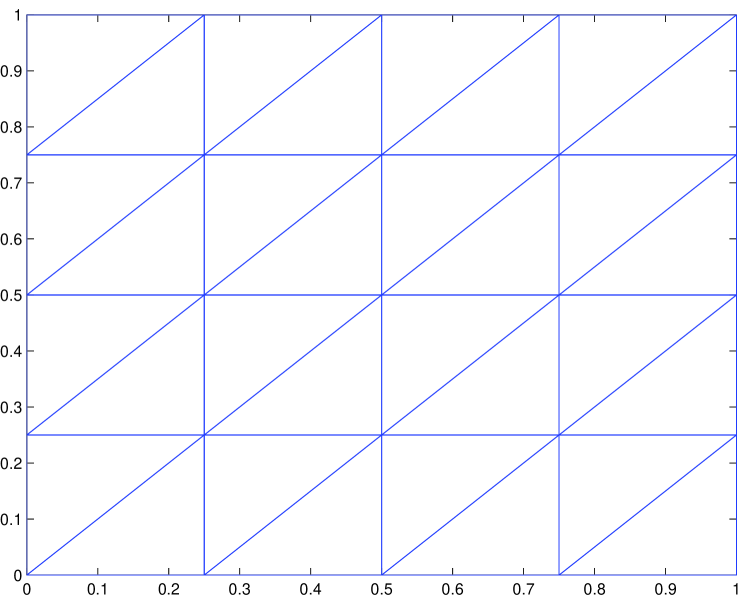
First, uniform mesh as in Fig 2 is considered. The fine meshes are of sizes () and the corresponding coarse meshes of size . Table 1 lists the numerical results for Algorithm 1. (i = 1) superconverges at rate of which consists with our theoretical analysis. However, (i = 1, 2, 3) ultraconverges at rate of which is better than the results predicted by Theorem 15. In particular, it verifies the statement in Remark 3.1. Since and are multiples eigenvalues, the error of eigenfunctions approximation are not available and it is represented by in Tables 1-7. One important thing we want to point out is that we observe numerically that obtained by Algorithm 1 approximates the exact eigenvalue from below; see column in Table 1. Similar phenomenon was observed in [15] where they use a local high-order interpolation recovery. We want to remark that lower bound of eigenvalue is very important in practice and there are many efforts are made to obtain eigenvalue approximation from below. The readers are referred to [3, 25, 44, 46] for other ways to approxiate eigenvalue from below. In Table 2, we report the numerical result of Algorithm 2. As expected, convergence of eigenvalue approximation and convergence of eigenfunction approximation are observed which validate our Theorem 21. The shift-inverse power method based two-grid scheme in [43, 21] is then considered, the result being displayed in Table 3. approximates (i = 1, 2, 3) at a rate and (i=1) converges at a rate of .
Comparing Tables 1 to 3, huge advantages of Algorithm 1 and 2 are demonstrated. For instance, on the fine grid with size and corresponding coarse grid with size , the approximate first eigenvalues produced by Algorithm 1 and 2 are exact up to digits while one can only trust the first five digits of the first eigenvalue generated by the two-grid scheme in [43, 21].
| i | H | h | ||||||
|---|---|---|---|---|---|---|---|---|
| 1 | 1/2 | 1/16 | 20.1083669 | 3.69e-01 | 20.2080796 | 4.69e-01 | 20.3504780 | 6.11e-01 |
| 1 | 1/4 | 1/256 | 19.7398503 | 6.41e-04 | 19.7398588 | 6.50e-04 | 19.7406011 | 1.39e-03 |
Then we consider the case for the first eigenvalue. We use the fine meshes of mesh size with and corresponding coarse meshes satisfying . The numerical results are showed in Table 4. We can see that the two proposed Algorithms give better approximate eigenvalues. Thus Algorithm 1 and 2 outperforms the two-grid scheme even in the case . One interesting thing that we want to mention is that approximates from above in this case, see column in Table 4.
| i | H | h | |||||
|---|---|---|---|---|---|---|---|
| 1 | 31 | 385 | 19.735647110619 | -3.56e-03 | 5.338236e-02 | ||
| 1 | 105 | 5761 | 19.739198229599 | -1.06e-05 | 2.15 | 2.835582e-03 | 1.08 |
| 1 | 385 | 90625 | 19.739208765246 | -3.69e-08 | 2.05 | 1.686396e-04 | 1.02 |
| 1 | 1473 | 1443841 | 19.739208802041 | -1.38e-10 | 2.02 | 1.049196e-05 | 1.00 |
| 2 | 31 | 385 | 49.307472112236 | -4.05e-02 | 0.00 | ———— | |
| 2 | 105 | 5761 | 49.347888708818 | -1.33e-04 | 2.11 | ———— | |
| 2 | 385 | 90625 | 49.348021524994 | -4.80e-07 | 2.04 | ———— | |
| 2 | 1473 | 1443841 | 49.348022003630 | -1.82e-09 | 2.01 | ———— | |
| 3 | 31 | 385 | 49.301142920140 | -4.69e-02 | 0.00 | ———— | |
| 3 | 105 | 5761 | 49.347856273486 | -1.66e-04 | 2.09 | ———— | |
| 3 | 385 | 90625 | 49.348021393237 | -6.12e-07 | 2.03 | ———— | |
| 3 | 1473 | 1443841 | 49.348022003123 | -2.32e-09 | 2.01 | ———— |
| i | H | h | |||||
|---|---|---|---|---|---|---|---|
| 1 | 31 | 385 | 19.739293668773 | 8.49e-05 | 9.258930e-03 | ||
| 1 | 105 | 5761 | 19.739209125443 | 3.23e-07 | 2.06 | 5.705799e-04 | 1.03 |
| 1 | 385 | 90625 | 19.739208803434 | 1.26e-09 | 2.01 | 3.555028e-05 | 1.01 |
| 1 | 1473 | 1443841 | 19.739208802184 | 5.33e-12 | 1.97 | 2.220103e-06 | 1.00 |
| 2 | 31 | 385 | 49.350648806465 | 2.63e-03 | 0.00 | ———— | |
| 2 | 105 | 5761 | 49.348029138391 | 7.13e-06 | 2.18 | ———— | |
| 2 | 385 | 90625 | 49.348022031328 | 2.59e-08 | 2.04 | ———— | |
| 2 | 1473 | 1443841 | 49.348022005547 | 1.00e-10 | 2.01 | ———— | |
| 3 | 31 | 385 | 49.351570779092 | 3.55e-03 | 0.00 | ———— | |
| 3 | 105 | 5761 | 49.348029733509 | 7.73e-06 | 2.27 | ———— | |
| 3 | 385 | 90625 | 49.348022033250 | 2.78e-08 | 2.04 | ———— | |
| 3 | 1473 | 1443841 | 49.348022005554 | 1.07e-10 | 2.01 | ———— |
| i | H | h | |||||
|---|---|---|---|---|---|---|---|
| 1 | 31 | 385 | 19.821235920927 | 8.20e-02 | 2.865766e-01 | ||
| 1 | 105 | 5761 | 19.744334806708 | 5.13e-03 | 1.02 | 7.159881e-02 | 0.51 |
| 1 | 385 | 90625 | 19.739529185236 | 3.20e-04 | 1.01 | 1.789929e-02 | 0.50 |
| 1 | 1473 | 1443841 | 19.739228826191 | 2.00e-05 | 1.00 | 4.474820e-03 | 0.50 |
| 2 | 31 | 385 | 49.828430094852 | 4.80e-01 | 0.00 | ———— | |
| 2 | 105 | 5761 | 49.377951127988 | 2.99e-02 | 1.03 | ———— | |
| 2 | 385 | 90625 | 49.349892261888 | 1.87e-03 | 1.01 | ———— | |
| 2 | 1473 | 1443841 | 49.348138895061 | 1.17e-04 | 1.00 | ———— | |
| 3 | 31 | 385 | 49.893495693695 | 5.45e-01 | 0.00 | ———— | |
| 3 | 105 | 5761 | 49.381970792689 | 3.39e-02 | 1.03 | ———— | |
| 3 | 385 | 90625 | 49.350143791388 | 2.12e-03 | 1.01 | ———— | |
| 3 | 1473 | 1443841 | 49.348154618353 | 1.33e-04 | 1.00 | ———— |
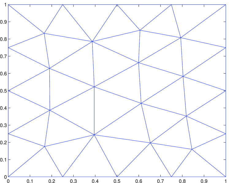
Now, we turn to unstructured meshes. First we generate a coarse mesh and repeat regular refinement on until to get the corresponding fine mesh . The first level coarse mesh is generated by EasyMesh [35] and the other three level coarse mesh are generated by regular refinement. The numerical results are provided in Tables 5 to 7. Note that and denote the number of vertices on coarse mesh and fine mesh , respectively. Concerning the convergence of eigenvalue, Algorithm 1 and 2 ultraconverge at rate while the two-grid scheme converges at rate . Note that in Tables 5.5–5.7, and . Therefore, convergent rates for and “double” the rates for and , respectively. As for eigenfunction, and are about while .
Example 2. In the previous example, the eigenfunctions are analytic. Here we consider Laplace eigenvalue value problem on the L-shaped domain . The first eigenfunction has a singularity at the origin. To capture this singularity, multilevel adaptive algorithms 3 and 4 are used with . Since the first exact eigenvalue is not available, we choose an approximation obtained by Betcke and Trefethen in [7], which is correct up to digits.
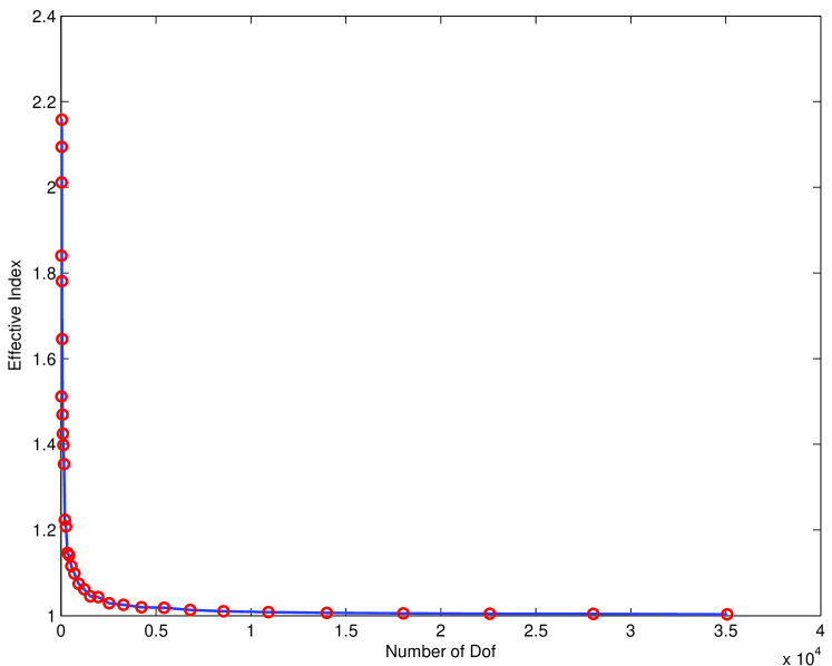
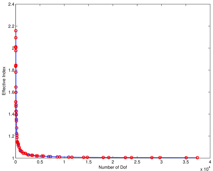
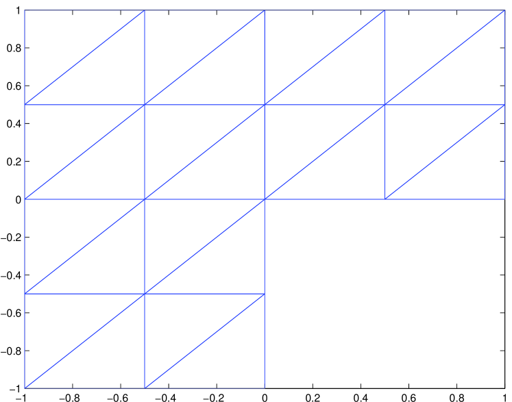
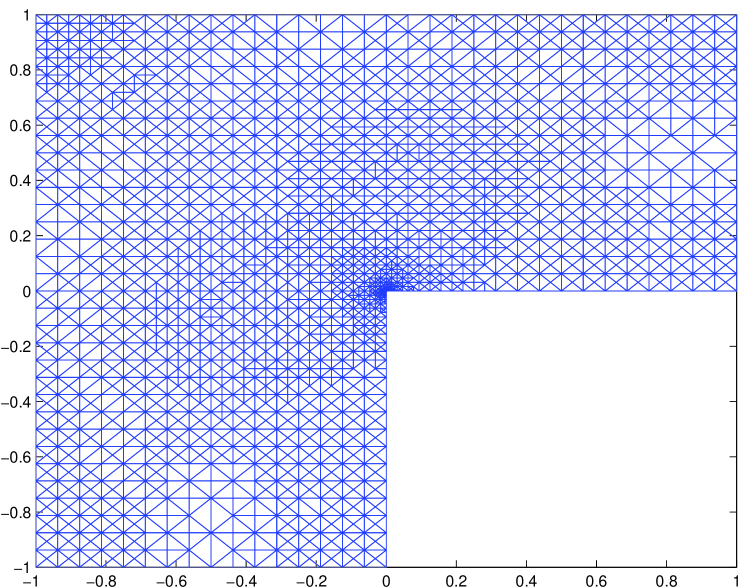
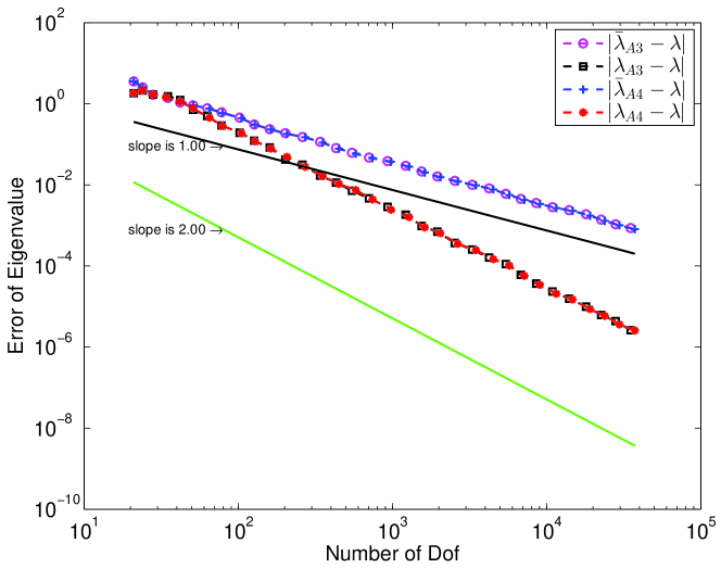
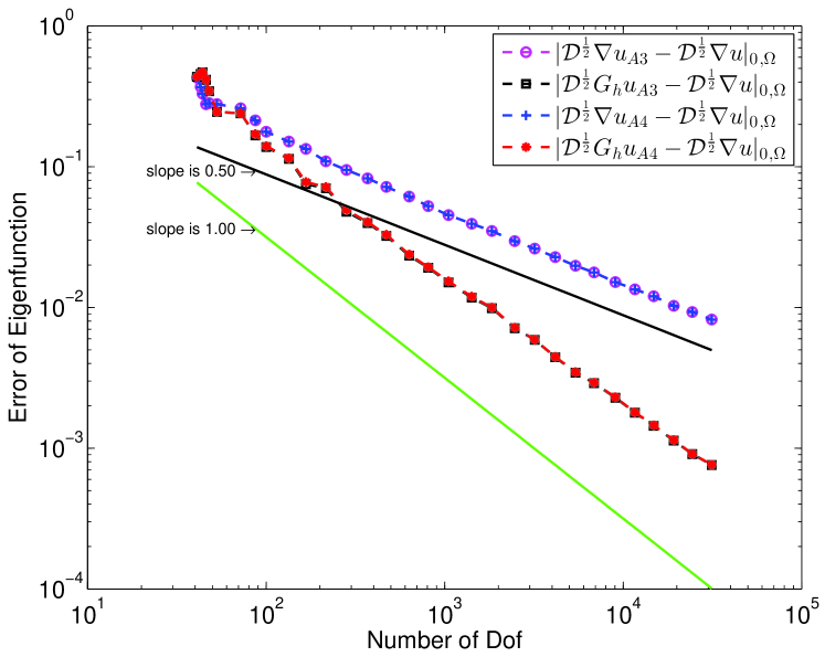
Fig 4 shows the initial uniform mesh while Fig 4 is the mesh after 18 adaptive iterations. Fig 5 reports numerical results of the first eigenvalue approximation. It indicates clearly and approximate at a rate of while and approximate at a rate of . The numerical results for Algorithms 3 and 4 are almost the same. Furthermore, we notice that and approximate the exact eigenvalue from below. It is well known that and are upper bounds for the exact eigenvalue. In actual computation, we use as stop criteria for adaptive Algorithm 3 where is the given tolerance. A similar procedure is applied to Algorithm 4.
In the context of adaptive finite element method for boundary value problems, the effectivity index is used to measure the quality of an error estimator [2, 4]. For eigenvalue problem, it is better to consider eigenvalue effectivity index insteading of traditional effectivity index in [2, 4]. In the article, we consider a similiar eigenvalue effective index as in [19]
| (29) |
where is either or and is either or . The effectivity index for the two proposed multilevel adaptive algorithms are reported in Figs 7 and 7. We see that converges to quickly after the first few iterations, which indicates that the posteriori error estimator (26) or (27) is asymptotically exact.
Example 3. Consider the following harmonic oscillator equation [18], which is a simple model in quantum mechanics,
| (30) |
where . The first eigenvalue of (30) is and the corresponding eigenfunction is with any nonzero constant .
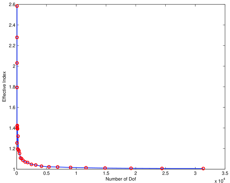
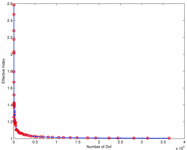
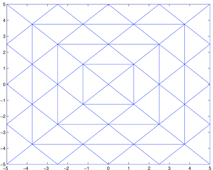
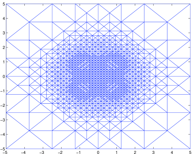
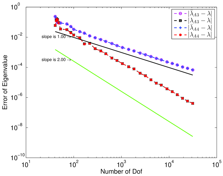
We solve this eigenvalue problem with and zero boundary condition as in [41]. The initial mesh is shown in Fig 9 and the adaptive mesh after 20 iterations is displayed in Fig 9. The parameter is chosen as . Numerical results are presented in Figs 11 and 11. For eigenvalue approximation, convergence rate is observed for while ultraconvergence rate is observed for . For eigenfunction approximation, and . The numerical result of Algorithm 4 is similar.
Figs 13 and 13 graph the eigenvalue effectivity index for the two proposed multilevel adaptive algorithms. It also indicates that the posteriori error estimator (26) or (27) is asymptotically exact for problem (30).
6 Conclusion
When eigenfunctions are relatively smooth, two-space methods (using higher-order elements in the second stage) is superior to two-grid methods (using the same element at finer grids in the second stage). They have the comparable accuracy. However, at the last stage, the degrees of freedom of the two-space method is much smaller than that of the two-grid method.
For linear element on structured meshes, using gradient recovery at the last stage achieves similar accuracy as the quadratic element on the same mesh. Therefore, with much reduced cost, the gradient recovery is comparable with the two-stage method on the same mesh.
Algorithms 3 and 4 use recovery type error estimators to adapt the mesh, and have two advantages comparing with the residual based adaptive algorithms. 1) Cost effective. In fact, the recovery based error estimator plays two roles: one is to measure the error, and another is to enhance the eigenvalue approximation. 2) Higher accuracy. Indeed, after recovery enhancement, the approximation error is further reduced.
References
- [1] A. B. Andreev, R. D. Lazarov, and M. R. Racheva, Postprocessing and higher order convergence of the mixed finite element approximations of biharmonic eigenvalue problems, J. Comput. Appl. Math., 182(2005), pp. 333–349.
- [2] M. Ainsworth and J. Oden, A posteriori error estimation in finite element analysis, Pure and Applied Mathematics, Wiley-Interscience , New York, 2000.
- [3] M. Armentano and R. Durn Asymptotic lower bounds for eigenvalues by nonconforming finite element methods, Electron. Trans. Numer. Anal.,17(2004), pp. 93–101.
- [4] I. Babuka and T. Strouboulis, The Finite Element Method and its Reliability, Oxford University Press, London, 2001.
- [5] I. Babuka and J. Osborn, Finite element-Galerkin approximation of the eigenvalues and eigenvectors of selfadjoint problems, Math. Comp., 52(1989), pp.275–297.
- [6] I. Babuka and J. Osborn, Eigenvalue problems, Handbook of numerical analysis, Vol. II, pp. 641–787, Handb. Numer. Anal., North-Holland, Amsterdan, 1991.
- [7] T. Betcke and L.N Trefethen, Reviving the method of particular solutions, SIAM Rev., 47(2005), pp.469–491.
- [8] S. Brenner and L. R. Scott, The mathematical theory of finite element methods, Third edition, Springer, New York, 2008.
- [9] F. Chatelin, Spectral approximation of linear operators, Academic Press, New York, 1983.
- [10] L. Chen, iFEM: An Integrated finite element package in MATLAB, Technical Report, University of California at Irvine, 2009.
- [11] C.-S. Chien and B.-W. Jeng, A two-grid discretization scheme for semilinear elliptic eigenvalue problems, SIAM J. Sci. Comput., 27(2006), 1287–1304.
- [12] P.G. Ciarlet, The Finite Element Method for Elliptic Problems, North-Holland, Amsterdam, 1978
- [13] W. Drfler, A convergent adaptive algorithm for Poisson’s equation, SIAM J. Numer. Anal., 33(1996), pp. 1106–1124.
- [14] R. Durn, G. Padra, and R. Rodrguez, A posteriori error estimates for the finite element approximation of eigenvalue problems, Math. Models Methods Appl. Sci., 13(2003), pp. 1219–1229.
- [15] J. Fang, X. Gao and A. Zhou, A finite element recovery approach approach to eigenvalue approximations with applications to electronic structure calculations, J. Sci. Comput., 55(2013), pp. 432–454.
- [16] X. Gao, F. Liu, and A. Zhou, Three-scale finite element eigenvalue discretizations, BIT, 48(2008), pp. 533–562.
- [17] D.S. Grebenkov and B.-T. Nguyen, Geometric structure of Laplacian eigenfunctions, SIAM Review, 55-4(2013), pp. 601–667.
- [18] W. Greiner, Quantum Mechanics: An Introduction, 3rd edition, Springer, Berlin, 1994.
- [19] S. Giani, L. Grubii and J. Ovall, Benchmark results for testing adaptive finite element eigenvalue procedures., Appl. Numer. Math., 62(2012), pp. 121–140.
- [20] R. H. W. Hoppe, H. Wu, and Z. Zhang, Adaptive finite element methods for the Laplace eigenvalue problem, J. Numer. Math., 18(2010), pp. 281–302.
- [21] X. Hu and X. Cheng, Acceleration of a two-grid method for eigenvalue problems, Math. Comp., 80 (2011), pp. 1287–1301.
- [22] K. Kolman, A two-level method for nonsymmetric eigenvalue problems, Acta Math. Appl. Sin. Engl. Ser., 21(2005), pp. 1–12.
- [23] H. Li and Y. Yang, The adaptive finite element method based on multi-scale discretizations for eigenvalue problems, Comput. Math. Appl., 65(2013), pp. 1086–1102.
- [24] Q. Lin and H. Xie, A Multi-level Correction Scheme for Eigenvalue Problems, arXiv:1107.0223 [math.NA].
- [25] Q. Lin, H. Xie and J. Xu, Lower bounds of the discretization error for piecewise polynomials, Math. Comp., 83(2014), pp. 1–13.
- [26] F. Liu, M. Stynes and A. Zhou, Postprocessed two-scale finite element discretizations, Part I., SIAM J. Numer. Anal., 49(2011), pp. 1947–1971.
- [27] H. Liu and N. Yan, Enhancing finite element approximation for eigenvalue problems by projection method, Comput. Methods Appl. Mech. Engrg, 233-236(2012), pp. 81–91.
- [28] M. G. Larson, A posteriori and a priori error analysis for finite element approximations of self-adjoint elliptic eigenvalue problems, SIAM J. Numer. Anal., 38(2000), pp. 608–625.
- [29] M. Mao, L. Shen, and A. Zhou, Adaptive finite element algorithms for eigenvalue problems based on local averaging type a posteriori error estimators, Adv. Comp. Math., 25(2006), pp. 135-160.
- [30] V. Mehrmann and A. Miedlar, Adaptive computation of smallest eigenvalues of self-adjoint elliptic partial differential equations, Numer. Linear Algebra Appl., 18(2011), pp. 387–409.
- [31] L. Meng and Z. Zhang, The ultraconvergence of eigenvalues for bi-quadrature finite elements, J. Comput. Math., 30 (2012), pp. 555-564.
- [32] A. Naga and Z. Zhang, A posteriori error estimates based on the polynomial preserving recovery, SIAM J. Numer. Anal., 42 (2004), pp. 1780–1800.
- [33] , The polynomial-preserving recovery for higher order finite element methods in 2D and 3D, Discrete Contin. Dyn. Syst. Ser. B 5 (2005), pp. 769–798.
- [34] A. Naga, Z. Zhang and A. Zhou, Enhancing eigenvalue approximatioin by gradient recovery, SIAM J. Sci. Comput., 28 (2006), pp. 1289-1300.
- [35] B. Niceno, EasyMesh Version 1.4: A Two-Dimensional Quality Mesh Generator, http://www-dinma.univ.trieste.it/nirftc/research/easymesh.
- [36] M. R. Racheva and A. B. Andreev, Superconvergence postprocessing for eigenvalues, Comput. Methods Appl. Math., 2(2002), pp. 171–185,
- [37] L. Shen and A. Zhou, A defect correction scheme for finite element eigenvalues with applications to quantum chemistry, SIAM J. Sci. Comput., 28(2006), pp. 321–338.
- [38] G. Strang, Gilbert and G. Fix, An analysis of the finite element method, Prentice-Hall Series in Automatic Computation. Prentice-Hall, Englewood Cliffs, 1973.
- [39] R. Verfrth, A review of a posteriori error estimation and adaptive mesh-refinement techniques, Wiley and Teubner, New York, 1996.
- [40] H. Wu and Z. Zhang, Enhancing eigenvalue approximation by gradient recovery on adaptive meshes, IMA J. Numer. Anal., 29 (2009), pp. 1008–1022.
- [41] H. Xie, A Multilevel Correction Type of Adaptive Finite Element Method for Eigenvalue Problems, arXiv:1201.2308v1 [math.NA].
- [42] J. Xu and A. Zhou, A two-grid discretization scheme for eigenvalue problems, Math. Comp., 70 (2001), no. 233, pp. 17–25.
- [43] Y. Yang and H. Bi, Two-grid finite element discretization schemes based on shifted-inverse power method for elliptic eigenvalue problems, SIAM J. Numer. Anal., 49 (2011), pp. 1602-1624.
- [44] Y. Yang, Z. Zhang and F. Lin, Eigenvalue approximation from below using non-conforming finite elements, Sci. China Math., 53(2010), pp. 137–150.
- [45] Z. Zhang and A. Naga, A new finite element gradient recovery method: superconvergence property, SIAM J. Sci. Comput., 26 (2005), pp. 1192–1213.
- [46] Z. Zhang, Y. Yang and Z. Chen, Eigenvalue approximation from below by Wilson’s element(Chinese), Math. Numer. Sin., 29(2007), pp. 319–321.
- [47] O. C. Zienkiewicz and J. Z. Zhu, The superconvergent patch recovery and a posteriori error estimates. I. The recovery technique, Internat. J. Numer. Methods Engrg., 33(1992), pp. 1331–1364.
