Stellar rotational periods in the planet hosting open cluster Praesepe

Abstract

By using the dense coverage of the extrasolar planet survey project HATNet, we Fourier analyze $381$ high-probability members of the nearby open cluster Praesepe (Beehive/M44/NGC 2632). In addition to the detection of $10$ variables (of $\delta$ Scuti and other types), we identify $180$ rotational variables (including the two known planet hosts). This sample increases the number of known rotational variables in this cluster for spectral classes earlier than M by more than a factor of three. These stars closely follow a color/magnitude – period relation from early F to late K stars. We approximate this relation by polynomials for an easier reference to the rotational characteristics in different colors. The total (peak-to-peak) amplitudes of the large majority ($94$%) of these variables span the range of $0.005$ to $0.04$ mag. The periods cover a range from $2.5$ to $15$ days. These data strongly confirm that Praesepe and the Hyades have the same gyrochronological ages. Regarding the two planet hosts, Pr0211 (the one with the shorter orbital period) has a rotational period that is $\sim 2$ days shorter than the one expected from the main rotational pattern in this cluster. This, together with other examples discussed in the paper, may hint that star-planet interaction via tidal dissipation can be significant in some cases in the rotational evolution of stars hosting Hot Jupiters.

1 Introduction

The well-known significance of open clusters in studying stellar evolution and various aspects of galactic structure and cosmic distance calibration has been highlighted recently by the analysis of the photometric databases collected by both target-oriented projects, such as the MONITOR project (e.g., Irwin et al., 2009) and by the ground- and space-based surveys of transiting extrasolar planets (TEPs). It is important to note that before these surveys and special projects, the data on rotational variables (i.e., on spotted stars with measurable photometric variability) were fairly scarce. For example, the first few variables of this type were discovered in the otherwise well-known nearby cluster Praesepe only in 2007 (Scholz & Eislöffel, 2007). The TEP surveys are very powerful means to discover variables, since they stare on the same large area of the sky for a period of three to six months (or longer) and gather good quality time series on $10^{4}$–$10^{5}$ stars in their large field of views. As a ‘by-product’ of these surveys, several open clusters were caught and analyzed in searching for TEPs and other variables, including spotted stars (Pepper et al. (2008), [Praesepe]; Collier et al. (2009), [Coma Berenices]; Hartman et al. (2010), [Pleiades]; Delorme et al. (2011), [Hyades, Praesepe]; Cargile et al. (2013) [Blanco 1]). These latter types of variables play a crucial role in studying stellar rotation and its dependence on cluster age and stellar type. For a very recent review of this field we refer to Bouvier et al. (2013).

Earlier studies on stellar rotation via photometric variability were limited due to the sporadic nature of the observational campaigns and their focusing mostly on individual targets. Furthermore, main sequence stellar rotational periods are in the range of few to $10$–$20$ days, which is not a comfortable range in following up low-amplitude variables with sparsely sampled ground-based observations. In addition, spot evolution and differential rotation lead to non-stationary frequency spectra, that may result in an inaccurate determination of the rotational periods, and in general, misinterpretation of the data. This is why previous works (before the era of TEP searches) were mostly limited to rotation effects producing signals above $\sim 0.01$ mag (e.g., Messina & Guinan, 2002). Even though most of the wide-field ground-based surveys are carried out from a single site, and thus have daily gaps in their observations, they are still capable of detecting rotation signals with amplitudes in the sub-mmag regime, thereby unveiling the rotation properties of stars with spot sizes similar to those on the Sun. This sensitivity results from the dense sampling, long time coverage, and relatively high photometric precision per observation achieved by these surveys (typical values are: cadences of a few minutes, $10^{3}$–$10^{4}$ total data points per star, and $0.01$–$0.02$ mag accuracy per data point). This dramatically increases the number of stars, from spectral types M to A, for which stellar rotational periods may be measured, and allows a deep analysis of angular momentum loss and stellar evolution.

From the point of view of extrasolar planets, open clusters are also important in addressing questions on the role of stellar environment in the early phases of planetary system evolution. Although considerable efforts have been made over the past to find planets in clusters using both spectroscopic (i.e., radial velocity) and photometric (i.e., transit) methods, these searches did not bear fruits until fairly recently. As of this paper, we know $11$ planets in six open clusters. We have three long period ($P>600$ days) radial velocity planets in the Hyades, NGC 2423 and NGC 4349 (Lovis & Mayor 2007; Sato et al. 2007). The other eight systems have shorter periods. There are two radial velocity planets in Praesepe ($P=4.43$ and $2.15$ days, Quinn et al. 2012), one in the Hyades ($P=6.09$ days, Quinn et al. 2014), three in M67 ($P=6.96$, $5.12$ and $121.71$ days, Brucalassi et al. 2014) and two TEPs from the Kepler satellite in NGC 6811 ($P=15.73$ and $17.82$ days, Meibom et al. 2013). Although this sample is still small, the number of planets hosted by cluster stars seems to be in agreement with those derived from field stars (this is true both for Hot Jupiters and for (sub)Neptunes – see Quinn et al. 2014 and Meibom et al. 2013, respectively).

Since the ages and the chemical compositions of the open clusters above are much more accurately known, than, in general, those of the field stars, with the five Hot Jupiters (HJs) residing in Praesepe, Hyades and M67, one can start addressing several questions (such as planet formation, migration and star-planet interaction) in a more efficient way. In particular, because of the usually well-defined rotational pattern of cluster stars, one may ask if tidal interaction between the planet and the star can lead to the spin-up of the host star (Brown et al. 2011; Penev et al. 2012; Zhang & Penev 2014). The difference between the rotational periods of single and planet host stars yields an important constraint on the tidal dissipation factors $Q_{\rm star}$ and $Q_{\rm planet}$. There are only bulk estimates on these parameters, although they are crucial in any tide-related problems (e.g., they scale the circularization and in-spiral times for close-in planets).

Using photometric time series observations from the HATNet project, here we derive rotational periods for $180$ K to F stars in Praesepe (M44/NGC 2632/Beehive). We use the tight period–color (also period–luminosity, or period–mass) relation spanned by these data to investigate the possibility of orbital momentum transfer in the two systems containing HJs. The results are compared with the Hyades, another planet hosting cluster, similar to Praesepe.

2 Frequency analysis of the cluster members

2.1 The HATnet data coverage

In selecting cluster members we rely on the membership analysis of Kraus & Hillenbrand (2007), based on various archival color, magnitude and proper motion data. In their Table 3 there are $1130$ stars listed as candidate cluster members, an overwhelming majority of which have large membership probabilities. Here we match all of them with the HATNet database and find that there are altogether $408$ objects that match within $0.22"$ of a HAT target (based on the 2MASS catalog). The remaining stars in the membership catalog yield much larger matching distances (greater than $9"$). This is because they have faint magnitudes and, as a result, they are absent from the HATNet database. Therefore, we have many inaccurate object identifications among the fainter stars with associated bad matching distances. This results in a poor sampling of the M dwarf regime, and, consequently, no coverage of the cooler M stars, where magnetic braking is not yet effective and the rotational periods have significant scatter due to the different initial conditions with which stars started their lives in the interstellar cloud. Although we have poor sampling in the M star regime, the HATNet survey is able to reach fast rotators at the blue end, which is also important, since this part of the diagram is still poorly known, largely due to the lower amplitudes of these variables. From the $408$ targets we omit $27$ which have a small number of data points and we end up with a sample of $381$ stars as the basic set for the frequency analysis..

Figure 1: Coverage of Praesepe by the HATNet fields. The $1130$ candidate members given by Kraus & Hillenbrand (2007) are shown as open circles.

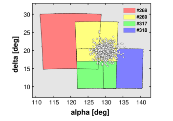
Praesepe has a very fortunate position in respect of the distribution of the HATNet fields. The cluster sits in the overlap area of four fields (see Fig. 1), yielding long-timebase coverage with high number of data points for most of the stars. Although there are four fields, their relative positions are such that cluster members may have only up to three-fold coverage. Further details of the field-wise data distribution are given in Table 1. The longest and most abundant coverage comes from the overlaps of fields #269, $317$ and $318$ with the total time span and datapoint number of 917 days and 14400, respectively. The integration time is $3$ min for all fields, except for #318, for which we used $5$ min integrations. With the read-outs and data storage, the sampling times are $\sim 20$% longer than these integration times. All observations were taken through the Sloan r filter.

Table 1: HATNet fields covering Praesepe.

Field	JDfirst	JDlast	T [days]	Ndp	N${}_{\rm clus}^{all}$	N${}_{\rm clus}^{act}$
268	55873	56070	197	7750	29	2
269	55674	55728	54	2750	403	374
317	55507	55672	165	8400	337	315
318	54811	54964	153	2900	278	241

Notes: JD_first, JD_last (minus $2400000$), T (total time span) and N_dp (number of data points) may change from object to object. The values listed are average values. N${}_{\rm clus}^{all}$: all overlaps with the cluster member list of Kraus & Hillenbrand (2007); N${}_{\rm clus}^{act}$: actual (N${}_{\rm dp}>1000$) overlaps with the list mentioned. Because the same object may appear in up to three fields, the total number of HATNet objects with cluster-membership and available light curve is only $381$.

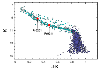
The distribution of the cluster member candidates of Kraus & Hillenbrand (2007) on the color-magnitude diagram (CMD) is shown in Fig. 2. The lighter/blue shade/color denotes the $408$ HATNet matches, including the two radial velocity (RV) planet hosts. This sample extends from early F to late K stars and follows a fairly well-defined isochrone corresponding to [Fe/H]$=0.11$ and age of $590$ Myr (Khalaj & Baumgardt 2013, see however Gaspar et al. 2009 for a possible higher age of $757$ Myr). A particular property of the CMD is the distinct high-luminosity branch between F- and early M-type stars. The common explanation of this branch is that these stars are either blended by some neighbors in the denser inner part of the cluster, or they are binaries with luminous secondary components (see, e.g., Khalaj & Baumgardt 2013, Wang et al. 2014). However, we note that an alternative explanation, involving an earlier mixing with another stellar population of different age may also be viable (Franciosini et al., 2003). It is also seen that the two planet hosts fit well to the densely-populated main sequence with no apparent second luminous components.

Figure 2: Color-magnitude diagram of Praesepe with the two planet host stars highlighted by larger filled circles. The $1130$ cluster candidates as given by Kraus & Hillenbrand (2007) are plotted in the 2MASS color system. The $408$ matching objects with the HATNet database are shown by light-shaded points.

2.2 Pre-analysis data conditioning

Since our time series preparation methods were developed in the context of transiting extrasolar planet search, we think it is useful to briefly describe the main aspects of our approach. For additional details on the two methods summarized below we refer to Kovács et al. (2005) and Bakos et al. (2010).

We use External Parameter Decorrelation (EPD) and Trend Filtering Algorithm (TFA) to clean up the data from systematics before the frequency analysis. These are crucial steps, since we usually deal with small-amplitude signals, that are either completely buried in the systematics or seriously crippled by them.

The idea of the EPD filtering is based on the observation that certain external parameters {$p_{\rm i}$} of the stellar image (such as PSF width, elongation, chip position, hour angle, color, etc.) correlate with $\Delta F$, which is the residual stellar flux after subtracting off the median of the signal. The functional form of $\Delta F(p_{1},p_{2},...)$ is determined numerically through a fit of {$p_{\rm i}$} to $\Delta F$ by using all individual flux measurements for each selected star. The correlation is determined for each star separately. Therefore, while the functional form of the correlation is the same, the regression coefficients will differ for each individual star. Once the correction function is found, it is employed on each star on each flux value individually by $F_{\rm corr}(t)=F_{\rm in}(t)-\Delta F(p_{1}(t),p_{2}(t),...)$, where $F_{\rm in}(t)$ is the incoming flux and {$p_{\rm i}(t)$} are the time-dependent external parameters. We note that although this step contains only the subtraction of a pre-determined function evaluated at the temporal values of the EPD parameters and stellar flux measurements, the regression is obtained by a fit to the target time series, and, as a result, the underlying signal might also be affected by this process. Our experience shows that this effect is usually small, and can be corrected at a later step with full time series model fitting (see Bakos et al. 2010).

TFA has a different philosophy in finding systematics in photometric time series. Akin in part to the traditional ensemble photometry, it is assumed that systematics exhibit themselves in many objects in a similar manner. In the case of standard ensemble photometry this behavior is simply utilized by calculating the average flux of a large number of neighboring stars and dividing the flux of the target by this average. However, in the case of TFA we assume that not all stars have the same systematics but for any given target we can find a time series {$Z(t_{\rm i})$} that is optimum in terms of systematics (i.e., it contains most of them, characteristic for the target signal). The optimization is achieved by using the time series of $m$ number of comparison stars (or templates) {$C_{\rm j}(t_{\rm i})$} and searching for the optimum filter {$U(t_{\rm i})$} in the form of the linear combination of these template time series: $U(t_{\rm i})=\sum_{\rm j=1}^{\rm m}a_{\rm j}C_{\rm j}(t_{\rm i})$. The regression coefficients {$a_{\rm j}$} can be found, e.g., by fitting {$U(t_{\rm i})$} to {$Z(t_{\rm i})$} by least squares. The filtered time series is obtained by subtracting {$U(t_{\rm i})$} from {$Z(t_{\rm i})$}. In this process we assume that the target time series is dominated by systematics - the non-reconstructive application of TFA. This assumption can be lifted once a signal is found, and a complete model is fitted that includes also the signal – the reconstructive application of TFA).

2.3 Frequency analysis

We employ the method of standard Discrete Fourier Transformation (DFT, Deeming 1975) to search for significant close-to-sinusoidal signals in the above dataset of $381$ light curves (LCs). The analysis is performed both on the basic product of the HATNet pipeline, comprising the time series after EPD and on the TFA-filtered time series of the EPD data. When analyzing the EPD data, we merge the LCs from the individual fields by shifting their averages to the same level. For the TFA-filtered data we perform non-reconstructive TFA filtering for each field separately, and then we merge the so-obtained LCs in the same way as we do for the EPD data. The analyses of the two types of datasets are complementary. The EPD data still contain various systematics, thereby weakening our ability to detect faint signals. On the other hand, application of TFA-filtering might lead to losing some of the variables due to over filtering, especially if they are on the longer period side and if there are other stars in the field with similar periods. Although our earlier works on different datasets (Szulágyi et al. 2009; Dékány & Kovács 2009) showed that the chance of this to happen is reasonably low, incorporating the original (EPD) data may further reduce the likelihood of this event. Furthermore, because several/many rotational variables in a cluster exhibit very similar periods, to minimize the effect of ‘squeezing’ the amplitudes when TFA is employed, we iteratively deselect suspected variables from the TFA templates.

In the variability search we test narrow-, medium- and high-frequency bands for the EPD and the TFA-filtered data. For the latter, we use $600$ templates selected as mentioned above. For the frequency bands we choose the ranges of $[0,0.5]$d^-1, $[0,10]$d^-1 and $[10,50]$d^-1. Both the frequency spectra and the folded LCs are examined. At the end of this process we conclude with $180$ rotational and $10$, mostly $\delta$ Scuti-type variables. The latter ones are summarized in the Appendix, whereas the rotational variables (including the selection procedure) are discussed in the subsequent sections.

3 Rotational variables

One of the distinct properties of main sequence cluster stars is that their rotational rates quickly (within a few hundred Myrs) settle down to a fairly tight sequence, usually parameterized by their mass, or by some other, observationally more easily accessible parameters, such as their colors (Barnes, 2003). Therefore, unlike in the case of rotating (i.e., spotted) variables in the field, they are much easier to recognize, especially if the cluster is rich, older than $\sim 100$ Myr and the underlying photometric data are accurate and extended enough to detect (quasi)periodic variation down to the mmag level.

Figure 3: Frequency versus approximate Sloan r(jhk) magnitudes for our Praesepe sample. All frequencies found as the highest peaks in the frequency spectra of the data and in their residuals after the first pre-whitening are plotted (i.e., two points for each star). The points are color/shade-coded from high signal-to-noise ratio (SNR$>8$, dark) to the low one (SNR$<5$, white). The analysis was made in the $[0,2]$ d^-1 frequency band. The derived rotation line (see text) is used to show the various frequency patterns due to aliases and confusion with harmonic components.

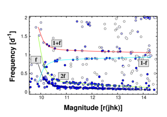
As an example of the striking appearance of rotational variables, in Fig. 3 we show all derived frequencies in the r(jhk)–frequency plane. The analysis covers the $[0,2]$d^-1 range and includes a single pre-whitening step for each star (i.e., we plot two frequency values for each of the $381$ stars: the peak frequencies obtained from the original and the pre-whitened data). The color coding for the signal-to-noise ratio (SNR) helps to recognize more easily the various ridges related to the main rotational sequence. The magnitudes in the Sloan r band are approximated by the following combination of the 2MASS colors (based on our linear regression to $410$ stars of Stetson 2000 with colors covering the range relevant for Praesepe) for Fig. 3, we decided to use exclusively these approximate Sloan r magnitudes, instead of mixing the two sets. In all other cases either the APASS or the 2MASS magnitudes are employed. We avoid using HATNet instrumental ‘r’ magnitudes, since the HATNet magnitudes are often unreliable, due to the limited spatial resolution of the images.

$${\rm r(jhk)}=0.6975+2.9782J-0.8809H-1.1230K\hskip 5.69054pt.$$ (1)

The rotational sequence (labelled by the letter ‘f’) shows up very clearly, as does the one related to the 1st harmonic (sequence ‘2f’). Other components, due to $1$ d^-1 aliasing (sequences ‘$1\pm f$’) show up too, albeit with a sparser population, indicating that in most cases aliasing is not an issue in the available dataset.

Figure 4: Dereddened Sloan r magnitudes versus period for our rotational variable star sample of $180$ stars in Praesepe (see Table 2). The continuous line is a 4th-order polynomial fit to the data (see Table 3). The two RV planet hosts of Quinn et al. (2012) are shown by the larger filled circles.

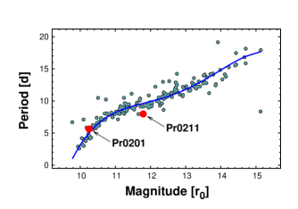
After the identification of the main rotational ridge, we go through the multistep variability check as described in Sect. 2.3 and construct the final rotational ridge by correcting the peak frequencies, if they belong to some of the secondary ridges mentioned above. Here we extend the correction due to harmonic components up to the 4th harmonic – because of the degeneracy between the observed and the rotational periods we may need to consider also these, more involved cases. In constructing the ridge, we iteratively develop the average ridge line, which is a 4th-order polynomial fit to the data. In deciding whether a frequency value should or should not be corrected for harmonics or aliases, we consider the difference between this frequency point and the one corresponding to the ridge value (at the given r magnitude). The consecutive steps in the frequency correction and polynomial fitting constitutes the iterative process.

Table 2: HATNet rotational variables in the Praesepe.

HAT ID/type	2MASS ID	$\nu$	1/T	B	V	r	K	J$-$H	J$-$K	A	SNR
		[d-1]	[d-1]	[mag]	[mag]	[mag]	[mag]	[mag]	[mag]	[mag]
HAT-269-0000500 b	08401762+194715	0.149427	0.0011	10.551	9.941	9.837	8.583	0.267	0.303	0.0044	10.5
HAT-269-0000588 b	08402231+200624	0.386161	0.0011	10.554	10.071	10.036	8.852	0.213	0.285	0.0036	7.6
HAT-269-0000592 b	08411002+193032	0.345078	0.0011	10.613	10.080	9.999	8.908	0.243	0.269	0.0045	9.4
HAT-269-0000667 b	08395234+191845	0.309961	0.0011	10.742	10.217	10.119	9.008	0.192	0.275	0.0042	8.3
HAT-269-0000673 b	08400062+194823	0.333975	0.0011	10.824	10.271	10.161	9.079	0.184	0.251	0.0072	6.5
HAT-269-0000610 d	08393042+200408	0.140742	0.0011	10.892	10.260	10.155	8.807	0.301	0.333	0.0054	5.9
HAT-269-0000701 d	08405252+192859	0.248768	0.0011	10.839	10.267	10.173	9.049	0.183	0.288	0.0047	5.7
HAT-317-0000737 b	08413154+183002	0.240999	0.0011	10.886	10.384	10.246	9.105	0.221	0.259	0.0075	12.8
HAT-317-0000748 c	08391096+181033	0.238181	0.0011	10.748	10.218	10.107	8.994	0.237	0.313	0.0031	6.3
HAT-270-0000544 c	08450422+202127	0.267231	0.0045	10.865	10.296	10.216	9.130	0.218	0.259	0.0060	6.8
HAT-269-0000768 b	08382429+200621	0.232577	0.0011	11.085	10.521	10.373	9.182	0.221	0.281	0.0161	14.7
HAT-318-0000612 c	08480173+184037	0.170922$\times 2$	0.0011	11.043	10.440	10.241	8.806	0.321	0.422	0.0101	9.3
HAT-269-0000761 c	08392498+192733	0.241306	0.0011	11.066	10.461	10.339	8.997	0.269	0.360	0.0073	8.0
HAT-269-0000805 c	08414382+201336	0.177573	0.0011	10.988	10.431	10.313	9.142	0.236	0.321	0.0066	8.2
HAT-318-0000683 d	08471411+162347	0.174265	0.0012	11.200	10.608	10.506	9.294	0.222	0.267	0.0155	12.8
HAT-270-0000640 b	08452794+213912	0.207376	0.0185	11.046	10.435	10.294	9.257	0.227	0.294	0.0082	5.0
HAT-269-0000861 b	08394575+192201	0.164439	0.0011	11.257	10.640	10.497	9.259	0.208	0.306	0.0089	8.9
HAT-269-0000834 b	08391217+190656	0.179223	0.0011	11.129	10.568	10.424	9.258	0.242	0.297	0.0040	6.6
HAT-270-0000678 b	08464732+193841	0.162909	0.0011	11.303	10.701	10.566	9.342	0.199	0.279	0.0070	9.2
HAT-269-0000794 b	08443703+194239	0.220523	0.0011	11.037	10.477	10.321	9.054	0.322	0.366	0.0081	9.8
HAT-269-0000877 d	08374660+192618	0.168159	0.0011	11.243	10.635	10.521	9.276	0.261	0.315	0.0095	7.1
HAT-269-0000850 b	08404189+191325	0.160327$\times 2$	0.0011	11.205	10.567	10.419	9.063	0.311	0.396	0.0173	3.8
HAT-269-0000905 b	08402271+192753	0.153421	0.0011	11.303	10.673	10.533	9.336	0.239	0.304	0.0096	12.8
HAT-269-0000871 d	08424525+185136	0.095443	0.0011	11.449	10.766	10.569	9.168	0.299	0.362	0.0047	11.7
HAT-269-0000913 d	08432019+194608	0.161667	0.0011	11.415	10.756	10.602	9.359	0.243	0.300	0.0103	10.9
HAT-269-0000885 b	08410961+195118	0.165487$\times 2$	0.0011	11.361	10.631	10.440	8.939	0.342	0.467	0.0114	15.6
HAT-317-0000999 b	08373307+183915	0.135465	0.0011	11.249	10.668	10.531	9.283	0.274	0.338	0.0069	12.0
HAT-269-0000946 d	08412584+195636	0.151615	0.0011	11.342	10.687	10.546	9.329	0.263	0.330	0.0087	9.9
HAT-269-0000936 b	08393553+185236	0.151867	0.0011	11.282	10.695	10.550	9.329	0.276	0.328	0.0176	14.4
HAT-270-0000714 c	08451310+194112	0.136573	0.0011	11.602	10.848	10.655	9.158	0.294	0.403	0.0067	8.7
HAT-317-0001078 b	08362782+175453	0.138810	0.0045	11.374	10.810	10.659	9.405	0.235	0.315	0.0083	5.8
HAT-317-0001111 b	08355455+180857	0.142247	0.0045	11.427	10.854	10.705	9.445	0.239	0.312	0.0059	9.0
HAT-269-0000993 d	08403992+194009	0.140088	0.0011	11.580	10.859	10.656	9.189	0.299	0.421	0.0113	13.5
HAT-269-0001025 b	08305546+193319	0.148258	0.0045	11.384	10.736	10.603	9.369	0.262	0.356	0.0119	11.2
HAT-269-0001089 c	08412869+194448	0.141959	0.0011	11.605	10.933	10.765	9.469	0.263	0.343	0.0057	10.9
HAT-269-0001128 d	08415587+194122	0.124125	0.0011	11.718	11.006	10.830	9.544	0.242	0.325	0.0127	13.2
HAT-269-0001075 d	08404798+193932	0.138748	0.0011	11.757	10.991	10.782	9.254	0.353	0.439	0.0093	13.9
HAT-269-0001149 d	08404832+195518	0.126479	0.0011	11.707	11.012	10.840	9.507	0.276	0.357	0.0155	11.9
HAT-269-0001058 d	08381427+192155	0.142596	0.0011	11.605	10.897	10.685	9.188	0.375	0.464	0.0097	10.8
HAT-269-0001147 b	08423225+192346	0.097807	0.0011	11.656	10.954	10.793	9.458	0.300	0.378	0.0069	9.8
HAT-269-0001124 d	08400635+191826	0.124386	0.0011	11.761	10.980	10.757	9.228	0.380	0.473	0.0067	11.3
HAT-269-0001249 d	08345963+210549	0.122355	0.0185	11.874	11.114	10.950	9.684	0.251	0.328	0.0156	8.3
HAT-269-0001268 d	08402743+191640	0.131965	0.0011	11.822	11.148	10.971	9.655	0.314	0.357	0.0129	14.0
HAT-269-0001333 c	08415437+191526	0.120981$\times 2$	0.0011	12.104	11.354	11.156	9.643	0.294	0.383	0.0347	19.1
HAT-269-0001377 b	08391499+201238	0.119970	0.0011	11.946	11.278	11.082	9.649	0.272	0.393	0.0071	14.0
HAT-269-0001340 b	08415924+205507	0.121889	0.0185	11.958	11.259	11.076	9.705	0.303	0.362	0.0098	3.6
HAT-269-0001410 b	08375208+195913	0.125548	0.0011	11.952	11.242	11.051	9.689	0.288	0.390	0.0159	10.8
HAT-269-0001400 c	08371148+194813	0.124051	0.0011	12.008	11.286	11.093	9.686	0.295	0.389	0.0066	7.3
HAT-269-0001405 d	08404248+193357	0.119527	0.0011	12.063	11.331	11.142	9.706	0.307	0.385	0.0064	8.0
HAT-269-0001431 b	08381497+203404	0.114133	0.0185	12.100	11.400	11.186	9.717	0.302	0.389	0.0103	9.8
HAT-269-0001352 c	08374998+195328	0.140085	0.0011	12.265	11.403	11.134	9.326	0.401	0.535	0.0135	12.5
HAT-269-0001402 d	08364896+191526	0.134236	0.0045	11.945	11.212	10.986	9.687	0.336	0.396	0.0109	7.9
HAT-269-0001517 d	08372222+201037	0.125524	0.0011	12.077	11.378	11.186	9.803	0.289	0.384	0.0085	11.1
HAT-269-0001467 d	08371829+194156	0.110117	0.0011	12.181	11.424	11.223	9.802	0.326	0.373	0.0039	7.9
HAT-318-0001287 c	08482783+182043	0.108759	0.0011	12.111	11.411	11.208	9.772	0.348	0.392	0.0061	8.0
HAT-269-0001515 d	08404761+185411	0.109594	0.0011	12.159	11.426	11.221	9.686	0.348	0.440	0.0059	8.2
HAT-269-0001544 b	08430055+202016	0.115043	0.0045	12.147	11.384	11.189	9.774	0.332	0.411	0.0052	9.1
HAT-269-0001510 d	08361639+193231	0.120615	0.0045	12.458	11.573	11.272	9.520	0.390	0.511	0.0123	7.9
HAT-269-0001490 b	08392858+192825	0.095355	0.0011	12.519	11.606	11.305	9.533	0.409	0.502	0.0062	11.6
HAT-269-0001570 b	08411031+194907	0.111032	0.0011	12.268	11.495	11.292	9.753	0.358	0.430	0.0096	9.4

Table 2: HATNet rotational variables in the Praesepe. – Continued

HAT ID/type	2MASS ID	$\nu$	1/T	B	V	r	K	J$-$H	J$-$K	A	SNR
		[d-1]	[d-1]	[mag]	[mag]	[mag]	[mag]	[mag]	[mag]	[mag]
HAT-317-0001886 a	08403360+184028	0.105660	0.0011	12.335	11.596	11.368	9.832	0.306	0.417	0.0054	12.9
HAT-269-0001637 c	08403169+195101	0.118601	0.0011	12.402	11.609	11.384	9.911	0.309	0.383	0.0035	9.5
HAT-317-0001780 d	08402440+182713	0.103601	0.0011	12.368	11.584	11.328	9.599	0.406	0.503	0.0090	9.8
HAT-269-0001650 d	08403184+201206	0.113741	0.0011	12.201	11.472	11.265	9.831	0.356	0.428	0.0055	8.6
HAT-269-0001741 d	08364572+200726	0.110516	0.0045	12.380	11.613	11.389	9.938	0.305	0.402	0.0139	8.8
HAT-269-0001710 d	08424250+190558	0.113111	0.0011	12.359	11.596	11.376	9.881	0.324	0.421	0.0159	14.2
HAT-269-0001674 d	08372755+193703	0.114988	0.0011	12.416	11.616	11.385	9.806	0.361	0.446	0.0140	14.5
HAT-269-0001632 d	08402863+201844	0.125217	0.0011	12.432	11.604	11.315	9.462	0.457	0.586	0.0071	8.1
HAT-269-0001790 d	08380808+202622	0.111455	0.0185	12.432	11.684	11.441	9.932	0.346	0.426	0.0154	5.3
HAT-269-0001789 d	08403623+213342	0.105293	0.0185	12.423	11.629	11.402	9.974	0.365	0.412	0.0077	7.7
HAT-269-0001917 c	08413384+195808	0.105716	0.0011	12.503	11.678	11.451	9.928	0.309	0.464	0.0039	6.9
HAT-269-0001771 a	08395983+193400	0.089919	0.0011	12.880	11.886	11.523	9.484	0.476	0.622	0.0120	14.8
HAT-269-0001893 d	08431076+193134	0.112537	0.0011	12.583	11.769	11.551	10.007	0.365	0.432	0.0141	13.7
HAT-269-0001932 b	08375703+191410	0.115590	0.0011	12.632	11.829	11.597	10.038	0.350	0.432	0.0108	12.4
HAT-269-0001910 d	08431784+203037	0.112342	0.0185	12.610	11.785	11.544	9.776	0.427	0.542	0.0245	4.7
HAT-269-0002062 d	08400968+193717	0.125705	0.0011	12.808	11.973	11.717	10.133	0.316	0.423	0.0141	9.8
HAT-269-0001961 b	08392155+204529	0.108068	0.0185	12.702	11.902	11.645	10.026	0.381	0.450	0.0132	6.2
HAT-317-0002172 b	08405967+182204	0.107968	0.0011	12.906	11.997	11.646	9.683	0.481	0.578	0.0049	8.0
HAT-270-0001619 d	08490670+194111	0.102851	0.0011	12.730	11.907	11.673	10.068	0.360	0.465	0.0079	9.5
HAT-269-0002072 b	08351780+193810	0.111128	0.0045	12.631	11.822	11.595	10.012	0.380	0.485	0.0071	7.6
HAT-269-0002135 b	08400416+194703	0.096288	0.0011	12.899	12.030	11.768	10.004	0.384	0.503	0.0076	10.8
HAT-269-0002031 d	08424372+193723	0.099158	0.0011	13.114	12.109	11.754	9.800	0.456	0.571	0.0059	8.2
HAT-269-0002148 d	08380758+195916	0.109603	0.0011	12.969	12.061	11.780	9.898	0.448	0.559	0.0157	12.6
HAT-269-0002273 d	08374739+190624	0.107563	0.0011	13.172	12.273	11.960	10.202	0.414	0.464	0.0155	12.4
HAT-269-0002449 d	08390228+191934	0.102145	0.0011	13.306	12.366	12.043	10.259	0.358	0.471	0.0113	9.5
HAT-269-0002316 d	08421149+191637	0.125418	0.0011	13.060	12.143	11.852	10.173	0.418	0.487	0.0170	13.3
HAT-269-0002419 d	08424021+190759	0.109495	0.0011	12.976	12.111	11.856	10.186	0.391	0.499	0.0092	11.6
HAT-269-0002450 b	08374640+193557	0.105249	0.0011	13.252	12.305	12.007	10.244	0.384	0.481	0.0153	13.0
HAT-269-0002492 b	08405669+194405	0.107877	0.0011	13.095	12.198	11.920	10.213	0.404	0.506	0.0132	10.8
HAT-269-0002593 d	08414368+195743	0.108949	0.0011	13.264	12.333	12.042	10.258	0.398	0.507	0.0114	14.1
HAT-269-0002482 b	08433880+221609	0.111669	0.0185	13.222	12.323	12.012	10.251	0.442	0.494	0.0112	4.4
HAT-269-0002573 d	08362269+191129	0.101991	0.0045	13.351	12.418	12.092	10.257	0.417	0.506	0.0212	11.9
HAT-317-0002919 b	08441706+184411	0.092146	0.0011	13.165	12.310	12.013	10.262	0.416	0.504	0.0041	9.2
HAT-269-0002527 b	08403347+193800	0.105467	0.0011	13.094	12.198	11.902	10.169	0.444	0.537	0.0162	14.3
HAT-269-0002623 d	08433239+194437	0.103944	0.0011	13.246	12.309	12.021	10.218	0.435	0.537	0.0118	13.5
HAT-317-0002964 b	08393752+181013	0.108451	0.0011	13.128	12.269	11.978	10.237	0.442	0.526	0.0132	13.7
HAT-269-0002678 a	08384610+203436	0.109185	0.0185	13.282	12.407	12.090	10.313	0.426	0.512	0.0148	8.4
HAT-269-0002756 d	08392185+195140	0.081829	0.0011	13.487	12.517	12.200	10.369	0.424	0.505	0.0076	8.8
HAT-269-0002682 b	08400571+190130	0.102428$\times 2$	0.0011	13.720	12.706	12.314	10.009	0.509	0.649	0.0466	17.9
HAT-269-0002812 d	08410725+192648	0.104281	0.0011	13.370	12.416	12.104	10.288	0.445	0.553	0.0131	11.4
HAT-269-0002804 b	08393836+192627	0.094945	0.0011	13.627	12.648	12.294	10.286	0.453	0.553	0.0114	9.6
HAT-269-0002837 b	08413070+185218	0.104063$\times 4$	0.0011	13.649	12.727	12.388	10.154	0.463	0.615	0.0553	16.1
HAT-269-0002769 a	08401571+195454	0.100648	0.0011	13.722	12.677	12.287	10.013	0.527	0.667	0.0132	12.3
HAT-269-0003067 d	08435467+185336	0.095532	0.0011	13.600	12.671	12.329	10.412	0.437	0.549	0.0153	13.3
HAT-269-0087638 d	08361410+193717	0.100242	0.0045	13.507	12.561	12.241	10.363	0.464	0.568	0.0077	7.2
HAT-269-0003068 b	08362830+201342	0.099556$\times 2$	0.0045	13.521	12.564	12.240	10.441	0.460	0.541	0.0066	5.8
HAT-269-0002891 d	08401893+201130	0.077013	0.0011	14.104	12.912	12.417	10.038	0.562	0.691	0.0092	11.9
HAT-269-0003096 b	08365411+184524	0.107872	0.0045	13.626	12.688	12.332	10.469	0.461	0.534	0.0111	10.8
HAT-269-0003250 b	08394707+194939	0.095265	0.0011	13.724	12.724	12.368	10.435	0.449	0.571	0.0088	8.9
HAT-317-0003872 b	08373821+182857	0.088607	0.0011	14.147	13.082	12.665	10.427	0.419	0.590	0.0262	18.6
HAT-269-0003348 d	08322347+205944	0.089952	0.0185	13.872	12.861	12.490	10.470	0.450	0.573	0.0169	4.7
HAT-317-0003864 a	08364711+183446	0.096869	0.0045	13.689	12.769	12.442	10.586	0.439	0.528	0.0135	13.1
HAT-270-0002625 a	08501855+192542	0.116183	0.0011	13.680	12.745	12.434	10.526	0.432	0.563	0.0045	5.8
HAT-269-0003407 b	08340436+203430	0.093106	0.0185	13.843	12.769	12.405	10.442	0.470	0.596	0.0194	5.1
HAT-269-0003424 b	08280099+195417	0.094660	0.0045	13.731	12.734	12.423	10.490	0.470	0.580	0.0053	6.6
HAT-269-0003584 d	08354516+193826	0.091304	0.0045	13.955	12.925	12.559	10.539	0.443	0.580	0.0116	6.8
HAT-269-0003387 d	08444870+201725	0.088264	0.0011	13.912	12.834	12.438	10.508	0.502	0.572	0.0135	11.2
HAT-269-0003664 d	08325223+195835	0.089051	0.0045	14.138	13.050	12.645	10.560	0.462	0.585	0.0206	10.4
HAT-269-0003588 d	08395998+193440	0.094691	0.0011	13.861	12.855	12.495	10.552	0.484	0.582	0.0198	13.4
HAT-270-0002790 b	08465012+210112	0.076449	0.0189	14.128	13.013	12.593	10.544	0.475	0.597	0.0098	7.4

Table 2: HATNet rotational variables in the Praesepe. – Continued

HAT ID/type	2MASS ID	$\nu$	1/T	B	V	r	K	J$-$H	J$-$K	A	SNR
		[d-1]	[d-1]	[mag]	[mag]	[mag]	[mag]	[mag]	[mag]	[mag]
HAT-269-0003629 b	08402624+191309	0.092922	0.0011	13.899	12.875	12.481	10.461	0.505	0.627	0.0102	12.0
HAT-317-0004241 d	08404439+183923	0.093539	0.0011	13.917	12.933	12.537	10.500	0.476	0.626	0.0187	14.5
HAT-317-0004286 b	08442031+180259	0.091827	0.0011	13.923	12.960	12.578	10.490	0.495	0.638	0.0070	8.4
HAT-269-0003847 a	08412258+185602	0.093008	0.0011	13.970	12.957	12.554	10.536	0.484	0.626	0.0273	19.9
HAT-269-0003924 d	08413902+191556	0.094158	0.0011	14.177	13.089	12.670	10.574	0.531	0.631	0.0092	11.2
HAT-269-0003973 b	08355988+193132	0.077594	0.0045	14.368	13.229	12.777	10.569	0.539	0.641	0.0079	9.1
HAT-269-0004092 a	08415884+200627	0.087139	0.0011	14.279	13.160	12.746	10.599	0.526	0.644	0.0141	11.1
HAT-318-0003767 d	08463355+181409	0.086355	0.0011	14.282	13.205	12.770	10.597	0.528	0.653	0.0195	13.3
HAT-269-0004164 d	08401345+194643	0.084119	0.0011	14.318	13.200	12.758	10.640	0.543	0.642	0.0138	13.3
HAT-269-0004180 d	08323341+200448	0.082029	0.0045	14.330	13.208	12.787	10.627	0.548	0.650	0.0164	11.9
HAT-269-0004361 b	08340356+194742	0.090750	0.0045	14.511	13.362	12.893	10.678	0.505	0.647	0.0098	10.0
HAT-269-0004323 d	08435672+194332	0.086016	0.0011	14.376	13.243	12.818	10.527	0.547	0.709	0.0169	12.7
HAT-270-0003419 a	08463304+185424	0.070295	0.0011	14.300	13.232	12.813	10.619	0.529	0.682	0.0173	17.8
HAT-269-0004069 a	08350805+195925	0.079749	0.0045	14.565	13.332	12.815	10.447	0.640	0.720	0.0095	9.6
HAT-269-0004532 b	08431522+200356	0.091513	0.0011	14.614	13.447	12.983	10.683	0.560	0.676	0.0163	16.0
HAT-317-0005295 a	08405865+184030	0.085103	0.0011	14.936	13.723	13.196	10.488	0.568	0.765	0.0152	12.1
HAT-269-0004773 a	08414818+192731	0.086184	0.0011	14.852	13.644	13.151	10.732	0.532	0.679	0.0170	15.0
HAT-269-0004680 b	08434356+190433	0.093232	0.0011	14.488	13.416	12.976	10.787	0.552	0.649	0.0062	8.0
HAT-269-0004793 d	08422008+190905	0.083953	0.0011	14.673	13.486	13.014	10.696	0.546	0.698	0.0072	8.0
HAT-317-0005320 d	08400984+180550	0.082000	0.0011	14.578	13.457	12.983	10.679	0.580	0.693	0.0101	11.0
HAT-269-0004728 d	08373624+191554	0.083522	0.0011	14.626	13.481	13.005	10.757	0.566	0.669	0.0157	11.5
HAT-269-0004769 a	08383723+190116	0.077810	0.0011	15.001	13.775	13.244	10.613	0.592	0.736	0.0107	10.7
HAT-269-0004494 b	08364957+193323	0.081739	0.0046	15.403	14.013	13.370	10.285	0.686	0.851	0.0191	13.5
HAT-269-0004958 a	08411992+193804	0.081357	0.0011	14.751	13.555	13.080	10.762	0.559	0.693	0.0109	10.4
HAT-269-0004816 b	08404426+202818	0.078254$\times 3$	0.0192	15.672	14.254	13.650	10.402	0.663	0.838	0.0692	6.1
HAT-269-0004795 b	08411319+193234	0.078417$\times 4$	0.0011	15.670	14.189	13.565	10.347	0.703	0.864	0.0370	16.8
HAT-317-0005953 d	08344714+180116	0.086052	0.0045	14.829	13.678	13.188	10.830	0.571	0.697	0.0165	11.8
HAT-269-0005580 b	08372638+192912	0.081849	0.0011	15.111	13.831	13.303	10.826	0.531	0.730	0.0135	10.8
HAT-269-0005408 d	08390411+193121	0.080736$\times 2$	0.0011	14.995	13.772	13.267	10.857	0.575	0.705	0.0088	5.9
HAT-269-0005362 a	08385722+201053	0.083890	0.0011	15.184	13.924	13.361	10.716	0.619	0.764	0.0204	13.6
HAT-269-0005801 a	08385833+193649	0.073795	0.0011	14.899	13.771	13.296	11.037	0.537	0.665	0.0125	11.9
HAT-269-0005589 d	08331762+192550	0.079399	0.0045	15.078	13.827	13.305	10.859	0.597	0.728	0.0178	10.2
HAT-317-0006380 d	08433105+183254	0.077285	0.0011	15.209	13.980	13.431	10.741	0.617	0.783	0.0076	8.1
HAT-269-0006020 d	08423700+200831	0.081840	0.0011	15.201	13.961	13.410	10.871	0.598	0.763	0.0261	14.1
HAT-269-0006002 d	08382963+195145	0.081521	0.0011	15.308	14.018	13.469	10.931	0.607	0.739	0.0200	15.7
HAT-317-0006654 d	08365374+182945	0.076722	0.0046	15.218	13.985	13.437	10.947	0.622	0.725	0.0172	9.4
HAT-269-0006168 d	08442652+194735	0.071629	0.0011	15.466	14.125	13.574	10.908	0.628	0.767	0.0182	9.9
HAT-317-0006713 d	08443613+183557	0.079219	0.0011	15.905	14.518	13.921	10.655	0.699	0.860	0.0236	9.8
HAT-269-0006357 b	08414934+191147	0.070891	0.0011	15.864	14.466	13.846	10.834	0.636	0.815	0.0154	8.3
HAT-269-0006450 b	08421664+200532	0.070833	0.0011	15.498	14.187	13.605	10.989	0.607	0.757	0.0183	9.4
HAT-269-0006795 b	08441324+184911	0.077282	0.0011	15.431	14.181	13.612	10.941	0.616	0.806	0.0213	15.1
HAT-269-0006689 d	08424596+211616	0.070576$\times 4$	0.0192	15.650	14.326	13.765	10.919	0.637	0.811	0.0311	5.2
HAT-269-0006856 b	08400070+191834	0.070008	0.0011	15.805	14.427	13.829	10.918	0.648	0.826	0.0212	11.2
HAT-269-0007142 b	08313281+210128	0.052230$\times 2$	0.0192	15.881	14.573	13.979	11.118	0.636	0.767	0.0658	7.8
HAT-269-0007074 b	08391580+200414	0.065576$\times 2$	0.0048	16.432	14.946	14.292	10.867	0.686	0.871	0.0369	8.8
HAT-269-0007168 a	08411541+200216	0.073167	0.0011	15.563	14.230	13.669	11.022	0.657	0.811	0.0248	12.2
HAT-269-0007109 b	08365680+190528	0.067361	0.0047	16.115	14.659	14.047	10.974	0.680	0.829	0.0222	9.7
HAT-269-0006935 b	08312987+202437	0.089114$\times 4$	0.0208	15.766	14.351	13.729	10.767	0.725	0.907	0.0459	5.3
HAT-317-0008551 d	08405531+183459	0.080526	0.0011	15.838	14.507	13.911	11.128	0.660	0.796	0.0165	10.8
HAT-270-0006183 b	08534667+191814	0.072508	0.0065	16.282	14.798	14.207	11.165	0.660	0.808	0.0278	6.3
HAT-269-0008437 b	08363642+191106	0.074895	0.0047	16.180	14.719	14.107	11.199	0.600	0.820	0.0254	9.6
HAT-269-0008217 a	08314045+194754	0.057273$\times 2$	0.0048	16.580	15.098	14.495	11.027	0.694	0.890	0.0615	9.4
HAT-269-0008376 d	08305102+192108	0.070732	0.0047	16.101	14.752	14.176	11.193	0.661	0.829	0.0194	9.2
HAT-317-0010700 a	08415228+180306	0.064425	0.0012	16.451	15.091	14.470	11.337	0.661	0.833	0.0236	10.3
HAT-269-0009602 a	08394103+195928	0.059496$\times 4$	0.0061	17.053	15.339	14.736	11.323	0.679	0.854	0.0611	7.2
HAT-318-0009219 a	08492676+183119	0.055142$\times 2$	0.0012	16.819	15.396	14.771	11.394	0.656	0.847	0.0742	11.2
HAT-317-0011466 a	08412417+181402	0.119670$\times 4$	0.0067	17.082	15.787	15.193	11.455	0.660	0.824	0.1061	7.1
HAT-269-0010318 b	08393645+192907	0.063811	0.0011	16.544	15.106	14.501	11.391	0.652	0.863	0.0239	8.9
HAT-318-0010036 a	08483271+165623	0.055839$\times 3$	0.0065	17.240	15.759	15.200	11.468	0.625	0.860	0.0726	8.0
HAT-317-0012279 b	08363256+162302	0.063021	0.0061	16.839	15.369	14.770	11.508	0.649	0.839	0.0388	6.3

Notes: Variable types based on the classification of their frequency spectra (see Sect. 3.3) are shown in the second column. Frequencies flagged by $\times n$ indicate that the value shown is $1/n$-th of the most dominant frequency of the DFT spectrum. As a proxy of the error of the frequencies, we list the inverse of the total time span (T). The B, V, Sloan r, K, J$-$H and J$-$K magnitudes are from the APASS and 2MASS databases, respectively. Amplitudes (A) are peak-to-peak values from the 4^th order Fourier fit to the data without TFA filtering and using the frequencies as given in this table. The signal-to-noise ratio (SNR) of the peak frequency is computed from the data without TFA filtering and refers to the $[0,0.5]$ d^-1 band.

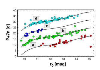
After multiple screenings of all the stars analyzed, we end up with $180$ rotational variables (see Table 2). The positions of these stars on the r[mag]–period plane are shown in Fig. 4. We see that indeed, the relation is fairly tight, although there are some $13$ outliers (arbitrarily defined as those with relative distances from the ridge greater than $20$ % – i.e., $|\nu/\nu_{\rm ridge}-1|>0.2$). Except perhaps for a few low-SNR variables, all are very secure detections. None of them have other frequencies in the $[0,50]$ d^-1 band (except for possible harmonic components). Some of them at the fainter (redder) end may well belong to the group of stars that have not yet converged to a tight rotational sequence. An additional source of ambiguity in this diagram is the reliability of the associated magnitude/color values. These might be strongly affected by blending in the more crowded region of the cluster. We also mention that except for two (HAT-269-0000761 and HAT-269-0000794) of the $24$ spectroscopic binaries common with the list of Mermilliod et al. (2009), all follow the overall r[mag]–period relation shown in Fig. 4.

It is important to note that we also detected the rotation of the two planet hosts. The ratios of the orbital to the rotational periods are non-commensurate in both systems. For Pr0201=HAT-269-0000805 $P_{\rm orb}/P_{\rm rot}=0.787$ whereas for Pr0211=HAT-269-0002316 this ratio is $0.270$. This further supports the planetary nature of these systems, since the periods of the radial velocity signals are not integer multiples/fractions of the rotational periods as one might expect if the radial velocity variations were caused by stellar activity.

In comparison with similar plots from other clusters, it is seen that we miss the faint end of the progression, where the lack of magnetic braking shows up as a suddenly increased scatter in the periods. Our survey (similarly to that of Delorme et al. 2011) is too shallow to cover this rather faint magnitude range. However, the PTF project covered just this range for this cluster, and, indeed, found $40$ variables with a wide period range of $0.5$ to $36$ days (Agüeros et al., 2011). Similarly, the deep survey by Scholz et al. (2011) resulted in the discovery of $26$ fast rotating ($P_{\rm rot}<2.5$ d) objects in the very low ($M<0.3M_{\odot}$) mass regime. The recent analysis by McQuillan, Aigrain & Mazeh (2013) confirms this wide period distribution also for the Kepler field M stars. Toward the blue end, on the other hand, due to the field overlaps, our survey is sensitive to periodic variations down to a few mmag. This leads to a good coverage of the progression in this regime, where the roughly linear color dependence becomes nonlinear and the rotational periods get rather short. For other clusters, a more detailed exploration of this regime is under way by the analysis of the data from the Kepler satellite (see Meibom et al. 2011 on NGC 6811 and Balona et al. 2013 on NGC 6866).

It is interesting to compare the list of the $52$ rotational variables published by Delorme et al. (2011) from the SuperWASP survey, covering basically the same color and magnitude range as HATNet. We find matching HATNet targets for all $52$ stars, $7$ of which are not included in the Kraus & Hillenbrand (2007) list of cluster members. Our data do not yield significant signals for $13$ stars. (Although some of them may be present in the original EPD data without TFA filtering, we do not consider them as valid detections until they are confirmed by the analysis made on the TFA-filtered data.) For the remaining $39$ mutual detections we have good agreement between the SuperWASP and HATNet frequencies (with relative frequency differences of $|\nu_{\rm HAT}/\nu_{\rm WASP}-1|$ within $10$% for the mutually detected $39$ stars and within $3$% for $75$% of these stars).

The two highlighted planet hosts (see the bigger filled circles) basically follow the overall rotational trend, but the fainter one seems to fall a bit on the short-period side. In Sect. 4 we further discuss the relation of these and other planet hosts to the overall rotational patterns in different clusters.

For an easier reference to the ridge values in the various colors, we fit $m$-th order polynomials to the respective color-period relations

$$P=\sum_{i=1}^{m+1}a_{i-1}x^{i-1}\hskip 5.69054pt,$$ (2)

where $x=k({\rm c}-<c>)$, $k=2/(\rm{cmax}-\rm{cmin})$, $<c>=(\rm{cmax}+\rm{cmin})/2$ and $\rm{cmin}$, $\rm{cmax}$, respectively, refer to the (min,max) values of the given dereddened color ‘$c$’ in the region we fit the periods. Dereddening is performed with $E(B-V)=0.027$ and standard relative reddening coefficients (e.g., Yuan et al. 2013). For V, B$-$V and Sloan r the order of the polynomial ($m$) is equal to $4$, whereas for the 2MASS colors we choose $m=3$, because of the lower stability of the fit for these colors at higher polynomial orders. In finding the best fit to the ridge, we employ sigma clipping at the level of $2.5\sigma$. The resulting coefficients are listed in Table 3.

Table 3: Polynomial fits to the ridge values.

color	$a_{0}$	$a_{1}$	$a_{2}$	$a_{3}$	$a_{4}$	cmin	cmax
V	$10.724$	$4.356$	$3.011$	$3.240$	$-3.942$	$9.941$	$15.787$
B-V	$11.528$	$4.934$	$1.277$	$1.446$	$-2.897$	$0.483$	$1.714$
r	$10.006$	$3.132$	$1.147$	$3.483$	$-2.233$	$9.906$	$14.218$
K	$9.579$	$4.633$	$-0.755$	$4.083$	$0.000$	$8.580$	$11.505$
J-H	$10.380$	$3.917$	$-0.240$	$2.096$	$0.000$	$0.180$	$0.722$
J-K	$10.447$	$2.975$	$0.675$	$4.020$	$0.000$	$0.247$	$0.903$

Notes: See Eq. (2) and the subsequent explanation for the use of the data in this table. By omitting outliers at the $3\sigma$ level, the above regressions fit the $180$ rotational variables with standard deviations of $0.7$, $0.9$, $0.7$, $1.0$, $1.2$ and $1.2$ days for V, B$-$V, r, K, J-H and J-K, respectively. The number of the corresponding outliers are $11$, $7$, $11$, $8$, $5$ and $3$.

3.1 Compatibility with the observed rotational velocities

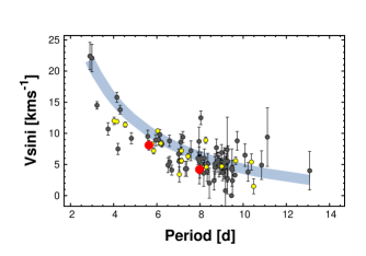
If spectroscopic $V_{\rm rot}\sin i$ values are available, it is customary to compare these values with the derived rotational periods. We use the data from the spectroscopic survey of open clusters by Mermilliod et al. (2009). By cross-correlating the data published for Praesepe with our rotational variable list, we find $88$ matches. These stars are plotted in Fig. 5. For the computation of the expected rotational rates we estimate the radii of the stars by using the Padova isochrones for the age of $590$ Myr with solar-scaled composition at $Z=0.02$. For the overall cluster reddening we set $E(B-V)=0.027$ mag and for the distance modulus we use $6.30$ mag. These values are taken from Fossati et al. (2008), Boesgaard & Roper (2013), Taylor (2006) and van Leeuwen (2009) and are in the overall ranges of the most frequently quoted parameters for this cluster.

Although the isochrone corresponding to the above parameters fits the ($J-K$, $K$) diagram quite well in the $J-K$ regime between $0.2$ and $0.8$, it fails to reproduce the break at $J-K\sim 0.85$. As discussed by Khalaj & Baumgardt (2013), other isochrones fit this particular part better but are less successful in reproducing the hotter part of the main sequence. Since we are focusing on stars between A and M spectral types, and our experiments with other isochrones led to similar results to those of the Padova isochrones, we decided to use these latter ones in the estimation of the stellar radii. We found that the computed stellar rotational velocities can be well fitted by the following simple formula

$$V_{\rm rot}=57.0P_{\rm rot}^{-(1.0+0.03(P_{\rm rot}-6.0))}\hskip 5.69054pt,$$ (3)

where $P_{\rm rot}$ is the measured rotational period (in [days]). The thickness of the line shown in Fig. 5 covers the range of scatter due to observational errors in the 2MASS colors. It is important to note that the above formula can be employed only on this cluster, since it depends on the age and chemical composition, specific to this cluster.

We think that the agreement between the observed and expected rotational velocities is reasonably good. For ideal (errorless) observed rotational velocities we should see the ‘theoretical’ equatorial velocities (thick gray line in Fig. 5) as the upper envelope of the observed values. We see that some stars are above this line. Several of them have reasonably large error bars to consider their outlier status insignificant, but some of them may pose some concern, such as HAT-269-0001124 at the period of $8.04$ d with small error and well-established period.

Figure 5: Photometric periods versus observed rotational velocities by Mermilliod et al. (2009) for the objects in common with our list of rotational variables (see Table 2). The RV planet hosts are shown by the bigger filled circles, the spectroscopic binaries from Mermilliod et al. (2009) by the ones with lighter shade. The thick continuous line is drawn by using Eq. (3). The line covers the stellar rotational velocities derived from the observed rotational periods and stellar radii given by model isochrones.

3.2 Color – amplitude dependence

It is important to investigate if the amplitude of the observed variability has any tendency of a correlated variation with some other properties of the star. Such a correlation might be expected from the underlying dependence of stellar activity on the same parameters (e.g., Mamajek & Hillenbrand 2008). Because the observed photometric amplitude is a multivariable function of the complicated physical processes (rotation, local and global magnetic field variations, convection, turbulence, etc.) involved in the spot generation and also of the specific geometric configuration, we expect rather fuzzy relations between the amplitudes and some other observable parameters. Indeed, results published so far show that the relation is fairly vague, especially if we are aimed at a more comprehensive analysis (see Saar et al. 2011 for a step in this direction).

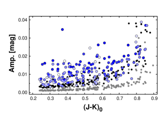
To add further piece of information to this issue, by using the data of Table 2, we show the variation of the peak-to-peak amplitudes as a function of $(J-K)_{0}$ in Fig. 6. The dependence is similar to most of the published results; redder (fainter, longer-period) stars tend to have larger amplitudes. We note that employing the Rossby number (the ratio of the rotation period to the convective turnover time – see Noyes et al. 1984), advocated by some studies (e.g., Hartman et al. 2009, Walkowicz & Basri 2013), yields also consonant result with similar scatter. Because of the data are more noisy and may contain less data points at the red (faint) end, we must address the question if the observed trend is the result of noise-limited sampling. By using the simple assumption of Gaussian white noise, the Fourier amplitudes follow a frequency-independent $\chi$ distributions, therefore we can compute the average expected Fourier amplitude as $<A_{\rm noise}>=\sqrt{\pi/N}\sigma$. Here $N$ is the number of data points and $\sigma$ is the (assumed to be) uniform point-by-point standard deviation of the data. We estimate the expected signal amplitudes at the detection level of $k\sigma$ as $k<A_{\rm noise}>$. It is seen that the higher significance lower limits (black dots) nicely follow the lower boundary of the amplitudes of the detected variables. The lower significance lower limits (gray dots) show the same trend but rendering the suspected trend significant. Considering that our assumption on the noise properties is a gross simplification of the real data setting with gaps, systematics and associated colored noise, we incline to conclude that most of the observed trend comes from the lower signal detection efficiency at the high-noise end. The similarity of the trend of the statistical limit to that of the lower boundary of the variables also supports this conjecture.

Figure 6: Variation of the peak-to-peak amplitudes (see Table 2) as a function of the 2MASS $(J-K)_{0}$ color (large shaded circles, with shading code from $SNR\leq 4$ [white] to $SNR\geq 14$ [deep blue/gray]). For reference, the $5$ and $15\sigma$ limits of signal detection (assuming white noise) are also shown on a star-by-star basis by gray and black filled circles, respectively. In order to scale the figure to the bulk of the sample, we left out a handful of stars with amplitudes larger than $0.04$ mag. The apparent trend in the amplitudes is most likely associated with the higher detection limit toward redder colors (i.e., fainter stars).

3.3 The four types of variability

One particular problem with the photometric identification of the rotating variables is that the corresponding time series are non-stationary due to the finite life time and migration of the spots to different latitudes, where differential rotation leads to a frequency drift in the observed signal. In spite of this, it is expected that some level of coherence prevails and leads to a broad, but still well-defined peak in the frequency spectrum.

Although the peak profiles can supply valuable information on spot life times and migration/differential rotation, the current data are still not suitable for this kind of deep analysis, due to the interfering noise and gaps in the sampling. Nevertheless, some basic properties are easy to recognize and one can classify the observed frequency spectra based on these simple characteristics. Although this classification is phenomenological in nature, it adds further solid information to the occurrence rates of the most common types of rotation-induced variability.

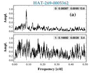
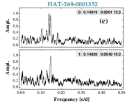
Upon examining the frequency spectra (with some representative examples shown in Fig. 7), we find that all $180$ stars classified as rotational variables fall in one of the following categories.

Figure 7: Examples for the four types of frequency spectra of the rotational variables as discussed in Sect. 3.3. In each sub-figure the upper and lower panels show, respectively, the frequency spectra of the data and the spectra obtained after the first pre-whitening (with the peak frequency shown on the upper panel). The insets display the pre-whitening order, the peak frequency, the amplitude and the SNR of the peak. The spectra are normalized to the highest peak in each panel.

1. These variables apparently have monoperiodic sinusoidal light variation (i.e., no residual power left near the main peak after pre-whitening). We have $23$ such cases in the present sample, which constitutes $13$% of the rotating variables.

2. There are $71$ variables (i.e., $39$% of the full sample) with a single but unstable sinusoidal component. Because of the frequency/amplitude drifts, these variables have inherently non-discrete Fourier spectra. Therefore, they show residual power close to the peak frequency even after several pre-whitening cycles (based on the piece by piece signal removal, assuming stationarity for each component).

3. In $13$ infrequent cases we can observe two peaks separated by a few times of the overall line width (i.e., by $\Delta\nu=1/220$d^-1, where the basic time span of $220$ days is determined by the compact/$\sim$continuous time base of two of our fields, #$269$ and $317$). The frequency distances are between $\sim 0.007$d^-1 and $\sim 0.020$d^-1 (with the exception of HAT-270-0000714, that has frequency components separated by $\sim 0.032$d^-1). The most common explanation of these separate components is that they are associated with the different latitudes of the stellar surface, that, due to differential rotation, carry the respective spots with different periods. We note that even the largest frequency separation is allowed by current models of differential rotation (e.g., Kitchatinov & Olemskoy 2012). These $13$ stars constitute $7$% of the full sample.

4. As already indicated in Fig. 3, most of the frequencies with sufficient significance that do not sit on the main rotational ridge in the color/magnitude – period plot belong to the first harmonic of the rotational frequency. The first harmonic may have larger or smaller amplitude than that of the rotational frequency. There are altogether $73$ stars (i.e., $41$% of the sample) that have residual power either at the corresponding 1st harmonic or at a sub-harmonic frequency. The effect of the harmonics may show up either as a non-sinusoidal distortion or as a double hump in the light curve, indicating more complicated spot distribution in the latter case.

It maybe useful to investigate how the above type of formal classification relates to other parameters, in particular to the magnitudes or colors. In Fig. 8 we plot the above classes separately in the $r_{0}$ – $P$ plane. Interestingly, not all types of variables are distributed evenly in this plane. Although the particular distributions are related to the types with relatively low number of members, we think that for type (c) (variables with two closely spaced frequencies) and maybe also for type (a) (those with constant amplitude sinusoidal variations) we may state that they are preferably found at high and low/mid luminosities, respectively. Although we cannot offer an explanation for this distribution pattern at this moment, it is important to note that for short rotation periods (i.e., higher luminosities) differential rotation results in a larger difference in the rotational periods between the pole and the equator (e.g., Kitchatinov & Olemskoy 2012). Therefore, for hotter (fater rotating) stars, frequency splitting due to differential rotation might be more easily observed and disentangled from line profile broadening due to the nonstationary nature of the spots. On the other hand, the observed frequency spacings do not increase with the luminosity as one might expected from the result of Kitchatinov & Olemskoy (2012).

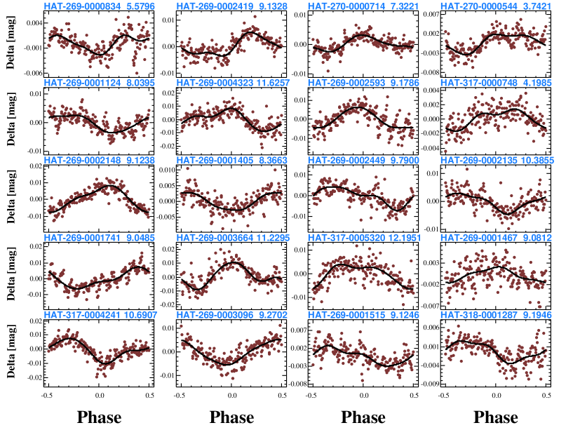
Finally, for a more direct inspection of the rotational variables, we display some mid-SNR LCs in Fig. 9. It is seen that non-sinusoidal variations are quite common and the LCs are diverse as expected from different geometrical and spot configurations.

Figure 8: Rotational variables plotted in the dereddened Sloan r magnitude – period plane and separated according to the classification presented in Sect. 3.3. For better visibility, the various classes are shifted by 7 days in the vertical directions (with type (a) left at the original periods).

Figure 9: Example of the mid-SNR light curves from the $180$ rotational variables. For better visibility, the light curves are binned in $200$ bins. The corresponding 3rd-order Fourier fits are shown by continuous lines. The folding period is equal to the rotational period (see Table 2) and shown (in [days]) in the upper right corner of each panel. For this plot we use the original (i.e., EPD, non-TFA-filtered) data. As a result, some of the light curves may contain substantial amount of systematics (e.g., HAT-269-0000834). Phase zero corresponds to HJD 2456000.0 .

4 Do close-in planets spin up their host stars?

For close-in planets it is an important question if tidal interaction has any influence on the dynamics of the system, including the rotation of the star. For individual systems in the field it is often difficult to study this question, since most of the parameters (e.g., age, rotational period) necessary to make any reasonably solid statement on this interaction, are among the least accurately determined quantities for single free-floating stars.

Figure 10: Period–(J$-$K)₀ plot for Praesepe (light filled circles, this paper) and for the Hyades (dark filled circles, Delorme et al. 2011). The RV planets (Quinn et al. 2012, 2014) are shown by the larger filled circles; darker shade for Praesepe and lighter one for Hyades. For reference, the 3rd order polynomial fit to the Praesepe data is also shown.

With the discovery of the first HJs in Praesepe and Hyades (Quinn et al. 2012, 2014) and quite recently also in M67 (Brucalassi et al., 2014), and the first transiting planets in NGC 6811 (Meibom et al., 2011) it has become possible for the first time to use well-established cluster ages and relative rotational rates to study if planets have any systematic effects on the rotation of their host stars. Although the sample is still fairly small ($8$ planets, discarding the ones with orbital periods longer than $20$ days), we may attempt to examine the relative positions of the planet hosts of these systems on the corresponding color–period diagrams, and see if they show any systematic differences relative to the single (supposedly no giant planet host) stars. Unfortunately, M67 is relatively old, and there are not enough published rotational periods available (e.g., Canto Martins et al. 2011; Stassun et al. 2002). The two TEPs in NGC 6811 have longer periods, and most probably lower masses (in the range of Neptune), therefore, they are probably less relevant in the context of star-planet interaction. Fortunately, the remaining three planets in Praesepe and Hyades have photometrically determined rotational rates, as do many of their cluster-mates.

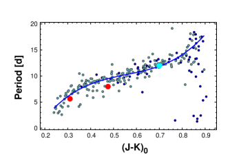
We show the three RV planets together with other known rotational variables on the (J$-$K) – period plane in Fig. 10. The rotational rates in the two clusters nicely follow the same pattern in the overlapping region of the main rotational ridge. This further confirms that the two clusters have the same age (Delorme et al., 2011). All three planet hosts are fairly close to the main ridge but the two in Praesepe may be slightly below it. When comparing with a similar plot for the Sloan r color (Fig. 4) we see that although the overall topology is the same, there are differences, attributed in part to the various noise properties of Sloan magnitudes and 2MASS color indices.

We tested various color combinations and appropriate transformations to stellar mass and temperature. They all gave very similar topology, albeit with different scatters. The status of both the cooler (Pr0211=HAT-269-0002316, $P_{\rm orb}=2.15$ d, $P_{\rm rot}=7.97$ d) and the hotter (Pr0201=HAT-269-0000805, $P_{\rm orb}=4.43$ d, $P_{\rm rot}=5.63$ d) planet hosts remained basically the same: the hotter one was always closer to (and likely to be on) the ridge, whereas the cooler one retained its relatively distinct position from the ridge. The planet host in the Hyades was also always close to the ridge but usually slightly on the short period side. When checking a similar plot of Meibom et al. (2011) for NGC 6811 (their Fig. 1b), we see that the two planet hosts have also slightly shorter periods than most of the stars at the same colors.

As far as Pr0211, the cooler planet host in Praesepe, is concerned, we find that the distance from the cubic polynomial fit to the ridge (see Sect. 3 and Table 3) varies between $-1.96$ and $-1.62$ days, depending on the color combination used. Although Pr0211 is certainly not the only one with similar deviations, the values quoted correspond nearly $20$% difference in rotational rate relative to ‘single normal’ stars, which we consider interesting enough to consider a possible relation between the faster rotation and the planet-hosting status.

If the cause of this difference is the angular momentum exchange between the planet and the host star, then from the models of Brown et al. (2011) we expect this system to be near (within a few hundred million years) to the end of its life time. Unfortunately, the implied decrease of the orbital period would still be under a small fraction of a second over a year, so it is not easy to verify this hypothesis by direct observations. On the other hand, the fact that the two other planet hosts, Pr0201 in Praesepe and HD 285507 in the Hyades sit closer to the respective ridge lines is in agreement with the expectation that in the case of these longer period systems the tidal interaction becomes far less important, and change their rotational periods with the same pace as other, ‘normal’ single stars.

The migration of HJs and their interaction with their host stars is obviously a very complex problem. This complexity is highlighted by the recent result of McQuillan, Mazeh & Aigrain (2013), who, based on the rotational analysis of $737$ planet host stars in the Kepler field, showed that fast rotation and short period planet hosting is a low probability event (see also Walkowicz & Basri 2013 and for a possible theoretical explanation Teitler & Königl 2014). We note however, that there are several/many HJ host stars in the field that rotate fast. For example (just selecting a few representative cases), from the published $V_{\rm rot}\sin i$ and $R_{\rm star}$ values one can easily derive that WASP-33 and KELT-1 are deeply within the ‘prohibited’ lower left corner of the $P_{\rm orb}$ – $P_{\rm rot}$ plot (see Fig. 2 of McQuillan, Mazeh & Aigrain 2013). The evolutionary ages are $0.4\pm 0.30$ and $1.75\pm 0.25$ Gyr, respectively. The age for WASP-33 is in agreement with the expected gyro age but for KELT-1 the gyro age is shorter by several factors. This indicates that KELT-1 rotates faster than expected for a single star with the same physical parameters. Other hosts, such as WASP-103, HAT-P-32, HAT-P-41, among others, are definitely below the border line of the $P_{\rm orb}$ – $P_{\rm rot}$ diagram, and, again, with multiple factors lower gyro ages as expected from the reasonably accurate evolutionary ages. These differences are large, even if we consider that there is a general inconsistency between the gyro and isochrone ages (e.g., Barnes 2009). The two hosts in Praesepe are at the border line, whereas the one in the Hyades is among the many other KOIs in the middle part of the diagram.

5 Conclusions

We analyzed $381$ high probability members of the galactic open cluster Praesepe and found that $47$% of them show significant variability, best understood as a consequence of the cyclic variation of the spotted area of the stars due to rotation. We found a fairly tight color/magnitude – period relation, in consonance with the earlier work of Delorme et al. (2011), based on a sample size less than a third of the one presented here. Our sample extends to the lower-amplitude variables at the hotter side, up to early F stars. This, and the dense coverage down to the late K regime, allows us to trace the nonlinearity in the color dependence of the rotational periods. Because of the high-rate sampling and wide color range covered by these data and because of the relatively accurate age of Praesepe, the derived color-period relation is well-suited for gyrochronological age determination (i.e., Skumanich 1972 and Barnes 2003).

We found a rather small number ($13$%) of the rotational variables with coherent light variation; most of them ($39$%) have residual power at the main rotational component and there are also many ($41$%) that have harmonic components. A relatively small fraction ($7$%) of them show separate but closely spaced frequency components, probably related to differential rotation. This latter type of variables are at the hotter, luminous end of the rotational sequence, whereas the ones with coherent single-period component are found preferably at the cooler (mid/low-luminosity) side. Each type of the other variables (the ones with unstable single component and those with harmonic components) cover uniformly the full color/magnitude range of rotational variables. The amplitudes show a broad range throughout the full span of color. An overall amplitude increase toward redder/fainter colors/magnitudes is also observable. However, this increase is largely attributed to the higher detection limits for those fainter stars.

From the two planet hosting stars the cooler one (Pr0211) has a rotational period that is $\sim 2$ days shorter than the one predicted by the main rotational relation at the given color in this cluster. Although there are several other – supposedly not planet host – stars with similar deviations, we may interpret this shorter period as a possible result of the exchange of angular momentum between the star and the planet at the expense of the planet’s orbital angular momentum. This inference is perhaps corroborated by the fact that the other planet (and also HD 285507 in the Hyades) are much closer to the corresponding ridge values. The planets in these systems have $2-3$-times longer orbital periods than the one in Pr0211, so we expect considerably weaker tidal interactions. Also, as discussed in Sect. 4, there are several Hot Jupiter planet hosts in the field that rotate faster than expected from their isochrone ages. The host of Pr0211 b could be one of these spun-up stars.

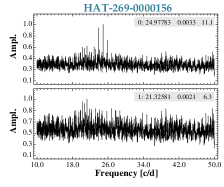
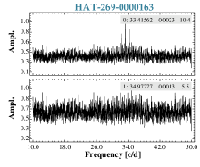
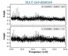
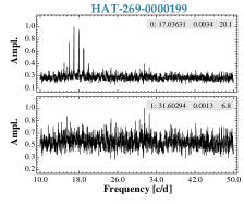
Appendix A Non-rotational variables

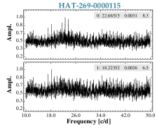
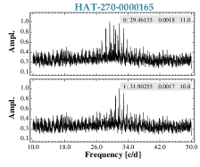
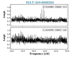
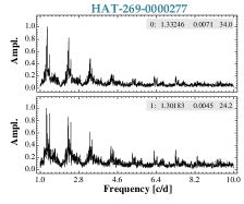
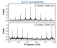
By following the methodology employed in the search for rotational variables, we searched for other types of variables among the $381$ high-probability cluster members (see Sect. 2.1). We found $10$ variables in the frequency range of [0,50]d^-1. Table 4 displays the most important properties of these variables. Figures 11 and 12 show the frequency spectra and the folded light curves for variables with frequencies greater than $1$d^-1. The case of HAT-269-0000465 is special. It is KW 495, a triple spectroscopic system (Mermilliod et al., 1994). Its frequency spectrum is rather complicated with two main frequency clumps at $\sim 0.079$ and $\sim 0.207$d^-1. The data are insufficient to classify this variable. Because of the detected period range, it is possible that the source of the signal is the rotation of two of the member stars. Alternatively, the complicated frequency spectrum and the late F (or early G) spectral type may suggest that this is a $\gamma$ Dor-type star.

In a technical note we mention that in several cases the application of TFA filtering was necessary for an unambiguous detection. Since the time series are the result of the merging of the data from the individual fields, and our main interest is to detect variability, we do not employ signal reconstruction as the second phase in the TFA filtering process (see Kovács et al. 2005). As a result, except for HAT-269-0000582, where the signal was stronger in the data before TFA filtering, the amplitudes are lower in the panels of Figures 11, than the ones listed in Table 4, where we used the original (EPD) data to compute the total amplitudes.

Most of the variables are known and classified as of $\delta$ Scuti type. We have probably 3 new discoveries (i.e., none of them are listed in the site of CDS nor mentioned in the current literature summary of this site on Praesepe). Star HAT-269-0000277 is most likely a pulsating variable with closely-spaced frequency components. This, together with the shape of the light curve, strongly suggests that this variable is a nonradial pulsator. The other object (HAT-270-0000165) is clearly a $\delta$ Scuti star.

Figure 11: Frequency spectra of the non-rotational variables with frequencies higher than $1$ d^-1. In each sub-figure the upper and lower panels show, respectively, the frequency spectra of the data and the spectra obtained after the first pre-whitening (with the peak frequency shown on the upper panel). The insets show the pre-whitening order, the peak frequency, the amplitude and the SNR of the peak.

It is interesting to compare the frequencies we obtained with those of Breger et al. (2012) derived from the data observed by the MOST satellite for the two variables common in these two studies. For BS Cnc Breger et al. (2012) detected 20 frequencies. We have good agreement for the main component: $(\nu_{0},{\rm Amp})=(17.0363,0.0062)$ for MOST and $(17.03626,0.0068)$ for HATNet (please note that our amplitude corresponds to the total signal amplitude - including also the [small] contribution of the other signal components). We also detected another component at $31.60299$ d^-1 with a much lower significance, at an amplitude nearly a third that of the main component. Interestingly, among the 20 components they found in the MOST data, there is the 10th component with basically the same frequency: $f_{10}=31.5988$. Breger et al. (2012) mention the puzzling nature of this component, since it was actually absent in their 2008 dataset whereas had a relatively large amplitude of $2.1$ mmag in 2009. Our data cover the period of December 2008 and June 2011 (with a large gap between May 2009 and November 2011). Therefore, it is likely that the amplitude of this component was still significant after 2009.

The variability of HD 73872 was discovered by the MOST satellite. Some $18$ components were detected, with the main component at $(\nu_{0},{\rm Amp})=(33.416,0.0030)$ and a second one at $(35.981,0.0025)$. We found a significant component at $33.41569$ d^-1 and a far less significant one as the second component at $34.97772$ d^-1. This latter one is very close to the $1$ d^-1 alias of the second component listed by Breger et al. (2012).

Table 4: Non-rotational variables in Praesepe detected in the HATNet database

HAT ID	2MASS ID	Other ID	$\nu$ [d-1]	K [mag]	J$-$K [mag]	A [mag]	SNR	Type
HAT-269-0000115	08420650+1924405	BX Cnc	22.6652144	7.431	0.114	0.0072	8.3	$\delta$ Scuti
HAT-269-0000156	08374070+1931063	BR Cnc	24.9778239	7.662	0.117	0.0078	11.1	$\delta$ Scuti
HAT-269-0000163	08411377+1955191	HD 73872	33.4156874	7.774	0.101	0.0054	10.4	$\delta$ Scuti
HAT-269-0000169	08405247+2015594	BW Cnc	14.8453080	7.804	0.107	0.0036	10.5	$\delta$ Scuti
HAT-269-0000199	08390909+1935327	BS Cnc	17.0362610	7.875	0.131	0.0068	20.1	$\delta$ Scuti
HAT-270-0000165	08452825+2023435	HD 74587	29.4613325	7.864	0.148	0.0039	11.0	$\delta$ Scuti
HAT-269-0000204	08403296+1911395	BV Cnc	32.9106985	7.964	0.119	0.0047	11.5	$\delta$ Scuti
HAT-269-0000277	08411067+1949465	HD 73854	1.3324437	8.190	0.174	0.0148	34.0	puls.?
HAT-269-0000465	08430593+1926152	BD+19 2087	0.2071673	8.461	0.333	0.0050	20.8	misc.?
HAT-269-0000582	08400171+1859595	TX Cnc	5.2235226	8.698	0.355	0.2983	61.8	EB

Notes: For variables with peak frequency $1<\nu<10$ [d^-1] the signal-to-noise ratio (SNR) is computed in the $[1,10]$ d^-1 band. For those with $\nu>10$ [d^-1], the $[10,50]$ d^-1 band is used. Amplitudes A [mag] are peak-to-peak values from the 4^th order Fourier fit to the instrumental Sloan “r” light curves, without TFA filtering. For the special case of HAT-269-0000465 the amplitude is a rough visual estimate of the total range of variation. For other details of this object, see text.

Figure 12: Folded light curves of the non-rotational variables found in the analysis of the $381$ Praesepe members with periods shorter than 1 day. For better visibility the folded data are binned in $200$ bins. The continuous line is the 3-rd (for HAT-269-0000582 the 5-th) order Fourier fit. The relatively large scatter in some cases is due to in part of the multiperiodic nature of these, mostly $\delta$ Scuti-type variables. Except for the upper two panels, the total amplitudes are smaller than those given in Table 4, since we used the TFA-filtered light curves without the reconstructive option.

Figure 13: Folded light curves of the four rotational variables that have close periods to the spectroscopic periods given by Mermilliod et al. (2009). For better visibility the data are binned in $200$ bins. The continuous line is the 3-rd order Fourier fit. The original (EPD) data are used, without TFA filtering.

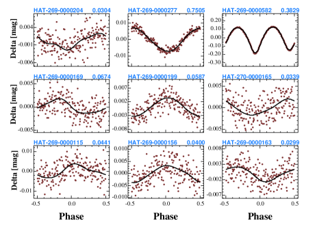
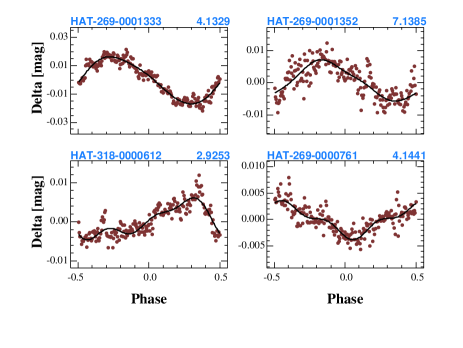
Appendix B Spectroscopic binaries

The status of the spectroscopic binaries (SBs) associated with the cluster has been summarized recently by Mermilliod et al. (2009). Based on their data collected by the CORAVEL spectrograph over a period of nearly two decades, they presented the orbital elements of 29 SBs. When we cross-correlate these stars with the $381$ stars selected from the overlap of the list of cluster members given by Kraus & Hillenbrand (2007) and the HATNet database, we get a list of $24$ stars. The spectroscopic (orbital) and photometric frequencies of these objects are shown in Table 5. The photometric frequency is the one that corresponds to the highest peak in the spectrum and does not necessarily agree with the finally adopted rotational frequency (see Table 2 for comparison). As discussed in the Sect. 6.1, the variable type of HAT-269-0000465 is unclear in spite of its high SNR.

We see that the orbital periods are, in general, much longer than the rotational periods. There are only three cases when we might face some ambiguity in distinguishing between the light variations caused by eclipses and by spots. However, inspecting the folded light curves does not lend too much support to the eclipse hypothesis, since they all seem to have distorted sinusoidal shape, with no resemblance of an eclipsing binary (see Figure 13). There is a fourth variable (HAT-269-0000761), which is an outlier in the color-period diagram with orbital and rotational periods differing by some $30$%. We could not find any trace of the orbital period in the photometric data. However, when we compare the photometric frequency with the one computed from the rotational velocity of $11.9$ kms^-1 (Mermilliod et al., 2009), we get $f_{\rm rot}=0.2547$ d^-1 (see Sect. 3.1 for details of the estimation of the necessary physical parameters of the star). This is in a very nice agreement with our photometric frequency.

Table 5: Spectroscopic binaries in Praesepe

HAT ID	KW ID	K	J$-$K	fphot	forb	forb/fphot	SNR
HAT-269-0000913	508	7.293	0.300	0.16167	0.00154	0.0095	22.9
HAT-269-0000528	47	7.353	0.338	6.28626	0.02889	0.0046	5.2
HAT-269-0000761	181	7.431	0.360	0.24131	0.17047	0.7064	23.1
HAT-269-0000489	268	7.610	0.259	0.58068	0.00693	0.0119	5.4
HAT-269-0000396	416	7.637	0.217	1.37448	0.03870	0.0282	5.0
HAT-269-0000726	3532	7.662	0.358	1.11693	0.02944	0.0264	3.5
HAT-269-0000465	495	7.769	0.333	0.21501	0.02786	0.1296	17.8
HAT-269-0000598	549	7.774	0.262	4.17972	0.03196	0.0076	5.9
HAT-269-0001333	434	7.790	0.383	0.24196	0.25428	1.0509	38.4
HAT-318-0000612	3655	7.804	0.422	0.34184	0.33537	0.9811	23.7
HAT-269-0001352	55	7.864	0.535	0.14009	0.16708	1.1927	22.0
HAT-269-0000767	287	7.875	0.363	1.45366	0.00014	0.0001	4.8
HAT-269-0000556	365	7.944	0.359	0.12007	0.01952	0.1626	7.2
HAT-269-0001570	368	7.946	0.430	0.11103	0.01306	0.1176	10.9
HAT-269-0000850	325	7.964	0.396	0.32065	0.00346	0.0108	8.5
HAT-269-0000287	142	8.044	0.241	0.37165	0.02175	0.0585	4.9
HAT-269-0000372	439	8.051	0.207	8.88541	0.00218	0.0002	4.8
HAT-269-0001402	539	8.063	0.396	0.26847	0.00018	0.0007	20.8
HAT-269-0000968	127	8.100	0.329	0.90909	0.07530	0.0828	6.2
HAT-269-0007340	536	8.190	0.873	0.58212	0.00079	0.0014	5.2
HAT-269-0000794	556	8.221	0.366	0.22052	0.00700	0.0317	26.2
HAT-269-0001490	184	8.351	0.502	0.09536	0.02108	0.2211	13.0
HAT-317-0001780	2025	8.369	0.503	0.20720	0.00038	0.0018	18.6
HAT-269-0003949	1184	8.377	0.660	9.57013	0.81290	0.0849	3.7

Notes: Photometric (f_phot) and orbital (f_orb) frequencies (in [d^-1]), respectively, are taken from this paper and from Mermilliod et al. (2009). The signal-to-noise ratio (SNR) refers to the peak frequency in the $[0,10]$d^-1 band, and is computed from the Fourier spectra of the TFA-filtered data. See text for more about f_phot and on the status of HAT-269-0000465.

References

- Agüeros et al. (2011) Agüeros, Marcel A. et al., 2011, ApJ, 740, 110
- Bakos et al. (2004) Bakos G. A. et al., 2004, PASP, 116, 266
- Bakos et al. (2010) Bakos G. Á. et al., 2010, ApJ, 710, 1724
- Balona et al. (2013) Balona, L. A., Joshi, S., Joshi, Y. C., Sagar, R., 2013, MNRAS, 429, 1466
- Barnes (2003) Barnes, S. A., 2003, ApJ, 586, 464
- Barnes (2009) Barnes, S. A., 2009, IAUS, 258, 345
- Boesgaard & Roper (2013) Boesgaard A. M., Roper B. B., 2013, ApJ, 775, 58
- Breger et al. (2012) Breger M. et al., 2012, AN, 333, 131
- Bressan et al. (2012) Bressan, A. et al., 2012, MNRAS, 427, 127
- Brown et al. (2011) Brown D. J. A., Collier Cameron A., Hall C., Hebb L., Smalley, B., 2011, MNRAS, 415, 605
- Brucalassi et al. (2014) Brucalassi A. et al., 2014, A&A, 561, L9
- Bouvier et al. (2013) Bouvier J. et al., 2013, arXiv1309.7851
- Canto Martins et al. (2011) Canto Martins B. L. et al., 2011, A&A, 527, 94
- Cargile et al. (2013) Cargile P. A., 2013, ApJ, in press, arXiv1312.3946
- Collier et al. (2009) Collier Cameron A. et al., 2009, MNRAS, 400, 451
- Deeming (1975) Deeming, T. J., 1975, Ap&SS, 36, 137
- Dékány & Kovács (2009) Dékány I., Kovács G., 2009, A&A, 507, 803
- Delorme et al. (2011) Delorme P. et al., 2011, MNRAS, 413, 2218
- Fossati et al. (2008) Fossati L. et al., 2008, A&A, 483, 891
- Franciosini et al. (2003) Franciosini E., Randich S., Pallavicini R., 2003, AdSpR, 32, 1143
- Gaspar et al. (2009) Gaspar A. et al., 2009, ApJ, 697, 1578
- Hartman et al. (2009) Hartman J. D. et al., 2009, ApJ, 691, 342
- Hartman et al. (2010) Hartman J. D., Bakos G. A., Kovács G., Noyes R. W., 2010, MNRAS, 408, 475
- Irwin et al. (2009) Irwin J. et al., 2009, MNRAS, 392, 1456
- Khalaj & Baumgardt (2013) Khalaj P., Baumgardt H., 2013, MNRAS, 434, 3236
- Kitchatinov & Olemskoy (2012) Kitchatinov L. L., Olemskoy S. V., 2012, MNRAS, 423, 3344
- Kovács et al. (2005) Kovács G., Bakos G. Á. Noyes, R. W., 2005, MNRAS, 356, 557
- Kraus & Hillenbrand (2007) Kraus A. L., Hillenbrand L. A., 2007, AJ, 134, 2340
- Lovis & Mayor (2007) Lovis C., Mayor M., 2007, A&A, 472, 657
- Mamajek & Hillenbrand (2008) Mamajek, Eric E., Hillenbrand, Lynne A., 2008, ApJ, 687, 1264
- McQuillan, Aigrain & Mazeh (2013) McQuillan A., Aigrain S., Mazeh T., 2013, MNRAS, 432, 1203
- McQuillan, Mazeh & Aigrain (2013) McQuillan A., Mazeh T., Aigrain S., 2013, ApJ, 775, L11
- Meibom et al. (2011) Meibom, S. et al., 2011, ApJ, 733, L9
- Meibom et al. (2013) Meibom S. et al., 2013, Nature, 499, 55
- Mermilliod et al. (1994) Mermilliod J.-C., Duquennoy A., Mayor M., 1994, A&A, 283, 515
- Mermilliod et al. (2009) Mermilliod J.-C., Mayor M., Udry S., 2009, A&A, 498, 949
- Messina & Guinan (2002) Messina S., Guinan E. F., 2002, A&A, 393, 225
- Noyes et al. (1984) Noyes R. W., Hartmann L. W., Baliunas S. L., Duncan D. K., Vaughan A. H., 1984, ApJ, 279, 763
- Penev et al. (2012) Penev K., Jackson, B., Spada, F., Thom, N., 2012, ApJ, 751, 96
- Pepper et al. (2008) Pepper J. et al., 2008, AJ, 135, 907
- Quinn et al. (2012) Quinn S. N. et al., 2012, ApJ, 756, L33
- Quinn et al. (2014) Quinn S. N. et al., 2014, ApJ, 787, 27
- Saar et al. (2011) Saar S. H., Dyke M., Meibom S., Barnes S. A., 2011, IAUS, 273, 469
- Sato et al. (2007) Sato B. et al., 2007, ApJ, 661, 527
- Scholz & Eislöffel (2007) Scholz A., Eislöffel J., 2007, MNRAS, 381, 1638
- Scholz et al. (2011) Scholz A. et al., 2011, MNRAS, 413, 2595
- Skumanich (1972) Skumanich A., 1972, ApJ, 171, 565
- Stetson (2000) Stetson P. B., 2000, PASP, 112, 925
- Stassun et al. (2002) Stassun K. G., van den Berg M., Mathieu R. D., Verbunt F., 2002, A&A, 382, 899
- Szulágyi et al. (2009) Szulágyi J., Kovács G., Welch D. L., 2009, A&A, 500, 917
- Taylor (2006) Taylor B. J., 2006, AJ, 132, 2453
- Teitler & Königl (2014) Teitler S., K nigl A., 2014, ApJ, in press, arXiv1403.5860
- Yuan et al. (2013) Yuan H. B., Liu X. W., Xiang, M. S., 2013, MNRAS, 430, 2188
- van Leeuwen (2009) van Leeuwen F., 2009, A&A, 497, 209
- Walkowicz & Basri (2013) Walkowicz L. M., Basri, G. S., 2013, MNRAS, 436, 1883
- Wang et al. (2014) Wang, P. F. et al., 2014, ApJ, 784, 57
- Zhang & Penev (2014) Zhang M., Penev, K., 2014, arXiv:1404.4365v2 (submitted to ApJ)