Key Elements of Robustness in Binary Black Hole Evolutions using Spectral Methods
Abstract
As a network of advanced-era gravitational wave detectors is nearing its design sensitivity, efficient and accurate waveform modeling becomes more and more relevant. Understanding of the nature of the signal being sought can have an order unity effect on the event rates seen in these instruments. The paper provides a description of key elements of the Spectral Einstein Code (SpEC), with details of our spectral adaptive mesh refinement (AMR) algorithm that has been optimized for binary black hole (BBH) evolutions. We expect that the gravitational waveform catalog produced by our code will have a central importance in both the detection and parameter estimation of gravitational waves in these instruments.
keywords:
Black holes; numerical relativity; Einstein’s equations; gravitational waves; spectral methods; adaptive mesh refinement.PACS numbers: 04.25.dg,04.30.-w
1 Introduction
A fundamental consequence of the field equations written down by Einstein, in his Theory of General Relativity, is the existence of singular solutions that are causally disconnected from remote observers. That is, surrounding the singularity will be an event horizon defined as the boundary of the region from within which a physical observer cannot escape. Astrophysical observations have lead to the realization that these objects are not only of theoretical importance. They are more than just the “point charge solution” of Einstein’s field equations. In fact, they are key players in how our universe functions. Given the large amount of observational evidence for the existence of black holes, it is a very natural question to ask – will these objects ever collide? If yes, what measurable quantities can be used to identify such an event. We know that galaxies collide (ours being one such “collided” galaxy). We know that galaxies host super massive black holes. Therefore black holes must collide as well.
The intent of this paper is to highlight some of the key elements of a particular numerical relativity code, the Spectral Einstein Code (SpEC), that allowed it to reach “production-level” in simulating binary black hole (BBH) mergers.
It is important to emphasize at a very early point in the paper that, though the current manuscript has a single author, the SpEC code is the result of years of work of a large number of people within what is known as the “SXS collaboration”. While a fair portion of the paper will be describing code contributions of the author, we will also make an effort to give due credit to all others involved.
Throughout the paper we will use Latin indexes from the beginning of the alphabet for space-time quantities, while will stand for spatial indexes. Partial derivatives will be denoted by while covariant derivatives will be written as .
2 Evolution System
2.1 The Generalized Harmonic System
Consider a spacetime metric tensor ,
| (1) |
The associated Christoffel symbol is defined as
| (2) |
We will refer to the trace of the Christoffel symbol as
| (3) |
The Einstein Equations, in a concise form, can be written as
| (4) |
where is the trace of the Ricci tensor which, in turn, is given by
| (5) |
An essential part of being able to numerically evolve a space time is to establish a well-posed initial boundary value problem. “Well-posed” here translates into saying that given some plausible initial and boundary data a unique solution will exist and that small perturbations in the freely specifiable data (on the initial slice or on the boundary) will result in small changes of the solution to the system under consideration. One approach to establish well-posedness of a system of partial differential equations is to show that the principal part (the terms containing the highest order derivatives) can be written as a first order symmetric hyperbolic system.
A careful look at the right-hand side (RHS) of Eq. (5) shows that the principal part consists of two terms: the wave operator acting on the metric and derivatives of (which itself consists of first derivatives of the metric). This, together with the identity
| (6) |
leads to the idea that one can think of as freely specifiable gauge freedom[1]. That is, rather than assigning values to each point of the manifold in some arbitrary (but smooth) way, one can think of the coordinates being determined indirectly through a wave equation
| (7) |
and regarding as freely specifiable. Specifying , with suitable initial and boundary conditions, is equivalent to specifying . Substituting into Eq. (8) gives
| (8) |
If the gauge source function is prescribed as a function of the coordinates and the metric but does not depend on derivatives of the metric,
| (9) |
then the sole term of the principal part of consists of the wave operator acting on the metric. This leads to a well-posed system, known as the generalized harmonic formulation of Einstein’s equations.
The identification induces a constraint in the generalized harmonic system, as is now a free function, while the trace of the Christoffel symbol is determined by derivatives of the metric resulting form the evolution equations. These equations are equivalent to the Einstein system only in the limit in which the constraint vanishes. It has been shown[2] that as a consequence of the Bianchi identities, the constraints propagate according to their own set of governing equations,
| (10) |
Thus the constraints themselves propagate as a set of coupled scalar waves implying that their evolution system is well-posed as well. This in turn means that small perturbations of the constraints in either the initial data or boundary data will not result in uncontrollable runaway solutions of the constraint system. In addition, the form of the source term of Eq. (10) tells us that for vanishing initial and boundary data on the constraints, they will remain zero in the entire evolved spacetime region.
In the actual numerical simulations constraint violating modes are generated at each time-step and on a variety of length-scales. Well-posedness is essential but not sufficient, as it does not exclude exponentially growing modes. Constraint propagation can further be improved by adding what is known as constraint damping terms to the evolution system. Given that the constraints are formed of first derivatives of the metric, one can add arbitrary combination of these (but not their derivatives) to the evolution system without modifying its principal part. A number of such terms have been proposed in the literature.[3, 4, 5, 6] The one employed by the SpEC code can be written as
| (11) |
where is the future directed unit timelike normal to the constant surfaces of the spacetime manifold, while is a free parameter.111In a typical BBH simulation we set to be a smooth function of coordinates, with in the inner region of the simulation and near the outer boundary of the computational domain.
2.2 Damped Harmonic Gauge
Next we turn our attention to various choices of the gauge source function . One immediate choice is to set the components of to zero, resulting in what is known as the harmonic gauge. Substituting this into Eq. (8) leads to the harmonic formulation of Einstein’s equations. Harmonic coordinates determine the fields by a wave equation and suitable initial and boundary values. In flat space this is feasible, as the ‘natural’ coordinates are trivial solutions of the wave operator,
| (12) |
In a non-trivial space time, however, in the presence of an actual gravitational potential, the scalar wave operator may amplify fields propagating under its action and form singularities. The net effect would be a singular coordinate system (with metric coefficients that become very large). Better choices are needed.
In his ground-breaking work, Pretorius [5] was able to use harmonic spatial coordinates but had to prescribe the time-component of the gauge source function by a damped wave equation that prevented the lapse function from collapsing to zero (which would be a signature of a singular time-coordinate). For generic binary black hole mergers, we found that better gauge choices are needed.
The current favorite gauge condition for binary black hole systems evolved with SpEC is the damped harmonic gauge[7, 8], described by
| (13) |
| (14) |
where is the determinant of the spatial 3-metric , is the lapse function and is the shift, defined as
| (15) |
The coefficients are used to control the amount of damping. We find that the choice
| (16) |
works well, where is a time-dependent coefficient that is rolled from zero to one in a smooth time-dependent way at the start of the simulation in order to reduce numerical error induced by initial gauge-dynamics of the BBH system.
Gauge conditions are intended to impose a condition on coordinates and, as such, they cannot be coordinate-independent (or covariant). This holds for our system as well. The form given in Eq. (13) acts a damping condition on the inertial frame222We define inertial frame the coordinate system in which the evolution equations are evolved. In these coordinates the far-field metric is a perturbation around Minkowski, while the coordinate position of the individual objects is time-dependent, as the black holes orbit each other. In a more precise sense, the inertial coordinates are determined by the initial and boundary data of the evolved metric quantities, along with our choice of harmonic gauge source functions defines the coordinates. damps the value of towards small values, effectively preventing the lapse from collapsing and/or the metric volume density from becoming very large.
The drawback of this gauge choice is that near merger, when objects tend to have larger coordinate velocities, it results in distortion. An alternative would be to impose the same condition in a comoving frame333The comoving frame, defined in Eq. (34), is the frame connected to the inertial frame by translation, rotation and scaling. In this frame the coordinate centers of the individual black holes are time-independent throughout the inspiral and plunge of the binary. Definition of a such frame is essential in our code as the underlying numerical grid is rigid, with fixed excision boundaries. These excision surfaces are kept just inside the dynamically evolved apparent horizons by the sequence of maps given in Eq. (33). (with coordinates ) of the binary.
When doing so, one has to be mindful of the fact that in general has transformation properties that depend on the particular choice of gauge condition (in our case Eq. (13)), while transforms as prescribed by its definition (see Eqs. (2)-(3)). As a consequence, naively substituting the co-moving frame metric quantities into Eq. (13) would not be what one might naturally think of as a corotating damped harmonic gauge condition. In order to clarify the meaning of the damped harmonic gauge in a particular frame, we start by observing that the quantity
| (17) |
is a tensor, where is a ‘background’ connection associated with some background metric . We can define the background in the inertial frame to be the Minkowski metric,
| (18) |
while the comoving background would be the tensor-transform of the inertial frame background metric into the comoving frame,
| (19) |
with Jacobian
| (20) |
The transformation of from the inertial to the corotating frame leads to
| (21) |
The co-moving damped harmonic gauge condition is
| (22) |
Substitution of Eq. (22) into Eq. (21) and expressing the result in terms of inertial frame metric quantities leads to
where and is the coordinate velocity of a comoving observer in the inertial frame. When compared to the inertial-frame variant of the same gauge condition, the term effectively makes the lapse condition milder early in the inspiral; the term damps the comoving frame shift to small values (rather than damping the inertial frame shift to small values regardless of the object’s velocity); and the last term is a consequence of the transformation properties of .
We have extensive experience with the inertial frame gauge condition. Whether placing this in the comoving frame helps is yet to be explored.
2.3 First Differential Order Form
Historically there has been a lot more know-how available for the analytic and numeric treatment of first differential order systems. Motivated largely by this reality, the main stream Generalized Harmonic evolution system in SpEC has been written in first order differential form[9]. This is done by introducing the auxiliary variables and defined by
| (24) | |||||
| (25) |
where is a free parameter. The resulting evolution system takes the form
| (26) | |||||
| (27) | |||||
| (28) | |||||
where and are additional free parameters of the system and we have included all terms, including the nonprincipal part.
The advantage of this system is that it is a manifestly first order symmetric hyperbolic system[9]. One of the drawbacks is that introduction of auxiliary variables leads to additional constraints for the system. The new constraint quantities are
| (29) | |||||
| (30) | |||||
| (31) | |||||
| (32) |
where full expressions for and are given in Ref. (\refciteLindblom2006). It has been shown[9] that the constraints associated with the extended, first order system form their own set of first order symmetric hyperbolic equations with source terms that vanish when the constraints are zero. By implication, given vanishing initial and boundary data for the constraints, the constraint propagation system will ensure that the constraints stay zero during the evolution. In addition, we find that, while the unmodified constraint propagation system may be prone to exponentially growing modes (seeded by numerical error induced at each time-step), the constraint damping terms are sufficient to control these growing modes for all cases of interest. Today, in all “production-style” binary black hole runs, we use the system given by Eqs. (26)-(28).
In parallel, as a side effort, a first differential order in time, second differential order in space version of the same system has been implemented and was shown to work well for a limited number of test-cases[10]. We expect that, if given enough effort, the second differential order form would be be at least a factor of two more efficient, given the smaller number of evolution variables the code requires. This approach has, however, received limited attention given the success of the first order system.
2.4 Boundary Conditions
One of the benefits of expressing a system in a symmetric hyperbolic form is that this formalism provides a way of identifying the main characteristic speeds of a system across a given boundary, as well as the associated characteristic fields. This then leads to an easy-to-follow recipe for constructing boundary data. One must provide data for those quantities that are incoming through the boundary, while making sure that the outgoing quantities are updated through their evolution equations (and thus allowed to naturally leave the domain). An additional criteria is that the incoming data must not be specified in a way that injects constraint violating modes. There are a number of versions of constraint preserving boundary conditions for the generalized harmonic system. Most notably, Kreiss and Winicour has worked out a geometrically motivated, well-posed boundary system in Ref. \refciteKreiss2006,Babiuc:2006ik,Kreiss:2013gw.
The SpEC code implements a boundary algorithm based on Rinne, Lindblom and Scheel[9]. The current algorithm works well for BBH evolutions of up to a few dozen orbits. However, it becomes a major limitation in evolutions lasting hundreds of light-crossing times – in these simulations our current boundary algorithm acts as a gravitational potential, causing an acceleration of the center of mass. The well-posedness and stability of this evolution-boundary system has been studied by Rinne in Ref. \refciteRinne:2006vv.
3 Domain Construction
One key element influencing the design of the spectral domain used in the SpEC binary black hole simulations is the choice to use excision as a means of dealing with the space-time singularity inside the horizon. Finite difference codes have been successful in BBH evolutions with[5, 15] and without excision[16, 17]. While an excision-less domain is much easier to construct and an excision-less evolution algorithm is much less involved on a technical level than one with excision, spectral accuracy would be lost if the evolution field had nonsmooth features. The singularity would introduce such nonsmoothness, even if one factors out and regularizes the singularity (e.g., by evolving the conformal metric and the inverse of the conformal factor, as done in some of the puncture codes). As a result, in SpEC the computational domain needs to accommodate two inner spherical excision boundaries. In addition, the most natural outer boundary shape is spherical as well, which is easily accommodated by the wave-zone spherical grid used in our code.
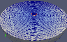
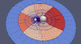
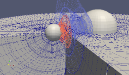
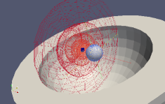
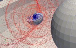
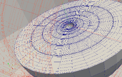
After a number of attempts at the problem of domain construction, we have settled on the non-overlapping domain described in the Appendix of Ref. \refciteBuchman:2012dw. This grid is composed of a small number of spherical shells around each excision boundary, labeled as SphereA and SphereB, where (see Fig. 3). The innermost of these sets of spherical shells, also referred to as the excision subdomain, has index zero. In addition, the grid contains a third set of shells describing the gravitational wave zone (shown in Fig. 1), labeled as SphereC, . In a typical simulation we have outer shells. The space between the innermost outer shell, SphereC0 and the outer boundary of the inner shell structures is filled up by a set of cylindrical subdomains, distorted both on the lower and upper end, so that they touch their neighboring subdomain (shown in Fig. 1, and Fig. 2). The space between the two inner sets of spherical shells is filled in with another set of distorted cylinders which, on one end, are touching the spherical boundary of the outermost of SphereA and SphereB, while on the other end they touch an const grid-plane, referred to as the CutX plane, as shown on Fig. 2.
In conjunction with inter-block penalty boundary conditions and appropriate spectral filters (see Sec. 5), a major advantage of our current compact binary grid is its robust stability with respect to high frequency noise generated by our numerical update scheme. This is a non-trivial property of a spectrally evolved BBH system where high accuracy leaves room for very little numerical dissipation. In addition, we find our domain to adapt well to binaries with very different masses.[19, 18]
The domain construction (or control of its parameters) requires an extra amount of care near the merger of the binaries. This is to be expected, as BBH simulations tend to spend the longest amount of physical and wall-clock time in the inspiral phase. During this phase, little changes as the black holes slowly approach each other, while radiating energy via gravitational wave emission. It makes most sense to design a grid that does well during the early stage. As the binary approaches merger, the excision boundaries (kept in the near vicinity of the individual apparent horizons) approach each other. It is essential that all features of the grid are able to adjust to this deformation. In order to avoid grid singularities (or noninvertible maps, as described in Sec. 4), at various stages during the plunge our algorithm defines a new grid, with modified parameters such that the position of the CutX plane remains between the spherical shells around the excision boundaries until after merger. See Secs. 6.3 and 6.2.1 for details.
4 Control System
As mentioned earlier, the SpEC code uses excision for evolving systems involving black holes. This creates its own set of challenges. In a finite difference code, in order to properly excise the interior of a black hole, one needs to locate the apparent horizon and implement an algorithm with a moving excision boundary. As the black hole moves on the grid, there will be grid-points that are evolution points on one time-step which become excision points on the next time level. In addition, there will be other points that are labeled as excision points at some time only to become evolution points as the black hole moves past them. This can be implemented on a point-wise basis, as has been done in a number of finite difference codes, e.g. in Ref. \refciteSzilagyi2007. In a spectral algorithm the removal of a single grid-point is not feasible as, in some sense, spectral differencing stencils are global within the subdomain (or block). As a result, there is no option to move an excision boundary along a particular direction by one grid-point. Rather, we employ a feed back control system[20] based on measurement of the position of the black holes, which rotates, translates and shrinks the grid such that the coordinate centers of the excision boundaries tightly follow the motion of the coordinate centers of the apparent horizons. In addition, we monitor the coordinate shape of the apparent horizons in the co-moving frame and apply a distortion map to the excision boundary such that it stays just inside the apparent horizon throughout the evolution, including plunge and merger. The full sequence of maps employed in a BBH evolution is given by[20] , where are inertial coordinates, are grid-frame coordinates, and
| (33) |
Here
-
•
is a spatial map which translates the mass-weighted average of the centers of the excision boundaries so that this point is in the neighborhood of the coordinate-center of mass of the BBH system as it evolves. This map leaves the position of the outer boundary unchanged.
-
•
rotates the grid such that the line connecting the centers of the excision boundaries is aligned with the one connecting the coordinate centers of the apparent horizons.
-
•
shrinks (or expands) the grid at the right rate such that the distance between the centers of the excision boundaries is synchronized with the distance between the coordinate centers of the apparent horizons. This map is also responsible for a slow inward motion of the outer boundary so that constraint violating modes with vanishing characteristic speed leave the domain rather than stay forever.
-
•
is responsible for distorting the CutX plane at late times, when the excision boundaries are near each other, such that this skewed grid plane stays at a finite distance from the excision boundaries even when they are non-perpendicular to the axis. See Figure 3 in Ref. \refciteHemberger:2012jz
-
•
is responsible for controlling the position of the CutX plane (by moving along the axis) such that it remains at a finite distance from the point where the excision boundaries cross the axis. See Sec. 6.3 as well as Ref. \refciteHemberger:2012jz for details.
-
•
is responsible for deforming the excision boundary from its original spherical shape to that of the apparent horizon.
In Sec. 2.2 of the paper we made reference to the comoving frame (with coordinates ) defined as the frame in which the coordinate centers of the apparent horizons are at a fixed position. This frame is connected to the inertial frame by the map
| (34) |
leading to
| (35) |
Another frame of relevance is the distorted frame , connected to the grid-frame coordinates by
| (36) |
giving
| (37) |
This is the frame in which we search for the apparent horizons, feeding it into the control system responsible for updating the time-dependent parameters of the various maps. In terms of the maps associated with the distorted and the comoving frames the full transformation from the grid frame to the inertial frame can then be written as
| (38) | |||||
| (39) |
Note that for the inspiral part of our BBH simulations, where is inactive, the distorted frame is simply the grid frame distorted under the action of the shape-map . Also, note that the comoving frame and the distorted frame differ by the skew-map . The motivation of working with two different though similar frames is in their use. The comoving frame is instrumental in defining a gauge condition, as described in Sec. 2.2. The distorted frame is introduced for the sake of a more convenient implementation of our grid-control algorithm; thus its definition is more naturally stated through its relationship to the grid frame.
5 Pseudo-Spectral Numerical Algorithm
The irreducible topologies at the core of our grid construction are
| (40) | |||||
| (41) | |||||
| (42) | |||||
| (43) |
The computational domain for binary black hole simulations is built of blocks that are topologically
| (44) |
The spectral basis is associated with the irreducible topologies is, in order, Chebyshev polynomials, Fourier expansion, scalar spherical harmonics and one-sided Jacobi polynomials. Each of these come with their set of collocation points so as to optimize the conversion between collocation point data and the spectral coefficient representation. Our algorithm stores collocation values of each evolved quantity, at a given time-step.
Derivatives are computed by forming the spectral coefficient representation of the same data and then recombining those with the analytic derivatives of the spectral basis functions. For example, given some smooth function we approximate it as an expansion in terms of a spectral basis ,
| (45) |
The derivative of the function will then be approximated by
| (46) |
where the derivatives of are known analytically.
Given the nonlinear nature of the evolution system of interest, we find it easier to compute the RHS of the equations, at each collocation point, using the actual function values (rather than their spectral coefficients). The nonlinearity implies coupling between neighboring coefficients. By implication, the highest coefficients of any given representation will effectively be updated by the “wrong equation.” In other words, their effective update scheme depends on whether there exists a higher coefficient in the data or not. In some cases this is not a problem since, for well-resolved, exponentially convergent representations of a smooth evolved field, the highest coefficient may already have a very small magnitude so that having (or not having) a next higher coefficient would have no appreciable impact on the evolution of the field. In order to achieve robust stability, we find that, we must filter these higher coefficients. In particular, after each time-step we set the highest four coefficients of the expansions to zero[21],
| (47) |
where is the Heaviside step-function. In addition, we use the exponential filter
| (48) |
with for the Chebyshev coefficients, as suggested in Refs. \refciteGottlieb2001 and \refciteHesthaven2007. We use the same exponential filter for the Fourier coefficients as well, using , though in this case our choice is entirely heuristic. These filters are applied to the evolution variables after each full time-step. In addition, each time one subdomain provides boundary data to another via interpolation, this interpolated data is filtered using the Heaviside filter Eq. (47) for the scalar spherical harmonic expansions on type boundaries and the exponential filter Eq. (48) for all Chebyshev and Fourier expansions. For those boundaries, where the neighboring collocation grids are aligned at the boundary, there is no need for interpolation. In these cases we are copying the data from one subdomain to the other without any filtering. Having the right filtering scheme proved crucial in being able to establish robust stability.
5.1 Accuracy Diagnostics
Exponential convergence of the spectral representation of smooth data in a particular basis requires that, for sufficiently large mode number, the expansion coefficients are exponentially decaying functions of the mode number. As an example, for a smooth function on an surface, the spectral expansion in terms of scalar spherical harmonics is
| (49) |
When the function is well resolved, then the magnitude of the highest order coefficients will decay exponentially,
| (50) |
This suggests that one should monitor the quantity
| (51) |
in order to asses the accuracy of the spectral representation. This is done in a more generic context. Whenever dealing with tensor products of irreducible topologies, we monitor accuracy of the representation by computing the average (in an sense) over all other dimensions; e.g., for , we define power-monitors according to the three indexes, as
| (52) |
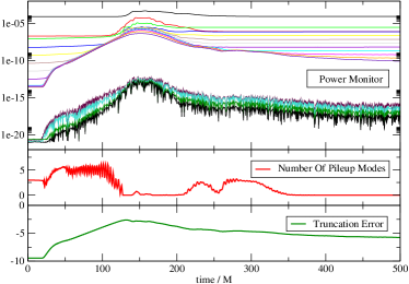
with similar definitions for . A time-snapshot of an example power-monitor plot is provided in Fig. 4. A few key features are immediately noticeable. The highest mode has roundoff power, which results from filtering. The lowest six modes (or: the first six, counting from the left) in Fig. 4 show a clean exponential decay. This is indicative of exponential convergence, and allows us to define the convergence factor as the logarithmic slope of the power in the coefficient vs. its index. The ratio of the highest to the lowest coefficient in this clean convergent set of points gives a measure of the truncation error in the expansion. And the few extra modes that are placed between the convergent modes and the filtered mode are labeled as “pile-up modes.” These indicate saturation of the grid with respect to the data that is being spectrally expanded. They are most likely related to noise in the data, possibly due to non-smooth boundary data on the subdomain boundary.
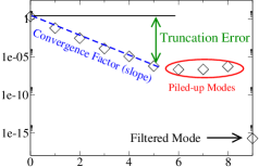
For spectral Adaptive Mesh Refinement (AMR), it is important to define all of these quantities as smooth functions of the power monitor values . Let be the slope of the least square fit of for the points , with . Let be the error in this fit. In our current algorithm we first compute and for a variety of selections of data points. Then we define the convergence factor (up to an overall negative sign) as the average of the slopes, weighted by the inverse of their fit error,
| (53) |
where is a small positive constant to avoid division by zero in case the linear fit has no error, while is the number of unfiltered modes, with . Note that for some of the filters, in particular for the scalar filter used in the evolution of tensor fields, the filtering algorithm amounts to setting the highest few coefficients to zero, as shown in Eq. (47). In this case the number of filtered modes would equal the number of those coefficients that are being reset. In the case of the exponential Chebyshev filter Eq. (48) we approximate the number of filtered modes as those whose coefficient is below some threshold, e.g., it is roundoff. By calculating a large number of fits and weighting them by the inverse of the accuracy of the fit, we give the larger weight to those sets of points that provide a clean slope. This is important on both ends of the spectrum. For the lower order modes one cannot expect, generically, a particular behavior (such as exponential decay) as we look at the spectral expansion of an arbitrary (smooth) function.444 For instance, the space-time metric in the weak field region (such as the neighborhood of the outer boundary in a typical binary black hole simulation) has the form (54) (where is the Minkowski metric). In this case the lowest order coefficient corresponding to the constant element of the expansion basis will be while all higher coefficients will be several orders of mangitude smaller. Resolving the perturbative part of the metric in this wave zone is essential, as this is the effect we are trying to capture and translate into the signal seen by a gravitational wave detector. The convergence factor estimate would be incorrect if it included the part coming from the flat space metric . The highest modes may be tainted by noise (they could be pile-up modes) which, again, would lead to inaccurate measure of the convergence factor. This algorithm also gives some level of robustness when certain coefficients show anomalies (e.g. because the data has some excess power in a given spectral mode). An example power-monitor (as a function of time), along with the associated convergence factor computed using Eq (53), is given in Fig. 5.
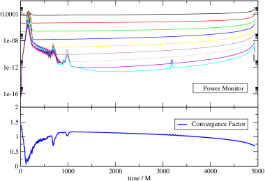
Pile-up modes are identified by a local convergence factor estimate, involving the mode under consideration and its next few higher neighbors. Once again, the AMR algorithm benefits from a pile-up mode counter that is a continuous function of the data (rather than a discrete counter). In order to measure the extent to which a given mode is a to be considered as a pile-up mode, we measure a local convergence factor around the -th point,
| (55) |
and compare it to the overall convergence factor, . The number of pile-up modes is then defined to be
| (56) |
If the local convergence factor estimate associated with the mode has a value close to that of the overall convergence factor, i.e. if
than that mode will have an roundoff contribution to . If it is near zero, i.e.,
this indicates that we are down in the noise floor of the power-monitor plot, and the contribution of the individual mode to the number of pile-up modes will be . A plot showing the number of pile-up modes, and the associated power monitor, for a typical BBH production run is shown in Fig. 6.
A third quantity essential in our spectral AMR algorithm is the truncation error estimate associated with the power-monitor . This is computed using the expression
| (57) | |||||
| (58) |
The aim here is to count the number of digits resolved by the given set of spectral coefficients. This is computed as the difference between the power in the larger of the two lowest order modes, , and the power in the highest modes, which itself is computed as an exponentially weighted average, giving maximum weight to the last two points (refer to Fig. 6).
The truncation error , the convergence factor and the number of pile-up modes are the three essential measures that our AMR algorithm relies upon.
6 Adaptive Mesh Refinement
In finite-difference based discretization schemes one commonly used AMR algorithm is that described by Berger and Oliger in Ref. \refciteBerger1984. In such a scheme the evolution would be done on a sequence of refinement levels simultaneously. The truncation error between the two highest refinement levels can then be used to monitor the accuracy of the evolution and to dynamically assign the number of refinement levels to a particular region of the grid. Each refinement level will have a factor of two smaller grid-step (and possibly time-step) than the next coarser level. For a region that has refinement levels at a particular instant of time, there will simultaneously co-exist the highest level, the coarser one, the next coarser one, to the coarsest, all used to discretize this region at varying levels of accuracy.
Our approach to mesh refinement is different. The SpEC code uses a single layer of grid for a given (BBH) simulation. On a very basic level, our mesh refinement algorithm monitors the truncation error estimates associated with each irreducible topology, within each subdomain, throughout the run and then adjusts the number of collocation points (and, accordingly, the number of spectral basis elements) in order to keep the local truncation error within some desired range. This is called -type mesh refinement.
In addition, as the objects approach each other while on their trajectories, our control system and the associated maps shift the boundaries of the various subdomains with respect to each other in order to accommodate the requirement that the excision boundary must stay inside the apparent horizons at all times. As a consequence, from time to time subdomain boundaries need to be re-drawn in order to reduce the stretching or compression of the grid caused by their continuous drifting under the action of the various maps. When this change of the grid structure implies splitting or joining of subdomains, we call this as -type mesh refinement. When it preserves the number of subdomains but shifts their boundaries, it is called -type mesh refinement. In addition, our AMR driver splits subdomains when the number of spectral modes required for a given target accuracy exceeds some threshold. This happens regularly with the spherical shells surrounding the smaller black hole in high mass ratio mergers, and is another example of -type mesh refinement in our code. In the following sections we give a description of each of these elements of our AMR algorithm.
6.1 -type mesh refinement
To zeroth order the -type mesh refinement algorithm monitors the truncation error estimate for each power-monitor associated with the individual subdomains, and adjusts the number of collocation modes (by adding or removing modes) such that the accuracy of the spectral representation of the evolved quantities is within some desired range. This behavior is seen on Fig. 7. The algorithm behind the plot contains additional elements described in the remainder of this section. Nevertheless, the plot is a good illustration of how -type mesh refinement works in our code.
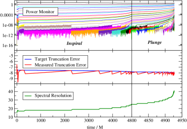
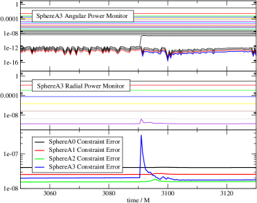
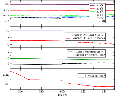
Each time a basis associated with a particular subdomain is extended, we find that the numerical evolution system needs some time to adjust and find a new quasi-equilibrium for the evolved coefficients. This can be seen both in the power-monitors and in the constraints, as shown on Fig. 8. For this reason, our current algorithm calls the AMR driver at pre-set time-intervals (rather than every time-step). Each time a particular grid extent is changed, it will be kept at the new level for some time before it is allowed to change. During the early inspiral, grid extents are changed no more frequently than every evolution time. This time-interval is gradually decreased and during the plunge individual grid extents are allowed to change every . An alternative way of dealing with this same problem would be to use a smooth filter for all spectral expansions and control the parameter of this filter as a continuous function of time so that when the AMR driver decides to remove a point the filtering coefficients gradually become stronger for the highest unfiltered coefficient, until it reaches roundoff level. At this point the highest coefficient could be safely be removed (as it could only gain power from coupling to the next highest coefficient which by now is also filtered) and doing so would not present a noticeable ‘shock’ to the numerical evolution scheme. A similar approach could be applied for adding a new spectral coefficient. Implementation of such a ‘smooth’ resolution change is future work.
6.1.1 Target truncation error
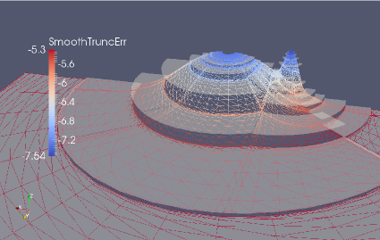
An important element in the robustness of our current AMR algorithm is the proper setting of the target truncation error. An essential requirement on the angular resolution of the spherical shells is that they must be able to represent the data at a level accurate enough for the needs of the horizon finder. The horizon finder, however, does not depend only on the angular representation of the data. Radial resolution is required as well. Another important physical aspect that we want to represent accurately in our simulation is the amplitude and, more importantly, the phase of the gravitational wave (as gravitational wave detectors are more sensitive to phase than amplitude). In the outer layers of the grid, these waves propagate as outgoing spherical wavefronts, which do not require a lot of resolution. It is important, however, to get the orbital phase of the binary right, since if the orbits are inaccurate then the waves (generated by the motion of the black holes) cannot be accurate either. For the sake of simplicity, we use the label ‘A’ for the black hole contained in the subdomains SphereA and ‘B’ for the black hole contained in the subdomains SphereB. In the region immediately surrounding the black holes (including the subdomains discretizing their gravitational attraction between the two excision boundaries), we find that we need higher accuracy. Our target truncation error function is written as
| (59) |
where the weighting coefficients are the norm on each subdomain of the smooth weight functions
which are expressed in terms of inertial coordinates , with maximum values around the time-dependent coordinate-center of the individual black holes labeled ‘A’ and ‘B’:
| (60) | |||
| (61) |
Note that here we use the initial distance of black hole ‘A’ to the coordinate origin to set the falloff rate of the Gaussian controlling the truncation error requirement around black hole ‘B’, and vice-versa. The rationale is that if one black hole is larger, it starts off closer to the origin, i.e., the other smaller black hole will have a smaller Gaussian around it. As a further constraint on , this quantity cannot differ by more than between two neighboring subdomains. This rule is enforced by setting stricter truncation error on those subdomains that otherwise would end up being coarser than intended. We plot both the subdomain-wise constant and the smooth function in Fig. 9.
6.1.2 Special rules for spherical shells
In order to control the accuracy of the apparent horizons themselves (and, as such, of the numerically evolved black holes), we define three criteria that factor into the final choice of the angular resolution of the horizon finder:
-
1.
We form a expansion of the shape function of the horizon surface, which is defined as the coordinate distance between the point on the surface and its coordinate center.555Note that the angular coordinates are defined local to the horizon center and are independent of where the horizon is located with respect to the global coordinate-systems center. Given this spectral expansion, we form a power monitor Eq. (51) and then compute the truncation error estimate Eq. (58) and the number of pile-up modes Eq. (56). If the surface shape is coarser than required and if the number of pile-up modes is not larger than some threshold, we increase the accuracy of the horizon finder. If the number of pile-up modes is already at its limit, adding more modes would not help.
-
2.
As a second method of determining adequacy of resolution, we form a expansion of the areal radius of the apparent horizon surface and require that it be represented with a truncation error that is within a desired range. Note that the surface areal radius will reduce to the coordinate radius in flat space time. Imposing an accuracy requirement on the surface areal radius requires an accurate representation of the metric quantities on the horizon surface. This in turn allows for accurate measurement of physical quantities such as areal mass and spin. Similar to the coordinate radius, the horizon finder will increase accuracy if the areal radius is under resolved (and does not have too many pile-up modes).
-
3.
As yet another method for imposing an accuracy requirement on the horizon finder algorithm, we monitor the residual of the horizon finder. If larger than requested, the angular resolution is increased.
If the accuracy of the surface is better than required by any of these measures, the horizon finder will decrease accuracy.
The angular resolution of the horizon finder can be used to set a lower limit on the angular resolution of the underlying three-dimensional evolution grid. Given the top-4 Heaviside filters Eq. (47), we request that the set of spherical shells around the excision boundary associated with a given horizon must have five additional modes beyonf the surface finder’s resolution. This implies that, should any of the horizon finder accuracy criteria request higher resolution, additional data is available upon interpolation from the evolution grid. Once the horizon finder increases its resolution, the spherical shells around its excision boundary have their angular resolution increased.
The angular resolution of the horizon finder is a useful lower limit for the spherical shells around an excision boundary. There are additional, heuristic rules that we found useful not only for accuracy but also for well behaved constraints.
The first such rule is that given the angular resolution of a spherical shell subdomain, its neighbors must not have angular resolutions larger than or smaller than . There is yet another heuristic rule relating the angular resolution of the excision subdomain to the spherical shells surrounding it. As the binary system evolves, the further a subdomain is from the excision boundary, the less spherical symmetry will be in the metric data. Based on truncation error estimates, this means that the AMR driver will assign larger angular resolution to the spherical shells that are further from their associated excision boundary and closer to the other black hole. In certain cases, however, the metric data on the excision boundary may itself require a large resolution (e.g., if the black hole has a very large spin or distortion). When the subdomain next to the excision boundary has a larger angular resolution that its neighbors, we find that the constraint errors grow on a short time-scale. This may be related to the fact that if a given subdomain boundary has subdomains of different resolution on its two sides, those angular modes that are represented on only one side of the boundary will be reflected. When the excision subdomain needs high resolution, it may also be responsible for a larger amount of high frequency noise generation. If this is the case and its neighbor has a lower angular resolution, all that noise can get trapped in the excision subdomain and have non-desired effects on the black hole itself. Thus, to rule this out, if the excision subdomain needs resolution then all its neighbors are given the same, or larger, resolution.
The angular resolution of the set of shells resolving the wave-zone is driven by a much simpler set of rules. In this region we base the angular resolution of the shells on the truncation error estimate Eq. (58) derived from the power-monitor associated with the scalar expansion of the main evolution variables . Similar to the inner sets of shells,we do not allow neighboring wave-zone shells to have their angular resolution differ by more than one . As a possible future improvement, it may be worth forming a power-monitor from the spherical harmonic decomposition of the Weyl scalar and require that the truncation error associated with this power-monitor also be within limits.
6.1.3 Pile-up mode treatment
An essential element of our Spectral AMR algorithm is the treatment of pile-up modes. The source of these modes is not fully understood, although we expect that inadequate filtering or unresolved high frequency modes injected through a subdomain boundary can lead to such modes. It is also expected that, when the evolved quantities have a lot of non-trivial features, a more fine-grained definition of the truncation error estimate Eq. (58), convergence factor Eq. (53) and pile-up modes Eq. (56) could prove helpful in better tracking and controlling the numerical representation of the evolved quantitites.
As seen in Fig. 4, the presence of these pile-up modes does not contribute to the accuracy of the data. On the contrary, we find in practice that these modes are constraint violating modes. This suggests that pile-up modes are result of the numerical approximation and not a property of the underlying analytic system. In other terms, Einstein’s equations will likely not dictate the presence of such modes. Rather, these develop on the grid as a result of limitations of our particular numerical scheme. We do not have experience with other spectral evolution codes and therefore are unable to assess whether these modes are a generic property of spectrally evolved partial differential equations. In our experience, however, the less pile-up modes, the better. For this reason we make it a priority to eliminate them, or to prevent their creation.
One immediate way of handling pile-up modes is to remove them. If a power-monitor shows these modes, we simply reduce the grid-extent associated with the piled-up power-monitor. In some cases doing so would violate some of our other rules of thumb (e.g., the horizon finder may need a certain minimum resolution). In this case we keep the resolution of neighboring subdomains from increasing until the pile-up modes leave the grid either by filtering or by propagating away from the subdomain under consideration. Fig. 10 illustrates, what we find in most cases, that removal of pile-up modes helps reduce the constraint violating modes on the grid. This suggests that these modes do not result from the underlying analytic system but are instead a numerical artifact.
6.1.4 AMR driven by projected constraint error
As an alternative way of determining whether a given grid extent needs to be changed, one can monitor the constraint quantities , defined in Eqs. (31),(29). The first of these indexes are related to derivatives, while the rest of the indexes are related to the evolution frame of the main system (i.e., the inertial frame). In order to derive an accuracy requirement based on the constraints, we make use of the fact that each subdomain is constructed as a product of topologies (see Eq. (44) for a list of these topology products). We form an estimate of the contribution of the truncation error associated with the individual topologies by projecting the derivative indexes from the evolution frame into the frame associated with the topology product that is used to construct the grid .
That is, for a spherical shell, we project the Cartesian index of onto spherical coordinates, summing over the non-derivative indexes. In general, we write
| (62) | |||||
| (63) |
where the normalization coefficient is set using
| (64) |
The or the norm of and over the individual subdomains can then serve as an indicator of whether the spectral expansion associated with the topological coordinate has an adequate accuracy. We have tested this algorithm in conjunction with the truncation-error based AMR described in Sec. 6.1.1, always applying the stricter of the two requirements. We find that this additional accuracy requirement can be helfpul in the more dynamic parts of the BBH simulation (such as during plunge) where constraint violating modes can develop faster and spoil the physical properties of the system.
6.2 -type mesh refinement
In a general spectral AMR algorithm, -type mesh refinement is motivated largely by efficiency considerations. If it takes too many spectral coefficients to resolve data along a particular axis of the subdomain then differentiation may become very expensive, the time-step may be limited due to a stricter CFL limit, memory limitations may arise, and load balancing may become a problem if the application is parallelized. All of these concerns are relevant for our code as well. We monitor the convergence factor Eq. (53) of a given power-monitor and when it reaches values below some arbitrary threshold, the subdomain will be split. In our binary black hole evolutions typical values for the convergence factor are of order unity, so our threshold for splitting is set to . In addition, we find it useful to set hard limits on the maximum number of spectral coefficients allowed for a specific irreducible topology of a give subdomain type. For instance, our rule is not to have more than 20 radial points in any spherical shell. If the -type AMR driver finds that this number is not sufficient then the subdomain will be split in the radial direction.666One such scenario, found in a number of our binary black hole inspirals, is the radial splitting of some of the outermost spherical shells. This results from the action of the cubic scale map , which is responsible for shrinking the interior of the grid as the binary approaches merger, while some of the outer subdomains get stretched. The AMR driver monitors this through the truncation error of the radial spectral expansion and keeps adding coefficients until the user-specified limit of the maximum allowed radial collocation points is reached. Then the subdomain gets split and the evolution can proceed.
Another role of the -type AMR in our runs is around the individual excision boundaries. For a number of our binary simulations one of the apparent horizons will pick up more and more angular resolution, forcing the underlying spherical shells to add spherical harmonic coefficients with higher and higher values of . When the angular resolution reaches a user-specified limit, the spherical shell is split. We find it important that when such a spherical shell is angularly split, all shells outside it (among those around the same excision boundary) be split as well. This, once again, is a rule we found useful by trial and error when optimizing for small constraint violation.
6.2.1 Shell-dropping around the excision boundaries
What we call our ‘shell dropping algorithm’ is a use of -type AMR which is an absolute must in our binary evolutions.
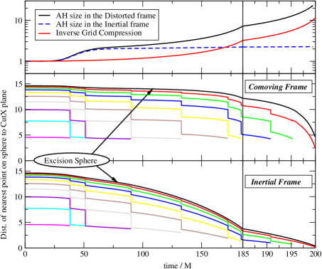
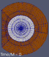
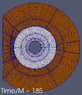
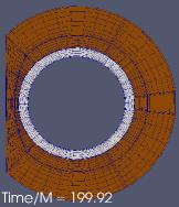
As the black holes approach each other, the ratio of the size of the excision boundaries and the distance between their centers will grow. In the co-moving frame, where this distance is fixed by definition, the signature of the plunge is that the apparent horizons (and the excision boundaries within them) go through a rapid growth. Our implementation of the shape map is such that the various spherical shell boundaries around a given excision boundary stay at a constant distance from one another. As the excision boundary grows, this causes the outermost spherical shell to approach the plane cutting between the two sets of spherical shells, as seen in Fig. 11. In order to prevent a grid singularity, when this condition is detected, we re-draw the computational domain, typically reducing the number of spherical shells around the excision boundary by one. When we do this, we also optimize the radii of the remaining shells so that they form a geometric sequence in the co-rotating frame. This is done several times as the black holes approach each other. Near merger typically one would have a single spherical shell left around the excision boundary of the larger hole (see the right panel of Fig. 12), as this is quicker to approach the cutting plane. Especially for binaries with highly spinning black holes, we find that it is important to keep at least one thin spherical shell around the excision boundary. Not doing so (and thus having a set of distorted cylinders extend to the excision boundary) can introduce enough numerical noise to cause our outflow boundary condition imposed at the excision boundary to become ill-posed.777At the excision boundary, by construction, we provide no boundary condition to any of the evolution variables. Numerically this means that we are evolving the innermost boundary points using a sideways stencil, i.e., using values from previously evolved points of the same subdomain, but no additional boundary data. This treament of the excision boundary is consistent with the requirements of the continuum system as long as this inner boundary is spacelike. If numerical noise becomes large enough, the inner boundary may become timelike on part of the excision boundary and our numerical treatment is no longer adequate.
6.3 -type mesh refinement
During the final stage of the plunge of high mass ratio BBH mergers the shell dropping algorithm described in Sec. 6.2.1 does not provide sufficient control of the grid. This is due to the fact that our excision boundary can be very near the individual apparent horizon surfaces and, as these approach each other, the excision boundaries must also be able to get very near each other. Given that in a typical simulation there will be at least four subdomains placed between the excision boundaries and given the number of maps connecting the grid frame with the inertial frame, each of which must stay non-singular (and invertible) during the entire simulation, one must repeatedly redraw the grid in the immediate neighborhood of the excision boundaries as the distance between these becomes a small fraction of their radii.
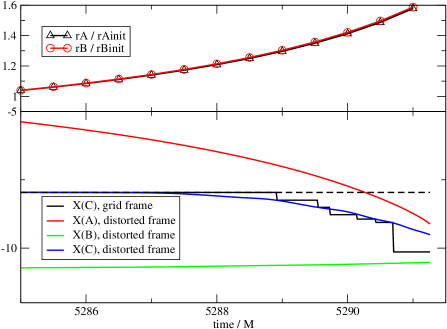
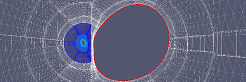
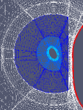
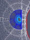
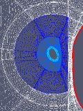
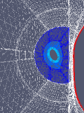
The one additional grid-boundary that needs to be dynamically controlled at plunge is the CutX plane. As seen in Fig. 13, the larger black hole tends to grow very rapidly in the distorted frame in the final few of evolution time. With its origin at a fixed location, this implies that the coordinate position of its point closest to the small black hole will rapidly approach the smaller object, with the CutX plane in the way. The dashed black line shows that if this plane were held at a fixed location, the run would have crashed at before merger. The CutX control system described in Ref. \refciteHemberger:2012jz is designed to handle this, keeping the map from the grid to the inertial frame non-singular throughout the merger. However, as stated earlier, it is essential that all individual maps in Eq. (33) are also non-singular and invertible (e.g., for the sake of the horizon finder interpolator which needs to map the position of the horizon mesh points into the grid frame). This means that the excision boundary, under the action of the shape map , must not cross the CutX plane. For this reason, at a set of discrete times, we re-position the CutX grid-plane (as shown by the black curve in Fig. 13), such that it stays between the excision boundaries (and the spherical shells surrounding these) at all times, and in all frames. Fig. 14 shows the grid-structure surrounding the two excision boundaries during such a change. Given that the subdomains are not split or joined but that their shape is redefined, we regard this algorithm as type mesh refinement.
6.4 Overall AMR performance
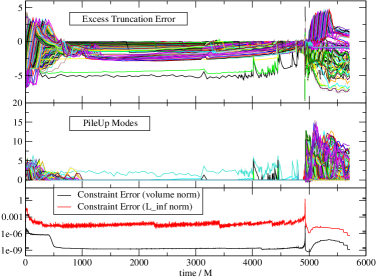
As indicated in the various sections describing our AMR algorithm, a number of aspects would benefit from improvement. Overall, however, AMR has become an essential part of our production simulations. It avoids the need to repeat the same simulation, time after time, iterating on the grid extents of the domain. Neither do we have to contend with exponential error growth, a direct consequence of exponential convergence of our numerics and the accelerated decrease of the length-scales, as dictated by the nature of the BBH inspiral and merger problem. in Fig. 15 we plot the measured truncation error level for each irreducible topology of each subdomain, the associated pile-up mode function and the overall constraint error, as measured by the global and norms. This figure shows that during the inspiral the AMR driver does quite well in keeping these quantities within control. The constraint error spike shortly before corresponds to merger. While one would prefer no such spike, we note that the spike vanishes as soon as ringdown part of our simulation begins, when the excision boundary is now based on the common horizon. This implies that the large errors are well within the newly formed black hole and do not affect the physics of the region outside the new excision boundary.
Aside from this spike, there are two other problem areas one can point to on this plot. The junk radiation has been a long-standing problem for us. Resolving it would require an unreasonable amount of computational resources for a given simulation. We are looking for alternative ways of tackling this problem. Another problem arises in the ringdown, where truncation reaches levels near and pile-up modes are created. The constraint error in this part of the run remains small, however. One possible reason why our truncation error estimate indicates large error is that the grid used to propagate the gravitational waves generated by the quasinormal modes may not be optimal once the black hole settles down. A proper -type AMR driver would possibly join the rather large number of spherical shells into a handful of subdomains once the spacetime reaches a smooth, stationary state.
Our largest concern, at the moment, is improved junk radiation treatment, as noise in the late ringdown has only a minimal effect on the primary output of our code – the gravitational waveform emitted by the BBH system.
7 Optimization
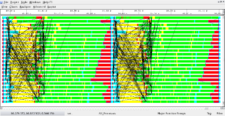
As a last element of our description we highlight one particular aspect of the optimization work that was done to SpEC. In our current parallelization scheme tasks associated with a particular subdomain are handled by a single process, with no multi-threading. Given the small number of such subdomains, the maximum number of processes one can meaningfully use in a BBH simulation is (assuming or core nodes). This on its own is a limitation we’ll possibly need to deal with by adding multi-threading to our code. But, even before that, the varying number of points per subdomain means that if each process owns a single subdomain, the work load per process would be far from even. Reducing the number of processes would help a little but, even in that case, load balancing would be very coarse grained. In order to improve this situation, we have implemented an adaptive parallel interpolation and differentiator (PID) algorithm that dynamically re-assigns as much as of the workload associated with a given subdomain from processes with too much work to those with too little. MPI_Barrier calls, issued after each RHS evaluation, are used to monitor which process is working hardest. If the cost of these MPI_Barrier calls is consistently much smaller on a particular process than on some other process, the process with the small measured MPI_Barrier cost must be busy (see Fig. 16). In this case, the process would no longer be responsible for interpolating data, as required in the inter-subdomain boundary algorithm. Neither would this process be responsible for differentiating the evolution variables. Rather, through a sequence of non-blocking MPI calls, this data would be sent to a less busy process. After all such initial messages have been sent, each process starts to compute the various pieces of the RHS (in this case: the pieces of Eq. (8) that do not involve derivatives). At various points during this RHS evaluation, the evolution algorithm dials back into the adaptive PID algorithm to see if any of the non-blocking messages have arrived at their destination. If so, data is processed (i.e., interpolated and/or differentiated). Then the processed data is sent on its way – the derivative data needs to get back to the process responsible for updating the corresponding subdomain, while the interpolated data is sent to those processes that need this data to complete the RHS evaluation on the subdomain boundary points. At some point in the RHS evaluation the derivative data or boundary data becomes a must, i.e., no more work that can be done without it. At this point blocking MPI_Wait calls are issued, enforcing the arrival of all data needed to complete the RHS. At seen on Fig. 16, most communication is in fact complete during the first half of the RHS evaluation and there is virtually no waiting for data.
This, as well as other optimization techniques, have lead to significant performance improvement of the SpEC code. As stated earlier, there is more work to be done, in particular in the area of multi-threading.
8 Conclusion
This paper gives a tour of the main building blocks of a state-of-the art binary black hole evolution code, known as the SpEC code. We start by writing out the evolution system used in our simulations, a first order symmetric hyperbolic form of the generalized harmonic formulation. We then provide a brief description of the numerical approximation used in the code. Based on these concepts, we then detail the diagnostic quantities used to monitor (and control) the accuracy of our simulations. The definitions we provide for the truncation error, the pile-up modes and the convergence factor are then used as we give an elaborate description of our spectral adaptive mesh refinement algorithm, tuned to the problem of binary black hole evolutions. As laid out in our description, our favored method of controlling truncation error is -type mesh refinement, with a target truncation error function that is tuned to use more resolution in the strong field region. In addition, we use -type mesh refinement mostly as a means of preventing grid compression as the size of the apparent horizons (and the associated excision boundaries) increases relative to the distance between the coordinate centers of the binary. Late in the plunge, for binaries with sufficiently large mass ratios, we find -type mesh refinement to be essential; as the black holes approach, the grid layout defined at the beginning of the simulation is no longer adequate. We update the grid boundaries as dictated by the dynamics of the binary black hole plunge and merger.
Fig. 15 illustrates how well our current algorithm performs during most of the inspiral. However, our algorithm does not do well at the early stage of the run where the unphysical gravitational wave content of the initial data induces high frequency ringing of the individual black holes, which in turn generates short wavelength gravitational waves which propagate through a grid that is not designed to resolve them. As a consequence of not resolving this “junk radiation”, there is a stochastic part of the truncation error whose noise produces a floor in our convergence measurements. Our attempts to control this stochastic noise source is focused on improving the initial data algorithm, e.g., by use of the ‘joint-elimination method’ described in Ref. (\refciteZhang:2013gda).
Another phase of our run where the AMR algorithm may need improvement is the ringdown stage. The reason behind this is mostly historic – this has been the easiest part of the simulation, as evolving a single black hole is simpler than evolving a binary. We plan to improve this part of our simulation but presently it is not a the major limitation in the quality of our gravitational waveforms.
Lastly, we have provided a brief description of part of the optimization that was done on the code. This is very “raw” computer science, but it is an essential part of why are we able to perform inspirals for dozens of (or, in once case, nearly two hundred) orbits.
Future work will focus on improving the accuracy of the phase of the gravitational wave during the plunge. The dominating error source in this very dynamic part of the simulation appears to be a sub-optimal structure of the inner grid at the point where nearly all spherical shells have been removed by our shell control algorithm. This results in accumulation of orbital phase error at a faster rate than during any other part of the simulation. We expect to improve this by refining our -type AMR algorithm. We also plan on exploring the use of the constraint error driven target truncation error, as this will tighten accuracy requirements when the constraints start to grow.
As yet another future project, we plan to improve our outer boundary algorithm, as we find that reflections from the outer boundary can cause unphysical effects on the binary evolution on very long time-scales (beyond orbits).
The end goal is to enable the construction of semi-analytic (or empirical) gravitational wave models and template banks by providing numerical gravitational waveforms of sufficient accuracy, length and quantity such that modeling error does not detract from the detection of gravitational waves, or the resulting physics one can discern from the observed data.
Acknowledgments
We thank Jeffrey Winicour for his useful comments on the manuscript. We thank Dan Hemberger for providing access to data produced by the head-on BBH simulation used in some of the plots. We thank Jonathan Blackman for providing access to his unequal mass inspiral simulations, as these provided data for most of the plots. We thank Saul Teukolsky, Mark Scheel, Larry Kidder, Harald Pfeiffer and Nicholas Taylor for helpful discussions while designing the AMR code. We thank Abdul Mroue, Tony Chu, Geoffrey Lovelace and Sergei Ossokine for useful feedback on the performance of our AMR algorithm in the context of thousands of BBH simulations. A significant amount of code development was done on the UCSD cluster ccom-boom.uscd.edu. The Caltech cluster zwicky.cacr.caltech.edu is an essential element of research done with SpEC. This cluster is supported by the Sherman Fairchild Foundation and by NSF award PHY-0960291. This project was supported by the Fairchild Foundation, and the NSF grants PHY-1068881 and AST-1333520.
References
- [1] H. Friedrich, “On the hyperbolicity of Einstein’s and other gauge field equations,” Commun. Math. Phys., vol. 100, no. 4, pp. 525–543, 1985.
- [2] H. Friedrich, “On the nonlinearity of the subsidiary systems,” Class. Quantum Grav., vol. 22, p. L77, 2005.
- [3] O. Brodbeck, S. Frittelli, P. Hübner, and O. A. Reula, “Einstein’s equations with asymptotically stable constraint propagation,” J. Math. Phys., vol. 40, no. 2, pp. 909–923, 1999.
- [4] C. Gundlach, J. M. Martin-Garcia, G. Calabrese, and I. Hinder, “Constraint damping in the Z4 formulation and harmonic gauge,” Class. Quantum Grav., vol. 22, pp. 3767–3774, 2005.
- [5] F. Pretorius, “Evolution of binary black hole spacetimes,” Phys. Rev. Lett., vol. 95, p. 121101, 2005.
- [6] M. C. Babiuc, B. Szilágyi, and J. Winicour, “Testing numerical evolution with the shifted gauge wave,” Class. Quantum Grav., vol. 23, pp. S319–S342, 2006.
- [7] L. Lindblom and B. Szilágyi, “An improved gauge driver for the GH Einstein system,” Phys. Rev. D, vol. 80, p. 084019, 2009.
- [8] B. Szilágyi, L. Lindblom, and M. A. Scheel, “Simulations of Binary Black Hole Mergers Using Spectral Methods,” Phys. Rev. D, vol. 80, p. 124010, 2009.
- [9] L. Lindblom, M. A. Scheel, L. E. Kidder, R. Owen, and O. Rinne, “A new generalized harmonic evolution system,” Class. Quantum Grav., vol. 23, pp. S447–S462, 2006.
- [10] N. W. Taylor, L. E. Kidder, and S. A. Teukolsky, “Spectral methods for the wave equation in second-order form,” Phys. Rev., vol. D82, p. 024037, 2010.
- [11] H.-O. Kreiss and J. Winicour, “Problems which are well posed in a generalized sense with applications to the Einstein equations,” Class. Quantum Grav., vol. 16, pp. S405–S420, 2006.
- [12] M. Babiuc, H.-O. Kreiss, and J. Winicour, “Constraint-preserving Sommerfeld conditions for the harmonic Einstein equations,” Phys.Rev., vol. D75, p. 044002, 2007.
- [13] H.-O. Kreiss and J. Winicour, “Geometric Boundary Data for the Gravitational Field,” Class.Quant.Grav., vol. 31, p. 065004, 2014.
- [14] O. Rinne, “Stable radiation-controlling boundary conditions for the generalized harmonic Einstein equations,” Class.Quant.Grav., vol. 23, pp. 6275–6300, 2006.
- [15] B. Szilágyi, D. Pollney, L. Rezzolla, J. Thornburg, and J. Winicour, “An explicit harmonic code for black-hole evolution using excision,” Class. Quantum Grav., vol. 24, pp. S275–S293, 2007.
- [16] M. Campanelli, C. Lousto, P. Marronetti, and Y. Zlochower, “Accurate evolutions of orbiting black-hole binaries without excision,” Phys. Rev. Lett., vol. 96, p. 111101, 2006.
- [17] J. G. Baker, J. Centrella, D.-I. Choi, M. Koppitz, and J. van Meter, “Gravitational wave extraction from an inspiraling configuration of merging black holes,” Phys. Rev. Lett., vol. 96, p. 111102, 2006.
- [18] L. T. Buchman, H. P. Pfeiffer, M. A. Scheel, and B. Szilágyi, “Simulations of unequal mass binary black holes with spectral methods,” Phys. Rev. D, vol. 86, p. 084033, 2012.
- [19] A. H. Mroue, M. A. Scheel, B. Szilagyi, H. P. Pfeiffer, M. Boyle, et al., “A catalog of 174 binary black-hole simulations for gravitational-wave astronomy,” Phys.Rev.Lett., vol. 111, p. 241104, 2013.
- [20] D. A. Hemberger, M. A. Scheel, L. E. Kidder, B. Szilagyi, G. Lovelace, et al., “Dynamical Excision Boundaries in Spectral Evolutions of Binary Black Hole Spacetimes,” Class.Quant.Grav., vol. 30, p. 115001, 2013.
- [21] M. A. Scheel, H. P. Pfeiffer, L. Lindblom, L. E. Kidder, O. Rinne, and S. A. Teukolsky, “Solving Einstein’s equations with dual coordinate frames,” Phys. Rev. D, vol. 74, p. 104006, 2006.
- [22] D. Gottlieb and J. S. Hesthaven, “Spectral methods for hyperbolic problems,” J. Comput. Appl. Math., vol. 128, no. 1–2, pp. 83–131, 2001.
- [23] J. Hesthaven, S. Gottlieb, and D. Gottlieb, Spectral Methods for Time-Dependent Problems. Cambridge, UK: Cambridge University Press, 2007.
- [24] M. J. Berger and J. Oliger, “Adaptive mesh refinement for hyperbolic partial differential equations,” J. Comput. Phys., vol. 53, pp. 484–512, 1984.
- [25] F. Zhang and B. Szilágyi, “A joint approach for reducing eccentricity and spurious gravitational radiation in binary black hole initial data construction,” Phys.Rev., vol. D88, p. 084033, 2013.