Quantum phase transition in one-dimensional commensurate Frenkel-Kontorova model

Abstract

In this paper, we have studied the one-dimensional commensurate quantum Frenkel-Kontorova model by a density-matrix renormalization group (DMRG) algorithm. The focus has been on its properties of the entanglement, the coordinate correlation, the ground state energy and the energy gap between the ground state and the first excited one. It is demonstrated that a quantum phase transition (QPT) between the pinned and the sliding phases takes place as the quantum fluctuation, measured by an effective Planck constant $\tilde{\hbar}$, increases to a threshold value $\tilde{\hbar}_{c}$.

1 Introduction

The Frenkel-Kontorova model (FK model) [1, 2, 3] describes a chain of interacted particles in the presence of an external periodic potential which has attracted much attention ever since it first appeared in last century [4]. In the continuum approximation, the model will be reduced to the well-known integrable sine-Gordon equation. But as a discrete model, it is nonintegrable and has been a generic tool to study many nonlinear effect such as chaos, kinks, breathers and so on [4, 5, 6, 7]. In condense matter physics, it also has a wide range of application, such as describing an adsorbate layer on the surface of a crystal [8], charge-density-wave transport [9], dry friction [10] and a chain of coupled Josephson junctions [11].

Many of the interesting properties of the classical FK model come from its two competing length scales: the average distance between the particles and the length of the spacial period of the external potential. For example, if the ratio of the two scales is a rational number, the system is commensurate, otherwise, it is incommensurate. For the former case, a classical FK model is always in a pinned state. For the latter case, there is a threshold $K_{c}$. If $K>K_{c}$, the particles are still pinned. But if $K<K_{c}$, the particles are depinned, and can slide along the external potential.

No matter whether the classical is commensurate or incommensurate, intuitively, all the pinned state can transit to a sliding one so long as enough quantum fluctuations are introduced. Up to now, there have been a lot of discussions upon this quantum phase transition (QPT) for the incommensurate case [12, 13, 14, 15]. But as far as QPT is concerned, the commensurate case is also a very interesting topic to discuss since it is a physically more clean case and we will be save from all those classical complexities specific to incommensurate FK model any more.

Unlike the classical phase transition during which temperature plays a major role, QPT occurs as a result of the quantum fluctuations. In condensed matter physics, QPT is a very hot subject due to its close connection to some fundamental problems such as quantum criticality and high-temperature superconductivity [16]. Usually, the QPT is driven by changing some nonthermal external parameters. But for the QPT we are going to study in this paper, it is induced directly by the quantum fluctuation just like we change the temperature in classical phase transition. It is hoped that this different angle can provide some new perspective to QPT since the physical detail of the QPT process is still far from being well understood.

In the article, we will try to use the entanglement, the coordinate correlation, the ground state energy and the energy gap between the ground state and the first excited state to find the transition point.

To solve the quantum FK model, the density matrix renormalization group (DMRG) method will be used, which is developed more than two decades ago by White[17]. It is well known for the high-accuracyin simulating the low-dimensional strongly correlated quantum systems [18]. The scheme of standard DMRG algorithm can be found in many reference [19, 17, 20, 18] and the concrete realization in FK model has been given in Refs. [21]. So the the detail will not be presented here. We will just briefly review the FK model to introduce the necessary notations in the next section.

2 Quantum FK Model

Figure 1: Schematic diagram of the Frenkel-Kontorova model. A chain of $N+2$ particles connect by springs is subjected to the action of external sinusoidal potential with spacial period $b$. The average distance between neighboring particles is $a=L/(N+1)$.

Fig. 1 presents the schematic diagram of the one-dimensional Frenkel-Kontorova model [4]: a chain of $N+2$ particles connected by springs and subjected to the action of an external sinusoidal potential. The average distance between neighboring particles and the external potential period are $a=L/(N+1)$ and $b$, respectively, where $L$ is the length of the chain. For the commensurate case we are interesting in this paper, $a/b$ is set to be $1$. By using the fixed boundary conditions with $x_{0}=0,x_{N+1}=(N+1)a$, the Hamiltonian can be expressed as,

$$\hat{H}=\sum_{i=1}^{N}[-\frac{\hbar^{2}}{2m}\frac{\partial^{2}}{\partial x_{i}^{2}}+\frac{k}{2}(\hat{x}_{i+1}-\hat{x}_{i}-a)^{2}-V\cos(\frac{2\pi}{b}\hat{x}_{i})],$$ (1)

where $\hbar$ is the Planck, $k$ is the elastic constant and $V$ is the potential amplitude.

With $q_{0}=2\pi/b$ , we introduce the dimensionless parameters,

$$\hat{X}_{i}=q_{0}{\hat{x}_{i}},\quad\hat{U}_{i}=\hat{X}_{i}-i\cdot 2\pi,\quad\hat{H^{\prime}}=\frac{q_{0}^{2}}{k}\hat{H},$$

$$K=V\frac{q_{0}^{2}}{k},\quad\tilde{\hbar}=\frac{q_{0}^{2}}{\sqrt{mk}}\hbar.$$ (2)

Then the Hamiltonian can be rewritten in a dimensionless form,

$$\hat{H^{\prime}}=\sum_{i=1}^{N}[-\frac{\tilde{\hbar}^{2}}{2}\frac{\partial^{2}}{\partial U_{i}^{2}}+\frac{1}{2}({\hat{U}_{i+1}}-{\hat{U}_{i}})^{2}-K\cos(\hat{U_{i}}+i\cdot 2\pi)].$$ (3)

By using the following transformations,

$$\hat{U_{i}}=\frac{1}{\sqrt{2}}\frac{\sqrt{\tilde{\hbar}}}{\sqrt[4]{2}}({\hat{a}_{i}}^{{\dagger}}+{\hat{a}_{i}}),$$

$$\hat{P_{i}}=\frac{\partial}{\partial{U_{i}}}=-\frac{1}{\sqrt{2}}\frac{\sqrt[4]{2}}{\sqrt{\tilde{\hbar}}}({\hat{a}_{i}}^{{\dagger}}-{\hat{a}_{i}}),$$ (4)

where $\hat{a}_{i}^{{\dagger}}$ and $\hat{a}_{i}$ are the annihilation and creation operators satisfying $[\hat{a}_{i},\hat{a}_{j}^{{\dagger}}]=\delta_{ij}$, $[\hat{a}_{i},\hat{a}_{j}]=0$, $[\hat{a}_{i}^{{\dagger}},\hat{a}_{j}^{{\dagger}}]=0$, we can rewrite the Eq. (3) into a second-quantized form,

$$\hat{H^{\prime}} = \sqrt{2}\tilde{\hbar}\sum_{i=1}^{N}\{({\hat{a}_{i}}^{{\dagger}}{\hat{a}_{i}}+\frac{1}{2})$$ (5)

$$-\sqrt{2}\tilde{\hbar}\sum_{i=1}^{N}(\hat{a}_{i}^{{\dagger}}+\hat{a}_{i})(\hat{a}_{i+1}^{{\dagger}}+\hat{a}_{i+1})$$

$$-\frac{K}{\sqrt{2}\tilde{\hbar}}\cos[\frac{1}{\sqrt{2}}\frac{\sqrt{\tilde{\hbar}}}{\sqrt[4]{2}}(\hat{a}_{i}^{{\dagger}}+\hat{a}_{i})+i\cdot 2\pi]\}.$$

From the above equation, it is easy to see that there are two independent parameters: $\tilde{\hbar}$ and $K$. The first is the effective Plank constant, denoting the quantum fluctuation. The second measures the strength of external potential. These two free effective parameters can be varied by changing the elastic constant $k$, the particle mass $m$, the spacial period $b$ or the magnitude of the external potential $V$ according to Eq. (2).

3 RESULTS AND DISCUSSIONS

In the incommensurate case, some dumb particles (or glue particles) have been found in FK model, which are located very close to the bottoms of the potential, dividing the whole chain into several subblocks (bricks) [22]. The particles inside the subblocks can interact each easily and remains unaffected by the outside particles. As the quantum fluctuation increases, the dumb particles will change into normal ones and the bricks melt, thus a new sliding phase appears and the QPT occurs. In the commensurate case, the same scenario can be realized since every particle will look like a dumb particle. Then as the quantum fluctuation is introduced, QPT will happens.

3.1 Entanglement

(a)

(b)

Figure 2: (a)The variation of entanglement $S_{E}$ against the effective Planck constant $\tilde{\hbar}$ for different system size with $K=5$. (b) The same as in (a) but for the first-order derivative of $S_{E}$.

As a complex quantum phenomenon, the entanglement is famous for its possible utilization as a resource in quantum communications and computations [23]. Recent work has shown that entanglement can also be used as an order parameter to study QPT in condensed matter physics. For example, it has been demonstrated that for many one-dimensional magnetic systems, the entanglement shows scaling behaviour in the vicinity of the transition point [24]. For the moment, a lot of work have been done upon the relation between the entanglement and QPT [25, 26, 27, 29, 30, 28]. Hence we have a good reason to check the entanglement in our work.

The von Neumann entropy will be used to measure the entanglement [31], which is defined as,

$$S=-tr(\rho\log\rho),$$ (6)

where $\rho$ is the density matrix of the state we are interested in and $tr$ denotes the trace In our work, the following average entanglement between a single particle and the rest of the systems is calculated,

$$S_{E}=\frac{1}{n}\sum\limits_{i=1}^{n}S_{i},$$ (7)

in which $S_{i}=-tr_{i}(\rho_{i}\log\rho_{i})$ is the von Neumann entropy corresponding to $i$th site with $\rho_{i}=Tr_{i}\left|\Psi\right\rangle\left\langle\Psi\right|$[25, 26, 27]. Here $Tr_{i}$ stands for the tracing over all sites except the $i$th site.

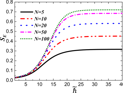
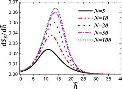
Fig. 2(a) gives the variation of $S_{E}$ against $\tilde{\hbar}$ for different system size with fixed external potential $K=5$. It is easy to see that $S_{E}$ increases with $\tilde{\hbar}$ until it reaches the maximum. Moreover, for bigger system size, $S_{E}$ increases faster with $\tilde{\hbar}$, but reaches the maximum value more slowly. This implicates that although the smaller system has lower maximum entanglement, as a whole it can be entangled much easier when the quantum fluctuation is introduced. In other words, we need higher quantum fluctuations to entangle the bigger system. This is consistent with our physical intuitive. As the system size become bigger and bigger, it is important to note that the curves tend to converge to one curve. To see the significance of this effect, we plot the first-order derivative of $S_{E}$ in Fig. 2(b). One marvelous observation is that there is a peak for each curve. And the position of the peak approaches a definite value of $\tilde{\hbar}_{c}\approx 13$ as the system size is increased. From the recent research upon the entanglement and QPT [28], we can regard $\tilde{\hbar}_{c}$ here as a phase transition point from pinned state to a sliding one. Compared with the transition point at $\tilde{\hbar}_{c}\approx 2$ for the incommensurate quantum FK model with the same external potential [21, 12], $\tilde{\hbar}_{c}\approx 13$ is a much higher value. This difference can be attributed to their classical behaviours. For example, the incommensurate FK system can only get pinned when $K$ is bigger than $1$, which is called Transition by Breaking Analyticity (TBA) in classical physics [8]. But the commensurate FK system will get pinned for any slight of external potential.

(a)

(b)

Figure 3: Contour map demonstrating the dependence of $S_{E}$ in (a) and $\frac{dS_{E}}{d\tilde{\hbar}}$ in (b) upon $\tilde{\hbar}$ and $K$, respectively. $N=50$. The skeleton of maximum points give the phase transition line(the black line in(b)).

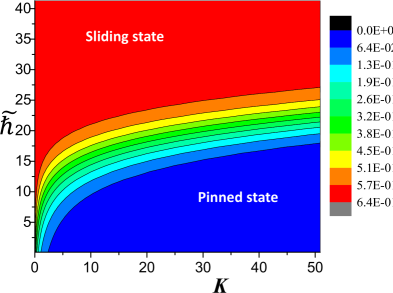
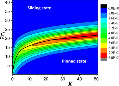
For different external potential, the transition point of $\tilde{\hbar}_{c}$ will change. In Fig. 3(a), we presents the contour map of $S_{E}$ in the $K-\tilde{\hbar}$ parameter space. Although $S_{E}$ is a complicated function of both $K$ and $\tilde{\hbar}$, we can still see two obvious phases. The pinned phase is in the region where $K$ is large or $\tilde{\hbar}$ is small. The sliding phase is in the region where $K$ is small or $\tilde{\hbar}$ is large. There exists a transition zone between the two phases, which illustrates how the transition happens. In order to find out the transition points, we also give the contour map of $\frac{dS_{E}}{d\tilde{\hbar}}$ on the $\tilde{\hbar}-K$ plane in Fig. 3(b). The transition curve can be obtained by tracing the points of the maximum $\frac{dS_{E}}{d\tilde{\hbar}}$ for each definite $K$ in the direction of $\tilde{\hbar}$ axis or just roughly by following the tips of the contour lines. For example, when $K=5$, $\tilde{\hbar}_{c}\approx 13$ can be acquired, which is consistent with the result given by Fig. 2(b).

3.2 Coordinate correlation

(a)

(b)

Figure 4: (a) Variation of the correlation of different lengthes denoted by $L$ against the quantum fluctuation. The system size is set to $N=50$ and external potential $K=5$. (b) The same as in (a) but for the first-order derivative of $S_{E}$ with respect to $\tilde{\hbar}$.

Besides the entanglement, there is also other kind of quantum correlations. In this section, we will discuss the coordinate correlation, which is written as

$$\tilde{\hbar}G_{ij}=<\Psi_{0}\mid(X_{i}-\bar{X}_{i})(X_{j}-\bar{X}_{j})\mid\Psi_{0}>,$$ (8)

from which we can define the correlation of length $L$,

$$C^{L}=\tilde{\hbar}G_{ij}\delta(\left|i-j\right|-L).$$ (9)

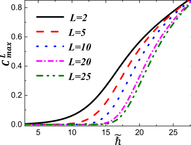
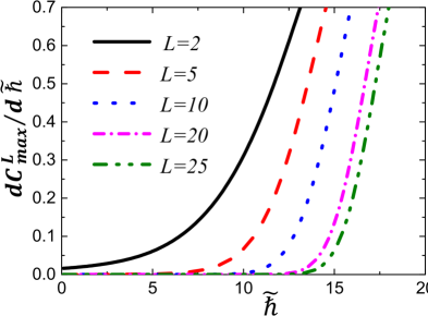
For $i,j$ satisfying $i-j=L$, the maximum value of $C^{L}$ will be used to embody the coordinate correlation of length $L$, denoted as $C^{L}_{max}$. Fig. 4(a) gives the relationship between $C^{L}_{max}$ and $\tilde{\hbar}$ for different correlation length $L$. For comparison, $C^{L}_{max}$ has been normalized [0,1] for each curve and the system size is chosen to be $50$. It is interesting to see that as the quantum fluctuation begins to set in, the correlation between the particles with distance $L=2$ emerges first and increases with $\tilde{\hbar}$. Then correlation with longer length $L$ begins to appear when $\tilde{\hbar}$ is increased further. Finally, around $\tilde{\hbar}_{c}\approx 13$, the correlation of length $L=25$, which is about half of system size $N=50$, starts to dominate the system. This is also the transition point corresponding to the entanglement that changes most rapidly with the quantum fluctuation. Like entanglement, we have also studied the changing speed of $C^{L}_{max}$ with $\tilde{\hbar}$, i.e. $\frac{dC^{L}_{max}}{d\tilde{\hbar}}$ , which is presented in Fig. 4(b), where each curve is normalized to (0,1) just as in Fig. 4(a). The same point at $\tilde{\hbar}_{c}\approx 13$ can be found to correspond to the maximum increasing speed of the correlation with length $L=25$.

Figure 5: The entanglement $C$ against the effective Planck constant $\tilde{\hbar}$ for a FK-chain with $N=50$ and $K=5$.

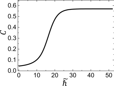
In order to find out the relationship between the correlations and QPT, we introduce the following parameter,

$$C=\frac{\sum_{L=1}^{N}C^{L}_{FKmodel}}{~{}\sum_{L=1}^{N}C^{L}_{Harmomic}},$$ (10)

where $C^{L}_{FKmodel}$ and $C^{L}_{Harmomic}$ denote the $C^{L}$ of the FK model and the oscillator chain respectively. The results are given in Fig. 5, from which we can observe an obvious change of the correlations around $\tilde{\hbar}_{c}\sim 13$. It is not a sharp change, which may result from the finite-size effect.

3.3 Ground state energy and energy gap

For the ground state of a classical commensurate FK chain, the particles are localized by the external potential. As the quantum effect comes in, they will gain kinetic energy due to the quantum fluctuations. As the gained kinetic energy is high enough to help the particles overcoming the trapping potential, the whole system can be expected to get depinned and become a sliding state.

Figure 6: (a) The variation of the ground state energy against the quantum fluctuation denoted by $\tilde{\hbar}$. For contrast, the results for a chain of harmonic oscillators are also presented. (b) gives the dependence of the energy gap $\Delta E_{12}$ and with respect to $\tilde{\hbar}$. The other parameters in the calculations are $N=100$ and $K=5$.

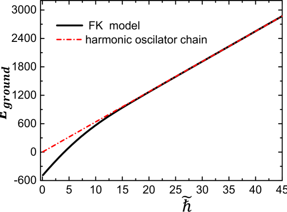
Fig. 6 gives the dependence of the ground state energy $E_{ground}$ upon $\tilde{\hbar}$. For contrast, the corresponding curve for a harmonic oscillator chain is also given. The chain size is set to be $N=50$ for both systems and the external potential for the FK model is $K=5$. It is apparent $E_{ground}$ increases with $\tilde{\hbar}$. Moreover the difference of the ground state energy between the FK model and the harmonic oscillator chain gets smaller and smaller until the two curves almost overlap with each other at about $\tilde{\hbar}_{c}\approx 13$, which implicates a phase transition from the pinned state to the sliding one. This phenomenon also tells us that the behaviour of the sliding state is more like a harmonic oscillator chain with the accretion of quantum fluctuations.

Figure 7: The variation of the energy gap $\frac{\Delta E_{12}}{\tilde{\hbar}}$ against the quantum fluctuation denoted by $\tilde{\hbar}$ for different system size. The parameters is $K=5$.

Figure 8: The energy gap $\frac{\Delta E_{12}}{\tilde{\hbar}}$ and its first and second order derivatives of a FK chain. The parameters are $N=100$ and $K=5$.

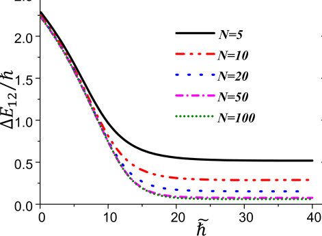
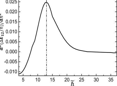
Fig. 7 presents the result of the energy gap $\Delta E_{12}$ between the ground state and the first excited state for different system sizes. Because the energy gap for the harmonic oscillator chain, $\Delta E_{12}=\tilde{\hbar}\cdot\sin\frac{\pi}{2(N+1)}$, shows a linear dependence upon $\tilde{\hbar}$, we have scaled the ordinate axis by $\tilde{\hbar}$ in Fig. 7 so that $\Delta E_{12}/\tilde{\hbar}$ will become a constant in this ideal model. It is interesting to note that when $\tilde{\hbar}$ is big enough, $\Delta E_{12}/\tilde{\hbar}$ in FK model also becomes a constant just like the harmonic oscillator chain. This result is consistent with the conclusion from the above study upon the ground state energy. To get the transition point, we plot the second derivative of $\Delta E_{12}/\tilde{\hbar}$ with respect to $\tilde{\hbar}$ for the size $N=100$. Here again we find the characteristic value $\tilde{\hbar}_{c}\approx 13$, at which $\Delta E_{12}/\tilde{\hbar}$ shows a peak. So by summarizing all the data we have obtained until now, the phase transition point can be consitently set to be $\tilde{\hbar}_{c}\approx 13$.

4 SUMMARY

In summary, we have investigated in details the phase transition from the pinned state to the slidingone in the one-dimensional commensurate quantum FK model with a density-matrix renormalization group algorithm. By looking into the entanglement, the particle coordinate correlation, the ground state energy and the energy gap, a transition point with $\tilde{\hbar}_{c}\approx 13$ is found when the external potential is set to be $K=5$. In the sliding state, the system behaves much like a chain of harmonic oscillators. It is hoped that the research work in this paper will not only help us to understand more the quantum FK model in describing many condensed matter systems, but also find applications in quantum information processing (QIP), such as the cold trapped ions in an optical lattice, which has been put forward as a new realization of quantum FK model recently [32].

This work is supported by the National Natural Science Foundation of China under Grant Nos. 11274117 and 11134003 and Shanghai Excellent academic leaders Program of China (Grant No. 12XD1402400).

References

- [1] Frenkel Ya and Kontorova T 1938 Phys. Z. Sowietunion 13, 1
- [2] Kontorova T A, Frenkel Ya I 1938 Zh. Eksp. Teor. Fiz 8, 89
- [3] Kontorova T A, Frenkel Ya I 1938 Zh. Eksp. Teor. Fiz 8, 1340
- [4] Braun M and Kivshar Y S, 2003 The Frenkel-Kontorova Model: Concepts, Methods, and Applications (Springer, Berlin)
- [5] Chirikov B V 1979 Phys. Rep. 52, 263
- [6] Consoli L, Knops H J F and Fasolino A 2000 Phys. Rev. Lett. 85, 302
- [7] Ying S C 1971 Phys. Rev. B, 3, 4160
- [8] Aubry S 1978 in Solitons and Condensed Matter Physics, edited by A. R. Bishop and T. Schneider (Springer,New York).
- [9] Floria L M and Mazo J J 1996 Adv. Phys. 45, 505
- [10] Braun O M, Dauxois T, Paliy M V and Peyrard M,1997 Phys. Rev. Lett. 78, 1295
- [11] Watanabe S, van der Zant H S J , Strogatz S H and Orlando T P 1996 Physica D 97, 429
- [12] Zhirov O V, Casati G and Shepelyansky D L 2003 Phys. Rev. E 67, 056209
- [13] Zhirov O V, Casati G and Shepelyansky D L 2002 Phys. Rev. E 65, 026220
- [14] Schilling R 1984 Phys. Rev. Lett. 53, 2258
- [15] Reichert P 1985 Schilling R, Phys. Rev. B 32, 5731
- [16] Sachdev S and Keimer B 2011 Phys. Today 64, 29
- [17] White S R 1992 Phys. Rev. Lett. 69, 2863
- [18] White S R and Feiguin A E 2004 Phys. Rev. Lett. 93, 076401
- [19] Caron L G and Moukouri S 1997 Phys. Rev. B. 56, 8471
- [20] White S R 1993 Phys.Rev. B 48, 10345
- [21] Hu B and Wang J 2006 Phys. Rev. B 73, 184305
- [22] Zhirov O V, Casati G and Shepelyansky D L 2005 arXiv:cond-mat/0501188 [cond-mat.dis-nn]
- [23] Kais S, 2007 In Adv. Chem. Phys. Edited by D.A. Mazziotti(Wiley, New York) 134, P. 493
- [24] Osterloh A, Amico L, Falci G and Fazio R,2002 Nature 416, 608
- [25] O Connor K M and Wootters W K 2001 Phys. Rev. A 63, 052302
- [26] Wang X 2001 Phys. Rev. A 64, 012313.
- [27] Kamta G L and Starace A F 2002 Phys. Rev. Lett. 88, 107901
- [28] Gu S J, Deng S S, Li Y Q and Lin H Q 2004 Phys. Rev. Lett. 93, 086402
- [29] Vidal G, Latorre J I, Rico E and Kitaev A 2003 Phys. Rev. Lett. 90, 227902
- [30] Latorre J I, Rico E and Vidal G 2004 Quant. Inf. Comp. 4, 48
- [31] Bennett C H, Bernstein H J, Popescu S and Schumacher B 1996 Phys. Rev. A 53, 2046
- [32] Garcia-Mata I, Zhirov O V, and Shepelyansky D L 2007 Euro. Phys. J. D 41, 325