Coil-helix transition of polypeptide at water-lipid interface

Abstract

We present the exact solution of a microscopic statistical mechanical model for the transformation of a long polypeptide between an unstructured coil conformation and an $\alpha$-helix conformation. The polypeptide is assumed to be adsorbed to the interface between a polar and a non-polar environment such as realized by water and the lipid bilayer of a membrane. The interfacial coil-helix transformation is the first stage in the folding process of helical membrane proteins. Depending on the values of model parameters, the conformation changes as a crossover, a discontinuous transition, or a continuous transition with helicity in the role of order parameter. Our model is constructed as a system of statistically interacting quasiparticles that are activated from the helix pseudo-vacuum. The particles represent links between adjacent residues in coil conformation that form a self-avoiding random walk in two dimensions. Explicit results are presented for helicity, entropy, heat capacity, and the average numbers and sizes of both coil and helix segments.

1 Introduction

The folding mechanisms of water-soluble proteins from primary to secondary and higher-order structures has been thoroughly investigated over many years. In the study of protein translocation pathways into and across cell membranes, which is a very important active area of current research, one important problem requiring further elucidation is the coil-helix transition that accompanies the insertion of a polypeptide into a lipid bilayer. The theoretical modeling of this ubiquitous process in biological matter is fairly complex due to the heterogeneous environment in which conformational changes occur and the simultaneity or rapid succession of conformational change and translocation. Experimental studies are limited to the small selection of polypeptides that are water soluble and undergo controllable insertion/folding and exit/unfolding processes.

The folding of all helical membrane proteins/peptides, independent of the insertion mechanism, is governed by the formation of helical segments in the lipid bilayer environment. This process is driven by hydrophobic interactions and hydrogen bonding [1, 2, 3, 4]. Its two main steps are the transformation from coil to interfacial helix and the insertion of the helix into the membrane with transmembrane orientation. Variants of the pH Low Insertion Peptide (pHLIP) family are water soluble and prove to be well suited for the investigation of membrane-associated folding and unfolding [5, 6], reversibly driven by changes in pH. A drop in pH leads to the protonation of negatively charged side chains, which enhances the hydrophobicity of the peptide and initiates the aforementioned two-step process of folding and insertion. A subsequent rise in pH reverses the process: the peptide unfolds and exits. Recent experimental studies have already established important thermodynamic and kinetic parameters of the peptide-membrane interaction [7, 8, 9].

What has been lacking for these and related experiments is a microscopic statistical mechanical model with experimentally testable attributes that is amenable to an exact analysis. Our goal is to construct, solve, develop, and test such a model in three successive stages. The first stage, which is theme of this paper, involves the design and solution of a microscopic model that describes the coil-helix transformation of a long polypeptide adsorbed to the lipid bilayer of a membrane membrane (see Fig. 1).

Figure 1: (Color online) Long polypeptide at the interface between water and a flat lipid bilayer undergoing a reversible and pH-driven coil -helix transformation.

Such a model is an indispensable part of a theory of membrane-associated folding and will be used as the foundation for the next two stages. They include (a) the investigation of profiles of local attributes for generic polypeptides and landscapes of global attributes for short peptides such as pHLIP in the heterogeneous water/lipid environment and (b) the kinetics of insertion and exit as can be inferred from the landscapes of free energy and conformational attributes.

The pioneering theoretical studies of coil-helix transformations and related phenomena that appeared throughout 1960s were admirably compiled and reviewed in a monograph by Poland and Scheraga [10]. A series of model systems were introduced at that time. Many of them are still being used today in textbooks and research papers. This includes the familiar Zimm-Bragg model [11] and generalizations thereof, all amenable to the transfer matrix method of analysis. Also emerging at that time was the highly original Lifson method of statistical mechanical analysis [12], the scope of which includes (smooth) crossovers and (sharp) transitions [13, 14]. The need at this time for yet another model solved by yet a different method is dictated by the three stages of our project as will become apparent in what follows.

In Sec. 2 we present the microscopic model of our design as a system of statistically interacting links and describe the method of its exact analysis. Depending on the parameter settings the exact solution produces a conformational change in the form of a crossover or a transition (Sec. 3). The transition may be of first or second order as we discuss in Sec. 4 with focus on the helicity (order parameter) and entropy (measure of disorder) and other quantities. In Sec. 5 we summarize the main advances of this work and point out their role as the foundation for the continuation of this project in two different directions in the arenas of biological physics and statistical mechanics. We also discuss how this work connects to recent studies by other researchers and how the continuation of this project can benefit from those studies.

2 Model system

The microscopic model that we present here is a system of statistically interacting quasiparticles with shapes. The methodology employed for its exact statistical mechanical analysis is built on the concept of fractional statistics, invented by Haldane [15], and developed by Wu [16], Isakov [17], Anghel [18], and others [19] in the context of quantum many-body systems. The adaptation of this approach to classical statistical mechanical systems of particles with shapes was developed in a recent series of studies with applications to Ising spins [20, 21, 22, 23], jammed granular matter [24, 25], lattice gases with long-range interactions [26], and DNA under tension [27]. The application to the coil-helix transition of a long polypeptide adsorbed to a water-lipid interface worked out in the following is conceptually simple but surprisingly rich in scope.

2.1 Coil segments from helix vacuum

The reference state (pseudo-vacuum) of our model system is the ordered helix conformation of $N$ residues bound by peptide bonds into $N-1$ links and stabilized by internal hydrogen bonds along the backbone. Thermal fluctuations or environmental change cause the nucleation of disordered coil segments, which then grow by unravelling adjacent helical order.

In our model the coil segments are represented by thermally activated links that combine to form a self-avoiding random walk between the ends of successive helical segments. Both coil and helix segments are confined to the water-lipid interface (Fig. 1). Coil segments carry configurational entropy that grows with their size and range in the interfacial plane. That range is controllable at a microscopic level by the integer-valued model parameter $\mu$, henceforth called range parameter.

Each residue can be in $\mu+1$ states, of which one (denoted h) represents the helix conformation and $\mu$ (numbered 1, …, $\mu$) represent the coil conformation. Access by a residue to these states is constrained by the states of its neighboring residues as illustrated in Fig. 2 for the case $\mu=3$.

Figure 2: Segment of coil conformation between two segments of helix conformation (bottom), generated by the activation of $2\mu$ species of statistically interacting particles in the form of single links or composed of pairs of links that are not necessarily adjacent (top). Residues in helix conformation are in a unique state (h). Residues in coil conformation are in one of $\mu$ states $(1,2,...,\mu)$, constrained to to form a self-avoiding walk in the interfacial plane and here illustrated for $\mu=3$.

Helical links (hh) are short and form straight segments (horizontal, in Fig. 2) in the plane of the water-lipid interface. Coil links are more extended and directed either horizontally (11, 22, 33) or vertically (h1, 12, 23, 32, 21, 1h). Our model allows each coil segment to randomly explore the interface on one side of the helical direction without intersecting itself. That space is discretized and constrained by the length of the segment and by the number of distinct coil states.

We assign different activation energies to coil links relative to hh links depending on whether they contribute to nucleation or to growth. To the former we assign the activation energy $\epsilon_{\mathrm{n}}$ and to the latter $\epsilon_{\mathrm{g}}$ (two model parameters). Nucleation of one coil link requires the simultaneous break-up of several internal hydrogen bonds whereas growth proceeds by the break-up of one bond per link (two bonds shared by different pairs of residues). On our way to calculating a partition function we now face the task of counting microstates of given link content.

2.2 Combinatorics of links

For the combinatorial analysis we introduce a set of statistically interacting quasiparticles that contain individual links or pairs of links. It turns out that we need $2\mu$ species of particles. In the case of $\mu=3$ they are the six species (along with the element of pseudo-vacuum) shown in the top panel of Fig. 2. The combinatorics of statistically interacting particles is captured by the energy expression

$$E(\{N_{m}\})=E_{\mathrm{pv}}+\sum_{m=1}^{2\mu}N_{m}\epsilon_{m},$$ (1)

and the multiplicity expression [15, 16, 17, 18, 19, 20, 21],

$$W(\{N_{m}\})=\prod_{m=1}^{2\mu}\left(\begin{array}[]{cc}d_{m}+N_{m}-1\\ N_{m}\end{array}\right),$$ (4)

$$d_{m}=A_{m}-\sum_{m^{\prime}=1}^{2\mu}g_{mm^{\prime}}(N_{m^{\prime}}-\delta_{mm^{\prime}}),$$ (5)

inferred from a generalized Pauli principle as will be illustrated below for the application under consideration. This means that there exist $W(\{N_{m}\})$ microstates with energy $E(\{N_{m}\})$ that all have the same particle content: $N_{m}$ particles of species $m$ for $m=1,\ldots,2\mu$. The $\epsilon_{m}$ are particle activation energies relative to the energy $E_{\mathrm{pv}}$ of the pseudo-vacuum, the $A_{m}$ are capacity constants, and the $g_{mm^{\prime}}$ are statistical interaction coefficients. The specifications for the model with $\mu=3$ distinct coil states are compiled in Table 1.

Table 1: Specifications of the six species of particles that describe the case $\mu=3$.

motif	cat.	$m$	$\epsilon_{m}$	$A_{m}$
$\mathsf{h1h}$	host	$1$	$\epsilon_{\mathrm{n}}$	$N-2$
$\mathsf{121}$	hybrid	$2$	$2\epsilon_{\mathrm{g}}$	$0$
$\mathsf{232}$	hybrid	$3$	$2\epsilon_{\mathrm{g}}$	$0$
$\mathsf{11}$	tag	$4$	$\epsilon_{\mathrm{g}}$	$0$
$\mathsf{22}$	tag	$5$	$\epsilon_{\mathrm{g}}$	$0$
$\mathsf{33}$	tag	$6$	$\epsilon_{\mathrm{g}}$	$0$

$g_{mm^{\prime}}$	$1$	$2$	$3$	$~{}~{}4$	$~{}~{}5$	$~{}~{}6$
$1$	$2$	$2$	$2$	$1$	$1$	$1$
$2$	$-1$	$0$	$0$	$0$	$0$	$0$
$3$	$0$	$-1$	$0$	$0$	$0$	$0$
$4$	$-1$	$-1$	$0$	$0$	$0$	$0$
$5$	$0$	$-1$	$-1$	$0$	$0$	$0$
$6$	$0$	$0$	$-1$	$0$	$0$	$0$

The particles form nested structures as indicated in Fig. 2. We have species from three categories in the taxonomy of Ref. [21]: one species of hosts, two species of hybrids, and three species of tags. Hosts cannot be hosted, tags cannot host any particles from a different species, hybrids can do both.

A system of $N$ residues in the helix pseudo-vacuum has the capacity of nucleating a coil segment at $A_{1}=N-2$ different locations by activating a host particle with activation energy $\epsilon_{1}=\epsilon_{\mathrm{n}}$. The activation of particles from any species reduces the capacity $d_{1}$ of the system for placing further hosts on account of (5) and $g_{1m}>0$. Hosts and hybrids have twice the size of tags. The former thus reduce the capacity at double the rate of the latter.

For any mix of particles the system has a finite capacity. When that capacity has been reached, we have $d_{1}=1$, which makes the associated binomial factor in (4) equal to one. If we attempt to add one more particle from any species, $d_{1}$ becomes zero or a negative integer and, in consequence, the associated binomial factor vanishes. The helix pseudo-vacuum has zero capacity for the placement of hybrids and tags, as implied by $A_{2}=\cdots=A_{6}=0$. Such capacity of the system is generated dynamically by the placement of particles with hosting capacity. This generation of capacity is encoded in the negative interaction coefficients. Hosts 1 generate capacity for placing hybrids 2 and tags 4. Hybrids 2, in turn, generate capacity for placing hybrids 3 and tags, 4, 5 etc. Tags do not generate capacity for placing any particles.

The particle content of the coil segment of $N=16$ residues shown in Fig. 2 is $N_{1}=1$, $N_{2}=2$, $N_{3}=2$, $N_{4}=1$, $N_{5}=3$, $N_{6}=1$. Its activation energy (1) thus becomes $E(1,2,2,1,3,1)-E_{\mathrm{pv}}=\epsilon_{\mathrm{n}}+13\epsilon_{\mathrm{g}}$ and the number of coil segments of equal contour length and with the same particle content is, according to (4), (5), ${W(1,2,2,1,3,1)=360}$. Further microstates with equal activation energy are generated if we exchange hybrids or tags from one species by hybrids or tags from a different species or if we replace hybrids by pairs of tags (or vice versa), all within the constraints imposed by the nesting. The constraints are encoded in the multiplicity expression. It does not allow spurious particle combinations.

The generalization to any $\mu$ is straightforward: the zoo of $2\mu$ particle species now comprises one host, $\mu-1$ hybrids, and $\mu$ tags, labeled consecutively in this order. The host has activation energy $\epsilon_{\mathrm{n}}$, reflecting the nucleation of coil segments, whereas hybrids and tags have activation energies $2\epsilon_{\mathrm{g}}$ and $\epsilon_{\mathrm{g}}$, respectively, reflecting the growth of coil segments. The capacity constants remain the same for each category: $A_{m}=(N-2)\delta_{m,1}$.

The nonzero interaction coefficients generalize naturally in accordance with the sizes and nested structure of the particles: $g_{1m}=2~{}(1)$ for $m=1,\ldots,\mu$ $(\mu+1,\ldots,2\mu)$; $g_{m^{\prime}m}=-1$ for three sets of index pairs: (i) $m=m^{\prime}-1$, $m^{\prime}=2,\ldots,\mu$; (ii) $m=m^{\prime}-\mu$, $m^{\prime}=\mu+1,\ldots,2\mu$; (iii) $m=m^{\prime}-\mu+1$, $m^{\prime}=\mu+1,\ldots,2\mu-1$. The case $\mu=1$ has no hybrids: $g_{11}=2$, $g_{12}=1$, $g_{21}=-1$, $g_{22}=0$. It is equivalent to the Zimm-Bragg model [11]. With the combinatorial analysis completed we turn to the statistical mechanical analysis.

2.3 Free energy of polypeptide

The partition function for the adsorbed polypeptide, modeled as a system of statistically interacting and thermally activated particles [15, 16, 17, 18, 19, 20, 21],

$$Z=\sum_{\{N_{m}\}}W(\{N_{m}\})e^{-\beta E(\{N_{m}\})},$$ (6)

depends on energy (1) and multiplicity (4) with ingredients $\epsilon_{m},A_{m},g_{mm^{\prime}}$ from Sec. 2.2. The thermal equilibrium macrostate in the thermodynamic limit follows from an extremum principle. Its implementation yields the partition function for a macroscopic system in the (generic) form [16, 17, 18, 19, 20, 26],

$$Z=\prod_{m=1}^{M}\big{(}1+w_{m}^{-1}\big{)}^{A_{m}},$$ (7)

where $M=2\mu$ in our case and the (real, positive) $w_{m}$ are solutions of the coupled nonlinear equations,

$$e^{\beta\epsilon_{m}}=(1+w_{m})\prod_{m^{\prime}=1}^{M}\big{(}1+w_{m^{\prime}}^{-1}\big{)}^{-g_{m^{\prime}m}}.$$ (8)

The average number of particles from species $m$ are derived from the coupled linear equations,

$$w_{m}N_{m}+\sum_{m^{\prime}=1}^{M}g_{mm^{\prime}}N_{m^{\prime}}=A_{m}.$$ (9)

It is useful and economical to express all results as functions of the two control parameters

$$\tau\doteq e^{\beta(\epsilon_{\mathrm{g}}-\epsilon_{\mathrm{n}})} \quad:0\leq\tau\leq 1,$$ (10)

$$t\doteq e^{\beta\epsilon_{\mathrm{g}}} \quad:0\leq t<\infty,$$ (11)

with an additional dependence on the discrete range parameter $\mu$ implied. The nucleation parameter $\tau$ is a measure of cooperativity and controls the average length of coil and helix segments. High cooperativity $(\tau\ll 1)$ means a high nucleation threshold. Low cooperativity $(\tau\lesssim 1)$ means little difference in enthalpic cost of nucleation and growth. The growth parameter $t$ controls the preference of one or the other conformation. Coil is preferred at small $t$ and helix at large $t$.

Equations (8) for $w_{1},\ldots,w_{2\mu}$ with parameters $t,\tau$ used on the left and the $g_{mm^{\prime}}$ from Sec. 2.2 used on the right can be reduced to a single polynomial equation of order $\mu+1$ for $w_{\mu+1}$:

$$(1+w_{\mu+1}-t)S_{\mu}(w_{\mu+1})=t\tau S_{\mu-1}(w_{\mu+1}),$$ (12)

where the $S_{m}(w)$ are Chebyshev polynomials of the second kind. Among all the solutions of Eq. (12) there exists exactly one,

$$w\doteq w_{\mu+1}(t,\tau),$$ (13)

that satisfies the criterion of physical relevance, requiring that (13) and all the remaining $w_{m}$ inferred from it via

$$w_{1}=\frac{S_{\mu}(w)}{\tau S_{\mu-1}(w)}=\frac{t}{1+w-t},$$

$$w_{m}=\left\{\begin{array}[]{cl}{\displaystyle\frac{S_{\mu-m+2}(w)}{S_{\mu-m}(w)}}&:m=2,\ldots,\mu,\\ w&:m=\mu+1,\ldots,2\mu,\end{array}\right.$$ (16)

are non-negative. The derivation of this reduction is outlined in A.

The Gibbs free energy per residue inferred from (7) then depends on that physical solution as follows:

$$\bar{G}(t,\tau)=-k_{\mathrm{B}}T\ln\big{(}1+w_{1}^{-1}\big{)},$$ (17)

from which any thermodynamic quantity of interest can be derived, including the entropy,

$$\bar{S}\doteq-\left(\frac{\partial\bar{G}}{\partial T}\right)_{\epsilon_{\mathrm{n}},\epsilon_{\mathrm{g}}},$$ (18)

the enthalpy,

$$\bar{H}\doteq\bar{G}+T\bar{S},$$ (19)

the helicity (order parameter),

$$\bar{N}_{\mathrm{hl}}\doteq 1-\left(\frac{\partial\bar{G}}{\partial\epsilon_{\mathrm{n}}}\right)_{T,\epsilon_{\mathrm{g}}}-\left(\frac{\partial\bar{G}}{\partial\epsilon_{\mathrm{g}}}\right)_{T,\epsilon_{\mathrm{n}}},$$ (20)

the density of (helix or coil) segments,

$$\bar{N}_{\mathrm{seg}}\doteq\left(\frac{\partial\bar{G}}{\partial\epsilon_{\mathrm{n}}}\right)_{T,\epsilon_{\mathrm{g}}},$$ (21)

and the average sizes of helix segments and coil segments,

$$L_{\mathrm{hs}}\doteq\frac{\bar{N}_{\mathrm{hl}}}{\bar{N}_{\mathrm{seg}}},\quad L_{\mathrm{cs}}\doteq\frac{1-\bar{N}_{\mathrm{hl}}}{\bar{N}_{\mathrm{seg}}}.$$ (22)

The population densities $\bar{N}_{m}\doteq N_{m}/N$, $m=1,\ldots,2\mu$, of particles can be extracted from the solution of the linear Eqs. (9) as shown in B.

3 Structure of solution

Changing the level of pH primarily affects the growth parameter $t$. At normal pH we have $t\lesssim 1$, which favors the random coil conformation. A drop in pH pushes the growth parameter to higher values, $t>1$, which increasingly favors a conformation with helical ordering. Depending on the value of the nucleation parameter $\tau$ and the discrete parameter $\mu$, which controls the amount of entropy that coil segments can generate, the growth of helicity takes place in a crossover or in a transition of first or second order. To illuminate the criteria for these alternatives we investigate the nature of the physically relevant solution (13) of Eq. (12), in particular the singularities it acquires in the limits $\tau\to 0$ at $\mu<\infty$ and $\mu\to\infty$ at $\tau>0$.

3.1 Crossover

For $\tau>0$ and $\mu<\infty$ the solution $w(t,\tau)$ is bounded from below by

$$w_{0}\doteq 2\cos\left(\frac{\pi}{\mu+1}\right),$$ (23)

which is the location of the last zero of $S_{\mu}(w)$. That value is only realized at $t=0$ as illustrated in Fig. 3(a). For $t\gg 1$ the solution converges toward the linear asymptote,

$$w_{\mathrm{as}}\doteq t+\tau-1.$$ (24)

Note that $w_{0}$ depends on $\mu$ but not on $\tau$ whereas $w_{\mathrm{as}}$ depends on $\tau$ but not on $\mu$. The smooth dependence on $t$ of $w(t,\tau)$ for $\tau>0$ and $\mu<\infty$ describes a crossover from low helicity at small $t$ to high helicity at large $t$.

Figure 3: Physical solution (13) of the polynomial equation (12) for $\tau=1,0.3,0$ (left to right in both panels). Panel (a) shows the emergence of a singularity in the limit $\tau\to 0$ for $\mu=1,2,3$ and panel (b) the emergence of a singularity in the limit $\mu\to\infty$ at $\tau\geq 0$.

The Zimm-Bragg model [11] is represented by the case $\mu=1$, for which (12) is a quadratic equation with physical solution

$$w=\frac{1}{2}\left[t-1+\sqrt{(t-1)^{2}+4t\tau}\,\right].$$ (25)

It is mathematically equivalent to an Ising chain.

The case $\mu=2$ is qualitatively different in that each coil segment now carries entropy. The physical solution of the associated (cubic) Eq. (12) reads

$$w=\frac{1}{3}\left[x+2\sqrt{x^{2}+3y}\cos\frac{\varphi}{3}\right],$$ (26)

$$\tan\varphi=\frac{\sqrt{27(4y^{3}+y^{2}x^{2}+18yx^{2}+4x^{4}-27x^{2})}}{x(2x^{2}+9y-27)},$$

where $x\doteq t-1$, $y\doteq 1+t\tau$, and $0\leq\varphi<\pi$.

For $3\leq\mu<\infty$ and $\tau>0$ the solution (13) must be determined numerically. In that context it is advisable to rewrite (12) as

$$(w+1-t)r_{\mu}(w)-t\tau=0,\quad r_{\mu}(w)\doteq\frac{S_{\mu}(w)}{S_{\mu-1}(w)},$$ (27)

using the function

$$r_{\mu}(w)=\left\{\begin{array}[]{ll}{\displaystyle\frac{1}{2}\left[w+\sqrt{4-w^{2}}\,\right]\cot\left(\mu\,\mathrm{arccos}\frac{w}{2}\right)}&:w<2,\\ {\displaystyle\frac{\mu+1}{\mu}}&:w=2,\\ {\displaystyle\frac{1}{2}\left[w+\sqrt{w^{2}-4}\,\right]\coth\left(\mu\,\mathrm{Arcosh}\frac{w}{2}\right)}&:w>2\end{array}\right.$$ (28)

inferred from trigonometric/hyperbolic representations of Chebyshev polynomials. For large $\mu$ the functions $r_{\mu}(w)$ are much smoother than the polynomials $S_{\mu}(w)$. Standard methods with initial values from the analytic solution for $\mu\to\infty$ derived in Sec. 3.3 below work quite well.

3.2 First-order transition

In the limit $\tau\to 0$ at $\mu<\infty$, the solution (13) acquires a linear a cusp as shown in Fig. 3(a):

$$w=\left\{\begin{array}[]{ll}t_{0}-1&:t\leq t_{0}\\ t-1&:t\geq t_{0}\end{array}\right.\qquad(\tau=0),$$ (29)

as the growth parameter $t$ increases across the transition value,

$$t_{0}\doteq 1+2\cos\!\left(\frac{\pi}{\mu+1}\right)\qquad(\tau=0).$$ (30)

It describes a discontinuous phase transition between a pure coil at $t<t_{0}$ and a pure helix at $t>t_{0}$ in a sense that requires some explanations (Sec. 4). Discontinuities are manifest in the order parameter and the entropy. The latter is associated with a latent heat.

3.3 Second-order transition

In the limit $\mu\to\infty$ at $\tau>0$ the solution (13) acquires a quadratic cusp at

$$t_{\mathrm{c}}\doteq\frac{3}{1+\tau}\qquad(\mu=\infty).$$ (31)

Performing that limit in (28) yields

$$r_{\infty}(w)=\frac{1}{2}\left[w+\sqrt{w^{2}-4}\,\right],\quad w\geq 2.$$ (32)

The resulting analytic solution then reads

$$w=\left\{\begin{array}[]{ll}2&:0\leq t\leq t_{\mathrm{c}}\\ t-1+{\displaystyle\frac{t\tau}{\lambda}}&:t>t_{\mathrm{c}}\end{array}\right.\qquad(\mu=\infty),$$ (33)

$$\lambda\doteq\frac{1}{2}\left[t-1+\sqrt{(t+1)(t-3)+4t\tau}\,\right],$$ (34)

and is graphically represented in Fig. 3(b). The singularity at $t_{\mathrm{c}}^{+}$,

$$w=2+\left[\frac{t_{0}(t-t_{\mathrm{c}})}{t_{\mathrm{c}}(t_{0}-t_{\mathrm{c}})}\right]^{2}+\mathcal{O}\big{(}(t-t_{\mathrm{c}})^{3}\big{)}$$ (35)

with $t_{0}=3$ for $\mu=\infty$ represents a continuous transition between a coil phase $(t<t_{\mathrm{c}})$ and a helix phase $(t>t_{\mathrm{c}})$ with helical ordering subject to thermal fluctuations. Expression (35) is to be interpreted as an asymptotic expansion with coefficients that diverge as $\tau\to 0$. In that limit the cusp turns linear as in (29).

4 Order and disorder

Helix means order and coil means disorder, clearly. However, both attributes can be looked at from different angles and a more comprehensive picture emerges. In the following we investigate several thermodynamic quantities, derived from the free energy (17) as functions of the experimentally controllable growth parameter $t$ at fixed values of the other two parameters $\tau$ and $\mu$.

Each quantity will illuminate the competition between order and disorder from a somewhat different vantage point. All are functions of $w_{1}(t,\tau)$, which depends on the solution (13) of (12) via (2.3). The analytic expression in the limit $\tau\to 0$ for $\mu<\infty$ as inferred from (29) reads

$$w_{1}=\left\{\begin{array}[]{ll}{\displaystyle\frac{t}{t_{0}-t}}&:t<t_{0}\\ \infty&:t\geq t_{0}\end{array}\right.\qquad(\tau=0),$$ (36)

and the analytic result in the limit $\mu\to\infty$ at $\tau>0$ as inferred from (33) becomes

$$w_{1}=\left\{\begin{array}[]{ll}{\displaystyle\frac{t}{t_{0}-t}}&:t<t_{\mathrm{c}}\\ \rule[-5.69054pt]{0.0pt}{22.76219pt}{\displaystyle\frac{\lambda}{\tau}}&:t\geq t_{\mathrm{c}}\\ \end{array}\right.\qquad(\mu=\infty).$$ (39)

4.1 Helicity and entropy

We begin by considering the two thermodynamic functions that represent order and disorder most directly: helicity (20),

$$\bar{N}_{\mathrm{hl}}=1-\frac{t}{w_{1}(1+w_{1})}\frac{\partial w_{1}}{\partial t},$$ (40)

and entropy (18),

$$\frac{\bar{S}}{k_{\mathrm{B}}} =\ln\Big{(}1+w_{1}^{-1}\Big{)}+\frac{1}{w_{1}(1+w_{1})}\left[t\ln t\frac{\partial w_{1}}{\partial t}+\tau\ln\tau\frac{\partial w_{1}}{\partial\tau}\right].$$ (41)

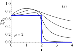
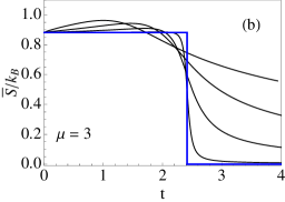
In Figs. 4 and 5 we show the dependence of helicity and entropy on the growth parameter $t$ at fixed nucleation parameter $\tau$ (five curves) and range parameter $\mu$ (two panels).

Figure 4: (Color online) Helicity $\bar{N}_{\mathrm{hl}}$ versus growth parameter $t$ at values $\tau=1,0.25,0.05,0.0025$ (thin lines) and $\tau=0$ (thick line) of the nucleation parameter for (a) $\mu=2$ and (b) $\mu=3$.

Figure 5: (Color online) Entropy $\bar{S}/k_{\mathrm{B}}$ versus $t$ at $\tau=1,0.25,0.05,0.0025$ (thin lines) and $\tau=0$ (thick line) for (a) $\mu=2$ and (b) $\mu=3$.

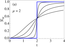
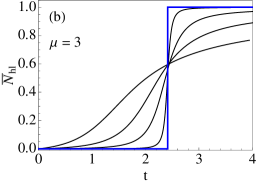
At finite cooperativity $(\tau>0)$ the helicity crosses over from a low to a high value near $t_{0}$. The rise in helicity becomes sharper with increasing cooperativity and turns into a step discontinuity in the limit $\tau\to 0$. Analytically, expression (40) with (36) substituted yields

$$\bar{N}_{\mathrm{hl}}=\theta\!\left(t-t_{0}\right)\qquad(\tau=0).$$ (42)

While order as reflected in the helicity increases monotonically with $t$, the disorder as reflected in the entropy is not monotonically decreasing. It shows a shallow maximum at $t\simeq 1$ separate from the shoulder at $t\simeq t_{0}$. The reason for this difference is that there is only one source of order – helical links – but two sources of disorder: disorder inside coil segments and disorder in the sequence of helical/coil segments of diverse lengths. It is the first source of disorder that produces the shoulder and the second source that produces the shallow maximum. The Zimm-Bragg case $\mu=1$ is pathological in this respect. It produces coil segments without internal entropy as noted and commented on before [28].

As $\tau\to 0$, the segments grow larger in size and become fewer in numbers (see Sec. 4.2 below). This reduces disorder of the second kind. At infinite cooperativity the entropy turns into a step discontinuity of height and location. Expression (41) with (36) substituted becomes

$$\frac{\bar{S}}{k_{B}}=\theta\!\left(t_{0}-t\right)\ln t_{0}\qquad(\tau=0).$$ (43)

This discontinuity signals the presence of a latent heat (see Sec. 4.3 below).

Next we investigate the same measures of order and disorder as functions of $t$ at fixed $\tau=1.0$ (low cooperativity) or $\tau=0.2$ (high cooperativity) for increasing numbers $\mu$ of coil states per residue including the limit $\mu\to\infty$. Our results are shown in Figs. 6 and 7. The crossover behavior for small $\mu$ turns into a continuous order-disorder transition as $\mu\to\infty$.

Figure 6: (Color online) Helicity $\bar{N}_{\mathrm{hl}}$ versus growth parameter $t$ at cooperativity (a) $\tau=1.0$ and (b) $\tau=0.2$ for $\mu=2,3,4,9$ (thin curves from top down) and $\mu=\infty$ (thick curve). The dot-dashed lines marks $t_{\mathrm{c}}$.

Figure 7: (Color online) Entropy $\bar{S}/k_{\mathrm{B}}$ versus $t$ at (a) $\tau=1.0$ and (b) $\tau=0.2$ for $\mu=2,3,4,9$ (thin curves from bottom up) and $\mu=\infty$ (thick curve). The dot-dashed line marks $t_{\mathrm{c}}$.

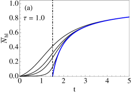
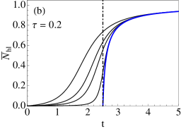
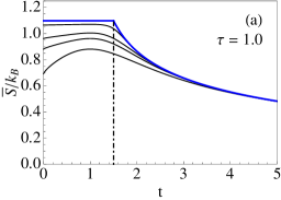
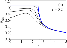
With $\mu$ increasing, the internal source of disorder in coil segments gains dominance over the entropy of mixing between coil and helix segments. The shoulder in $\bar{S}/k_{\mathrm{B}}$ becomes flatter, higher, and sharper. In the limit $\mu\to\infty$ at $t<t_{\mathrm{c}}$, the helicity approaches zero identically and the entropy approaches the value $\bar{S}/k_{\mathrm{B}}=\ln 3$, independent of $\tau$. Disorder defeats order hands down.

The helix phase at $t>t_{\mathrm{c}}$, by contrast, remains a battleground between ordering and disordering tendencies. Both the helicity and the entropy expressions,

$$\bar{N}_{\mathrm{hl}}=1-\frac{t\tau}{\lambda(2\lambda+1-t)},$$ (44)

$$\frac{\bar{S}}{k_{\mathrm{B}}}=\ln\left(1+\frac{\tau}{\lambda}\right) +\frac{t\tau\ln t}{\lambda(2\lambda+1-t)}+\frac{\tau\ln\tau}{\lambda+\tau}\left[\frac{t\tau}{\lambda(2\lambda+1-t)}-1\right],$$ (45)

have linear cusps at $t_{\mathrm{c}}$ with slopes that diverge in the limit $\tau\to 0$. The leading critical singularities at $t_{\mathrm{c}}^{+}$ are

$$\bar{N}_{\mathrm{hl}}=\frac{2t_{0}}{t_{\mathrm{c}}}\frac{t-t_{\mathrm{c}}}{(t_{0}-t_{\mathrm{c}})^{2}}+\mathcal{O}\big{(}(t-t_{\mathrm{c}})^{2}\big{)},$$ (46)

$$\frac{\bar{S}}{k_{\mathrm{B}}} =\ln t_{0}-2\frac{t-t_{\mathrm{c}}}{t_{0}-t_{\mathrm{c}}}\left[\frac{\ln t_{\mathrm{c}}}{t_{0}-t_{\mathrm{c}}}+\frac{\ln(t_{0}-t_{\mathrm{c}})}{t_{\mathrm{c}}}\right]+\mathcal{O}\big{(}(t-t_{\mathrm{c}})^{2}\big{)}.$$ (47)

With the growth parameter increasing from $t_{\mathrm{c}}$ the helicity steeply rises from zero and gradually bends over toward its saturation value whereas the entropy steeply descends from a high value and gradually approaches zero. The plots suggest that cooperativity impedes the onset of ordering, yet assists the quick rise of ordering once it has set in.

4.2 Segments of coil and helix

Further insight into how helical ordering grows during the crossover or near the transition point between conformations can be gained from the two quantities (21) and (22), representing, respectively, the density and average length of segments in one or the other conformation. Coil segments alternate with helix segments. Hence they come in equal numbers. However, their average lengths vary independently with $t$. Parametric representations can be constructed as before. We use (40) and

$$\bar{N}_{\mathrm{seg}}=-\frac{\tau}{w_{1}(1+w_{1})}\frac{\partial w_{1}}{\partial\tau}.$$ (48)

We first examine the $t$-dependence of $\bar{N}_{\mathrm{seg}}$, $L_{\mathrm{cs}}$, and $L_{\mathrm{hs}}$ near the first-order transition that takes place at $t_{0}$ in the limit $\tau\to 0$. Our results for $\mu=2,3$ are shown in Figs. 8 and 9.

Figure 8: Density of segments, $\bar{N}_{\mathrm{seg}}$, versus $t$ at $\tau=1$, $0.25$, $0.05$, $0.0025$ (from top down) for (a) $\mu=2$ and (b) $\mu=3$. The dot-dashed line marks $t_{0}$.

We observe that the density of segments is near zero at small $t$. Here the system is strongly coil-like. The segments grow in numbers with $t$ increasing. They become most numerous at $t_{0}$, where ordering and disordering tendencies compete evenly. The density of segments becomes smaller again as $t$ further increases into the stability regime of the helix conformation. The maximum of $\bar{N}_{\mathrm{seg}}$ at $t_{0}$ strongly depends on $\tau$. In the limit $\tau\to 0$ we have $\bar{N}_{\mathrm{seg}}\equiv 0$, which means that, in a macroscopic system, the number of segments grows more slowly (if at all) than the number of residues.

Figure 9: Average length of coil segments, $L_{\mathrm{cs}}$ (solid lines), and helix segments, $L_{\mathrm{hs}}$ (dashed lines), versus $t$ at $\tau=1$, $0.25$, $0.05,0$ (from bottom up) for (a) $\mu=2$ and (b) $\mu=3$. The dot-dashed line marks $t_{0}$.

Unsurprisingly, $L_{\mathrm{cs}}$ decreases and $L_{\mathrm{hs}}$ increases monotonically with $t$. As expected, both variations are enhanced by cooperativity. Most interesting is the limit $\tau\to 0$. The exact expressions for the average lengths of helix segments at $t<t_{0}$ and coil segments at $t>0$ read

$$L_{\mathrm{hs}} =\frac{t_{0}}{t_{0}-t},$$ (49)

$$L_{\mathrm{cs}} =\frac{t}{(1+t)(3-t)}\Bigg{[}\frac{2(\mu+1)}{r_{\mu}(t-1)}+2\mu r_{\mu}(t-1)-(2\mu+1)(t-1)\Bigg{]},$$ (50)

respectively, with $r_{\mu}(w)$ from (28). Both expressions diverge $\propto|t-t_{0}|^{-1}$ as $t$ approaches $t_{0}$ from opposite sides and then stay infinite.

These results tell us that the macrostate with zero helicity and saturated entropy at $t<t_{0}$ still contains helix segments albeit only in numbers that do not add up to a nonzero density but still produce a well-defined average size. They coexist with an equal number of coil segments of macroscopic lengths. Conversely, the macrostate of zero entropy (per residue) and saturated helicity at $t>t_{0}$ is not a single helical domain. Here helix segments of short average length in numbers that amount to zero density coexist with an equal number of helix segments of macroscopic lengths.

A different picture emerges near the second-order transition at $t=t_{\mathrm{c}}$ in the limit $\mu\to\infty$. Results for the density of segments at high and low cooperativity are shown in Fig. 10 and results for their average lengths in Fig. 11. This includes numerical results for $\mu<\infty$ and analytical results for $\mu=\infty$.

Figure 10: (Color online) Density of segments, $\bar{N}_{\mathrm{seg}}$, versus $t$ at (a) $\tau=1.0$ and (b) $\tau=0.2$ for $\mu=2,3,4,9$ (thin curves lines left to right) and $\mu=\infty$ (thick curve). The dot-dashed line marks $t_{\mathrm{c}}$.

Figure 11: (Color online) Average length of coil segments, $L_{\mathrm{cs}}$ (solid lines), and helix segments, $L_{\mathrm{hs}}$ (dashed lines), for $\mu=2$ (thin lines) and $\mu=\infty$ (thick lines) versus $t$ at (a) $\tau=1.0$ and (b) $\tau=0.2$. The dot-dashed line marks $t_{\mathrm{c}}$.

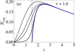
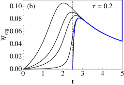
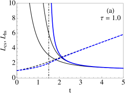
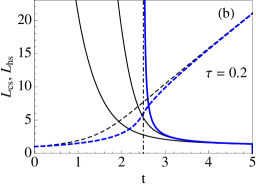
The density of segments vanishes identically in the coil phase $(t<t_{\mathrm{c}})$ and then rises in a linear cusp to a smooth maximum in the helix phase $(t>t_{\mathrm{c}})$ :

$$\bar{N}_{\mathrm{seg}}=\frac{\tau}{\lambda+\tau}\left[1-\frac{t\tau}{\lambda(2\lambda+1-t)}\right]=\frac{2t_{0}}{t_{\mathrm{c}}}\frac{t-t_{\mathrm{c}}}{t_{0}-t_{\mathrm{c}}}+\mathcal{O}\big{(}(t-t_{\mathrm{c}})^{2}\big{)}.$$ (51)

The average length of coil segments in the helix phase,

$$L_{\mathrm{cs}}=\frac{t(\lambda+\tau)}{\lambda(2\lambda+1-t)-t\tau}=\frac{t_{\mathrm{c}}}{2}\frac{t_{0}-t_{\mathrm{c}}}{t-t_{\mathrm{c}}}+\frac{2t_{\mathrm{c}}^{2}-9t_{\mathrm{c}}+15}{4(t_{0}-t_{\mathrm{c}})}+\mathcal{O}(t-t_{\mathrm{c}}),$$ (52)

diverges at $t_{\mathrm{c}}^{+}$ and remains infinite in the coil phase. The average length of helix segments, by contrast, remains finite in both phases,

$$L_{\mathrm{hs}}=\left\{\begin{array}[]{ll}{\displaystyle\frac{t_{0}}{t_{0}-t}}&:t\leq t_{\mathrm{c}},\\ \rule[-5.69054pt]{0.0pt}{22.76219pt}{\displaystyle 1+\frac{\lambda}{\tau}}&:t\geq t_{\mathrm{c}},\end{array}\right.$$ (53)

where again, $t_{0}=3$ for $\mu=\infty$ in (51)-(53). The graph of $L_{\mathrm{hs}}$ is continuous and smooth at $t_{\mathrm{c}}$. The singularity is of higher order. Only in the helix phase does the shape of the curve depend on $\tau$.

The most striking feature in the data shown concerns the helix segments. Unlike in the case of the first-order transition, the ordered phase near $t_{\mathrm{c}}$ supports a significant density of coil and helix segments of comparable finite size. The average length of helix segments depends only weakly on $\mu$ and only moderately on $\tau$, in strong contrast to the average length of coil segments, which exhibits strong dependences on both parameters.

4.3 Heat capacity and latent heat

The heat capacity, $\bar{C}\doteq T(\partial\bar{S}/\partial T)_{\epsilon_{\mathrm{n}},\epsilon_{\mathrm{g}}}$, illuminates the competition between order and disorder from yet a different angle. From (41) we derive

$$\frac{\bar{C}}{k_{B}}=\frac{2w_{1}+1}{w_{1}^{2}(1+w_{1})^{2}}\left[t\ln t\frac{\partial w_{1}}{\partial t}+\tau\ln\tau\frac{\partial w_{1}}{\partial\tau}\right]^{2}-\frac{1}{w_{1}(1+w_{1})}\left[t(\ln t)^{2}\frac{\partial w_{1}}{\partial t}\right.$$

$$\hskip 28.45274pt\left.+\tau(\ln\tau)^{2}\frac{\partial w_{1}}{\partial\tau}+(t\ln t)^{2}\frac{\partial^{2}w_{1}}{\partial t^{2}}+(\tau\ln\tau)^{2}\frac{\partial^{2}w_{1}}{\partial\tau^{2}}+2(t\ln t)(\tau\ln\tau)\frac{\partial^{2}w_{1}}{\partial t\partial\tau}\right].$$ (54)

Figure 12 shows the dependence of the heat capacity on the growth parameter for the case $\mu=2$ at moderate to high cooperativity and for the case $\mu=\infty$ over a wider range of cooperativity.

Figure 12: Heat capacity $\bar{C}/k_{\mathrm{B}}$ versus $t$ for (a) $\mu=2$ at $\tau=0.05$, $0.025$, $0.01$, $0.005$ (from top down on the right in the main plot and from bottom up in the inset) and (b) $\mu=\infty$ at $\tau=1.0$, $0.5$, $0.25$, $0.2$ (from bottom up in main plot) and $\tau=0.2$, $0.1$, $0.05$, $0.01$ (from top down in the inset). The dot-dashed lines mark $t_{c}$ for given $\tau$.

At $t<t_{0}=2$ in panel (a) we observe a weak signal that is associated with the entropy caused by alternating coil and helix segments as discussed previously. This contribution fades away at high cooperativity (best seen in the inset) as the density of segments diminishes. The peak at $t\gtrsim t_{0}$, on the other hand, is associated with the entropy inside coil segments. With increasing cooperativity, this contribution grows in a more and more narrow range at $t_{0}$. Similar structures have been obtained in recent Monte Carlos simulations, albeit upon variation of temperature and in a somewhat different scenario [29].

In the limit $\tau\to 0$ for $\mu<\infty$, where the coil-helix crossover sharpens into a first-order transition at $t_{0}$, the heat capacity approaches zero everywhere except at the transition point, where it diverges and produces, via (43), a latent heat of magnitude $\epsilon_{\mathrm{g}}$. Conversely, in the limit $\mu\to\infty$ at $\tau>0$, where the coil-helix crossover turns into a second-order transition at $t_{\mathrm{c}}$, the heat capacity approaches zero in the coil conformation and remains nonzero in the helix conformation as shown in panel (b). When the transition changes from second to first order when $\tau\to 0$ for $\mu=\infty$, implying $t_{\mathrm{c}}\to t_{0}=3$, the heat capacity throughout the helix conformation approaches zero as illustrated in the inset.

5 Conclusion and outlook

We have launched this project mainly for the purpose of interpreting (ongoing and projected) experiments on pHLIP. In this first of three stages of analysis we have constructed a microscopic model for the pH-driven coil-helix conformational change of a long polypeptide adsorbed to a water-lipid interface. We have employed a methodology that facilitates the exact statistical mechanical analysis of our model. The three model parameters $t,\tau,\mu$ have settings for which the conformation changes either in a crossover, a first-order transition, or a second-order transition.

We have carried out the analysis to the extent needed for a discussion of the sources and agents of order and disorder. Our results include the $t$-dependence of the helicity (order parameter), the average numbers and the average lengths of helix and coil segments, the entropy, and the heat capacity. The behavior of these quantities near the continuous or the discontinuous transition has been given special attention. We have plotted all quantities versus $t$ at constant $\tau$ and $\mu$ for a reason. The experimentally relevant processes for which we use our model will primarily involve variations of the growth parameter $t$. These variations are caused by changes in pH. The targeted peptides, adsorbed to the water-lipid interface, include side chains that are strongly hydrophobic (e.g. Leu) and side chains that are negatively charged (e.g. Asp, Glu).

A drop in pH leads to the protonation of the negatively charged side chains and, therefore, enhances the overall hydrophobicity. The backbone of a coil segment thus pushed past the lipid headgroups is now more likely to satisfy an H-bond internally than externally. The enthalpic cost for broken internal H-bonds increases. This cost is encoded in $t$. Any increase in $t$ favors a growth of helix segments at the expense of coil segments. A rise in pH has the opposite effect. The value of $t$ decreases. Coil segments grow at the expense of helix segments.

The cooperativity parameter $\tau$, by contrast, is much less sensitive to a change in pH. In the nucleation process of coil segments from the helix conformation, for example, the internal H-bonds are much more isolated from environmental influences than are those at the border between coil segments and helix segments.

At this point, our project has reached a fork, where natural continuations point in two different directions and address the interests of somewhat different audiences. These continuations, already in the works, are outlined as follows.

5.1 Heterogeneous environment and short peptides

In one continuation we begin by considering long polypeptides that are no longer confined to a plane parallel to a flat water-lipid interface. The growth parameter $t$, which drives the conformational change, then becomes a field $t(x)$ and acquires a profile that depends on the local medium. Here $x$ is a position coordinate in the direction perpendicular to the plane of the membrane. Such circumstances pose a serious challenge to any existing model and its method of analysis. However, the methodology used here is well positioned in that respect. It has already been proven (in different applications [25, 27, 30]) to be adaptable to heterogeneous environments.

The shape of the parameter field $t(x)$ will be determined by the availability of polar molecules to satisfy external H-bonds along the backbone of the peptide. The dominant factor that shapes the field $t(x)$ will be the density profile $\rho_{\mathrm{w}}(x)$ across the membrane, for which data from experiments [31] and simulations [32] are available. Subdominant factors include electrostatic interactions and fluid-mechanical properties of lipids.

From the analysis of our extended model emerge profiles for the densities of free energy, enthalpy, entropy, and helicity of long polypeptides that traverse the heterogeneous environment (ranging from polar to non-polar) along some path that is subject to conformational constraints [33]. These profiles, in turn, will be interpreted as propensities for the statistical mechanical behavior of short peptides in the same environment.

At this stage of the analysis, additional enthalpic and entropic effects involving the side chains, the semi-fluid bilayer of lipid amphiphiles, and the hydrogen-bonded network of $\mathrm{H_{2}O}$ molecules can be built into the model. The outcome are landscapes of free energy, enthalpy, entropy, and helicity for short peptides of specific composition. The free-energy landscapes in particular then set the stage for (i) a theoretical study of the kinetics of trans-membrane insertion and exit of pHLIP and other membrane peptides and (ii) a direct comparison with experiments currently in progress that investigate the insertion/exit processes of pHLIP via tryptophan fluorescence and the accompanying conformational changes via circular dichroism spectroscopy.

This first continuation can also benefit from recent studies in the same area of research. Not yest included in our modeling are effects related to torsion and tension, which are bound to be present in the heterogeneous membrane environment. Experimental, computational, and analytic studies of force-extension and torque-twist characteristics and the associated steric constraints [34, 35, 36, 37] will be of great value for that purpose. The kinetic modeling of pHLIP insertion while undergoing a conformational change will find valuable guidance from recent studies that have investigated the fluctuation properties of helical polymers in confined environments including narrow channels [38, 39, 40] and studies that have investigated the Brownian dynamics of polymers in the membrane environment [41].

5.2 Extensions of analysis, model, and scope

A second continuation focuses on the statistical mechanics of phase transitions and critical singularities in the context of the microscopic model presented in this work and extensions thereof. It is well known that the presence of a phase transition at nonzero temperature in a system that is, in some sense, one-dimensional requires interactions of long-range to stabilize an ordered phase in the face of strong thermal fluctuations. In our model, which is truly microscopic and analyzed exactly, this stabilizing agent comes in the form of quasiparticles that extend over entire coil segments (hosts) or over parts thereof (hybrids).

In the context of the experiments that motivated this work we have examined conformational changes driven by the control parameter $t$ at fixed $\tau,\mu$ as reflected in just a few relevant quantities. The phase transitions that occur in the limits $\tau\to 0$ (first-order) or $\mu\to\infty$ (second order) produce different singularities in other quantities of no less interest for the statistical mechanical analysis. Such quantities of general interest include a mechanical response function, a correlation length, and a correlation function. The further analysis of critical exponents and scaling laws is best presented in a more general framework and along with model extensions that remain inside the reach of our method of exact analysis.

In a final note, we should like to draw the reader’s attention to a different set of applications, for which our statistical mechanical model and its extensions are likely to produce significant new insights. These applications investigate the statistical mechanics and the dynamics of DNA melting (thermal denaturation) [13, 14, 42, 43, 44, 45, 46, 47, 48] or the loop formation in RNA [49]. Of particular interest is the loop exponent in the configurational entropy of loop formation [14, 49], which is frequently used as an adjustable parameter. The further development of our project aims for the analytic calculation of loop exponents pertaining to realistic scenarios. Discussions of and debates about crossovers, first-order transitions, and second-order transitions are at the center of most of these studies. The transcription and adaptation of our methodology to this particular physics context is already in progress. The main challenge in the endeavor is the extension of the self-avoiding random walk to three dimensions.

Appendix A Polynomial equations

The $2\mu$ Eqs. (8) with the $\beta\epsilon_{m}$ expressed via parameters (10) and (11) and the $g_{mm^{\prime}}$ as stated in Sec. 2.2 acquire the following form (for $\mu\geq 2$):

$$\frac{t}{\tau} =\frac{w_{1}^{2}}{1+w_{1}}\frac{1+w_{2}}{w_{2}}\frac{1+w_{\mu+1}}{w_{\mu+1}},$$ (55)

$$t^{2} =(1+w_{m})\frac{w_{1}^{2}}{(1+w_{1})^{2}}\frac{1+w_{m+1}}{w_{m+1}}\frac{1+w_{\mu+m-1}}{w_{\mu+m-1}}\frac{1+w_{\mu+m}}{w_{\mu+m}},\quad m=2,...,\mu-1$$ (56)

$$t^{2} =(1+w_{\mu})\frac{w_{1}^{2}}{(1+w_{1})^{2}}\frac{1+w_{2\mu-1}}{w_{2\mu-1}}\frac{1+w_{2\mu}}{w_{2\mu}},$$ (57)

$$t =(1+w_{m})\frac{w_{1}}{1+w_{1}},\qquad m=\mu+1,...,2\mu.$$ (58)

From (58) we infer

$$w_{\mu+1}=...=w_{2\mu}\doteq w,$$ (59)

which, upon substitution, simplifies (55)-(58) into

$$\frac{t}{\tau} =\frac{w_{1}^{2}}{1+w_{1}}\frac{1+w_{2}}{w_{2}}\frac{1+w}{w},$$ (60)

$$t^{2} =(1+w_{m})\frac{w_{1}^{2}}{(1+w_{1})^{2}}\frac{1+w_{m+1}}{w_{m+1}}\frac{(1+w)^{2}}{w^{2}},\quad m=2,...,\mu-1,$$ (61)

$$t^{2} =(1+w_{\mu})\frac{w_{1}^{2}}{(1+w_{1})^{2}}\frac{(1+w)^{2}}{w^{2}},$$ (62)

$$t =(1+w)\frac{w_{1}}{1+w_{1}}.$$ (63)

Substitution of (63) into (60)-(62) yields

$$w_{1} =\frac{w}{\tau}\frac{w_{2}}{1+w_{2}},\quad\tau\neq 0,$$ (64)

$$w_{m} =w^{2}\frac{w_{m+1}}{1+w_{m+1}}-1,\quad m=2,...,\mu-1,$$ (65)

$$w_{\mu} =w^{2}-1,$$ (66)

which express all $w_{m}$ for $m\leq\mu$ from $w$ recursively.

Next we show that these recursive relations can be satisfied by Chebyshev polynomials of the second kind, which themselves are generated recursively from $S_{0}(w)=1$ and $S_{1}(w)=w$ via

$$S_{m+2}(w)=wS_{m+1}(w)-S_{m}(w),\quad m=0,1,2,\ldots$$ (67)

We reason inductively by writing (66) in the form

$$w_{m}=\frac{S_{\mu-m+2}(w)}{S_{\mu-m}(w)},\quad m=\mu.$$ (68)

If (68) holds for some $m$ then we infer from (65) that it also holds for $m-1$:

$$w_{m-1} =w^{2}\frac{w_{m}}{1+w_{m}}-1=\frac{w^{2}S_{\mu-m+2}(w)}{S_{\mu-m+2}(w)+S_{\mu-m}(w)}-1$$ (69)

$$=\frac{wS_{\mu-m+2}(w)-S_{\mu-m+1}(w)}{S_{\mu-m+1}(w)}=\frac{S_{\mu-m+3}(w)}{S_{\mu-m+1}(w)}.$$

This validates (68) for $m=2,\ldots,\mu$. We use (64) to obtain

$$w_{1}=\frac{S_{\mu}(w)}{\tau S_{\mu-1}(w)}.$$ (70)

The polynomial equation that determines $w$,

$$(1+w-t)S_{\mu}(w)=t\tau S_{\mu-1}(w),$$ (71)

follows from (63) substituted in (70). This completes the derivation of (12) and (2.3). All $w_{m}$ must be non-negative to be physically meaningful. Only one root of (71) satisfies this criterion.

Appendix B Particle population densities

The solution of the linear Eqs. (9) yields the following explicit expressions for the population densities of statistically interacting particles:

$$\bar{N}_{m} =\frac{S_{\mu-m}(w)S_{\mu-m+1}(w)}{\gamma_{\mu}},$$

$$\bar{N}_{\mu+m} =\frac{[S_{\mu-m}(w)]^{2}}{\gamma_{\mu}},\quad m=1,\ldots,\mu,$$ (72)

$$\gamma_{\mu} \doteq(1+w)\!\left[\,\sum_{m=0}^{\mu-1}\big{[}S_{m}(w)\big{]}^{2}+\frac{\big{[}S_{\mu}(w)\big{]}^{2}}{t\tau}\,\right],$$ (73)

$$=(1+w)\left[\frac{2\mu+1-S_{2\mu}(w)}{4-w^{2}}+\frac{\big{[}S_{\mu}(w)\big{]}^{2}}{t\tau}\right].$$

Entropy (18), enthalpy (19), helicity (20), and density of segments (21) can all be expressed in terms of the $\bar{N}_{m}$:

$$\frac{\bar{S}}{k_{\mathrm{B}}}=\sum_{m=1}^{2\mu}\bar{N}_{m}\Big{[}(1+w_{m})\ln(1+w_{m})-w_{m}\ln w_{m}\Big{]},$$ (74)

$$\bar{H}=\sum_{m=1}^{2\mu}\bar{N}_{m}\epsilon_{m},$$ (75)

$$\bar{N}_{\mathrm{seg}}=\bar{N}_{1}=\frac{\big{[}S_{\mu}(w)\big{]}^{2}}{\gamma_{\mu}}\frac{w+1-t}{t\tau},$$ (76)

$$\bar{N}_{\mathrm{hl}}=1-\bar{N}_{1}-2\sum_{m=2}^{\mu}\bar{N}_{m}-\sum_{m=\mu+1}^{2\mu}\bar{N}_{m}=\frac{\big{[}S_{\mu}(w)\big{]}^{2}}{\gamma_{\mu}}\frac{w+1}{t\tau},$$ (77)

The shortest proof of (B) uses its substitution into a scaled version of (9),

$$w_{m^{\prime}}\bar{N}_{m^{\prime}}=\sum_{m=1}^{\mu}\big{(}g_{m^{\prime}m}\bar{N}_{m}+g_{m^{\prime},m+\mu}\bar{N}_{m+\mu}\big{)}=\delta_{1m^{\prime}}.$$ (78)

We perform this substitution in four batches: (i) for $m^{\prime}=2\mu$ we use $g_{2\mu,m}=-\delta_{\mu m}$; (ii) for $m^{\prime}=\mu+m^{\prime\prime}$, $m^{\prime\prime}=1,\ldots,\mu-1$ we use $g_{\mu+m^{\prime\prime},m}=-\delta_{m^{\prime\prime}m}-\delta_{m^{\prime\prime},m-1}$; (iii) for $m^{\prime}=2,\ldots,\mu$ we use $g_{m^{\prime}m}=-\delta_{m^{\prime},m+1}$; and (iv) for $m^{\prime}=1$ we use $g_{1m}=2$, $g_{1,\mu+m}=1$, $m=1,\ldots,\mu$.

In the first three batches (78) is shown to be satisfied by merely using (2.3) and (67):

$$\mathrm{(i)}:~{}w[S_{0}(w)]^{2}-S_{0}(w)S_{1}(w)=0,$$ (79)

$$\mathrm{(ii)}:~{} w[S_{\mu-m^{\prime\prime}}(w)]^{2}-S_{\mu-m^{\prime\prime}}(w)S_{\mu-m^{\prime\prime}+1}(w)-S_{\mu-m^{\prime\prime}-1}(w)S_{\mu-m^{\prime\prime}}(w)=0,$$ (80)

$$\mathrm{(iii)}:~{} \frac{S_{\mu-m^{\prime}+2}(w)}{S_{\mu-m^{\prime}}(w)}S_{\mu-m^{\prime}}(w)S_{\mu-m+1}(w)-S_{\mu-m^{\prime}+1}(w)S_{\mu-m+2}(w)=0.$$ (81)

In the fourth batch, (78) reduces to the identity,

$$\mathrm{(iv)}:~{} \frac{[S_{\mu}(w)]^{2}}{\tau}+2\sum_{m=1}^{\mu}S_{m-1}(w)S_{m}(w)+\sum_{m=1}^{\mu}[S_{m-1}(w)]^{2}=\gamma_{\mu},$$ (82)

which is proven by also using (12).

The two sources of disorder identified in Sec. 4.1, namely the disorder in the sequence of coil/helix segments of diverse lengths and disorder within individual coil segments, are related to the population densities $\bar{N}_{m}$ of $2\mu$ species of particles from three catgories (hosts, hybrids, and tags).

Hosts $(m=1)$ generate coil segments out of the helix pseudo-vacuum whereas hybrids $(m=2,\ldots,\mu)$ and tags $(m=\mu+1,\ldots,2\mu)$ extend coil segments at the expense of helix segments. Thermally excited hosts at random locations along the polypeptide helix thus produce one source of disorder and germinate the other source of disorder via the thermal excitation of hybrids and tags nested inside.

Each coil segment, nucleated by exactly one host particle, forms a self-avoiding random walk assembled from hybrids and tags. The distribution of hybrids and tags inside a large coil segment as realized in the limit $\tau\to 0$ at $t<t_{0}$ and inferred from (B), reads

$$\bar{N}_{m} =\frac{2\sin\big{(}(m-1)\phi_{0}\big{)}\sin\big{(}m\phi_{0})}{(\mu+1\big{)}t_{0}},$$

$$\bar{N}_{\mu+m} =\frac{2\sin^{2}\!\big{(}m\phi_{0})}{(\mu+1\big{)}t_{0}},\quad m=1,\ldots,\mu,$$ (83)

where $\phi_{0}=\pi/(\mu+1)$. In the limit $\mu\to\infty$, the distributions of both hybrids and tags acquire identical $\sin^{2}x$ density profiles if we set $x=m/\mu$ for hybrids and $x=(\mu+m)/\mu$ for tags.

References

- [1] J. L. Popot and D. M. Engelman, Biochemistry 29, 4031 (2001).
- [2] S. H. White and W. C. Wimley, Annu. Rev. Biophys. Biomol. Struct. 28, 319 (1999).
- [3] D. M. Engelman, Y. Chen, C. N. Chin, A. R. Curran, A. M. Dixon, A. D. Dupuy, A. S. Lee, U. Lehnert, E. E. Matthews, Y. K. Reshetnyak, A. Senes, and J. L. Popot, FEBS Lett. 555, 122 (2003).
- [4] A. S. Ladokhin and S. H. White, Biochemistry 43, 5782 (2004).
- [5] Y. K. Reshetnyak, M. Segala, O. A. Andreev, and D. M. Engelman, Biophys. J. 93, 2363 (2007).
- [6] D. Weerakkody, A. Moshnikova, M. S. Thakur, O. A. Andreev, and Y. K. Reshetnyak, Proc. Natl. Acad. Sci. USA 110, 5834 (2013).
- [7] Y. K. Reshetnyak, O. A. Andreev, M. Segala, V. S. Markin, and D. M. Engelman, Proc. Natl. Acad. Sci. USA 105, 15340 (2008).
- [8] O. A. Andreev, A. G. Karabazhak, D. Weerakkody, G. O. Andreev, D. M. Engelman, and Y. R. Reshetnyak, Proc. Natl. Acad. Sci. USA 107, 4081 (2010).
- [9] A. G. Karabadzhak, D. Weerakkody, D. Wijwsinghe, M. S. Thakur, D. M. Engelman, O. A. Andreev, V. S. Markin, and Y. R. Reshetnyak, Biophys. J. 102, 1846 (2012).
- [10] D. Poland and H. A. Scheraga, Theory of Helix-Coil Transitions in Biopolymers (Academic Press, New York, 1970).
- [11] B. H. Zimm and J. K. Bragg, J. Chem Phys. 31, 526 (1959).
- [12] S. Lifson, J. Chem. Phys. 40, 3705 (1964).
- [13] D. Poland and H. A. Scheraga J. Chem Phys. 45, 1436, 1464 (1966).
- [14] M. E. Fisher, J. Chem. Phys. 45, 1469 (1966).
- [15] F. D. M. Haldane, Phys. Rev. Lett. 67, 937 (1991).
- [16] Y.-S. Wu, Phys. Rev. Lett. 73, 922 (1994).
- [17] S. B. Isakov, Phys. Rev. Lett. 73, 2150 (1994); Mod. Phys. Lett. B 8, 319 (1994).
- [18] D.-V. Anghel, J. Phys. A 40, F1013 (2007); Europhys. Lett. 87, 60009 (2009).
- [19] G. G. Potter, G. Müller, and M. Karbach, Phys. Rev. E 75, 061120 (2007); 76, 061112 (2007).
- [20] P. Lu, J. Vanasse, C. Piecuch, M. Karbach, and G. Müller, J. Phys. A 41, 265003 (2008).
- [21] D. Liu, P. Lu, G. Müller, and M. Karbach, Phys. Rev. E 84, 021136 (2011).
- [22] P. Lu, D. Liu, G. Müller, and M. Karbach Condens. Matter Phys. 15, 13001 (2012).
- [23] D. Liu, J. Vanasse, G. Müller, and M. Karbach, Phys. Rev. E 85, 011144 (2012).
- [24] N. Gundlach, M. Karbach, D. Liu, and G. Müller, J. Stat. Mech. P04018 (2013).
- [25] C. Moore, D. Liu, B. Ballnus, M. Karbach, and G. Müller J. Stat. Mech. P04008 (2014).
- [26] B. Bakhti, M. Karbach, P. Maass, M. Mokim, and G. Müller, Phys. Rev. E 89, 012137 (2014).
- [27] Y. Öz, N. Gundlach, M. Karbach, P. Lu, and G. Müller Molecular Chains under Tension and Torque: Force-Extension and Torque-Twist Characteristics (unpublished).
- [28] C. Nowak, V. G. Rostiashvili, and T. A. Vilgis, J. Chem. Phys. 126, 034902 (2007).
- [29] Y. Chen, Q. Zhang, and J. Ding, J. Chem. Phys. 120, 3467 (2004).
- [30] B. Bakhti, P. Maass, and G. Müller, Interacting hard rods in heterogeneous environment (unpublished).
- [31] K. Åman, E. Lindahl, O. Edholm, P. Håkansson, and P.-O. Westlund, Biophys. J. 84, 102 (2003).
- [32] J. L. MacCallum, W. F. D. Bennett, and D. P. Tieleman, Biophys. J. 98, 3393 (2008).
- [33] Y. K. Reshetnyak, Oleg. A. Andreev, M. Karbach, and G. Müller, Landscapes of Free Energy, Enthalpy, and Entropy for Peptides in Membrane Environment (unpublished).
- [34] M. N. Tamashiro and P. Pincus, Phys. Rev. E 63, 021909 (2001).
- [35] F. Hanke , A. Serr , H. J. Kreuzer and R. R. Netz, Eur. Phys. Lett. 92, 53001 (2010).
- [36] B. Chakrabarti and A. J. Levine, Phys. Rev. E 71, 031905 (2005).
- [37] B. Chakrabarti and A. J. Levine, Phys. Rev. E 74, 031903 (2006).
- [38] A. Lamura, T. W. Burkhardt, and G. Gompper, Phys. Rev. E 70, 051804 (2004).
- [39] Y. Yang, T. W. Burkhardt, and G. Gompper, Phys. Rev. E 76, 011804 (2007).
- [40] T. W. Burkhardt, Y. Yang, and G. Gompper, Phys. Rev. E 82, 041801 (2010).
- [41] S. Ramachandran, S. Komura, K. Seki, and G. Gompper, Eur. Phys. J. E 34: 46 (2011).
- [42] M. Peyrard, and A. R. Bishop, Phys. Rev. Lett. 62, 2755 (1989).
- [43] T. Dauxois, M. Peyrard, and A. R. Bishop, Phys. Rev. E 47, R44, 684 (1993).
- [44] N. Theodorakopoulos, T. Dauxois, and M. Peyrard, Phys. Rev. Lett. 85, 6 (2000).
- [45] Y. Kafri, D. Mukamel, and L. Peliti, Phys. Rev. Lett. 85, 4988 (2000).
- [46] M. S. Causo, B. Coluzzi, and P. Grassberger, Phys. Rev. E 62, 3958 (2000).
- [47] D. Cule and T. Hwa, Phys. Rev. Lett. 79, 2375 (1997).
- [48] E. Carlon, E. Orlandini, and L. Stella, Phys. Rev. Lett. 88, 198101 (2002).
- [49] T. R. Einert and R. R. Netz, Biophys. J. 100, 2745 (2011).