Associative Networks with Diluted Patterns: Dynamical Analysis at Low and Medium Load

S Bartolucci1, A Annibale 1,2 1 Department of Mathematics, King’s College London, The Strand, London WC2R 2LS, UK 2 Institute for Mathematical and Molecular Biomedicine, King’s College London, Hodgkin Building, London SE1 1UL, UK
(March 13, 2024)
Abstract

In this work we solve the dynamics of pattern diluted associative networks, evolving via sequential Glauber update. We derive dynamical equations for the order parameters, that quantify the simultaneous pattern recall of the system, and analyse the nature and stability of the stationary solutions by means of linear stability analysis as well as Monte Carlo simulations. We investigate the parallel retrieval capabilities of the system in different regions of the phase space, in particular in the low and medium storage regimes and for finite and extreme pattern dilution. Results show that in the absence of patterns cross-talk, all patterns are recalled symmetrically for any temperature below criticality, while in the presence of pattern cross-talk, symmetric retrieval becomes unstable as temperature is lowered and a hierarchical retrieval takes over. The shape of the hierarchical retrieval occurring at zero temperature is provided. The parallel retrieval capabilities of the network are seen to degrade gracefully in the regime of strong interference, but they are not destroyed.

1 Introduction

Associative networks with diluted patterns have been recently introduced [1] as a generalisation of the standard Hopfield model [2, 3, 4]. Interestingly, the introduction of dilution in the stored patterns of information, drastically changes the collective behaviour of the system, switching its operational behaviour from sequential to parallel processing. In fact, pattern diluted associative networks are able to orchestrate a parallel retrieval of multiple patterns of information at the same time. Despite their wide range of possible applications, from artificial intelligence [5] to theoretical immunology [6], these types of memories have been studied analytically only in statics so far, where several dilution and storage regimes were investigated [7, 8, 9]. Dynamical studies are limited to numerical simulations and are restricted to the low storage regime, where the number of stored patterns is finite [10]. While lacking so far, the dynamical approach is generally expected to provide richer information than static analysis, which can only describe the behaviour of the system at the steady state, and it does not require that the system is in equilibrium. In this work we carry out a dynamical analysis of associative memories with diluted patterns, evolving via Glauber sequential update. We solve the dynamics in different storage regimes, via non-equilibrium statistical mechanical techniques, first developed in [11, 12] for standard Hopfield networks and spin glasses. We derive equations for the time evolution of a set of macroscopic order parameters, quantifying the simultaneous patterns retrieval, from the dynamical laws of the microscopic neuronal system. We analyse the structure of the stationary solutions of the dynamics in different regimes of dilution (from finite to extreme), in the low and in the medium storage regimes, and we inspect their stability, in different regions of the phase diagram, through linear stability analysis as well as Monte Carlo simulations. Our analysis clarifies several results from previous equilibrium analysis, establishing the limit of their validity in different regions of the tunable parameters space (noise, dilution and storage load). Moreover, it provides new information in those regions of the phase space where previous results from equilibrium analysis correspond to unstable steady states of the dynamical equations. As a result, this work draws a complete picture of the rich dynamical behaviour of pattern diluted associative networks away from saturation.

The paper is organised as follows. In Sec. 2 we define the model and its microscopic dynamics. In Sec. 3 we derive dynamical equations for a suitable set of macroscopic parameters, which quantify the (parallel) retrieval of the system, and we lay the basis for the analysis of the nature and stability of stationary solutions in different regimes of dilution and storage load. Sec. 4 is devoted to low storage and finite dilution, while Sec. 5 deals with the analysis at medium load and extreme dilution. Finally, in Sec. 6 we summarise and discuss our results.

2 The model

We consider a system of N𝑁N Ising spins σi=±1subscript𝜎𝑖plus-or-minus1\sigma_{i}=\pm 1, for i=1,,N𝑖1𝑁i=1,\dots,N, interacting through pairwise couplings

Jij=μ=1Pξiμξjμ,subscript𝐽𝑖𝑗superscriptsubscript𝜇1𝑃superscriptsubscript𝜉𝑖𝜇superscriptsubscript𝜉𝑗𝜇\displaystyle J_{ij}=\sum_{\mu=1}^{P}\xi_{i}^{\mu}\xi_{j}^{\mu}, (1)

where 𝝃μ=(ξ1μ,,ξNμ)superscript𝝃𝜇superscriptsubscript𝜉1𝜇superscriptsubscript𝜉𝑁𝜇{\mbox{\boldmath$\xi$}}^{\mu}=(\xi_{1}^{\mu},\dots,\xi_{N}^{\mu}), with μ=1,,P𝜇1𝑃\mu=1,...,P, represent stored patterns of information. We assume that pattern entries are quenched random variables, identically and independently distributed with probability distribution

P(𝝃)=iμ[c2Nγ(δξiμ,1+δξiμ,1)+(1cNγ)δξiμ,0]𝑃𝝃subscriptproduct𝑖𝜇delimited-[]𝑐2superscript𝑁𝛾subscript𝛿superscriptsubscript𝜉𝑖𝜇1subscript𝛿superscriptsubscript𝜉𝑖𝜇11𝑐superscript𝑁𝛾subscript𝛿superscriptsubscript𝜉𝑖𝜇0\displaystyle P({\mbox{\boldmath$\xi$}})=\prod_{i\mu}\left[\frac{c}{2N^{\gamma}}\big{(}\delta_{\xi_{i}^{\mu},1}+\delta_{\xi_{i}^{\mu},-1}\big{)}+\bigg{(}1-\frac{c}{N^{\gamma}}\bigg{)}\delta_{\xi_{i}^{\mu},0}\right] (2)

where γ[0,1)𝛾01\gamma\in[0,1) and c=𝒪(N0)𝑐𝒪superscript𝑁0c={\mathcal{O}}{(N^{0})}. The number of stored patterns is P=αNδ𝑃𝛼superscript𝑁𝛿P=\alpha N^{\delta}, with δ[0,1)𝛿01\delta\in[0,1), α+𝛼superscript\alpha\in\mathbb{R}^{+}. The fraction of non-zero entries in the stored patterns determines the degree of dilution of the system: for γ=0𝛾0\gamma=0 the system is finitely diluted, whereas for γ>0𝛾0\gamma>0 the system is extremely diluted. For δ>0𝛿0\delta>0 the number of patterns stored in the system diverges in the thermodynamic limit, however as long as δ<1𝛿1\delta<1, the number of patterns grows sub-linearly in the system size, and the system is away from saturation. Spins obey random sequential Glauber dynamics via an effective local field

hi(𝝈)=1N1γjiNJijσjsubscript𝑖𝝈1superscript𝑁1𝛾superscriptsubscript𝑗𝑖𝑁subscript𝐽𝑖𝑗subscript𝜎𝑗\displaystyle h_{i}({{\mbox{\boldmath$\sigma$}}})=\frac{1}{N^{1-\gamma}}\sum_{j\neq i}^{N}J_{ij}\sigma_{j} (3)

so that the probability pt(𝝈)subscript𝑝𝑡𝝈p_{t}({\mbox{\boldmath$\sigma$}}) of finding the system in a state 𝝈=(σ1,,σN)𝝈subscript𝜎1subscript𝜎𝑁{\mbox{\boldmath$\sigma$}}=(\sigma_{1},\dots,\sigma_{N}) at time t𝑡t, evolves according to the master equation

pt(𝝈)t=i=1N[pt(Fi𝝈)wi(Fi𝝈)pt(𝝈)wi(𝝈)]subscript𝑝𝑡𝝈𝑡superscriptsubscript𝑖1𝑁delimited-[]subscript𝑝𝑡subscript𝐹𝑖𝝈subscript𝑤𝑖subscript𝐹𝑖𝝈subscript𝑝𝑡𝝈subscript𝑤𝑖𝝈\displaystyle\frac{\partial{p_{t}(\mbox{\boldmath$\sigma$}})}{\partial{t}}=\sum_{i=1}^{N}\big{[}p_{t}(F_{i}{{\mbox{\boldmath$\sigma$}}})w_{i}(F_{i}{{\mbox{\boldmath$\sigma$}}})-p_{t}(\mbox{\boldmath$\sigma$})w_{i}(\mbox{\boldmath$\sigma$})\big{]} (4)

where Fisubscript𝐹𝑖F_{i} is the i𝑖i-th spin-flip operator Fi(σ1,..,σi,,σN)=(σ1,,σi,σN)F_{i}(\sigma_{1},..,\sigma_{i},...,\sigma_{N})=(\sigma_{1},...,-\sigma_{i},...\sigma_{N}) and transition rates between 𝝈𝝈\sigma and Fi𝝈subscript𝐹𝑖𝝈F_{i}{\mbox{\boldmath$\sigma$}} have the Glauber form

wi(𝝈)=12[1σitanh(βhi(𝝈))]subscript𝑤𝑖𝝈12delimited-[]1subscript𝜎𝑖𝛽subscript𝑖𝝈\displaystyle w_{i}({\mbox{\boldmath$\sigma$}})=\frac{1}{2}[1-\sigma_{i}\tanh{(\beta h_{i}({\mbox{\boldmath$\sigma$}}))}] (5)

where β=1/T𝛽1𝑇\beta=1/T is the inverse temperature of the system, giving the rate of spontaneous spin flips.
For symmetric couplings, as those given in (1), the dynamics obeys detailed balance and the process evolves towards equilibrium, described by the Boltzmann distribution, with Hamiltonian:

H=12N1γi,j=1Nμ=1Pξiμξjμσiσj.𝐻12superscript𝑁1𝛾superscriptsubscript𝑖𝑗1𝑁superscriptsubscript𝜇1𝑃superscriptsubscript𝜉𝑖𝜇superscriptsubscript𝜉𝑗𝜇subscript𝜎𝑖subscript𝜎𝑗\displaystyle H=-\frac{1}{2N^{1-\gamma}}\sum_{i,j=1}^{N}\sum_{\mu=1}^{P}\xi_{i}^{\mu}\xi_{j}^{\mu}\sigma_{i}\sigma_{j}. (6)

We note, however, that our approach does not require such restriction and it opens the way to a broader range of applications where symmetric interactions are not realistic, particularly welcome in theoretical immunology [6]. Up to prefactors, expression (6) is identical to the Hamiltonian of the standard Hopfield network, but here patterns ξiμsuperscriptsubscript𝜉𝑖𝜇\xi_{i}^{\mu} are diluted according to (2). One can show that the prefactor provides the correct normalisation to the Hamiltonian [7]. A heuristic argument is that, since the number of non-zero entries in a given pattern is 𝒪(N1γ)𝒪superscript𝑁1𝛾\mathcal{O}(N^{1-\gamma}), one has, for condensed (i.e. retrieved) patterns, iξiμσi=𝒪(N1γ)subscript𝑖superscriptsubscript𝜉𝑖𝜇subscript𝜎𝑖𝒪superscript𝑁1𝛾\sum_{i}\xi_{i}^{\mu}\sigma_{i}={\mathcal{O}}{(N^{1-\gamma})} with the expected number of condensed patterns being 𝒪(N/N1γ)=𝒪(Nγ)𝒪𝑁superscript𝑁1𝛾𝒪superscript𝑁𝛾\mathcal{O}(N/N^{1-\gamma})={\mathcal{O}}{(N^{\gamma})}, so their contribution to the Hamiltonian is 𝒪(N)𝒪𝑁{\mathcal{O}}{(N)}. Uncondensed patterns, for which iξiμσi=𝒪(N(1γ)/2)subscript𝑖superscriptsubscript𝜉𝑖𝜇subscript𝜎𝑖𝒪superscript𝑁1𝛾2\sum_{i}\xi_{i}^{\mu}\sigma_{i}={\mathcal{O}}{(N^{(1-\gamma)/2})}, are present only for δ>γ𝛿𝛾\delta>\gamma and are 𝒪(Nδ)𝒪superscript𝑁𝛿\mathcal{O}(N^{\delta}), thus providing a contribution which is always subleading away from saturation, as expected.

3 Macroscopic dynamics

For large N𝑁N, finding a solution for the set of 2Nsuperscript2𝑁2^{N} coupled, non-linear differential equations (4) is very hard, and a convenient approach is to use the microscopic stochastic laws for the neuronal dynamics (4) to derive dynamical equations (20) for the probability distribution of a suitable set of macroscopic observables. As for the standard Hopfield model, it is convenient to choose these as (suitably normalised) overlaps between the microscopic configurations of the system and the stored patterns 𝝃μsuperscript𝝃𝜇{\mbox{\boldmath$\xi$}}^{\mu}, μ=1,,P𝜇1𝑃\mu=1,\ldots,P

mμ(𝝈)=1cN1γj=1Nξjμσj,subscript𝑚𝜇𝝈1𝑐superscript𝑁1𝛾superscriptsubscript𝑗1𝑁superscriptsubscript𝜉𝑗𝜇subscript𝜎𝑗\displaystyle m_{\mu}({\mbox{\boldmath$\sigma$}})=\frac{1}{cN^{1-\gamma}}\sum_{j=1}^{N}\xi_{j}^{\mu}\sigma_{j}, (7)

with the prefactor chosen to make these order 𝒪(1)𝒪1{\mathcal{O}}{(1)} quantities. These order parameters quantify the pattern retrieval of the system, as in the absence of retrieval they vanish in the thermodynamic limit, whereas an order 𝒪(1)𝒪1{\mathcal{O}}{(1)} pattern overlap mμsubscript𝑚𝜇m_{\mu} indicates that the system has retrieved pattern 𝝃μsuperscript𝝃𝜇{\mbox{\boldmath$\xi$}}^{\mu}. We note that for large N𝑁N and γ<1𝛾1\gamma<1 the effective fields (3) depend on 𝝈𝝈\sigma only through the overlaps, i.e. hi(𝝈)=cμξiμmμ(𝝈)subscript𝑖𝝈𝑐subscript𝜇superscriptsubscript𝜉𝑖𝜇subscript𝑚𝜇𝝈h_{i}({\mbox{\boldmath$\sigma$}})=c\sum_{\mu}\xi_{i}^{\mu}m_{\mu}({\mbox{\boldmath$\sigma$}}).

The probability of finding the system, at time t𝑡t, in a state where the macroscopic parameters (7) take values 𝐦=(m1,,mP)𝐦subscript𝑚1subscript𝑚𝑃{\bf m}=(m_{1},...,m_{P}),

Pt(𝐦)=𝝈pt(𝝈)δ(𝐦𝐦(𝝈)),subscript𝑃𝑡𝐦subscript𝝈subscript𝑝𝑡𝝈𝛿𝐦𝐦𝝈\displaystyle P_{t}({\bf m})=\sum_{{\mbox{\boldmath$\sigma$}}}p_{t}(\mbox{\boldmath$\sigma$})\delta({\bf m}-{\bf m}({\mbox{\boldmath$\sigma$}})), (8)

evolves, due to equation (4) governing the microscopic probability pt(𝝈)subscript𝑝𝑡𝝈p_{t}({\mbox{\boldmath$\sigma$}}), as

Pt(𝐦)t=𝝈i=1Nδ(𝐦𝐦(𝝈))[pt(Fi𝝈)wi(Fi𝝈)pt(𝝈)wi(𝝈)],differential-dsubscript𝑃𝑡𝐦differential-d𝑡subscript𝝈superscriptsubscript𝑖1𝑁𝛿𝐦𝐦𝝈delimited-[]subscript𝑝𝑡subscript𝐹𝑖𝝈subscript𝑤𝑖subscript𝐹𝑖𝝈subscript𝑝𝑡𝝈subscript𝑤𝑖𝝈\displaystyle\frac{\rmd P_{t}({\bf m})}{\rmd t}=\sum_{{\mbox{\boldmath$\sigma$}}}\sum_{i=1}^{N}\delta({\bf m}-{\bf m}({\mbox{\boldmath$\sigma$}}))\big{[}p_{t}(F_{i}{\mbox{\boldmath$\sigma$}})w_{i}(F_{i}{\mbox{\boldmath$\sigma$}})-p_{t}({\mbox{\boldmath$\sigma$}})w_{i}({\mbox{\boldmath$\sigma$}})\big{]}, (9)

where relabelling Fi𝝈𝝈subscript𝐹𝑖𝝈𝝈F_{i}{\mbox{\boldmath$\sigma$}}\to{\mbox{\boldmath$\sigma$}} in the first term on the RHS gives

Pt(𝐦)t=𝝈i=1Npt(𝝈)wi(𝝈)[δ(𝐦𝐦(Fi𝝈))δ(𝐦𝐦(𝝈))].differential-dsubscript𝑃𝑡𝐦differential-d𝑡subscript𝝈superscriptsubscript𝑖1𝑁subscript𝑝𝑡𝝈subscript𝑤𝑖𝝈delimited-[]𝛿𝐦𝐦subscript𝐹𝑖𝝈𝛿𝐦𝐦𝝈\displaystyle\frac{\rmd P_{t}({\bf m})}{\rmd t}=\sum_{{\mbox{\boldmath$\sigma$}}}\sum_{i=1}^{N}p_{t}({\mbox{\boldmath$\sigma$}})w_{i}({\mbox{\boldmath$\sigma$}})[\delta({\bf m}-{\bf m}(F_{i}{\mbox{\boldmath$\sigma$}}))-\delta({\bf m}-{\bf m}({\mbox{\boldmath$\sigma$}}))]. (10)

By introducing the increments

Δi,μ=mμ(Fi𝝈)mμ(𝝈)=2cN1γξiμσisubscriptΔ𝑖𝜇subscript𝑚𝜇subscript𝐹𝑖𝝈subscript𝑚𝜇𝝈2𝑐superscript𝑁1𝛾superscriptsubscript𝜉𝑖𝜇subscript𝜎𝑖\displaystyle\Delta_{i,\mu}=m_{\mu}(F_{i}{\mbox{\boldmath$\sigma$}})-m_{\mu}({\mbox{\boldmath$\sigma$}})=\frac{2}{cN^{1-\gamma}}\xi_{i}^{\mu}\sigma_{i} (11)

and Taylor expanding (10) in powers of Δi,μ(𝝈)subscriptΔ𝑖𝜇𝝈\Delta_{i,\mu}({\mbox{\boldmath$\sigma$}}), we obtain the so-called Kramers-Moyal (KM) expansion. In order for the expansion to hold, increments Δi,μsubscriptΔ𝑖𝜇\Delta_{i,\mu} must be small. This condition is satisfied in the thermodynamic limit N𝑁N\to\infty for any γ<1𝛾1\gamma<1. The case γ=1𝛾1\gamma=1, where each neuron is finitely connected to other neurons, violates the condition necessary to perform the KM expansion and will not be considered here. By Taylor expanding the δ𝛿\delta-function in powers of ΔiμsubscriptΔ𝑖𝜇\Delta_{i\mu}, we obtain

dPt(𝐦)dt=i=1N𝝈wi(𝝈)pt(𝝈)1(1)!μ1=1Pμ=1Pmμ1mμ[δ[𝐦𝐦(𝝈)][ΔiμiΔiμ]]𝑑subscript𝑃𝑡𝐦𝑑𝑡superscriptsubscript𝑖1𝑁subscript𝝈subscript𝑤𝑖𝝈subscript𝑝𝑡𝝈subscript1superscript1superscriptsubscriptsubscript𝜇11𝑃superscriptsubscriptsubscript𝜇1𝑃superscriptsubscript𝑚subscript𝜇1subscript𝑚subscript𝜇delimited-[]𝛿delimited-[]𝐦𝐦𝝈delimited-[]subscriptΔ𝑖subscript𝜇𝑖subscriptΔ𝑖subscript𝜇\displaystyle\frac{dP_{t}({\bf m})}{dt}=\sum_{i=1}^{N}\sum_{{\mbox{\boldmath$\sigma$}}}w_{i}({\mbox{\boldmath$\sigma$}})p_{t}({\mbox{\boldmath$\sigma$}})\sum_{\ell\geq 1}\frac{(-1)^{\ell}}{\ell!}\sum_{\mu_{1}=1}^{P}\dots\sum_{\mu_{\ell}=1}^{P}\frac{\partial^{\ell}}{\partial m_{\mu_{1}}\dots\partial m_{\mu_{\ell}}}\bigg{[}\delta[{\bf m}-{\bf m}({\mbox{\boldmath$\sigma$}})][\Delta_{i\mu_{i}}\dots\Delta_{i\mu_{\ell}}]\bigg{]}

Defining

Fμ1μ()(𝐦,t)=i=1Nwj(𝝈)ΔiμiΔiμ𝐦,tsuperscriptsubscript𝐹subscript𝜇1subscript𝜇𝐦𝑡subscriptdelimited-⟨⟩superscriptsubscript𝑖1𝑁subscript𝑤𝑗𝝈subscriptΔ𝑖subscript𝜇𝑖subscriptΔ𝑖subscript𝜇𝐦𝑡\displaystyle F_{\mu_{1}\dots\mu_{\ell}}^{(\ell)}({\bf m},t)=\langle\sum_{i=1}^{N}w_{j}({\mbox{\boldmath$\sigma$}})\Delta_{i\mu_{i}}\dots\Delta_{i\mu_{\ell}}\rangle_{{\bf m},t} (13)

with

𝐦,t=𝝈δ(𝐦𝐦(𝝈))pt(𝝈)𝝈δ(𝐦𝐦(𝝈))pt(𝝈)subscriptdelimited-⟨⟩𝐦𝑡subscript𝝈𝛿𝐦𝐦𝝈subscript𝑝𝑡𝝈subscript𝝈𝛿𝐦𝐦𝝈subscript𝑝𝑡𝝈\displaystyle\langle\dots\rangle_{{\bf m},t}=\frac{\sum_{{\mbox{\boldmath$\sigma$}}}\delta({\bf m}-{\bf m}({\mbox{\boldmath$\sigma$}}))\dots p_{t}({\mbox{\boldmath$\sigma$}})}{\sum_{{\mbox{\boldmath$\sigma$}}}\delta({\bf m}-{\bf m}({\mbox{\boldmath$\sigma$}}))p_{t}({\mbox{\boldmath$\sigma$}})} (14)

we can write the equation for the time evolution of Pt(𝐦)subscript𝑃𝑡𝐦P_{t}({\bf m}) as

Pt(𝐦)t=1(1)!μ1=1Pμ=1Pmμ1mμ[Pt(𝐦)Fμ1μ()(𝐦,t)]subscript𝑃𝑡𝐦𝑡subscript1superscript1superscriptsubscriptsubscript𝜇11𝑃superscriptsubscriptsubscript𝜇1𝑃superscriptsubscript𝑚subscript𝜇1subscript𝑚subscript𝜇delimited-[]subscript𝑃𝑡𝐦superscriptsubscript𝐹subscript𝜇1subscript𝜇𝐦𝑡\displaystyle\frac{\partial P_{t}({\bf m})}{\partial t}=\sum_{\ell\geq 1}\frac{(-1)^{\ell}}{\ell!}\sum_{\mu_{1}=1}^{P}\dots\sum_{\mu_{\ell}=1}^{P}\frac{\partial^{\ell}}{\partial m_{\mu_{1}}\dots\partial m_{\mu_{\ell}}}[P_{t}({\bf m})F_{\mu_{1}\dots\mu_{\ell}}^{(\ell)}({\bf m},t)] (15)

Keeping only terms up to the first order in the ΔiμsubscriptΔ𝑖𝜇\Delta_{i\mu}’s leads to the Liouville equation, corresponding to a deterministic evolution of the order parameters 𝐦𝐦{\bf m}. Second order terms lead to the Fokker-Planck equation, which includes diffusive processes. Hence, a sufficient condition for the observables 𝐦(𝝈)𝐦𝝈{\bf m}({\mbox{\boldmath$\sigma$}}) to evolve deterministically, in the limit N𝑁N\to\infty, is

limN2(1)!μ1=1Pμ=1Pi=1Nmμ1mμ|ΔiμiΔiμ|𝐦,t=0.subscript𝑁subscript2superscript1superscriptsubscriptsubscript𝜇11𝑃superscriptsubscriptsubscript𝜇1𝑃superscriptsubscript𝑖1𝑁superscriptsubscript𝑚subscript𝜇1subscript𝑚subscript𝜇subscriptdelimited-⟨⟩subscriptΔ𝑖subscript𝜇𝑖subscriptΔ𝑖subscript𝜇𝐦𝑡0\displaystyle\lim_{N\to\infty}\sum_{\ell\geq 2}\frac{(-1)^{\ell}}{\ell!}\sum_{\mu_{1}=1}^{P}\dots\sum_{\mu_{\ell}=1}^{P}\sum_{i=1}^{N}\frac{\partial^{\ell}}{\partial m_{\mu_{1}}\dots\partial m_{\mu_{\ell}}}\langle|\Delta_{i\mu_{i}}\dots\Delta_{i\mu_{\ell}}|\rangle_{{\bf m},t}=0. (16)

Each Δi,μsubscriptΔ𝑖𝜇\Delta_{i,\mu}, as defined in (11), contributes to the sums an order 𝒪(N1)𝒪superscript𝑁1{\mathcal{O}}{(N^{-1})} because patterns entries ξiμsuperscriptsubscript𝜉𝑖𝜇\xi_{i}^{\mu} are non-zero with probability cNγ𝑐superscript𝑁𝛾cN^{-\gamma}. Recalling that P=αNδ𝑃𝛼superscript𝑁𝛿P=\alpha N^{\delta}, condition (16) reduces to

limNN2δ1=0subscript𝑁superscript𝑁2𝛿10\displaystyle\lim_{N\to\infty}N^{2\delta-1}=0 (17)

which is satisfied for δ<12𝛿12\delta<\frac{1}{2}. For this range of values of the storage load parameter δ𝛿\delta, higher order terms in the KM expansion vanish in the thermodynamic limit and the equation for Pt(𝐦)subscript𝑃𝑡𝐦P_{t}({\bf m}) reduces, to leading orders in N𝑁N, to the Liouville equation

Pt(𝐦)t=μ=1Pmμ[Pt(𝐦)Fμ(1)(𝐦,t)]subscript𝑃𝑡𝐦𝑡superscriptsubscript𝜇1𝑃subscript𝑚𝜇delimited-[]subscript𝑃𝑡𝐦superscriptsubscript𝐹𝜇1𝐦𝑡\displaystyle\frac{\partial P_{t}({\bf m})}{\partial t}=-\sum_{\mu=1}^{P}\frac{\partial}{\partial m_{\mu}}\left[P_{t}({\bf m})F_{\mu}^{(1)}({\bf m},t)\right] (18)

where Fμ(1)superscriptsubscript𝐹𝜇1F_{\mu}^{(1)} results from insertion of (5) and (11) in (13). Setting β^=βc^𝛽𝛽𝑐\hat{\beta}=\beta c, we have

Fμ(1)(𝐦,t)superscriptsubscript𝐹𝜇1𝐦𝑡\displaystyle F_{\mu}^{(1)}({\bf m},t) =\displaystyle= 1cN1γi=1Nξiμtanh(β^μ=1Pξiμmμ)mμ1𝑐superscript𝑁1𝛾superscriptsubscript𝑖1𝑁superscriptsubscript𝜉𝑖𝜇^𝛽superscriptsubscript𝜇1𝑃superscriptsubscript𝜉𝑖𝜇subscript𝑚𝜇subscript𝑚𝜇\displaystyle\frac{1}{cN^{1-\gamma}}\sum_{i=1}^{N}\xi_{i}^{\mu}\tanh{(\hat{\beta}\sum_{\mu=1}^{P}\xi_{i}^{\mu}m_{\mu})}-m_{\mu} (19)
=\displaystyle= Nγcξμtanh(β^ν=1Pξνmν)𝝃mμsuperscript𝑁𝛾𝑐subscriptdelimited-⟨⟩superscript𝜉𝜇^𝛽superscriptsubscript𝜈1𝑃superscript𝜉𝜈subscript𝑚𝜈𝝃subscript𝑚𝜇\displaystyle\frac{N^{\gamma}}{c}\langle\xi^{\mu}\tanh(\hat{\beta}\sum_{\nu=1}^{P}\xi^{\nu}m_{\nu})\rangle_{{\mbox{\boldmath$\xi$}}}-m_{\mu}

where we denoted the average f(𝝃)𝝃=𝝃P(𝝃)f(𝝃)subscriptdelimited-⟨⟩𝑓𝝃𝝃subscript𝝃𝑃𝝃𝑓𝝃{\langle}f({\mbox{\boldmath$\xi$}}){\rangle}_{{\mbox{\boldmath$\xi$}}}=\sum_{\mbox{\boldmath$\xi$}}P({\mbox{\boldmath$\xi$}})f({\mbox{\boldmath$\xi$}}). We note that Fμ(1)superscriptsubscript𝐹𝜇1F_{\mu}^{(1)} is 𝒪(1)𝒪1{\mathcal{O}}{(1)} as each ξμsuperscript𝜉𝜇\xi^{\mu} is non-zero with probability cNγ𝑐superscript𝑁𝛾cN^{-\gamma}. The Liouville equation corresponds to a deterministic evolution for the mμsubscript𝑚𝜇m_{\mu}’s, given by the set of ordinary, coupled, non-linear differential equations

mμt=Nγcξμtanh(β^ν=1Pξνmν)𝝃mμ.differential-dsubscript𝑚𝜇differential-d𝑡superscript𝑁𝛾𝑐subscriptdelimited-⟨⟩superscript𝜉𝜇^𝛽superscriptsubscript𝜈1𝑃superscript𝜉𝜈subscript𝑚𝜈𝝃subscript𝑚𝜇\displaystyle\frac{\rmd m_{\mu}}{\rmd t}=\frac{N^{\gamma}}{c}\langle\xi^{\mu}\tanh(\hat{\beta}\sum_{\nu=1}^{P}\xi^{\nu}m_{\nu})\rangle_{{\mbox{\boldmath$\xi$}}}-m_{\mu}. (20)

In the following sections we will investigate the nature and stability of the steady state solutions of (20) in different regions of the tunable parameters (noise, dilution, storage load).

3.1 The steady state and linear stability analysis

The steady state (d𝐦/dt=0d𝐦𝑑𝑡0{\rm d}{\bf m}/dt=0) is given by the self-consistency equation for 𝐦𝐦{\bf m}

𝐦=Nγc𝝃tanh[β^(𝐦𝝃)]𝝃.𝐦superscript𝑁𝛾𝑐subscriptdelimited-⟨⟩𝝃^𝛽𝐦𝝃𝝃\displaystyle{\bf m}=\frac{N^{\gamma}}{c}\langle{\mbox{\boldmath$\xi$}}\tanh[\hat{\beta}({\bf m}\cdot{\mbox{\boldmath$\xi$}})]\rangle_{{\mbox{\boldmath$\xi$}}}. (21)

One can show that the system undergoes a phase transition at Tc=csubscript𝑇𝑐𝑐T_{c}=c, with the equilibrium phase at T>Tc𝑇subscript𝑇𝑐T>T_{c} characterised by 𝐦=𝟎𝐦0{\bf m}={\bf 0} and retrieval occurring at T<Tc𝑇subscript𝑇𝑐T<T_{c}, where 𝐦𝟎𝐦0{\bf m}\neq{\bf 0}. Taking the scalar product of (21) with 𝐦𝐦{\bf m} and using the inequality |tanhx||x|𝑥𝑥|\tanh x|\leq|x|, gives

𝐦2Nγcβ^(𝐦𝝃)2𝝃=β^𝐦2superscript𝐦2superscript𝑁𝛾𝑐^𝛽subscriptdelimited-⟨⟩superscript𝐦𝝃2𝝃^𝛽superscript𝐦2\displaystyle{\bf m}^{2}\leq\frac{N^{\gamma}}{c}\hat{\beta}\langle({\bf m}\cdot{\mbox{\boldmath$\xi$}})^{2}\rangle_{{\mbox{\boldmath$\xi$}}}=\hat{\beta}{\bf m}^{2} (22)

which implies 𝐦=0𝐦0{\bf m}=0 for β^>1^𝛽1\hat{\beta}>1. By linearising the system (20) about 𝐦=0𝐦0{\bf m}=0,

mμt=(β^1)mμdifferential-dsubscript𝑚𝜇differential-d𝑡^𝛽1subscript𝑚𝜇\displaystyle\frac{\rmd m_{\mu}}{\rmd t}=(\hat{\beta}-1)m_{\mu} (23)

we find that 𝐦=0𝐦0{\bf m}=0 is stable for β^<1^𝛽1\hat{\beta}<1 and reached exponentially fast with rate τ=1/(1β^)𝜏11^𝛽\tau=1/(1-\hat{\beta}), whereas a power law decay mμt1/2similar-tosubscript𝑚𝜇superscript𝑡12m_{\mu}\sim t^{-1/2} takes place for β^1^𝛽1\hat{\beta}\to 1. Hence, for T>c𝑇𝑐T>c there is no retrieval. On the other hand, for T<c𝑇𝑐T<c the solution 𝐦=0𝐦0{\bf m}=0 becomes unstable and we expect nonzero solutions 𝐦0𝐦0{\bf m}\neq 0 to bifurcate continuously from the 𝐦=0𝐦0{\bf m}=0 solution as we decrease the temperature below Tcsubscript𝑇𝑐T_{c}. We will inspect the stability of the non-zero steady state solutions 𝐦superscript𝐦{\bf m}^{\star} below Tcsubscript𝑇𝑐T_{c} by means of linear stability analysis, i.e. by inspecting the eigenvalues of the Jacobian of the dynamical system (20),

Aμν=Fμ(1)(𝐦)mν|𝐦=𝐦,Fμ(1)(𝐦)=Nγcξμtanh(β^ν=1Pξνmν)𝝃mμformulae-sequencesubscript𝐴𝜇𝜈evaluated-atsuperscriptsubscript𝐹𝜇1𝐦subscript𝑚𝜈𝐦superscript𝐦superscriptsubscript𝐹𝜇1𝐦superscript𝑁𝛾𝑐subscriptdelimited-⟨⟩superscript𝜉𝜇^𝛽superscriptsubscript𝜈1𝑃superscript𝜉𝜈subscript𝑚𝜈𝝃subscript𝑚𝜇\displaystyle A_{\mu\nu}=\frac{\partial F_{\mu}^{(1)}({\bf m})}{\partial m_{\nu}}\bigg{|}_{{\bf m}={\bf m}^{\star}},\quad\quad\quad F_{\mu}^{(1)}({\bf m})=\frac{N^{\gamma}}{c}\langle\xi^{\mu}\tanh(\hat{\beta}\sum_{\nu=1}^{P}\xi^{\nu}m_{\nu})\rangle_{{\mbox{\boldmath$\xi$}}}-m_{\mu} (24)

evaluated at the steady state 𝐦superscript𝐦{\bf m}^{\star}. When the system recalls a number n𝑛n of patterns, we have, up to permutations of pattern indices, 𝐦=(m1,,mn,0,0)superscript𝐦subscript𝑚1subscript𝑚𝑛00{\bf m}^{\star}=(m_{1},\ldots,m_{n},0\ldots,0) with mμ0μnsubscript𝑚𝜇0for-all𝜇𝑛m_{\mu}\neq 0\leavevmode\nobreak\ \forall\leavevmode\nobreak\ \mu\leq n, and the resulting matrix

Aμν=Nγcβ^ξμξν(1tanh2(β^𝐦𝝃)𝝃δμν\displaystyle A_{\mu\nu}=\frac{N^{\gamma}}{c}\hat{\beta}\langle\xi^{\mu}\xi^{\nu}(1-\tanh^{2}(\hat{\beta}{\bf m}\cdot{\mbox{\boldmath$\xi$}})\rangle_{{\mbox{\boldmath$\xi$}}}-\delta_{\mu\nu} (25)

is a block matrix where diagonal elements are

Aμμsubscript𝐴𝜇𝜇\displaystyle A_{\mu\mu} =\displaystyle= β^(1qμ)1,forμn^𝛽1subscript𝑞𝜇1for𝜇𝑛\displaystyle\hat{\beta}(1-q_{\mu})-1,\quad{\rm for\leavevmode\nobreak\ }\mu\leq n (26)
Aμμsubscript𝐴𝜇𝜇\displaystyle A_{\mu\mu} =\displaystyle= β^(1q)1,forμ>n^𝛽1𝑞1for𝜇𝑛\displaystyle\hat{\beta}(1-q)-1,\quad{\rm\leavevmode\nobreak\ \leavevmode\nobreak\ for\leavevmode\nobreak\ }\mu>n (27)

with

qμsubscript𝑞𝜇\displaystyle q_{\mu} =\displaystyle= (tanh2(β^(mμ+νμnξνmν))𝝃\displaystyle\langle(\tanh^{2}(\hat{\beta}(m_{\mu}+\sum_{\nu\neq\mu}^{n}\xi^{\nu}m_{\nu}))\rangle_{{\mbox{\boldmath$\xi$}}} (28)
q𝑞\displaystyle q =\displaystyle= (tanh2(β^ν=1nξνmν)𝝃,\displaystyle\langle(\tanh^{2}(\hat{\beta}\sum_{\nu=1}^{n}\xi^{\nu}m_{\nu})\rangle_{{\mbox{\boldmath$\xi$}}}, (29)

and off-diagonal elements are

Aμνsubscript𝐴𝜇𝜈\displaystyle A_{\mu\nu} =\displaystyle= β^cNγQ,forμ,νn^𝛽𝑐superscript𝑁𝛾𝑄for𝜇𝜈𝑛\displaystyle-\hat{\beta}\frac{c}{N^{\gamma}}Q,\quad{\rm for\leavevmode\nobreak\ }\mu,\nu\leq n
Aμνsubscript𝐴𝜇𝜈\displaystyle A_{\mu\nu} =\displaystyle= 0,otherwise0otherwise\displaystyle 0,\quad\quad\quad\quad{\rm\leavevmode\nobreak\ \leavevmode\nobreak\ \leavevmode\nobreak\ otherwise} (30)

with

Q=(ξμξνtanh2(β^𝐦𝝃)𝝃|ξμ,ν0,\displaystyle Q=\langle(\xi^{\mu}\xi^{\nu}\tanh^{2}(\hat{\beta}{\bf m}\cdot{\mbox{\boldmath$\xi$}})\rangle_{{\mbox{\boldmath$\xi$}}|\xi^{\mu,\nu}\neq 0}, (31)

where the average in (31) is over ξμ,ν0superscript𝜉𝜇𝜈0\xi^{\mu,\nu}\neq 0, so that Q𝑄Q is an order 𝒪(1)𝒪1{\mathcal{O}}{(1)} quantity.

Next, we investigate the structure of the first class of solutions to bifurcate away from 𝐦=𝟎𝐦0{\bf m}={\bf 0} below T=c𝑇𝑐T=c. To this purpose, we Taylor expand (21) for small |𝐦|𝐦|{\bf m}| in powers of ϵ=β^1italic-ϵ^𝛽1\epsilon=\hat{\beta}-1:

mμsubscript𝑚𝜇\displaystyle m_{\mu} similar-to-or-equals\displaystyle\simeq Nγc[ν=1Pβ^ξνξμmνβ^33ν,ρ,λ=1Pξνξμξρξλmνmρmλ+𝒪(𝐦5)]superscript𝑁𝛾𝑐delimited-[]superscriptsubscript𝜈1𝑃^𝛽delimited-⟨⟩superscript𝜉𝜈superscript𝜉𝜇subscript𝑚𝜈superscript^𝛽33superscriptsubscript𝜈𝜌𝜆1𝑃delimited-⟨⟩superscript𝜉𝜈superscript𝜉𝜇superscript𝜉𝜌superscript𝜉𝜆subscript𝑚𝜈subscript𝑚𝜌subscript𝑚𝜆𝒪superscript𝐦5\displaystyle\frac{N^{\gamma}}{c}\bigg{[}\sum_{\nu=1}^{P}\hat{\beta}\langle\xi^{\nu}\xi^{\mu}\rangle m_{\nu}-\frac{\hat{\beta}^{3}}{3}\sum_{\nu,\rho,\lambda=1}^{P}\langle\xi^{\nu}\xi^{\mu}\xi^{\rho}\xi^{\lambda}\rangle m_{\nu}m_{\rho}m_{\lambda}+{\mathcal{O}}{({\bf m}^{5})}\bigg{]} (32)
=\displaystyle= (1+ϵ)mμmμ3(mμ2+3cNγμρPmρ2)+𝒪(𝐦5,ϵ𝐦3)1italic-ϵsubscript𝑚𝜇subscript𝑚𝜇3superscriptsubscript𝑚𝜇23𝑐superscript𝑁𝛾superscriptsubscript𝜇𝜌𝑃superscriptsubscript𝑚𝜌2𝒪superscript𝐦5italic-ϵsuperscript𝐦3\displaystyle(1+\epsilon)m_{\mu}-\frac{m_{\mu}}{3}(m_{\mu}^{2}+\frac{3c}{N^{\gamma}}\sum_{\mu\neq\rho}^{P}m_{\rho}^{2})+{\mathcal{O}}{({\bf m}^{5},\epsilon{\bf m}^{3})}

where we have used β^3=(1+ϵ)31+3ϵ+superscript^𝛽3superscript1italic-ϵ3similar-to-or-equals13italic-ϵ\hat{\beta}^{3}=(1+\epsilon)^{3}\simeq 1+3\epsilon+\ldots and anticipated that mμ=𝒪(t1/2)subscript𝑚𝜇𝒪superscript𝑡12m_{\mu}={\mathcal{O}}{(t^{1/2})}. This yields

0=mμ[ϵ13(mμ2+3cNγ(𝐦2mμ2))]0subscript𝑚𝜇delimited-[]italic-ϵ13superscriptsubscript𝑚𝜇23𝑐superscript𝑁𝛾superscript𝐦2superscriptsubscript𝑚𝜇2\displaystyle 0=m_{\mu}\bigg{[}\epsilon-\frac{1}{3}\bigg{(}m_{\mu}^{2}+\frac{3c}{N^{\gamma}}({\bf m}^{2}-m_{\mu}^{2})\bigg{)}\bigg{]} (33)

which gives either the trivial solution mμ=0subscript𝑚𝜇0m_{\mu}=0 or

mμ2=3ϵ3cNγ𝐦213cNγ.superscriptsubscript𝑚𝜇23italic-ϵ3𝑐superscript𝑁𝛾superscript𝐦213𝑐superscript𝑁𝛾\displaystyle m_{\mu}^{2}=\frac{3\epsilon-\frac{3c}{N^{\gamma}}{\bf m}^{2}}{1-\frac{3c}{N^{\gamma}}}. (34)

For γ>0𝛾0\gamma>0 and large N𝑁N we get

mμ2=3ϵ3cNγ𝐦2superscriptsubscript𝑚𝜇23italic-ϵ3𝑐superscript𝑁𝛾superscript𝐦2m_{\mu}^{2}=3\epsilon-\frac{3c}{N^{\gamma}}{\bf m}^{2} (35)

whereas for γ=0𝛾0\gamma=0 one has

mμ2=3ϵc𝐦213csuperscriptsubscript𝑚𝜇23italic-ϵ𝑐superscript𝐦213𝑐m_{\mu}^{2}=3\frac{\epsilon-c{\bf m}^{2}}{1-3c} (36)

Since each component mμsubscript𝑚𝜇m_{\mu} only depends on the whole vector 𝐦𝐦{\bf m}, it is clear that, close to criticality, we have, for each component, mμ{m,0,m}subscript𝑚𝜇𝑚0𝑚m_{\mu}\in\{-m,0,m\}. Using the invariance of the dynamical equations under mμmμsubscript𝑚𝜇subscript𝑚𝜇m_{\mu}\to-m_{\mu}, we can from now on focus on non-negative solutions, that we can write, up to permutations of pattern indices, as 𝐦=m(1,,1,0,,0)𝐦𝑚1100{\bf m}=m(1,\dots,1,0,\dots,0), with

𝐦2=m2n,superscript𝐦2superscript𝑚2𝑛{{\bf m}}^{2}=m^{2}n, (37)

where n𝑛n represents the number of non-null entries of the overlap vector. We will call this class of solution symmetric, as condensed patterns are retrieved all with the same intensity. Different storage and dilution regimes will yield different scaling for the number n𝑛n of condensed patterns, as we shall detail below. In the following sections, we will derive the region of stability of this class of solutions and we will discuss how the system breaks the symmetry at low temperature.

3.2 Noise distribution

Interestingly, the nature and stability of the non-trivial solution below criticality depend on the values of the parameters δ,γ𝛿𝛾\delta,\gamma, controlling the storage load and the dilution in our system, respectively. To see this, it is convenient to work out (20), by performing the average over ξμsuperscript𝜉𝜇\xi^{\mu},

mμt=tanh(β^(mμ+νμPξνmν)𝝃mμ\displaystyle\frac{\rmd m_{\mu}}{\rmd t}=\langle\tanh(\hat{\beta}(m_{\mu}+\sum_{\nu\neq\mu}^{P}\xi^{\nu}m_{\nu})\rangle_{{\mbox{\boldmath$\xi$}}}-m_{\mu} (38)

and inserting 1=+zδ(zνμPξνmν)1superscriptsubscriptdifferential-d𝑧𝛿𝑧superscriptsubscript𝜈𝜇𝑃superscript𝜉𝜈subscript𝑚𝜈1=\int_{-\infty}^{+\infty}\rmd z\delta\big{(}z-\sum_{\nu\neq\mu}^{P}\xi^{\nu}m_{\nu}\big{)}, so we can express the dynamical equations

mμt=+ztanh[β^(mμ+z)]Pμ(z|{mν})mμdifferential-dsubscript𝑚𝜇differential-d𝑡superscriptsubscriptdifferential-d𝑧^𝛽subscript𝑚𝜇𝑧subscript𝑃𝜇conditional𝑧subscript𝑚𝜈subscript𝑚𝜇\frac{\rmd m_{\mu}}{\rmd t}=\int_{-\infty}^{+\infty}\rmd z\tanh[\hat{\beta}(m_{\mu}+z)]P_{\mu}(z|\{m_{\nu}\})-m_{\mu} (39)

in terms of the noise distribution

Pμ(z|{mν})=δ(zνμPξνmν)𝝃.subscript𝑃𝜇conditional𝑧superscript𝑚𝜈subscriptdelimited-⟨⟩𝛿𝑧superscriptsubscript𝜈𝜇𝑃superscript𝜉𝜈subscript𝑚𝜈𝝃P_{\mu}(z|\{m^{\nu}\})=\langle\delta(z-\sum_{\nu\neq\mu}^{P}\xi^{\nu}m_{\nu})\rangle_{{\mbox{\boldmath$\xi$}}}. (40)

The latter can be calculated by using the Fourier representation of the δ𝛿\delta-function

Pμ(z|{mν})=+z^2πzz^νμPz^ξνmν𝝃=+z^2πzz^νμPz^ξνmν𝝃subscript𝑃𝜇conditional𝑧subscript𝑚𝜈superscriptsubscriptdifferential-d^𝑧2𝜋superscript𝑧^𝑧subscriptdelimited-⟨⟩superscriptsubscriptproduct𝜈𝜇𝑃superscript^𝑧superscript𝜉𝜈subscript𝑚𝜈𝝃superscriptsubscriptdifferential-d^𝑧2𝜋superscript𝑧^𝑧superscriptsubscriptproduct𝜈𝜇𝑃subscriptdelimited-⟨⟩superscript^𝑧superscript𝜉𝜈subscript𝑚𝜈𝝃\displaystyle P_{\mu}(z|\{m_{\nu}\})=\int_{-\infty}^{+\infty}\frac{\rmd\hat{z}}{2\pi}\rme^{\rmi z\hat{z}}\langle\prod_{\nu\neq\mu}^{P}\rme^{-\rmi\hat{z}\xi^{\nu}m_{\nu}}\rangle_{{\mbox{\boldmath$\xi$}}}=\int_{-\infty}^{+\infty}\frac{\rmd\hat{z}}{2\pi}\rme^{\rmi z\hat{z}}\prod_{\nu\neq\mu}^{P}\langle\rme^{-\rmi\hat{z}\xi^{\nu}m_{\nu}}\rangle_{{\mbox{\boldmath$\xi$}}} (41)

and performing the average over the disorder

z^ξνmνξν=1+cNγ(cos(z^mν)1)cNγ(cos(z^mν)1)subscriptdelimited-⟨⟩superscript^𝑧superscript𝜉𝜈subscript𝑚𝜈superscript𝜉𝜈1𝑐superscript𝑁𝛾^𝑧subscript𝑚𝜈1similar-to-or-equalssuperscript𝑐superscript𝑁𝛾^𝑧subscript𝑚𝜈1\displaystyle\langle\rme^{-\rmi\hat{z}\xi^{\nu}m_{\nu}}\rangle_{\xi^{\nu}}=1+\frac{c}{N^{\gamma}}(\cos(\hat{z}m_{\nu})-1)\simeq\rme^{\frac{c}{N^{\gamma}}(\cos(\hat{z}m_{\nu})-1)} (42)

where the last approximation holds for large N𝑁N. This leads to

Pμ(z|{mν})=+z^2πzz^νμPcNγ(cos(z^mν)1).subscript𝑃𝜇conditional𝑧subscript𝑚𝜈superscriptsubscriptdifferential-d^𝑧2𝜋superscript𝑧^𝑧superscriptsuperscriptsubscript𝜈𝜇𝑃𝑐superscript𝑁𝛾^𝑧subscript𝑚𝜈1\displaystyle P_{\mu}(z|\{m_{\nu}\})=\int_{-\infty}^{+\infty}\frac{\rmd\hat{z}}{2\pi}\rme^{\rmi z\hat{z}}\rme^{\sum_{\nu\neq\mu}^{P}\frac{c}{N^{\gamma}}(\cos(\hat{z}m_{\nu})-1)}. (43)

Different choices of the parameters δ,γ𝛿𝛾\delta,\gamma, confer different properties to the distribution (43), thus leading to different dynamical behaviour. In particular, when γ>0𝛾0\gamma>0, extending the sum to all ν𝜈\nu in (43) gives a negligible contribution in the thermodynamic limit, so the distribution Pμ(z|{mν})subscript𝑃𝜇conditional𝑧subscript𝑚𝜈P_{\mu}(z|\{m_{\nu}\}) converges, for large N𝑁N, to the distribution

P(z|𝐦)=δ(zν=1Pmνξν)𝝃=+z^2πzz^+ν=1PcNγ(cos(z^mν)1)𝑃conditional𝑧𝐦subscriptdelimited-⟨⟩𝛿𝑧superscriptsubscript𝜈1𝑃subscript𝑚𝜈superscript𝜉𝜈𝝃superscriptsubscriptdifferential-d^𝑧2𝜋superscript𝑧^𝑧superscriptsubscript𝜈1𝑃𝑐superscript𝑁𝛾^𝑧subscript𝑚𝜈1\displaystyle P(z|{\bf m})=\langle\delta(z-\sum_{\nu=1}^{P}m_{\nu}\xi^{\nu})\rangle_{{\mbox{\boldmath$\xi$}}}=\int_{-\infty}^{+\infty}\frac{\rmd\hat{z}}{2\pi}\rme^{\rmi z\hat{z}+\sum_{\nu=1}^{P}\frac{c}{N^{\gamma}}(\cos(\hat{z}m_{\nu})-1)} (44)

which depends on the whole vector 𝐦=(m1,,mP)𝐦subscript𝑚1subscript𝑚𝑃{\bf m}=(m_{1},\dots,m_{P}). This highlights the possibility of having symmetric solutions as fixed points of the dynamics in large regions of the phase diagram, meaning that all patterns are retrieved with the same intensity. In contrast, for γ=0𝛾0\gamma=0, (43) retains its dependence on μ𝜇\mu in the thermodynamic limit and one expects the symmetry of patterns to be broken in large regions of the phase diagram, meaning that the system retrieves patterns with different intensities, i.e. hierarchically.

In addition, we note that for γ>δ𝛾𝛿\gamma>\delta, (and γ>0𝛾0\gamma>0, since δ0𝛿0\delta\geq 0) the probability distribution P(z|𝐦)𝑃conditional𝑧𝐦P(z|{\bf m}) reduces to a δ𝛿\delta-function in the thermodynamic limit

P(z|𝐦)=+z^2πizz^ν=1αNδcNγ(cos(z^mν)1)δ(z).𝑃conditional𝑧𝐦superscriptsubscriptdifferential-d^𝑧2𝜋superscript𝑖𝑧^𝑧superscriptsuperscriptsubscript𝜈1𝛼superscript𝑁𝛿𝑐superscript𝑁𝛾^𝑧subscript𝑚𝜈1similar-to-or-equals𝛿𝑧\displaystyle P(z|{\bf m})=\int_{-\infty}^{+\infty}\frac{\rmd\hat{z}}{2\pi}\rme^{iz\hat{z}}\rme^{\sum_{\nu=1}^{\alpha N^{\delta}}\frac{c}{N^{\gamma}}(\cos(\hat{z}m_{\nu})-1)}\simeq\delta(z). (45)

This leads the dynamical equations (39) to uncouple and the model reduces to P𝑃P independent Hopfield models with a single stored pattern, or, equivalently, to a set of P𝑃P independent Curie-Weiss ferromagnets,

tmμ=tanh(β^mμ)mμ,μ=1,,Pformulae-sequencedifferential-ddifferential-d𝑡subscript𝑚𝜇^𝛽subscript𝑚𝜇subscript𝑚𝜇𝜇1𝑃\displaystyle\frac{\rmd}{\rmd t}m_{\mu}=\tanh(\hat{\beta}m_{\mu})-m_{\mu},\quad\quad\quad\mu=1,\ldots,P (46)

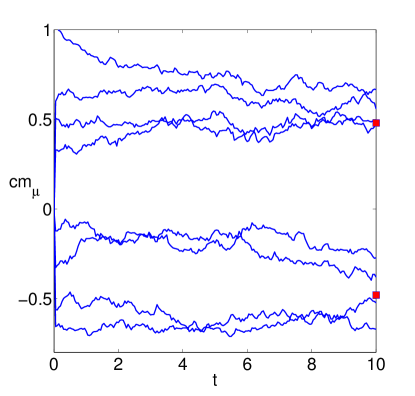
with a rescaled critical temperature T^c=T/csubscript^𝑇𝑐𝑇𝑐\hat{T}_{c}=T/c, due to the presence of dilution in the patterns. Each overlap approaches exponentially (one of) the non-zero (Gauge-symmetric) solutions of m=tanh(β^m)𝑚^𝛽𝑚m=\tanh(\hat{\beta}m) and the stable steady state of the system is given by 𝐦=m(1,,1)𝐦𝑚11{\bf m}=m(1,\ldots,1), for any temperature below criticality. This shows that the system is able to retrieve all the stored patterns in parallel and that the retrieval is symmetric. This behaviour is confirmed by Monte Carlo simulations, shown in figure 1, where the trajectories of the overlaps are seen to approach (up to finite size effects) the expected steady-states, represented by the symbols.
Refer to caption
Figure 1: Results of Monte Carlo simulations with N=104𝑁superscript104N=10^{4} spins at c=0.8𝑐0.8c=0.8, T^=T/c=0.6^𝑇𝑇𝑐0.6\hat{T}=T/c=0.6, γ=0.3𝛾0.3\gamma=0.3 and δ=0.25𝛿0.25\delta=0.25. We plot the overlaps mμsubscript𝑚𝜇m_{\mu} with different patterns 𝝃μsuperscript𝝃𝜇{\mbox{\boldmath$\xi$}}^{\mu}, drawn from (2), as a function of time t𝑡t. Red symbols represent the magnetisations in the steady state predicted by (46). Deviations from the predicted values are small and compatible with finite size effects 𝒪(Nγ)𝒪superscript𝑁𝛾\mathcal{O}(N^{-\gamma}).

Conversely, for any γδ𝛾𝛿\gamma\leq\delta, the dynamical equations (39) are coupled, meaning that there is an interference between patterns. This holds true even when the number of patterns is finite, i.e. for δ=γ=0𝛿𝛾0\delta=\gamma=0. In the sections below we will study the nature and stability of the stationary points of the dynamics for γδ𝛾𝛿\gamma\leq\delta and we show that despite the presence of pattern interference, the system is able to retrieve all stored patterns in parallel, although symmetric solutions will no longer be stable at all temperatures below criticality.

We will analyse, separately, the dynamics of the system for δ=0𝛿0\delta=0, i.e. the so-called low storage regime (Sec. 4), where the number of stored patterns is finite, and for δ>0𝛿0\delta>0, i.e. the so-called medium storage regime (Sec. 5), where the number of stored patterns is sub-linear in the system size.

4 Low Storage and Finite Dilution: γ=δ=0𝛾𝛿0\gamma=\delta=0

We have discussed above the case δ<γ𝛿𝛾\delta<\gamma, where overlaps of different patterns evolve independently and symmetric retrieval is stable for any temperature below criticality. Hence, the remainder of the paper is devoted to analyse the regime δγ𝛿𝛾\delta\geq\gamma, where, as explained is Sec. 3.2, a cross-talk between patterns appears. In this section we consider the case of finite number of patterns (δ=0𝛿0\delta=0), and finite dilution (γ=0𝛾0\gamma=0).

4.1 A toy model:P=2𝑃2P=2

Let us first illustrate the main features of the dynamics at low storage by considering the simple toy model with P=2𝑃2P=2 patterns. For γ=0𝛾0\gamma=0 and P=2𝑃2P=2 our dynamical equations (20) reduce to

tm1=f1(𝐦)=(1c)tanh(β^m1)+c2[tanh(β^(m1+m2))+tanh(β^(m1m2))]m1differential-ddifferential-d𝑡subscript𝑚1subscript𝑓1𝐦1𝑐^𝛽subscript𝑚1𝑐2delimited-[]^𝛽subscript𝑚1subscript𝑚2^𝛽subscript𝑚1subscript𝑚2subscript𝑚1\displaystyle\frac{\rmd}{\rmd t}m_{1}=f_{1}({\bf m})=(1-c)\tanh(\hat{\beta}m_{1})+\frac{c}{2}[\tanh(\hat{\beta}(m_{1}+m_{2}))+\tanh(\hat{\beta}(m_{1}-m_{2}))]-m_{1}
tm2=f2(𝐦)=(1c)tanh(β^m2)+c2[tanh(β^(m1+m2))tanh(β^(m1m2))]m2differential-ddifferential-d𝑡subscript𝑚2subscript𝑓2𝐦1𝑐^𝛽subscript𝑚2𝑐2delimited-[]^𝛽subscript𝑚1subscript𝑚2^𝛽subscript𝑚1subscript𝑚2subscript𝑚2\displaystyle\frac{\rmd}{\rmd t}m_{2}=f_{2}({\bf m})=(1-c)\tanh(\hat{\beta}m_{2})+\frac{c}{2}[\tanh(\hat{\beta}(m_{1}+m_{2}))-\tanh(\hat{\beta}(m_{1}-m_{2}))]-m_{2} (47)

Close to criticality, we have from (36), m1=m2=msubscript𝑚1subscript𝑚2𝑚m_{1}=m_{2}=m, with

m2=3ϵ3c𝐦213csuperscript𝑚23italic-ϵ3𝑐superscript𝐦213𝑐\displaystyle m^{2}=\frac{3\epsilon-3c{\bf m}^{2}}{1-3c} (48)

and 𝐦2=2m2superscript𝐦22superscript𝑚2{\bf m}^{2}=2m^{2}, yielding

m2=3ϵ1+3c.superscript𝑚23italic-ϵ13𝑐\displaystyle m^{2}=\frac{3\epsilon}{1+3c}. (49)

We analyse the stability of the symmetric mixtures studying the eigenvalues of the Jacobian (24) evaluated at the fixed point 𝐦=m(1,1)superscript𝐦𝑚11{\bf m}^{\star}=m(1,1). Solutions are linearly stable if the eigenvalues are negative. Due to the simple form of the matrix, eigenvalues are easily found as

λ1subscript𝜆1\displaystyle\lambda_{1} =\displaystyle= β^1(1c)β^tanh2(β^m)cβ^tanh2(2β^m)^𝛽11𝑐^𝛽superscript2^𝛽𝑚𝑐^𝛽superscript22^𝛽𝑚\displaystyle\hat{\beta}-1-(1-c)\hat{\beta}\tanh^{2}(\hat{\beta}m)-c\hat{\beta}\tanh^{2}(2\hat{\beta}m) (50)
λ2subscript𝜆2\displaystyle\lambda_{2} =\displaystyle= β^1(1c)β^tanh2(β^m).^𝛽11𝑐^𝛽superscript2^𝛽𝑚\displaystyle\hat{\beta}-1-(1-c)\hat{\beta}\tanh^{2}(\hat{\beta}m). (51)

We note that λ1<λ2subscript𝜆1subscript𝜆2\lambda_{1}<\lambda_{2}, hence the stability is given by the region where the largest eigenvalue λ2subscript𝜆2\lambda_{2} is negative. We can work out λ2subscript𝜆2\lambda_{2} analytically near TTcsimilar-to-or-equals𝑇subscript𝑇𝑐T\simeq T_{c} and T0similar-to-or-equals𝑇0T\simeq 0. Near the critical temperature, we expand (51) in powers of β^=cβ=1+ϵ^𝛽𝑐𝛽1italic-ϵ\hat{\beta}=c\beta=1+\epsilon and using (49) we find

λ2=2ϵ(13c)1+3c.subscript𝜆22italic-ϵ13𝑐13𝑐\displaystyle\lambda_{2}=-\frac{2\epsilon(1-3c)}{1+3c}. (52)

Hence, for TTcsimilar-to-or-equals𝑇subscript𝑇𝑐T\simeq T_{c} solutions are stable when c<1/3𝑐13c<1/3. In the opposite limit, T0𝑇0T\to 0, i.e. β𝛽\beta\to\infty, we have tanh2(βm)1superscript2𝛽𝑚1\tanh^{2}(\beta m)\to 1, and

λ2β^c1>0.similar-tosubscript𝜆2^𝛽𝑐10\displaystyle\lambda_{2}\sim\hat{\beta}c-1>0. (53)

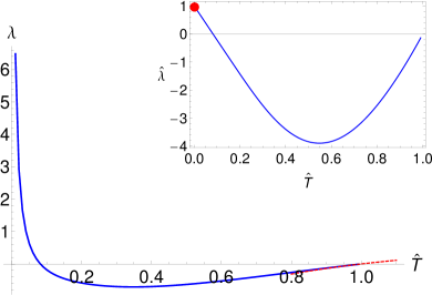
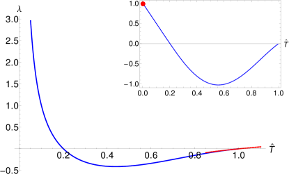
Hence, symmetric solutions are unstable at low temperature for any value of c>T𝑐𝑇c>\sqrt{T}. The full temperature-dependence of λ2subscript𝜆2\lambda_{2} can be obtained numerically and is shown in figure 2 for dilution c=0.2𝑐0.2c=0.2. The limits for temperature close to zero and to the critical point are in agreement with the theoretical predictions (52) and (53), shown in the graph and in the graph inset, as the dashed line and the symbol, respectively.
Refer to caption
Figure 2: Eigenvalue λ2subscript𝜆2\lambda_{2} as a function of the temperature T^^𝑇\hat{T}, for a fixed c=0.2𝑐0.2c=0.2. The red dashed line gives the theoretical prediction near the critical temperature (52). The figure in the inset shows agreement with (53), which gives λ2/(T^c)1subscript𝜆2^𝑇𝑐1\lambda_{2}/(\hat{T}c)\to 1 as T^0^𝑇0\hat{T}\to 0 (red marker).

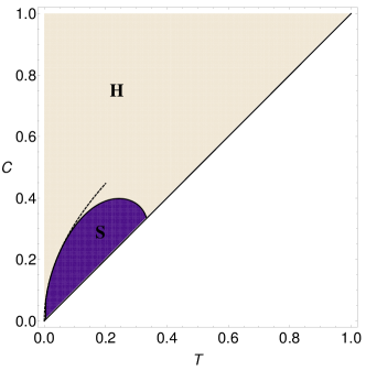
A contour plot of the critical line λ2=0subscript𝜆20\lambda_{2}=0 in the T𝑇T-c𝑐c place is shown in fig. 3. We highlight three regions: a paramagnetic region (𝐏𝐏{\bf P}) for T>Tc=c𝑇subscript𝑇𝑐𝑐T>T_{c}=c where the only solution is 𝐦=0𝐦0{\bf m}=0; a region (𝐒𝐒{\bf S}) for T<c𝑇𝑐T<c and for c<1/3𝑐13c<1/3 where symmetric solutions are stable; finally a region (𝐇𝐇{\bf H}) where 𝐦0𝐦0{\bf m}\neq 0 and symmetric mixtures are unstable, so that a new class of asymmetric solutions takes over, the so-called hierarchical solutions.
Refer to caption
Figure 3: Phase diagram in the parameter space (T,c)𝑇𝑐(T,c) for the case δ=γ=0𝛿𝛾0\delta=\gamma=0 (P=2𝑃2P=2). The (S) area represents the region where the symmetric mixtures are stable; the (H) region is characterised by hierarchical states, while the paramagnetic state (P) is stable for T>Tc=c𝑇subscript𝑇𝑐𝑐T>T_{c}=c. The (S) region is obtained as the contour plot of the equation λ2=0subscript𝜆20\lambda_{2}=0 solved numerically together with equations (47) at stationarity. The approach to zero is consistent with c=T𝑐𝑇c=\sqrt{T} predicted by the theory (dashed line).

For T0𝑇0T\to 0 these take the form 𝐦=(1,1c)𝐦11𝑐{\bf m}=(1,1-c), which is the steady state of the system (47) for β𝛽\beta\to\infty. Calculating the eigenvalues λ1,λ2subscript𝜆1subscript𝜆2\lambda_{1},\lambda_{2} of the stability matrix (24) evaluated at 𝐦=(1,1c)superscript𝐦11𝑐{\bf m}^{\star}=(1,1-c), we have λ1,λ21subscript𝜆1subscript𝜆21\lambda_{1},\lambda_{2}\to-1 as β𝛽\beta\to\infty, so 𝐦=(1,1c)𝐦11𝑐{\bf m}=(1,1-c) is an attractor at low temperature.

This behaviour is confirmed by Monte Carlo simulations and by the phase portrait of the dynamical system (47), both shown in fig. 4. One can see that phase curves for T^=1.25^𝑇1.25\hat{T}=1.25, i.e. T>Tc𝑇subscript𝑇𝑐T>T_{c}, evolve to the steady state 𝐦=0𝐦0{\bf m}=0; phase curves at temperature T^=0.8^𝑇0.8\hat{T}=0.8 and c=0.25𝑐0.25c=0.25, (inside the (S) region), evolves to symmetric mixtures (where m1=m2subscript𝑚1subscript𝑚2m_{1}=m_{2}); at smaller temperature, T^=0.01^𝑇0.01\hat{T}=0.01, and c=0.5𝑐0.5c=0.5 (inside the (H) region), symmetric states become unstable with phase velocities pointing away from them, and non-symmetric stable steady states (with m1m2subscript𝑚1subscript𝑚2m_{1}\neq m_{2}) appear. At T^=0.01^𝑇0.01\hat{T}=0.01, the system evolves towards the low temperature hierarchical state 𝐦=(1,1c)𝐦11𝑐{\bf m}=(1,1-c). Results are in agreement with equilibrium analysis and simulations [1, 10, 6].

Refer to caption
Refer to caption
Refer to caption
Refer to caption
Refer to caption
Refer to caption
Figure 4: Left panels: Phase portraits of the dynamical system (47) in different regimes of noise T𝑇T and dilution c𝑐c; red lines represent the null-clines, and stationary states are at the intersections of null-clines. Right panels: Monte-Carlo simulations with N=104𝑁superscript104N=10^{4} spins, with T𝑇T and c𝑐c as in the left panels; red markers represent the stationary states of the dynamical system. From top to bottom: c=0.4,T^=1.25formulae-sequence𝑐0.4^𝑇1.25c=0.4,\hat{T}=1.25; c=0.25,T^=0.8formulae-sequence𝑐0.25^𝑇0.8c=0.25,\hat{T}=0.8; c=0.5𝑐0.5c=0.5, T^=0.01^𝑇0.01\hat{T}=0.01: in the latter regime, stationary states are given by 𝐦=(1,1c)𝐦11𝑐{\bf m}=(1,1-c), as expected at low temperature.

4.2 Generalisation to P>2𝑃2P>2 patterns

Generalising to P𝑃P patterns, and assuming we have, close to criticality, 𝐦=m(1,,1,0,,0)𝐦𝑚1100{\bf m}=m(1,\ldots,1,0,\ldots,0) with 𝐦2=nm2superscript𝐦2𝑛superscript𝑚2{\bf m}^{2}=nm^{2}, we get from (36)

m2=3ϵ13c+3cn,superscript𝑚23italic-ϵ13𝑐3𝑐𝑛\displaystyle m^{2}=\frac{3\epsilon}{1-3c+3cn}, (54)

that coincides with (49) for P=n=2𝑃𝑛2P=n=2. To study the stability of symmetric mixtures, we evaluate the Jacobian (24) at the steady state 𝐦=m(1,,1,0,,0)superscript𝐦𝑚1100{\bf m}^{\star}=m(1,\dots,1,0,\dots,0). Diagonal elements are given by (26), (27) where, for symmetric states,

qμsubscript𝑞𝜇\displaystyle q_{\mu} =\displaystyle= (tanh2(β^m(1+νμnξν))𝝃\displaystyle\langle(\tanh^{2}(\hat{\beta}m(1+\sum_{\nu\neq\mu}^{n}\xi^{\nu}))\rangle_{{\mbox{\boldmath$\xi$}}} (55)
q𝑞\displaystyle q =\displaystyle= (tanh2(β^mν=1nξν)𝝃\displaystyle\langle(\tanh^{2}(\hat{\beta}m\sum_{\nu=1}^{n}\xi^{\nu})\rangle_{{\mbox{\boldmath$\xi$}}} (56)

whereas off-diagonal elements are, for γ=0𝛾0\gamma=0,

Aμνsubscript𝐴𝜇𝜈\displaystyle A_{\mu\nu} =\displaystyle= β^Q,forμ,νn^𝛽𝑄for𝜇𝜈𝑛\displaystyle-\hat{\beta}Q,\quad\quad{\rm for\leavevmode\nobreak\ }\mu,\nu\leq n
Aμνsubscript𝐴𝜇𝜈\displaystyle A_{\mu\nu} =\displaystyle= 0,otherwise0otherwise\displaystyle 0,\quad\quad\quad\quad{\rm otherwise} (57)

with

Q=1c(ξμξνtanh2(β^mν=1nξν)𝝃.\displaystyle Q=\frac{1}{c}\langle(\xi^{\mu}\xi^{\nu}\tanh^{2}(\hat{\beta}m\sum_{\nu=1}^{n}\xi^{\nu})\rangle_{{\mbox{\boldmath$\xi$}}}. (58)

Due to the symmetry of the problem, we have three distinct eigenspaces, with qμ=q1μsubscript𝑞𝜇subscript𝑞1for-all𝜇q_{\mu}=q_{1}\leavevmode\nobreak\ \forall\leavevmode\nobreak\ \mu:

EigenspacesEigenspaces\displaystyle{\rm Eigenspaces}\quad\quad EigenvaluesEigenvalues\displaystyle{\rm Eigenvalues}
𝐱=(1,,1,0,,0)𝐱1100\displaystyle{\bf x}=(1,\ldots,1,0,\ldots,0)\quad\quad λ1=β^(1q1)1β^(n1)Qsubscript𝜆1^𝛽1subscript𝑞11^𝛽𝑛1𝑄\displaystyle\lambda_{1}=\hat{\beta}(1-q_{1})-1-\hat{\beta}(n-1)Q
𝐱=(x1,,xn,0,,0),μxμ=0𝐱subscript𝑥1subscript𝑥𝑛00subscript𝜇subscript𝑥𝜇0\displaystyle{\bf x}=(x_{1},\ldots,x_{n},0,\ldots,0),\quad{\mbox{$\sum_{\mu}x_{\mu}=0$}}\quad\quad λ2=β^(1q1)1+β^Qsubscript𝜆2^𝛽1subscript𝑞11^𝛽𝑄\displaystyle\lambda_{2}=\hat{\beta}(1-q_{1})-1+\hat{\beta}Q
𝐱=(0,,0,nn+1,,xP)𝐱00subscript𝑛𝑛1subscript𝑥𝑃\displaystyle{\bf x}=(0,\ldots,0,n_{n+1},\ldots,x_{P})\quad\quad λ3=β^(1q)1subscript𝜆3^𝛽1𝑞1\displaystyle\lambda_{3}=\hat{\beta}(1-q)-1

Near TTcsimilar-to-or-equals𝑇subscript𝑇𝑐T\simeq T_{c} we Taylor expand q1,q,Qsubscript𝑞1𝑞𝑄q_{1},q,Q in powers of t=β^1𝑡^𝛽1t=\hat{\beta}-1, obtaining respectively:

q1=3ϵ+3(n1)cϵ13c+3cnsubscript𝑞13italic-ϵ3𝑛1𝑐italic-ϵ13𝑐3𝑐𝑛\displaystyle q_{1}=\frac{3\epsilon+3(n-1)c\epsilon}{1-3c+3cn} (59)
q=3ncϵ13c+3cn𝑞3𝑛𝑐italic-ϵ13𝑐3𝑐𝑛\displaystyle q=\frac{3nc\epsilon}{1-3c+3cn} (60)
Q=6ϵc13c+3cn.𝑄6italic-ϵ𝑐13𝑐3𝑐𝑛\displaystyle Q=\frac{6\epsilon c}{1-3c+3cn}. (61)

Hence, eigenvalues near the critical temperature are given by

λ1=2ϵ+6cϵ6cϵn13c+3cnsubscript𝜆12italic-ϵ6𝑐italic-ϵ6𝑐italic-ϵ𝑛13𝑐3𝑐𝑛\displaystyle\lambda_{1}=-\frac{-2\epsilon+6c\epsilon-6c\epsilon n}{1-3c+3cn} (62)
λ2=2ϵ+6cϵ13c+3cnsubscript𝜆22italic-ϵ6𝑐italic-ϵ13𝑐3𝑐𝑛\displaystyle\lambda_{2}=\frac{-2\epsilon+6c\epsilon}{1-3c+3cn} (63)
λ3=ϵ3cϵ13c+3cn.subscript𝜆3italic-ϵ3𝑐italic-ϵ13𝑐3𝑐𝑛\displaystyle\lambda_{3}=\frac{\epsilon-3c\epsilon}{1-3c+3cn}. (64)

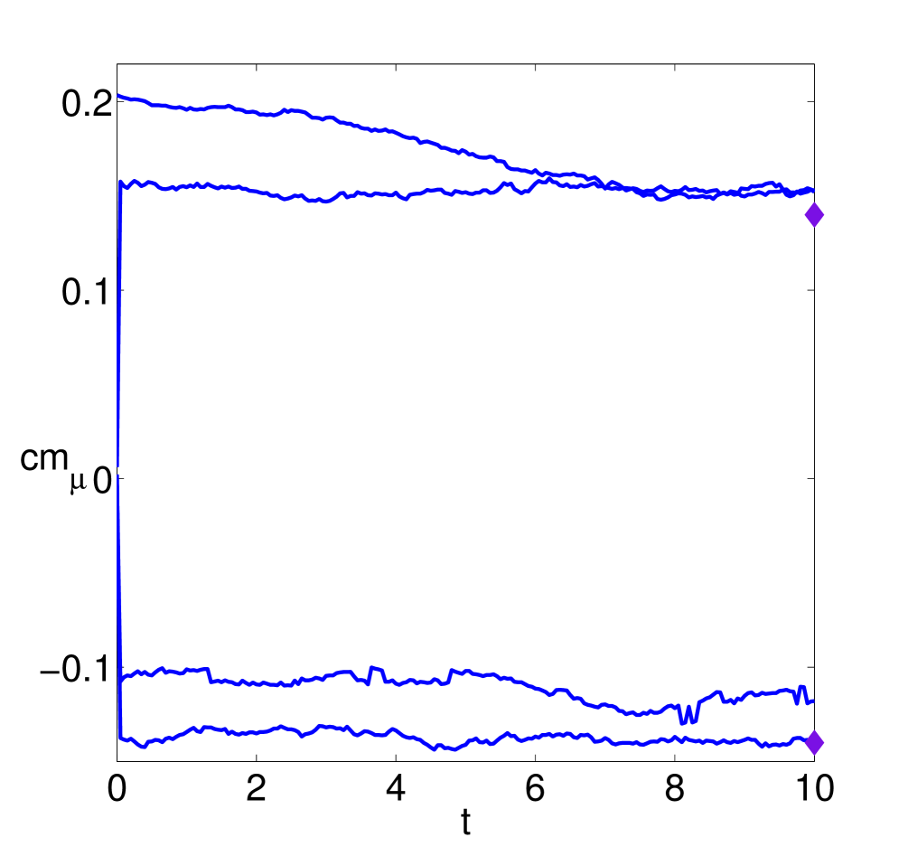
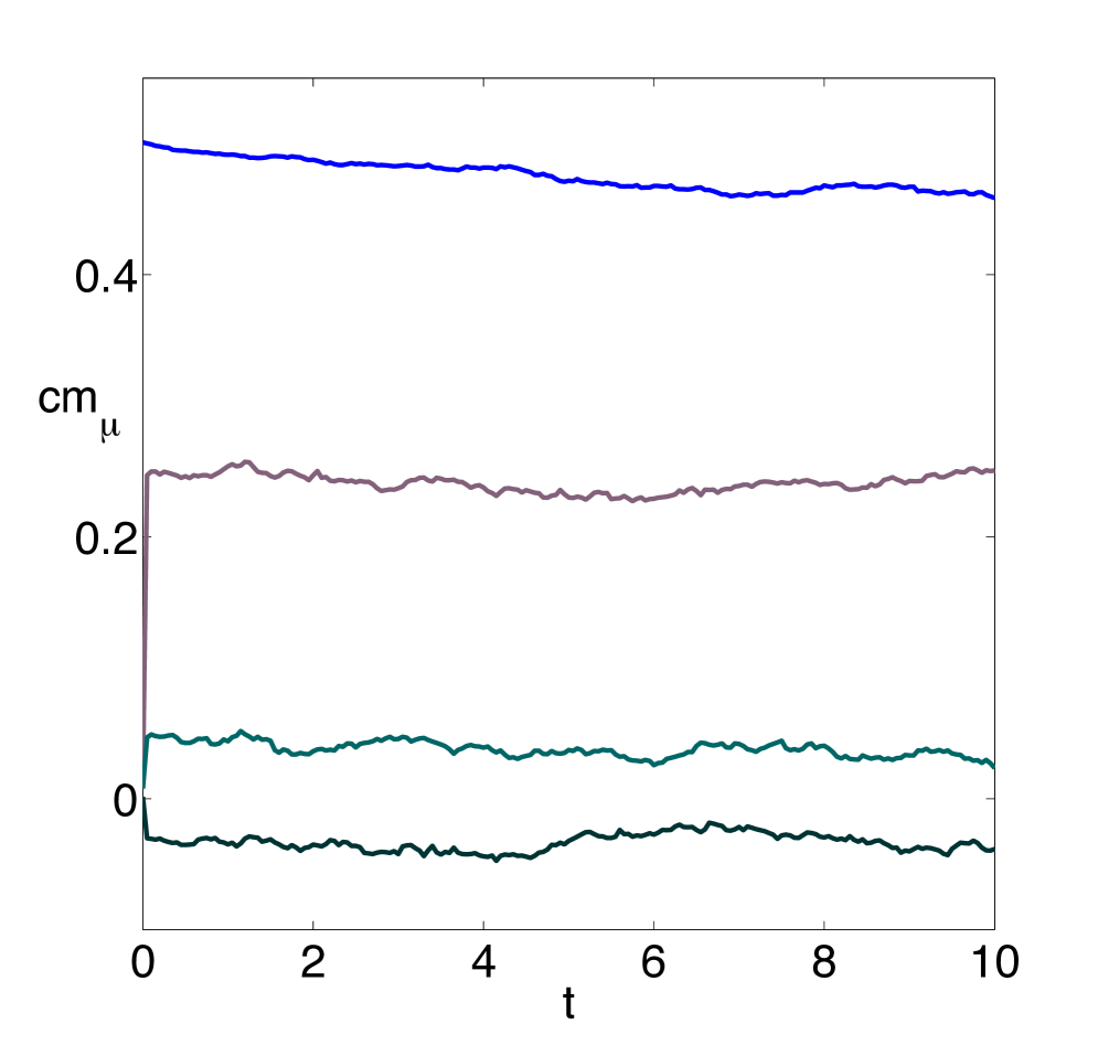
We note that λ1<0subscript𝜆10\lambda_{1}<0 for any c𝑐c, and, as in the case P=2𝑃2P=2, λ2<0subscript𝜆20\lambda_{2}<0 for c<1/3𝑐13c<1/3. On the other hand, λ3<0subscript𝜆30\lambda_{3}<0 for c>1/3𝑐13c>1/3. Since the eigenvalue λ3subscript𝜆3\lambda_{3} only comes into play for P>n𝑃𝑛P>n, symmetric mixtures 𝐦=m(1,,1)𝐦𝑚11{\bf m}=m(1,\dots,1) , where all patterns are recalled, i.e. with n=P𝑛𝑃n=P, are stable for any c<1/3𝑐13c<1/3, near criticality. In contrast, there is no region of the phase space where mixtures of the form 𝐦=m(1,,1,0,,0)𝐦𝑚1100{\bf m}=m(1,\dots,1,0,\dots,0), in which a number of patterns is not recalled, is stable. Results are confirmed by Monte-Carlo simulations shown in fig. 5. Interestingly, the stability threshold c<1/3𝑐13c<1/3 near Tcsubscript𝑇𝑐T_{c} is independent of the number of patterns P𝑃P. However we note that at other temperatures, the eigenvalues and their stability will in general depend on the number of patterns involved [10].
Refer to caption
Refer to caption
Figure 5: Simulations with N=104𝑁superscript104N=10^{4} spins and P=4𝑃4P=4 patterns of mμsubscript𝑚𝜇m_{\mu} as a function of time. Left Panel: Symmetric solutions for T^=0.5^𝑇0.5\hat{T}=0.5, c=0.2𝑐0.2c=0.2. The markers represent the amplitude of the symmetric mixtures evaluated solving the self-consistency equation for P=4𝑃4P=4 (67). Right Panel: hierarchical retrieval for c=0.5𝑐0.5c=0.5 and T^=0.4.^𝑇0.4\hat{T}=0.4.

At low temperature, symmetric mixtures become unstable. In order to show this, it is convenient to introduce the noise distribution

Pn(z)subscript𝑃𝑛𝑧\displaystyle P_{n}(z) =\displaystyle= δ(zν=1nξν)𝝃=ππω2πωz^ν=1nωξν𝝃subscriptdelimited-⟨⟩𝛿𝑧superscriptsubscript𝜈1𝑛superscript𝜉𝜈𝝃superscriptsubscript𝜋𝜋differential-d𝜔2𝜋superscript𝜔^𝑧superscriptsubscriptproduct𝜈1𝑛subscriptdelimited-⟨⟩superscript𝜔superscript𝜉𝜈𝝃\displaystyle{\langle}\delta(z-\sum_{\nu=1}^{n}\xi^{\nu}){\rangle}_{\mbox{\boldmath$\xi$}}=\int_{-\pi}^{\pi}\frac{\rmd\omega}{2\pi}\rme^{-\rmi\omega\hat{z}}\prod_{\nu=1}^{n}\langle\rme^{\rmi\omega\xi^{\nu}}\rangle_{{\mbox{\boldmath$\xi$}}} (65)
=\displaystyle= ππω2πωz[1+c(cosω1)]nsuperscriptsubscript𝜋𝜋differential-d𝜔2𝜋superscript𝜔𝑧superscriptdelimited-[]1𝑐𝜔1𝑛\displaystyle\int_{-\pi}^{\pi}\frac{\rmd\omega}{2\pi}\rme^{-\rmi\omega z}[1+c(\cos\omega-1)]^{n}

where n𝑛n is the number of retrieved patterns. We can express q1subscript𝑞1q_{1} and q𝑞q, as given in (28), (29), in terms of (65):

q1subscript𝑞1\displaystyle q_{1} =\displaystyle= zPn1(z)tanh2(β^m(1+z))subscript𝑧subscript𝑃𝑛1𝑧superscript2^𝛽𝑚1𝑧\displaystyle\sum_{z}P_{n-1}(z)\tanh^{2}(\hat{\beta}m(1+z))
q𝑞\displaystyle q =\displaystyle= zPn(z)tanh2(β^mz)subscript𝑧subscript𝑃𝑛𝑧superscript2^𝛽𝑚𝑧\displaystyle\sum_{z}P_{n}(z)\tanh^{2}(\hat{\beta}mz) (66)

and the self-consistency equation for the amplitude m𝑚m of the symmetric mixtures m𝑚m becomes

m=zPn1(z)tanh(β^m(1+z)).𝑚subscript𝑧subscript𝑃𝑛1𝑧^𝛽𝑚1𝑧\displaystyle m=\sum_{z}P_{n-1}(z)\tanh(\hat{\beta}m(1+z)). (67)

It is easy to see that Pn(z)subscript𝑃𝑛𝑧P_{n}(z) satisfies a useful recursion relation

Pn(z)=(1c)Pn1(z)+cPn1(z+1)+Pn1(z1)2subscript𝑃𝑛𝑧1𝑐subscript𝑃𝑛1𝑧𝑐subscript𝑃𝑛1𝑧1subscript𝑃𝑛1𝑧12P_{n}(z)=(1-c)P_{n-1}(z)+c\frac{P_{n-1}(z+1)+P_{n-1}(z-1)}{2} (68)

which represents a discrete-time lazy, symmetric random walker, taking right and left unit steps along the z𝑧z-axis with equal probabilities c/2𝑐2c/2. All the Pnsubscript𝑃𝑛P_{n}’s in the hierarchy can then be determined from knowledge of P0(z)δ(z)subscript𝑃0𝑧𝛿𝑧P_{0}(z)\equiv\delta(z). The random walker is lazy for c<1𝑐1c<1 because at each iteration n𝑛n it has a finite probability to take no step. When β𝛽\beta\to\infty, q11Pn1(1)subscript𝑞11subscript𝑃𝑛11q_{1}\to 1-P_{n-1}(-1), q1Pn(0)𝑞1subscript𝑃𝑛0q\to 1-P_{n}(0) and Q0𝑄0Q\to 0, hence

λ1,2β^Pn1(1)1subscript𝜆12^𝛽subscript𝑃𝑛111\displaystyle\lambda_{1,2}\to\hat{\beta}P_{n-1}(1)-1 (69)
λ3β^Pn(0)1subscript𝜆3^𝛽subscript𝑃𝑛01\displaystyle\lambda_{3}\to\hat{\beta}P_{n}(0)-1 (70)

where we used Pn(z)=Pn(z)subscript𝑃𝑛𝑧subscript𝑃𝑛𝑧P_{n}(z)=P_{n}(-z). We note that for c<1𝑐1c<1, we have a non-zero probability Pn(0)>0subscript𝑃𝑛00P_{n}(0)>0 for the walker to be at the origin for any finite time n0𝑛0n\geq 0, hence symmetric mixtures are unstable for any value of n𝑛n at low temperature. In contrast, c=1𝑐1c=1 introduces a periodicity in the return times of the walker, so that Pn(0)=0subscript𝑃𝑛00P_{n}(0)=0 for n𝑛n odd and Pn(1)=0subscript𝑃𝑛10P_{n}(1)=0 for n𝑛n even, so that for n𝑛n odd (even) all eigenvalues are negative (positive), in agreement with the standard (i.e. undiluted) Hopfield model [3], where, at zero temperature, all odd mixtures are attractors and all even mixtures are unstable. In particular, for n=1𝑛1n=1, λ1,2=1subscript𝜆121\lambda_{1,2}=-1 and from (68)

P1(z)subscript𝑃1𝑧\displaystyle P_{1}(z) =\displaystyle= (1c)δ(z)+cδ(z+1)+δ(z1)21𝑐𝛿𝑧𝑐𝛿𝑧1𝛿𝑧12\displaystyle(1-c)\delta(z)+c\frac{\delta(z+1)+\delta(z-1)}{2} (71)

so λ3=β^(1c)1subscript𝜆3^𝛽1𝑐1\lambda_{3}=\hat{\beta}(1-c)-1. Hence, the so-called pure state, where the system recalls only one pattern, is stable at low temperature only for the undiluted case c=1𝑐1c=1, but it is unstable for any c<1𝑐1c<1.

In [1, 10], an ansatz was made for the form of the magnetisation vector in the hierarchical state at T=0𝑇0T=0,

mμ=(1c)μ1μ=1,,nformulae-sequencesubscript𝑚𝜇superscript1𝑐𝜇1𝜇1𝑛\displaystyle m_{\mu}=(1-c)^{\mu-1}\quad\quad\mu=1,\ldots,n (72)

where nP𝑛𝑃n\leq P is the number of condensed patterns and mμ=0μ>nsubscript𝑚𝜇0for-all𝜇𝑛m_{\mu}=0\leavevmode\nobreak\ \forall\leavevmode\nobreak\ \mu>n. We shall denote briefly this state as 𝐦Hsubscript𝐦𝐻{\bf m}_{H}. We note that (72), with n=P𝑛𝑃n=P, are indeed fixed points of (47) for β𝛽\beta\to\infty and P=2𝑃2P=2, and for larger P𝑃P, they solve self-consistently (21) for β𝛽\beta\to\infty for wide regions of the dilution parameter c𝑐c. The stability of this solution is given by the eigenvalues of the stability matrix (24) evaluated at 𝐦=𝐦Hsuperscript𝐦subscript𝐦𝐻{\bf m}^{\star}={\bf m}_{H}. The matrix is again diagonal in the limit β𝛽\beta\to\infty, with elements given in (26), (27) and

qμsubscript𝑞𝜇\displaystyle q_{\mu} =\displaystyle= (tanh2(β^(mμ+νμnξνmν))𝝃\displaystyle\langle(\tanh^{2}(\hat{\beta}(m_{\mu}+\sum_{\nu\neq\mu}^{n}\xi^{\nu}m_{\nu}))\rangle_{{\mbox{\boldmath$\xi$}}} (73)
q𝑞\displaystyle q =\displaystyle= (tanh2(β^ν=1nξνmμ)𝝃.\displaystyle\langle(\tanh^{2}(\hat{\beta}\sum_{\nu=1}^{n}\xi^{\nu}m_{\mu})\rangle_{{\mbox{\boldmath$\xi$}}}. (74)

Upon introducing Pμ(z)=δ(zνμnξνmν)P_{\mu}(z)={\langle}\delta(z-\sum_{\nu\neq\mu}^{n}\xi^{\nu}m_{\nu}) and P(z)=δ(zν=1nξνmν)P(z)={\langle}\delta(z-\sum_{\nu=1}^{n}\xi^{\nu}m_{\nu}), we can rewrite these as

qμsubscript𝑞𝜇\displaystyle q_{\mu} =\displaystyle= ztanh2(β^(mμ+z)Pμ(z)\displaystyle\int\rmd z\tanh^{2}(\hat{\beta}(m_{\mu}+z)P_{\mu}(z) (75)
q𝑞\displaystyle q =\displaystyle= ztanh2(β^z)P(z)differential-d𝑧superscript2^𝛽𝑧𝑃𝑧\displaystyle\int\rmd z\tanh^{2}(\hat{\beta}z)P(z) (76)

For β𝛽\beta\to\infty, we have

Aμμ=β^Pμ(mμ)1,subscript𝐴𝜇𝜇^𝛽subscript𝑃𝜇subscript𝑚𝜇1\displaystyle A_{\mu\mu}=\hat{\beta}P_{\mu}(-m_{\mu})-1, forμnfor𝜇𝑛\displaystyle\quad{\rm for\leavevmode\nobreak\ }\mu\leq n (77)
Aμμ=β^P(0)1,subscript𝐴𝜇𝜇^𝛽𝑃01\displaystyle A_{\mu\mu}=\hat{\beta}P(0)-1, forμ>nfor𝜇𝑛\displaystyle\quad{\rm for\leavevmode\nobreak\ }\mu>n (78)

Working out

Pμ(z)=ω2πωzνμnωξνmν𝝃=ω2πωzνμn[1+c(cos(ωmν)1)]subscript𝑃𝜇𝑧superscriptsubscriptdifferential-d𝜔2𝜋superscript𝜔𝑧superscriptsubscriptproduct𝜈𝜇𝑛subscriptdelimited-⟨⟩superscript𝜔superscript𝜉𝜈subscript𝑚𝜈𝝃superscriptsubscriptdifferential-d𝜔2𝜋superscript𝜔𝑧superscriptsubscriptproduct𝜈𝜇𝑛delimited-[]1𝑐𝜔subscript𝑚𝜈1\displaystyle P_{\mu}(z)=\int_{-\infty}^{\infty}\frac{\rmd\omega}{2\pi}\rme^{-\rmi\omega z}\prod_{\nu\neq\mu}^{n}\langle\rme^{\rmi\omega\xi^{\nu}m_{\nu}}\rangle_{{\mbox{\boldmath$\xi$}}}=\int_{-\infty}^{\infty}\frac{\rmd\omega}{2\pi}\rme^{-\rmi\omega z}\prod_{\nu\neq\mu}^{n}[1+c(\cos(\omega m_{\nu})-1)] (79)

and

P(z)=ω2πiωzν=1n[1+c(cos(ωmν)1)]𝑃𝑧superscriptsubscriptdifferential-d𝜔2𝜋superscript𝑖𝜔𝑧superscriptsubscriptproduct𝜈1𝑛delimited-[]1𝑐𝜔subscript𝑚𝜈1P(z)=\int_{-\infty}^{\infty}\frac{\rmd\omega}{2\pi}\,\rme^{-i\omega z}\prod_{\nu=1}^{n}[1+c(\cos(\omega m_{\nu})-1)] (80)

again, we can relate P(z)𝑃𝑧P(z) and Pμ(z)subscript𝑃𝜇𝑧P_{\mu}(z), μfor-all𝜇\forall\leavevmode\nobreak\ \mu, as follows

P(z)=(1c)Pμ(z)+cPμ(z+mμ)+Pμ(zmμ)2𝑃𝑧1𝑐subscript𝑃𝜇𝑧𝑐subscript𝑃𝜇𝑧subscript𝑚𝜇subscript𝑃𝜇𝑧subscript𝑚𝜇2P(z)=(1-c)P_{\mu}(z)+c\frac{P_{\mu}(z+m_{\mu})+P_{\mu}(z-m_{\mu})}{2} (81)

Setting z=0𝑧0z=0 in the above, we have

P(0)=(1c)Pμ(0)+cPμ(mμ)𝑃01𝑐subscript𝑃𝜇0𝑐subscript𝑃𝜇subscript𝑚𝜇P(0)=(1-c)P_{\mu}(0)+cP_{\mu}(m_{\mu}) (82)

hence stability along the directions μ=n+1,,P𝜇𝑛1𝑃\mu=n+1,\ldots,P, which requires P(0)=0𝑃00P(0)=0, implies Pμ(mμ)=Pμ(0)=0μsubscript𝑃𝜇subscript𝑚𝜇subscript𝑃𝜇00for-all𝜇P_{\mu}(m_{\mu})=P_{\mu}(0)=0\leavevmode\nobreak\ \forall\leavevmode\nobreak\ \mu i.e. stability along the directions μ=1,n𝜇1𝑛\mu=1\ldots,n, since for 0<c<10𝑐10<c<1 the two terms on the RHS are both non-negative. However, P(0)=δ(νξνmν)𝑃0delimited-⟨⟩𝛿subscript𝜈superscript𝜉𝜈subscript𝑚𝜈P(0)={\langle}\delta(\sum_{\nu}\xi^{\nu}m_{\nu}){\rangle} is bounded from below by the probability of drawing 𝝃=𝟎𝝃0{\mbox{\boldmath$\xi$}}={\bf 0}, i.e. P(0)(1c)n>0𝑃0superscript1𝑐𝑛0P(0)\geq(1-c)^{n}>0, so hierarchic mixtures can only be stable for P=n𝑃𝑛P=n. The condition for their stability is Pμ(mμ)=0μPsubscript𝑃𝜇subscript𝑚𝜇0for-all𝜇𝑃P_{\mu}(m_{\mu})=0\leavevmode\nobreak\ \forall\leavevmode\nobreak\ \mu\leq P. It is easy to see that this condition is satisfied for P=2𝑃2P=2, where (81) yields P1(1)=c[δ(c)+δ(2c)]/2subscript𝑃11𝑐delimited-[]𝛿𝑐𝛿2𝑐2P_{1}(1)=c[\delta(c)+\delta(2-c)]/2 and P2(1c)=(1c)δ(1c)+c[δ(c)+δ(2c)]/2subscript𝑃21𝑐1𝑐𝛿1𝑐𝑐delimited-[]𝛿𝑐𝛿2𝑐2P_{2}(1-c)=(1-c)\delta(1-c)+c[\delta(c)+\delta(2-c)]/2, both vanishing for any c(0,1)𝑐01c\in(0,1).

5 Extreme dilution and medium storage regime

Next we analyse the dynamical behaviour of the system in the medium load regime (i.e. δ>0𝛿0\delta>0), where the number of patterns scales sub-linearly in the system size, when patterns are extremely diluted (i.e. γ>0𝛾0\gamma>0).

5.1 Cross-talk effect for δ=γ𝛿𝛾\delta=\gamma

In this section we study the case δ=γ𝛿𝛾\delta=\gamma. We have shown in Sec. 3 that the first class of stationary states to bifurcate away from 𝐦=0𝐦0{\bf m}=0 below criticality, are the symmetric mixtures 𝐦=m(1,,1,0,,0)𝐦𝑚1100{\bf m}=m(1,\dots,1,0,\dots,0), with 𝐦2=nm2superscript𝐦2𝑛superscript𝑚2{\bf m}^{2}=nm^{2}, where n𝑛n is the number of retrieved components.
For δ=γ>0𝛿𝛾0\delta=\gamma>0, we assume that n𝑛n is a fraction of the total number of patterns P=αNγ𝑃𝛼superscript𝑁𝛾P=\alpha N^{\gamma}, hence we set n=ϕNγ𝑛italic-ϕsuperscript𝑁𝛾n=\phi N^{\gamma}, with 0ϕα0italic-ϕ𝛼0\leq\phi\leq\alpha. Using 𝐦2=ϕNγm2superscript𝐦2italic-ϕsuperscript𝑁𝛾superscript𝑚2{\bf m}^{2}=\phi N^{\gamma}m^{2} in (35), we have

m23ϵ1+3cϕsimilar-to-or-equalssuperscript𝑚23italic-ϵ13𝑐italic-ϕ\displaystyle m^{2}\simeq\frac{3\epsilon}{1+3c\phi} (83)

Again, to analyse the stability of symmetric mixtures, we look at the eigenvalues of the Jacobian (24) evaluated at 𝐦=m(1,,1,0,,0)𝐦𝑚1100{\bf m}=m(1,\dots,1,0,\dots,0). Its elements are given by (26), (27) and (30), where, for symmetric states, qμ=q1μsubscript𝑞𝜇subscript𝑞1for-all𝜇q_{\mu}=q_{1}\leavevmode\nobreak\ \forall\leavevmode\nobreak\ \mu and

q1=tanh2(β^m(1+νμϕNγξν)𝝃,\displaystyle q_{1}=\langle\tanh^{2}(\hat{\beta}m(1+\sum_{\nu\neq\mu}^{\phi N^{\gamma}}\xi^{\nu})\rangle_{{\mbox{\boldmath$\xi$}}}, (84)
q=tanh2(β^mνμϕNγξν)𝝃𝑞subscriptdelimited-⟨⟩superscript2^𝛽𝑚superscriptsubscript𝜈𝜇italic-ϕsuperscript𝑁𝛾superscript𝜉𝜈𝝃\displaystyle q=\langle\tanh^{2}(\hat{\beta}m\sum_{\nu\neq\mu}^{\phi N^{\gamma}}\xi^{\nu})\rangle_{{\mbox{\boldmath$\xi$}}} (85)

As before, it is convenient to consider the distribution Pϕ(z)=δ(zμνϕNγξν)𝝃subscript𝑃italic-ϕ𝑧subscriptdelimited-⟨⟩𝛿𝑧superscriptsubscript𝜇𝜈italic-ϕsuperscript𝑁𝛾superscript𝜉𝜈𝝃P_{\phi}(z)=\langle\delta(z-\sum_{\mu\neq\nu}^{\phi N^{\gamma}}\xi^{\nu})\rangle_{{\mbox{\boldmath$\xi$}}}. In the thermodynamic limit it can be written as

Pϕ(z)=ππω2πωz+cϕ(cosω1)=ϕcIz(ϕc)subscript𝑃italic-ϕ𝑧superscriptsubscript𝜋𝜋differential-d𝜔2𝜋superscript𝜔𝑧𝑐italic-ϕ𝜔1superscriptitalic-ϕ𝑐subscript𝐼𝑧italic-ϕ𝑐\displaystyle P_{\phi}(z)=\int_{-\pi}^{\pi}\frac{\rmd\omega}{2\pi}\rme^{-\rmi\omega z+c\phi(\cos\omega-1)}=\rme^{-\phi c}I_{z}(\phi c) (86)

where Iz(ϕc)subscript𝐼𝑧italic-ϕ𝑐I_{z}(\phi c) is the modified Bessel function of the first kind [14]. Clearly, Pϕ(z)=Pϕ(z)subscript𝑃italic-ϕ𝑧subscript𝑃italic-ϕ𝑧P_{\phi}(z)=P_{\phi}(-z), and due to the property of the Bessel functions,

dIn(t)dt=12[In1(t)+In+1(t)],𝑑subscript𝐼𝑛𝑡𝑑𝑡12delimited-[]subscript𝐼𝑛1𝑡subscript𝐼𝑛1𝑡\frac{dI_{n}(t)}{dt}=\frac{1}{2}[I_{n-1}(t)+I_{n+1}(t)],

Pϕ(z)subscript𝑃italic-ϕ𝑧P_{\phi}(z) evolves according to

dPϕ(z)dϕ=c2[Pϕ(z1)+Pϕ(z+1)2Pϕ(z)]𝑑subscript𝑃italic-ϕ𝑧𝑑italic-ϕ𝑐2delimited-[]subscript𝑃italic-ϕ𝑧1subscript𝑃italic-ϕ𝑧12subscript𝑃italic-ϕ𝑧\frac{dP_{\phi}(z)}{d\phi}=\frac{c}{2}[P_{\phi}(z-1)+P_{\phi}(z+1)-2P_{\phi}(z)]

which describes a continuous-time symmetric random walker taking unit steps along the z𝑧z-axis with rate c/2𝑐2c/2, as ϕitalic-ϕ\phi increases. We can rewrite q1subscript𝑞1q_{1} and q𝑞q in terms of Pϕ(z)subscript𝑃italic-ϕ𝑧P_{\phi}(z), as:

q1subscript𝑞1\displaystyle q_{1} =\displaystyle= zPϕ(z)tanh2(β^m(1+z))subscript𝑧subscript𝑃italic-ϕ𝑧superscript2^𝛽𝑚1𝑧\displaystyle\sum_{z}P_{\phi}(z)\tanh^{2}(\hat{\beta}m(1+z)) (87)
q𝑞\displaystyle q =\displaystyle= zPϕ(z)tanh2(β^mz)subscript𝑧subscript𝑃italic-ϕ𝑧superscript2^𝛽𝑚𝑧\displaystyle\sum_{z}P_{\phi}(z)\tanh^{2}(\hat{\beta}mz) (88)

In the thermodynamic limit, N𝑁N\to\infty , Aμν0subscript𝐴𝜇𝜈0A_{\mu\nu}\to 0 for μν𝜇𝜈\mu\neq\nu and the stability matrix is diagonal, so that we have two eigenvalues

λ1β^(1q1)1,withd(λ1)=ϕNγformulae-sequencesimilar-to-or-equalssubscript𝜆1^𝛽1subscript𝑞11with𝑑subscript𝜆1italic-ϕsuperscript𝑁𝛾\displaystyle\lambda_{1}\simeq\hat{\beta}(1-q_{1})-1,\quad{\rm with}\quad d(\lambda_{1})=\phi N^{\gamma} (89)
λ2β^(1q)1,withd(λ2)=Nγ(αϕ)formulae-sequencesimilar-to-or-equalssubscript𝜆2^𝛽1𝑞1with𝑑subscript𝜆2superscript𝑁𝛾𝛼italic-ϕ\displaystyle\lambda_{2}\simeq\hat{\beta}(1-q)-1,\quad{\rm with}\quad d(\lambda_{2})=N^{\gamma}(\alpha-\phi) (90)

where d(λi)𝑑subscript𝜆𝑖d(\lambda_{i}) represents the degeneracy of eigenvalue λisubscript𝜆𝑖\lambda_{i}. Near TTc=csimilar-to-or-equals𝑇subscript𝑇𝑐𝑐T\simeq T_{c}=c we Taylor expand q1subscript𝑞1q_{1} and q𝑞q in powers of ϵ=β^1italic-ϵ^𝛽1\epsilon=\hat{\beta}-1

q13ϵ(1+cϕ)1+3cϕ,q3ϵcϕ1+3cϕformulae-sequencesimilar-to-or-equalssubscript𝑞13italic-ϵ1𝑐italic-ϕ13𝑐italic-ϕsimilar-to-or-equals𝑞3italic-ϵ𝑐italic-ϕ13𝑐italic-ϕ\displaystyle q_{1}\simeq\frac{3\epsilon(1+c\phi)}{1+3c\phi},\hskip 56.9055ptq\simeq\frac{3\epsilon c\phi}{1+3c\phi} (91)

and compute the eigenvalues

λ12ϵ1+3cϕ<0,λ2ϵ1+3cϕ>0formulae-sequencesimilar-to-or-equalssubscript𝜆12italic-ϵ13𝑐italic-ϕ0similar-to-or-equalssubscript𝜆2italic-ϵ13𝑐italic-ϕ0\displaystyle\lambda_{1}\simeq-\frac{2\epsilon}{1+3c\phi}<0,\hskip 71.13188pt\lambda_{2}\simeq\frac{\epsilon}{1+3c\phi}>0 (92)

Near T0similar-to-or-equals𝑇0T\simeq 0, we have

q11Pϕ(1),λ1β^ϕcI1(ϕc)1formulae-sequencesubscript𝑞11subscript𝑃italic-ϕ1subscript𝜆1^𝛽superscriptitalic-ϕ𝑐subscript𝐼1italic-ϕ𝑐1\displaystyle q_{1}\to 1-P_{\phi}(-1),\hskip 56.9055pt\lambda_{1}\to\hat{\beta}\rme^{-\phi c}I_{1}(\phi c)-1 (93)
q1Pϕ(0),λ2β^ϕcI0(ϕc)1formulae-sequence𝑞1subscript𝑃italic-ϕ0subscript𝜆2^𝛽superscriptitalic-ϕ𝑐subscript𝐼0italic-ϕ𝑐1\displaystyle q\to 1-P_{\phi}(0),\hskip 65.44142pt\lambda_{2}\to\hat{\beta}\rme^{-\phi c}I_{0}(\phi c)-1 (94)

where the asymptotic holds for large β^^𝛽\hat{\beta}. The functions I0(x),I1(x)subscript𝐼0𝑥subscript𝐼1𝑥I_{0}(x),I_{1}(x) are non-negative and 𝒪(1)𝒪1{\mathcal{O}}{(1)} for any finite x>0𝑥0x>0, and become small only for x𝑥x\to\infty, as exIn(x)1/2πxnsimilar-tosuperscript𝑒𝑥subscript𝐼𝑛𝑥12𝜋𝑥for-all𝑛e^{-x}I_{n}(x)\sim 1/\sqrt{2\pi x}\leavevmode\nobreak\ \forall\leavevmode\nobreak\ n for large x𝑥x. However, for δ=γ𝛿𝛾\delta=\gamma, ϕαitalic-ϕ𝛼\phi\leq\alpha, hence λ1,λ2>0subscript𝜆1subscript𝜆20\lambda_{1},\lambda_{2}>0 and symmetric mixtures are unstable for any finite value of α𝛼\alpha, at low temperature.

From the analysis above it follows that λ2>0subscript𝜆20\lambda_{2}>0 near T0similar-to-or-equals𝑇0T\simeq 0 and TTcsimilar-to-or-equals𝑇subscript𝑇𝑐T\simeq T_{c}. Indeed, one can check numerically that λ2subscript𝜆2\lambda_{2} stays positive T<cfor-all𝑇𝑐\forall T<c, for any value of ϕitalic-ϕ\phi, by computing it from (90) and (88), with m𝑚m solving the self-consistency equation

m=zPϕ(z)tanh(β^m(1+z)).𝑚subscript𝑧subscript𝑃italic-ϕ𝑧^𝛽𝑚1𝑧\displaystyle m=\sum_{z}P_{\phi}(z)\tanh(\hat{\beta}m(1+z)). (95)

Since λ2subscript𝜆2\lambda_{2} only comes into play for α>ϕ𝛼italic-ϕ\alpha>\phi, symmetric mixtures bifurcating from 𝐦=0𝐦0{\bf m}=0 must be in the form 𝐦=mα(1,,1)𝐦subscript𝑚𝛼11{\bf m}=m_{\alpha}(1,\dots,1), i.e. with ϕ=αitalic-ϕ𝛼\phi=\alpha, indicating parallel retrieval of all patterns.

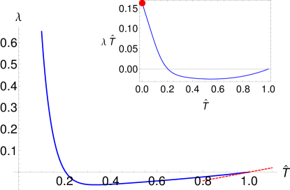
Their stability is controlled by λ1subscript𝜆1\lambda_{1}. In fig. 6 we plot the eigenvalue λ1subscript𝜆1\lambda_{1} as a function of the scaled temperature T^=T/c^𝑇𝑇𝑐\hat{T}=T/c for a fixed value ϕ^=αc^italic-ϕ𝛼𝑐\hat{\phi}=\alpha c, as well as the theoretical predictions near Tcsubscript𝑇𝑐T_{c} (91) and T0similar-to-or-equals𝑇0T\simeq 0 (93).

Refer to caption
Figure 6: Eigenvalue λ1subscript𝜆1\lambda_{1} as a function of the temperature T^^𝑇\hat{T}, for a fixed α^=0.2^𝛼0.2\hat{\alpha}=0.2. The red dashed line gives the theoretical prediction near the critical temperature (eq.(91)). The figure in the inset is in agreement with (eq.(93)), which holds for T0𝑇0T\to 0 and gives λ^=λ/ϕcI0(ϕc)1^𝜆𝜆superscriptitalic-ϕ𝑐subscript𝐼0italic-ϕ𝑐1\hat{\lambda}=\lambda/\rme^{-\phi c}I_{0}(\phi c)\to 1.

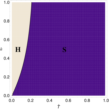
In fig. 7 we show the critical line in the parameter space T^,α^^𝑇^𝛼\hat{T},\hat{\alpha} separating the region (S), where symmetric mixtures are stable, from the region (H) where they are unstable. The phase diagram shows that for huge regions of the tunable parameters (noise and storage load) the system is able to recall all the stored patterns in parallel and symmetrically. However, for low temperature, symmetry of patterns is broken and should not be assumed in analysis at zero temperature [7]. We propose in the next subsection the hierarchical structure of the steady state at zero temperature.
Refer to caption
Figure 7: Phase diagram in the regime δ=γ𝛿𝛾\delta=\gamma. In the parameter space (T^,α^)^𝑇^𝛼(\hat{T},\hat{\alpha}) the purple area represents the region where symmetric mixtures exist and are stable, which correspond to λ1<0subscript𝜆10\lambda_{1}<0. The area denoted by H𝐻H represents the region where we expect a hierarchical retrieval.

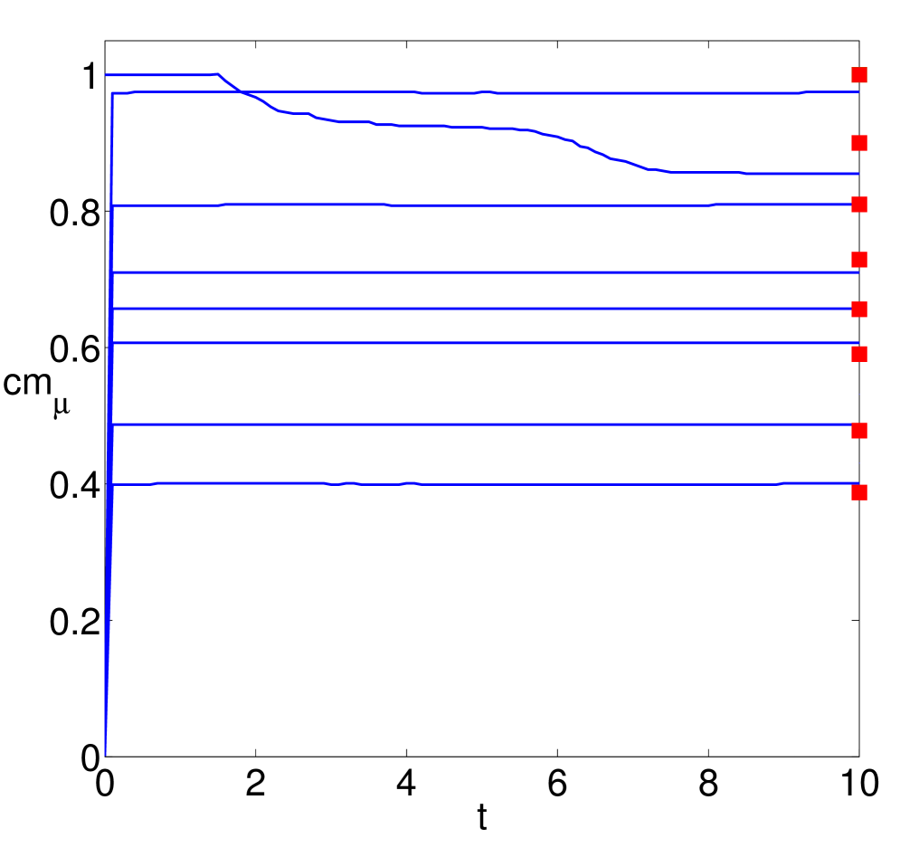
In fig. 8 (left panel) we show Monte-Carlo simulations of a system with N=104𝑁superscript104N=10^{4} spins, evolving according to sequential Glauber dynamics with δ=γ=0.25𝛿𝛾0.25\delta=\gamma=0.25, T=0.75𝑇0.75T=0.75, c=0.8𝑐0.8c=0.8 and α=1𝛼1\alpha=1. Such a choice of the parameters corresponds to the region in the phase space where symmetric mixtures are stable. Overlaps with different patterns are seen to evolve to symmetric, non-zero values in agreement, up to finite-size effects, with the values predicted by the theory (95).

In conclusion, pattern cross-talk manifests in this regime as a noise with the random-walk distribution (86), which has the effect of shrinking the amplitude of symmetric mixtures with respect to the regime without cross-talk, where Pϕ(z)subscript𝑃italic-ϕ𝑧P_{\phi}(z) crosses over to a delta function centered in z=0𝑧0z=0 and amplitudes are given by the Curie-Weiss equation (46).

5.1.1 Extending the hierarchical ansatz to the medium storage regime

As explained above, symmetric mixtures are unstable at low temperature. It is not a priori clear how the symmetry is broken, however for T0𝑇0T\to 0 one may expect that the systems retrieves patterns in a hierarchical fashion similar to the one found in the low storage regime. Reasoning as in [1, 10, 6], we can assume that the system starts aligning its entries to the non-zero entries of the first pattern, which are cN1γ𝑐superscript𝑁1𝛾cN^{1-\gamma}, sparing NcN1γ𝑁𝑐superscript𝑁1𝛾N-cN^{1-\gamma} entries of 𝝈𝝈\sigma to align with the cN1γ𝑐superscript𝑁1𝛾cN^{1-\gamma} non-zero entries of the second pattern and so on. Proceeding iteratively, we get to a heuristic general expression

mμ=(1cNγ)μ1μ=1,,ϕNγ,formulae-sequencesubscript𝑚𝜇superscript1𝑐superscript𝑁𝛾𝜇1𝜇1italic-ϕsuperscript𝑁𝛾\displaystyle m_{\mu}=\bigg{(}1-\frac{c}{N^{\gamma}}\bigg{)}^{\mu-1}\quad\quad\mu=1,\ldots,\phi N^{\gamma}, (96)
Refer to caption
Refer to caption
Figure 8: Monte-Carlo simulations of a system with N=104𝑁superscript104N=10^{4} spins, γ=δ=0.25𝛾𝛿0.25\gamma=\delta=0.25 and α=1𝛼1\alpha=1 evolving according to sequential Glauber dynamics. We plot the overlaps mμsubscript𝑚𝜇m_{\mu} with different patterns 𝝃μsuperscript𝝃𝜇{\mbox{\boldmath$\xi$}}^{\mu} as a function of time t𝑡t. Left: T^=0.75^𝑇0.75\hat{T}=0.75, c=0.8𝑐0.8c=0.8. Red markers represent the values theoretically predicted by (95). Right: T^=0.01^𝑇0.01\hat{T}=0.01, c=1𝑐1c=1. Red markers represent the values heuristically predicted by the ansatz (96) at T=0𝑇0T=0.

whose stability at T=0𝑇0T=0 is given by the eigenvalues

λμsubscript𝜆𝜇\displaystyle\lambda_{\mu} =\displaystyle= β^P(mμ)μ=1,,ϕNγformulae-sequence^𝛽𝑃subscript𝑚𝜇𝜇1italic-ϕsuperscript𝑁𝛾\displaystyle\hat{\beta}P(m_{\mu})\quad\quad\mu=1,\ldots,\phi N^{\gamma}
λνsubscript𝜆𝜈\displaystyle\lambda_{\nu} =\displaystyle= β^P(0)ν=ϕNγ+1,,αNγformulae-sequence^𝛽𝑃0𝜈italic-ϕsuperscript𝑁𝛾1𝛼superscript𝑁𝛾\displaystyle\hat{\beta}P(0)\quad\quad\nu=\phi N^{\gamma}+1,\ldots,\alpha N^{\gamma} (97)

where P𝑃P is given in (44). As in Sec. (4.2), the probability P(0)𝑃0P(0) is bounded by the probability of drawing 𝝃=0𝝃0{\mbox{\boldmath$\xi$}}=0, Pϕ(0)(1cNγ)ϕNγcϕ>0subscript𝑃italic-ϕ0superscript1𝑐superscript𝑁𝛾italic-ϕsuperscript𝑁𝛾similar-to-or-equalssuperscript𝑐italic-ϕ0P_{\phi}(0)\geq(1-cN^{-\gamma})^{\phi N^{\gamma}}\simeq\rme^{-c\phi}>0, hence a necessary condition to have stability is α=ϕ𝛼italic-ϕ\alpha=\phi. Monte-Carlo simulations at small temperature support the validity of the ansatz (96) for γ>0𝛾0\gamma>0, with ϕ=αitalic-ϕ𝛼\phi=\alpha (see fig. 8, right panel). Remarkably, the first pattern of the hierarchy is recalled without errors, besides the presence of cross-talk.

5.2 Strong interference for δ>γ𝛿𝛾\delta>\gamma

In Sec 5.1 we have shown that solutions in the form 𝐦=m(1,,1,0,,0)𝐦𝑚1100{\bf m}=m(1,\ldots,1,0,\ldots,0) were always unstable unless ϕNγ=Pitalic-ϕsuperscript𝑁𝛾𝑃\phi N^{\gamma}=P. Hence, for δ>γ𝛿𝛾\delta>\gamma we assume that the number of condensed patterns is n=ψNδ𝑛𝜓superscript𝑁𝛿n=\psi N^{\delta}. The amplitude of symmetric mixtures follows from (95) as

m=z=αNδαNδPψ(z)tanh[β^m(1+z)]𝑚superscriptsubscript𝑧𝛼superscript𝑁𝛿𝛼superscript𝑁𝛿subscript𝑃𝜓𝑧^𝛽𝑚1𝑧\displaystyle m=\sum_{z=-\alpha N^{\delta}}^{\alpha N^{\delta}}P_{\psi}(z)\tanh[\hat{\beta}m(1+z)] (98)

where

Pψ(z)=ππω2πωz+cψNδγ(cosω1).subscript𝑃𝜓𝑧superscriptsubscript𝜋𝜋differential-d𝜔2𝜋superscript𝜔𝑧𝑐𝜓superscript𝑁𝛿𝛾𝜔1\displaystyle P_{\psi}(z)=\int_{-\pi}^{\pi}\frac{\rmd\omega}{2\pi}\rme^{-\rmi\omega z+c\psi N^{\delta-\gamma}(\cos\omega-1)}. (99)

For large N𝑁N, the integral above has most of its mass concentrated around ω=0𝜔0\omega=0, hence we can use the small-ω𝜔\omega expansion in the exponent

Pψ(z)subscript𝑃𝜓𝑧\displaystyle P_{\psi}(z) =\displaystyle= ππω2πωzcψNδγ2ω2=z2/2cψNδγ2πcψNδγsuperscriptsubscript𝜋𝜋differential-d𝜔2𝜋superscript𝜔𝑧𝑐𝜓superscript𝑁𝛿𝛾2superscript𝜔2superscriptsuperscript𝑧22𝑐𝜓superscript𝑁𝛿𝛾2𝜋𝑐𝜓superscript𝑁𝛿𝛾\displaystyle\int_{-\pi}^{\pi}\frac{\rmd\omega}{2\pi}\rme^{-\rmi\omega z-\frac{c\psi N^{\delta-\gamma}}{2}\omega^{2}}=\frac{\rme^{-z^{2}/2c\psi N^{\delta-\gamma}}}{\sqrt{2\pi c\psi N^{\delta-\gamma}}} (100)

where in the second equality we rescaled ωω/cψNδγ𝜔𝜔𝑐𝜓superscript𝑁𝛿𝛾\omega\to\omega/\sqrt{c\psi N^{\delta-\gamma}} and extended the rescaled boundaries to infinity, due to the fast decay of the exponential at large values of ω𝜔\omega, and performed the Gaussian integral. Hence, the cross-talk between the large number of insufficiently diluted condensed patterns manifests as a Gaussian noise, in this regime, as expected from the asymptotics of the random-walk distribution for large times. The variance of the Gaussian noise is given by ϕ^=cϕ^italic-ϕ𝑐italic-ϕ\hat{\phi}=c\phi where ϕ=ψNδγitalic-ϕ𝜓superscript𝑁𝛿𝛾\phi=\psi N^{\delta-\gamma} quantifies the level of interference between patterns. The effect of interference on the symmetric mixtures is stronger in this regime, leading to smaller amplitudes of the symmetric recall. We anticipate, however, that in the limit of large interference, cϕ1much-greater-than𝑐italic-ϕ1c\phi\gg 1, symmetric mixtures are unstable and a parallel recall is still accomplished by the system, in contrast with predictions in [7], where symmetric mixtures were assumed.

Linear stability analysis of the symmetric mixtures 𝐦=m(1,,1,0,0)𝐦𝑚1100{\bf m}=m(1,\ldots,1,0\ldots,0) with n=ψNδ𝑛𝜓superscript𝑁𝛿n=\psi N^{\delta} can be performed as in Sec 5.1, by identifying ϕ=ψNδγitalic-ϕ𝜓superscript𝑁𝛿𝛾\phi=\psi N^{\delta-\gamma}. For TTcsimilar-to-or-equals𝑇subscript𝑇𝑐T\simeq T_{c}, we get from equations (89) and (90),

q1ϵ(1+23cψNδγ),qϵ(113cψNδγ)formulae-sequencesimilar-to-or-equalssubscript𝑞1italic-ϵ123𝑐𝜓superscript𝑁𝛿𝛾similar-to-or-equals𝑞italic-ϵ113𝑐𝜓superscript𝑁𝛿𝛾\displaystyle q_{1}\simeq\epsilon\Big{(}1+\frac{2}{3c\psi N^{\delta-\gamma}}\Big{)},\quad\quad\quad q\simeq\epsilon\Big{(}1-\frac{1}{3c\psi N^{\delta-\gamma}}\Big{)} (101)

which give

λ1ϵ1cψNδγ,λ2ϵ13cψNδγ.formulae-sequencesimilar-to-or-equalssubscript𝜆1italic-ϵ1𝑐𝜓superscript𝑁𝛿𝛾similar-to-or-equalssubscript𝜆2italic-ϵ13𝑐𝜓superscript𝑁𝛿𝛾\displaystyle\lambda_{1}\simeq-\epsilon\frac{1}{c\psi N^{\delta-\gamma}},\quad\quad\quad\lambda_{2}\simeq\epsilon\frac{1}{3c\psi N^{\delta-\gamma}}. (102)

For any large but finite N𝑁N, symmetric mixtures are stable only if all components are recalled, as λ1<0subscript𝜆10\lambda_{1}<0 and λ2>0subscript𝜆20\lambda_{2}>0. In the thermodynamic limit, (102) vanish, and stability cannot be assessed to linear order in ϵitalic-ϵ\epsilon. In the low temperature limit, T0𝑇0T\to 0, we have, similarly to (93), (94),

q11Pψ(1),λ1β^Pψ(1)formulae-sequencesubscript𝑞11subscript𝑃𝜓1subscript𝜆1^𝛽subscript𝑃𝜓1\displaystyle q_{1}\to 1-P_{\psi}(-1),\hskip 56.9055pt\lambda_{1}\to\hat{\beta}P_{\psi}(1) (103)
q1Pψ(0),λ2β^Pψ(0).formulae-sequence𝑞1subscript𝑃𝜓0subscript𝜆2^𝛽subscript𝑃𝜓0\displaystyle q\to 1-P_{\psi}(0),\hskip 65.44142pt\lambda_{2}\to\hat{\beta}P_{\psi}(0). (104)

For large N𝑁N, Pψ(1)Pψ(0)N(γδ)/2/2πcψsimilar-to-or-equalssubscript𝑃𝜓1subscript𝑃𝜓0similar-to-or-equalssuperscript𝑁𝛾𝛿22𝜋𝑐𝜓P_{\psi}(1)\simeq P_{\psi}(0)\simeq N^{(\gamma-\delta)/2}/\sqrt{2\pi c\psi} and we get

λ1λ2β^N(γδ)/22πcψsimilar-to-or-equalssubscript𝜆1subscript𝜆2^𝛽superscript𝑁𝛾𝛿22𝜋𝑐𝜓\lambda_{1}\simeq\lambda_{2}\to\frac{\hat{\beta}N^{(\gamma-\delta)/2}}{\sqrt{2\pi c\psi}} (105)

hence for any large and finite N𝑁N, both eigenvalues are positive and symmetric mixtures are unstable, indicating that a hierarchical retrieval must take place. We can compute λ1,2subscript𝜆12\lambda_{1,2} numerically from (89, 90) by using (87,88) where Pϕsubscript𝑃italic-ϕP_{\phi} is replaced with (100) and the amplitude m𝑚m is determined from (98). In Fig. 9 we plot the eigenvalue λ1subscript𝜆1\lambda_{1} as a function of T^^𝑇\hat{T} at a large fixed value of ϕ^^italic-ϕ\hat{\phi}, as well as the predicted limits for T^0^𝑇0\hat{T}\to 0 and T^1^𝑇1\hat{T}\to 1 given in (102) and (105) respectively. We check numerically that λ2subscript𝜆2\lambda_{2} stays positive for any temperature below criticality.
Refer to caption
Figure 9: Eigenvalue λ1subscript𝜆1\lambda_{1} as a function of the temperature T^^𝑇\hat{T}, for a fixed ϕ^=cϕ=5^italic-ϕ𝑐italic-ϕ5\hat{\phi}=c\phi=5. The red dashed line gives the theoretical prediction near the critical temperature (102). The figure in the inset shows agreement with (105), which gives λ1/(T^)N(γδ)/22πcψsubscript𝜆1^𝑇superscript𝑁𝛾𝛿22𝜋𝑐𝜓\lambda_{1}/(\hat{T})\to\frac{N^{(\gamma-\delta)/2}}{\sqrt{2\pi c\psi}} as T^0^𝑇0\hat{T}\to 0 (red marker).

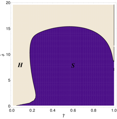
A contour plot of the critical line where λ1=0subscript𝜆10\lambda_{1}=0 in the Tc𝑇𝑐T-c place is shown in Fig. 10. Again, we identify the region S where symmetric mixtures are stable and an H region where these become unstable. We note that for strong interference or low temperature the symmetry of pattern is broken.
Refer to caption
Figure 10: Phase diagram in the parameter space (T,c)𝑇𝑐(T,c) for the case δ>γ𝛿𝛾\delta>\gamma. The (S) area represents the region where the symmetric mixtures are stable, while the (H) region is characterised by hierarchical states. The (S) region is obtained as the contour plot of the equation λ1=0subscript𝜆10\lambda_{1}=0 solved numerically together with equation (98).
Refer to caption
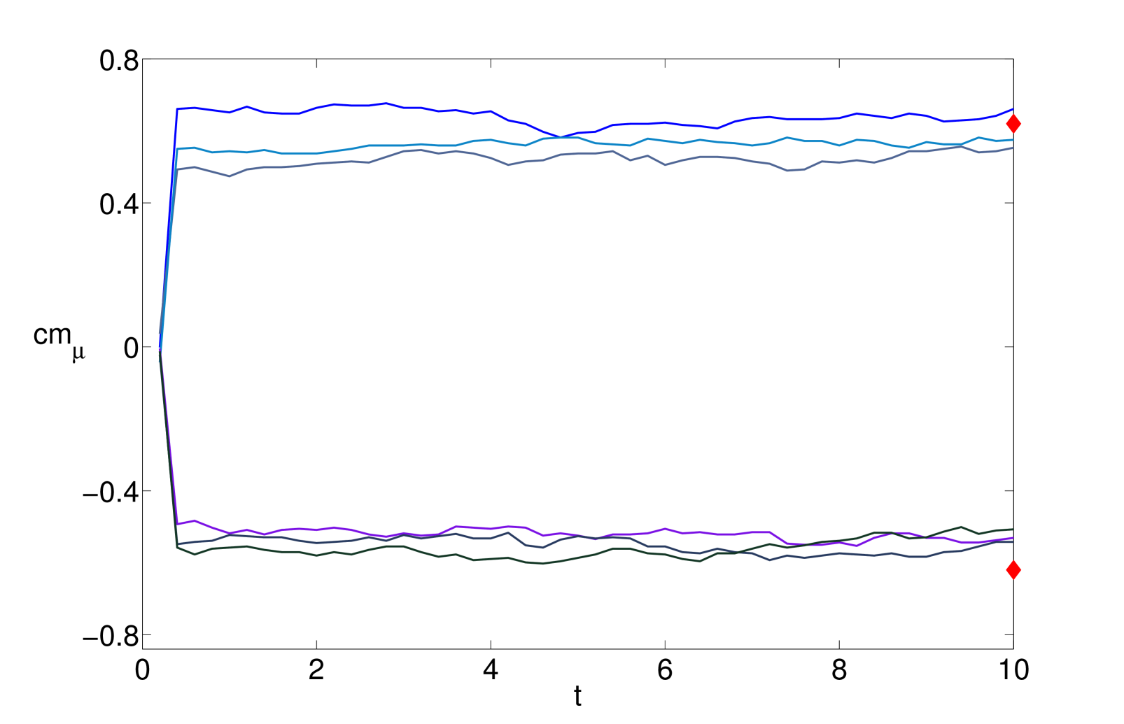
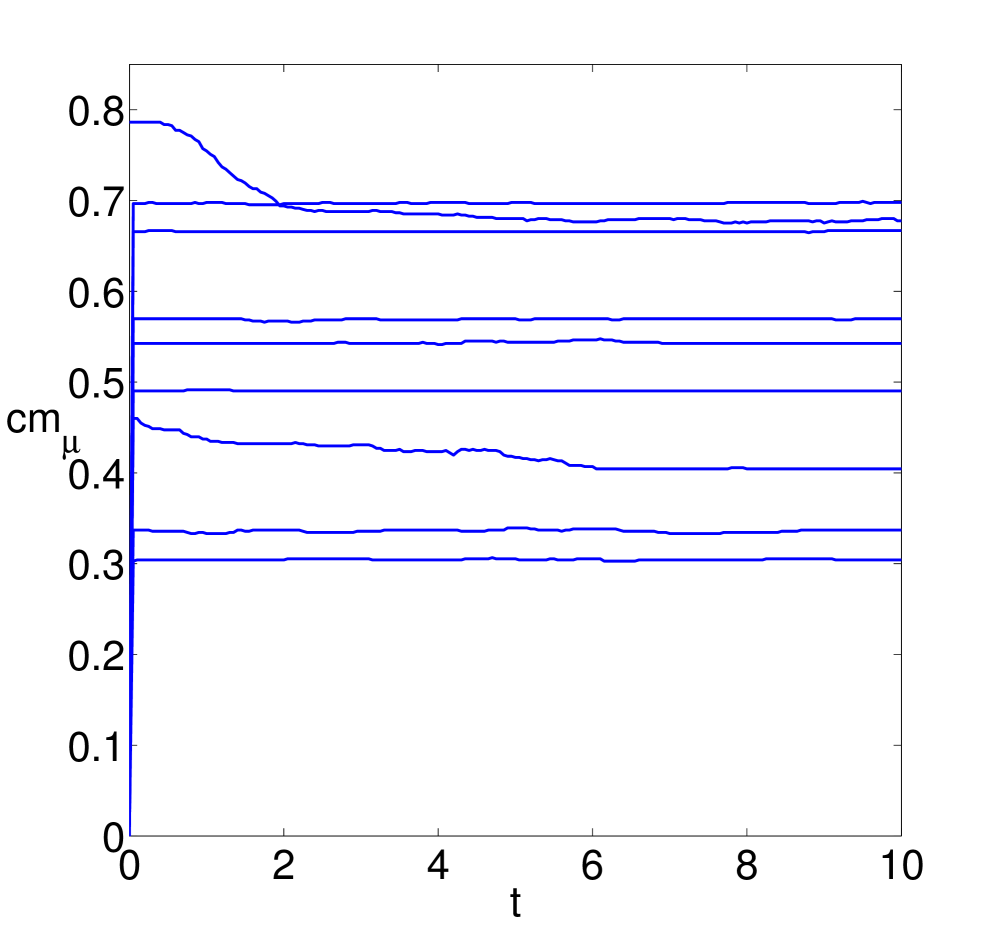
Figure 11: Monte Carlo simulations with N=104𝑁superscript104N=10^{4} spins. We plot the overlaps mμsubscript𝑚𝜇m_{\mu} with different patterns ξμsubscript𝜉𝜇\xi_{\mu}, as a function of time t𝑡t, for T^=0.015^𝑇0.015\hat{T}=0.015, c=0.8𝑐0.8c=0.8, δ=0.25𝛿0.25\delta=0.25, γ=0.2𝛾0.2\gamma=0.2 and α=1𝛼1\alpha=1.

However, in this regime, it is more difficult to predict how the symmetry of patterns is broken, even at low temperature, due to the presence of a strong interference between patterns. In particular, it is not a priori clear whether a hierarchical retrieval involves all patterns or just a fraction of them. At zero temperature one may expect that a number of patterns will show an overlap 𝒪(1)𝒪1{\mathcal{O}}{(1)} with the system configuration. Assuming that the number of these patterns is 𝒪(Nγ)𝒪superscript𝑁𝛾{\mathcal{O}}{(N^{\gamma})} and the remaining (uncondensed) 𝒪(Nδ)𝒪superscript𝑁𝛿{\mathcal{O}}{(N^{\delta})} patterns have an overlap with the system configuration 𝒪(Nγ12)𝒪superscript𝑁𝛾12\mathcal{O}(N^{\frac{\gamma-1}{2}}), we can write the noise distribution by splitting the contribution from the condensed (labelled by μ𝜇\mu) and the uncondensed (labelled by ρ𝜌\rho) patterns

P(z|𝐦)=π+πz^2πzz^+cNγμψNγ(cos(z^mμ)1)c2NγραNδmρ2z^2𝑃conditional𝑧𝐦superscriptsubscript𝜋𝜋differential-d^𝑧2𝜋superscript𝑧^𝑧𝑐superscript𝑁𝛾superscriptsubscript𝜇𝜓superscript𝑁𝛾^𝑧subscript𝑚𝜇1superscript𝑐2superscript𝑁𝛾superscriptsubscript𝜌𝛼superscript𝑁𝛿superscriptsubscript𝑚𝜌2superscript^𝑧2\displaystyle P(z|{\bf m})=\int_{-\pi}^{+\pi}\frac{\rmd\hat{z}}{2\pi}\rme^{\rmi z\hat{z}+\frac{c}{N^{\gamma}}\sum_{\mu}^{\psi N^{\gamma}}(\cos(\hat{z}m_{\mu})-1)}\rme^{-\frac{c}{2N^{\gamma}}\sum_{\rho}^{\alpha N^{\delta}}m_{\rho}^{2}\hat{z}^{2}} (106)

where we have Taylor expanded the mρsubscript𝑚𝜌m_{\rho}-dependent terms for mρsubscript𝑚𝜌m_{\rho} small. When N𝑁N is large,

P(z|𝐦)P(z|{mμ})+𝒪(Nδ1)similar-to-or-equals𝑃conditional𝑧𝐦𝑃conditional𝑧subscript𝑚𝜇𝒪superscript𝑁𝛿1\displaystyle P(z|{\bf m})\simeq P(z|\{m_{\mu}\})+\mathcal{O}(N^{\delta-1}) (107)

and the evolution of the uncondensed patterns is given, to leading orders, by

mρtzP(z|{mμ})tanh[β^(mρ+z)]mρ+𝒪(Nδ1)similar-to-or-equalsdifferential-dsubscript𝑚𝜌differential-d𝑡differential-d𝑧𝑃conditional𝑧subscript𝑚𝜇^𝛽subscript𝑚𝜌𝑧subscript𝑚𝜌𝒪superscript𝑁𝛿1\displaystyle\frac{\rmd m_{\rho}}{\rmd t}\simeq\int\rmd zP(z|\{m_{\mu}\})\tanh[\hat{\beta}(m_{\rho}+z)]-m_{\rho}+\mathcal{O}(N^{\delta-1}) (108)

which depends on the noise distribution of condensed patterns {mμ}subscript𝑚𝜇\{m_{\mu}\} only. Taylor expanding for small mρsubscript𝑚𝜌m_{\rho} we obtain

mρtmρ[β^zP(z|{mμ})(1tanh2(β^z))1]+𝒪(Nδ1)similar-to-or-equalsdifferential-dsubscript𝑚𝜌differential-d𝑡subscript𝑚𝜌delimited-[]^𝛽differential-d𝑧𝑃conditional𝑧subscript𝑚𝜇1superscript2^𝛽𝑧1𝒪superscript𝑁𝛿1\displaystyle\frac{\rmd m_{\rho}}{\rmd t}\simeq m_{\rho}\bigg{[}\hat{\beta}\int\rmd zP(z|\{m_{\mu}\})(1-\tanh^{2}(\hat{\beta}z))-1\bigg{]}+\mathcal{O}(N^{\delta-1}) (109)

and for T0𝑇0T\to 0 we get

dmρdtmρ[β^P(0|{mμ})1].similar-to-or-equals𝑑subscript𝑚𝜌𝑑𝑡subscript𝑚𝜌delimited-[]^𝛽𝑃conditional0subscript𝑚𝜇1\displaystyle\frac{dm_{\rho}}{dt}\simeq m_{\rho}[\hat{\beta}P(0|\{m_{\mu}\})-1]. (110)

As explained in 5.1.1, P(0|{mμ})eϕc𝑃conditional0subscript𝑚𝜇superscript𝑒italic-ϕ𝑐P(0|\{m_{\mu}\})\geq e^{-\phi c} This suggests that the system will attempt to recall hierarchically all patterns, as supported by Monte-Carlo simulations shown in fig. 11. However, the retrieval degrades with respect to the one described in (96), valid at the onset of pattern cross-talk, where the first pattern in the hierarchy was retrieved without errors.

6 Conclusions

In this work we analysed the dynamics of associative memories with diluted patterns, in different regimes of pattern dilution and storage load (away from saturation). We derived equations for the dynamics of a set of macroscopic order parameters, quantifying the simultaneous pattern retrieval of the system, from the microscopic evolution of the network dynamics. Results show that the network is able to accomplish a parallel retrieval of all the stored patterns, in the whole phase diagram, although the nature of the retrieval varies in different regions of the phase diagram. We analysed the structure and stability of the steady states solutions to the dynamical equations for the order parameters, for different ranges of the tunable parameters T,γ,δ𝑇𝛾𝛿T,\gamma,\delta, controlling noise, dilution and storage load, respectively.
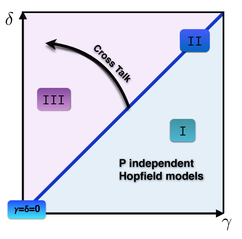
Refer to caption
Figure 12: Schematic phase space (γ,δ)𝛾𝛿(\gamma,\delta). In region I (δ<γ)𝛿𝛾(\delta<\gamma), we have a set of P𝑃P independent ferromagnets and parallel retrieval is accomplished in a symmetrical fashion. In region II cross-talk between patterns appears; the intensity of symmetric recall is decreased due to the presence of a noise, whose distribution is identical to the one of a lazy, unbiased random walker, and the region of stability of the symmetric retrieval is provided in the phase diagram (fig. 7). A similar behaviour is found for δ=γ=0𝛿𝛾0\delta=\gamma=0, but the region of stability of the symmetric region shrinks (fig. 3), due to the noise distribution retaining a pattern dependence (Sec. 3.2). Finally, in region III, cross-talk effects are strong and increase the larger δ𝛿\delta and the smaller γ𝛾\gamma. These decrease the strength of symmetric retrieval via a Gaussian interference noise, and are seen to degrade gradually the hierarchical retrieval of the network, which thus retains its parallel processing capabilities.

We identified three regimes (see fig. 12): (I) δ<γ𝛿𝛾\delta<\gamma, (II) δ=γ𝛿𝛾\delta=\gamma and (III) δ>γ𝛿𝛾\delta>\gamma. In (I) there is no interference between patterns as these are relatively low in number and sufficiently diluted, so the network behaves as a set of P𝑃P independent ferromagnets each evolving according to the Curie-Weiss equation. As a result, the parallel retrieval accomplished by the system in this regime is symmetric for any temperature below criticality. In (II) a pattern cross-talk appears and symmetric mixtures are no longer stable for all temperatures below criticality. We derived the phase diagram showing their region of stability in the parameter space. The cross-talk between patterns manifests on symmetric mixtures as a noise with the distribution of a lazy random walker, taking discrete steps at discrete time (for γ=0𝛾0\gamma=0) and in continuous time (for γ>0𝛾0\gamma>0). The laziness of the random walker is due to pattern dilution and removes the periodicity in the return times, which is responsible for the different role played by even and odd mixtures, in the traditional (i.e. undiluted) Hopfield model, at zero temperature. The region where symmetric mixtures are stable is broad for γ>0𝛾0\gamma>0, where the noise distribution is pattern-independent, whereas the retrieval is mostly hierarchic for γ=0𝛾0\gamma=0, where the symmetry of patterns is mostly a close-to-criticality effect. We rectify the result of previous analysis at zero temperature, which assumed symmetry of patterns, and provide a heuristic expression for the shape of the steady state solution at zero temperature, which finds very good agreement with numerical simulations. Finally, in (III), the effect of cross-talk manifests on symmetric mixtures as a Gaussian noise, whose variance is directly related to the level of pattern interference, which decreases the quality of parallel retrieval. We derive the region of stability of symmetric mixtures and show that for large interference or low temperature, symmetric mixtures are unstable. In particular, at zero temperature the system is able to retrieve all patterns in a hierarchical fashion, despite the presence of strong interference may suggest that no retrieval is accomplished in this regime [7].

Acknowledgements

We thank Prof. A. C. C. Coolen for useful discussions and helpful advice.

References

References

  • [1] Agliari E, Barra A, Galluzzi A, Guerra F, Moauro F 2012 Phys. Rev. Lett. 109, Issue 26.
  • [2] Hopfield J J 1982 Proc. Natl Acad. Sci. USA 79 2554-2558.
  • [3] Amit D J, Gutfreund H and Sompolinsky H 1895 Phys. Rev. A 32, 1007–1018 .
  • [4] Amit D J, Gutfreund H, Sompolinsky H 1985 Phys. Rev. Lett. 55, 1530-1533.
  • [5] Coolen ACC, Kuehn R and Sollich P 2005 Theory of neural information processing systems, ( Oxford University Press, Oxford).
  • [6] Agliari E, Barra A, Bartolucci S, Galluzzi A, Guerra F and Moauro F 2013 Phys. Rev. E 87, 042701.
  • [7] Agliari E, Annibale A, Barra A, Coolen A C C and Tantari D 2013 J. Phys. A 46 Issue 33.
  • [8] Agliari E, Annibale A, Barra A, Coolen A C C and Tantari D 2013 J. Phys. A 46 Issue 41.
  • [9] Sollich P, Tantari D, Annibale A and Barra A 2014 Preprint arXiv1404.3654.
  • [10] Agliari E, Barra A, Galluzzi A and Isopi M 2012 arXiv 1304.4488.
  • [11] Coolen A C C and Ruijgrok W Th 1988 Phys. Rev. A 38, 4253–4255 .
  • [12] Sherrington D, Coolen A C C and Laughton S N 1996 CNLS Newsletter(Los Alamos) 124 1-12.
  • [13] Van Kampen N G, 1992 Stochastic Processes in Physics and Chemistry, (North-Holland, Amsterdam).
  • [14] Abramowitz M, Stegun I A 1972 Handbook of Mathematical Functions, (Dover, New York).
  • [15] Amit D J 1989 Modelling brain function, (Cambridge University Press).
  • [16] Mezard M, Parisi G and Virasoro A 1987 Spin glass theory and beyond, (World Scientific, Singapore).