Oscillations in Spurious States of the Associative Memory Model with Synaptic Depression
Abstract
The associative memory model is a typical neural network model, which can store discretely distributed fixed-point attractors as memory patterns. When the network stores the memory patterns extensively, however, the model has other attractors besides the memory patterns. These attractors are called spurious memories. Both spurious states and memory states are equilibrium, so there is little difference between their dynamics. Recent physiological experiments have shown that short-term dynamic synapse called synaptic depression decreases its transmission efficacy to postsynaptic neurons according to the activities of presynaptic neurons. Previous studies have shown that synaptic depression induces oscillation in the network and decreases the storage capacity at finite temperature. How synaptic depression affects spurious states, however, is still unclear. We investigate the effect of synaptic depression on spurious states through Monte Carlo simulation. The results demonstrate that synaptic depression does not affect the memory states but mainly destabilizes the spurious states and induces the periodic oscillations.
1 Introduction
The associative memory model is a typical neural network model. The network in this model has discretely distributed fixed-point attractors, and it can store these point attractors as memory patterns by using Hebbian rule[1, 2, 3]. Given an initial state near a memory pattern, the network generally converges on the memory pattern. The associative memory model has other attractors, however, besides the stored memory patterns in extensive loading cases, which means that the number of memory patterns is on the order of the number of neurons. These other attractors are called spurious memories. A state in which the network converges on a memory pattern is called a memory state, while a state in which the network converges on a spurious memory is called a spurious state. There is little difference in network dynamics between memory states and spurious states, because both states are equilibrium. This is a serious problem in applying the associative memory model as an information processing model.
Recent physiological experiments have shown that the efficacy of synaptic transmission changes in a short period of time. For example, dynamic synapses can decrease their transmission efficacy to postsynaptic neurons according to the activities of presynaptic neurons[4, 5, 6, 7]. This phenomenon is called synaptic depression and is a kind of short-term synaptic plasticity. Previous studies have revealed that synaptic depression destabilizes attractors and induces switching phenomena among them when the number of memory patterns is much smaller than the number of neurons, i.e., in finite loading cases[8, 9]. However, the network has many attractors including spurious memories in extensive loading cases. Effects of synaptic depression on these attractors have not been investigated in detail. Synaptic depression may induce difference between memory states and spurious states.
In this study, we apply Monte Carlo simulation in order to reveal effects of synaptic depression on attractors including spurious memories. As a result, we find that synaptic depression does not affect memory states but mainly destabilizes spurious states and induces periodic oscillations. This result suggests that incorporating synaptic depression would improve the performance of the associative memory model as an information processing model.
This paper consists of four sections, including this Introduction. In Sect. 2 we describe the associative memory model with synaptic depression. Section 3 describes and analyzes the simulation results. Finally, in Sect. 4 we summarize the results.
2 Model
In this section, we introduce an associative memory model with synaptic depression, consisting of fully connected McCulloch-Pitts neurons. If the -th neuron fires at time , its state is represented by ; otherwise, . The network state at time is denoted by a variable . Each neuron is updated with the following probability:
| (1) |
| (2) |
Here, represents an internal potential in the -th neuron at time , and is a function taking continuous values on . We consider an inverse temperature and then we define the function as
| (3) |
The strength of a synaptic connection between the -th and -th neurons is denoted by and given by the following:
| (4) | |||||
| (5) |
where is the efficacy of synaptic transmission and takes continuous values in the range [7, 8]. Here, represents the fraction of released neurotransmitter in the absence of depression, and is a time constant for the recovery process. The absolute strength of synaptic connection, , is given by the following Hebbian rule:
| (6) |
Here, corresponds to the number of memory patterns stored in the network. The ratio of the number of neurons, , to the number of memory patterns, , is called the loading ratio , i.e., . The stored memory pattern is stochastically provided by the following:
| (7) |
3 Results
In this section, we show the results obtained from Monte Carlo simulation with the model defined in Sect. 2. In order to describe macroscopic state of a network, we define an overlap between the -th memory pattern and the network state as
| (8) |
The overlap corresponds to the direction cosine between the -th memory pattern and the state of the network. When the state completely matches the memory pattern , the overlap takes the value . On the other hand, when is orthogonal to , then takes the value . The initial network state is given by the following probability:
| (9) |
The expectation of the overlap provided in this way becomes in the limit of . Therefore, corresponds to the initial overlap.
| (a) | 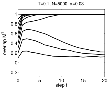 |
(b) | 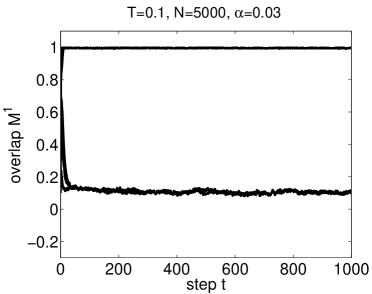 |
| (c) | 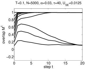 |
(d) | 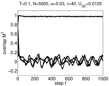 |
3.1 Dependence of overlap on step
In this subsection, we show how synaptic depression affects the dependence of the overlap on step . Figure 1 shows the dependence obtained from Monte Carlo simulation with , , and loading ratio , i.e., . Initial states are provided with initial overlap by varying the value from to at intervals of .
Figure 1(a) shows the case without synaptic depression from to , while Fig. 1(b) shows the same case over a long time span, from to . When is greater than , converges to the value at large , meaning that memory retrieval succeeds. This final state corresponds to a memory state. On the other hand, when is less than , is in equilibrium, such that overlaps do not reach the value . This equilibrium is called a spurious state. In contrast, Fig. 1(c) shows the case with synaptic depression, where and . When is greater than , the network succeeds in memory retrieval; otherwise, when is less than , the network fails in memory retrieval and falls into a spurious state. Figure 1(d) shows the case with synaptic depression over a long time span, from to . Here, the overlaps in the spurious state oscillate, whereas those in the memory state converge.
Thus, from the results shown in Fig. 1, we can see that synaptic depression does not affect memory states but destabilizes spurious states and induces oscillation.
3.2 Autocorrelation functions and period of network dynamics
In order to reveal a property of the oscillations shown in Fig. 1(d), we investigate an autocorrelation function for the overlaps . This function is a measure of the dependence of on past data and is defined as
| (10) |
Here, is the number of steps in overlap , and represents the time lag between data. The sample mean of overlap , , and the sample variance, , are given by the following:
| (11) | |||||
| (12) |
Figure 2 shows the dependence of the autocorrelation function on the lag . The dashed lines represent in a memory state, while the solid lines represent in a spurious state. Note that has the values and in the cases of a memory state and a spurious state, respectively.
| (a) | 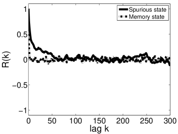 |
(b) | 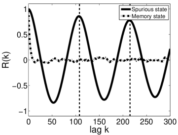 |
Figure 2(a) shows the case without synaptic depression. In both the memory state and the spurious state, rapidly decays to with increasing . This means that is not affected by past data; rather, its dynamics fluctuate randomly because of the probabilistic update given by Eq. (1).
Figure 2(b) shows the case with synaptic depression, where and . In the memory state, decays to as in the case without synaptic depression. On the other hand, in the spurious state, has high positive amplitude at and , meaning that oscillates with a period of around in terms of the time lag.
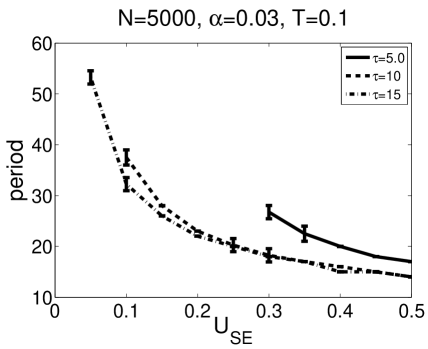
Next, we investigate how the period depends on the strength of synaptic depression. Figure 3 shows the dependence of the period on . Here, varies from to at intervals of , while is fixed at either , , or . Each line in the graph represents the mean period obtained from five simulations, and each error bar indicates three standard deviations. We find that as increases, the period decreases and then converges. We also see that when is large, it hardly affects the dependence of the period on . Finally, we find that the period decreases as the strength of the synaptic depression increases.
3.3 Effects on basin of attraction
It turns out that whether memory retrieval succeeds or not depends on the value of the initial overlap from Figs. 1(a) and 1(c). There exists a minimum value of the initial overlap , such that the network succeeds in memory retrieval, and this minimum value is called the critical overlap . The region where is called a basin of attraction, since the network converges on the memory pattern. In this subsection, we investigate the effects of synaptic depression on the basin of attraction. Figure 4 shows basins of attraction obtained from 12 simulations. Each cell represents the number of successful memory retrievals. In each trial run, varies from to at intervals of , and varies from to at intervals of . We define the condition that is greater than or equal to at as a successful memory retrieval. The boundary between the white and black regions corresponds to the critical overlap .
Figure 4(a) shows the case without synaptic depression. It turns out that the value of the critical overlap increases with . Furthermore, the value of drastically increases to at around . This value of is called the memory storage capacity[10, 11, 12]. When is larger than the memory storage capacity, the network cannot retrieve memory patterns even though it starts from a memory pattern. Figure 4(b) shows the case with synaptic depression, where and . As in the previous case, we see that the value of the critical overlap increases with , but in this case drastically increases to at around . This decrease in memory storage capacity at finite temperature as a result of synaptic depression was revealed previously[12]. Note that when is less than , the dependence of on shows little difference between the cases with and without synaptic depression, as seen by comparing Figs. 4(a) and 4(b). This means that when is less than , synaptic depression hardly affects the basin of attraction.
| (a) | 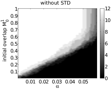 |
(b) | 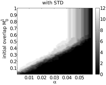 |
3.4 Trajectories of network dynamics
We find that the overlap in a spurious state oscillates periodically because of synaptic depression, as shown in Fig. 2. In order to investigate this oscillating network behavior, we next carry out principal component analysis (PCA) on the network state .
| (a) |  |
(b) | 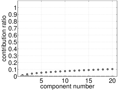 |
| (c) | 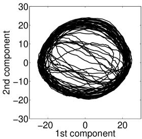 |
(d) | 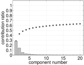 |
Figure 5 shows the results obtained from PCA. Specifically, the figure shows the trajectories expressed by the first and second principal components, and the contribution ratios, with the parameters , , , and .
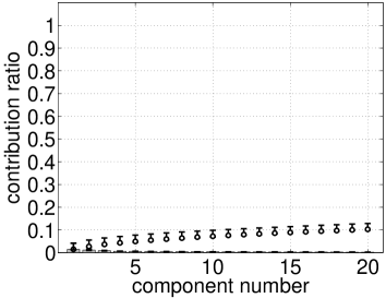
Figure 5(a) shows the case without synaptic depression. From the figure, we find that the network fluctuates randomly on the plane spanned by the first and second principal components. Figure 5(b) shows the contribution ratios and the cumulative contribution up to the 20th principal component. All the contribution ratios are lower than .
Figure 5(c) shows the case with synaptic depression, where and , the same parameters used for Fig. 1(d). The network trajectory has circular motion on the plane spanned by the first and second principal components. Figure 5(d) shows the contribution ratios and cumulative contribution up to the 20th principal component for the case with synaptic depression. The contribution ratios of both the first and second principal components are particularly high, with a sum of around
| (a) |
 (b)
(b) |
 |
| (c) |
 (d)
(d) |
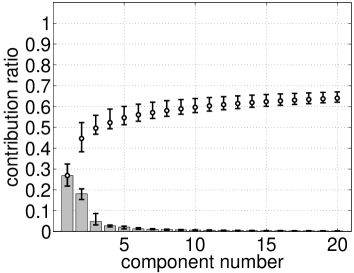 |
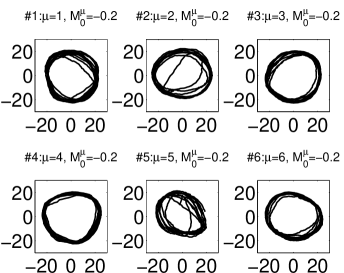
Next, we change the value of initial pattern, , and initial overlap , and then carry out 750 simulations, i.e., varying from to at intervals of , and varying from to at intervals of . We perform -step simulations, and then count out first steps as initial relaxation. Furthermore, in the case without synaptic depression, the network state in two simulations converge on memory patterns. Thus, we count out these data. We show the result of PCA on data set obtained from these simulations in Figs. 6. Figures 6(a) and 6(b) show the case without synaptic depression. Figure 6(a) shows network trajectories on a plane spanned by the first and the second principal components. We show the typical results from trials. Bars and open circles in the Fig. 6 (b) represent the median value of contribution ratio, and cumulative contribution, respectively. Error bars represent 5th-95th percentile range. We find that the networks fluctuate randomly on the high-dimensional subspace, because almost all contribution ratios are less than . Figures 6(c) and 6(d) show the case with synaptic depression, where , and . Figure 6(c) shows the network trajectories on plane consisting of the first and the second principal components. We show the typical results from trials. Bars and open circles in the Fig. 6(d) represent the median value of contribution ratio, and cumulative contribution, respectively. Error bars represent 5th-95th percentile range. We find that the network in spurious states predominantly oscillate on the plane spanned by the first and the second principal components, because contribution ratio of the first and the second principal components are higher than that of other principal component. From the result shown in Fig. 6, we can see that network in spurious states with synaptic depression oscillates circularly on low-dimensional plane, whereas network in spurious states without synaptic depression fluctuates randomly.
| (a) | 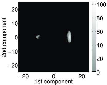 |
(b) | 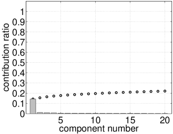 |
| (c) | 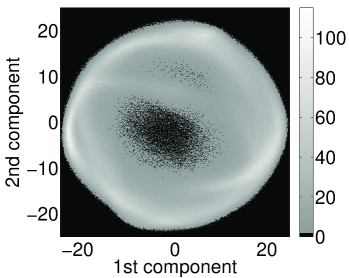 |
(d) |  |
Next, in order to investigate relationship among trajectories, we combine all network state data, , obtained from 750 different initial condition, and then carry out PCA on the data. Figures 7(a) and 7(b) show the result obtained from PCA in the case without synaptic depression. Figure 7(a) shows distribution of spurious states on plane spanned by the first and the second principal components as histogram. The distribution is shown as gray scale image, with black and white corresponding to the smallest and the largest number of spurious states, respectively. Figure 7(b) shows contribution ratio and cumulative contribution. Bar denotes contribution ratio, and open circle denotes cumulative contribution. We can see that contribution ratio of the first principal component in this combined data case is higher than separate data case. From these results, spurious states in the case without synaptic depression are separated on the plane spanned by the first and the second principal components. This result is similar to behavior of spin-glass state data of Sherrington-Kirkpatrick model obtained from PCA analysis[13]. Figures 7(c) and 7(d) show the result obtained from PCA in the case with synaptic depression, where , and . Figure 7(c) shows distribution of spurious states on plane spanned by the first and the second principal components as histogram. The distribution is shown as gray scale image, with black and white corresponding to the smallest and the largest number of spurious states, respectively. Figure 7(d) shows contribution ratio and cumulative contribution. Bar denotes contribution ratio, and open circle denotes cumulative contribution. Contribution ratio up to the third principal component is higher than other principal components. We see that network in spurious states oscillates in low-dimensional subspace, i.e. around three dimension, in the case with synaptic depression.
3.5 Eigenvectors of synaptic weight matrix
From the above, we see that network in spurious states fluctuates in high-dimensional subspace in the case without synaptic depression, whereas network oscillates in low-dimensional subspace in the case with synaptic depression. In the former case, dynamics of memory recalling in the associative memory model was discussed qualitatively by using eigenvectors of synaptic weight matrix. Kindo and Kakeya claimed that linear transformation of synaptic weight matrix is important to analyze dynamical properties[14]. Thus, in this subsection, we investigate relationship between subspace in which oscillation induced by synaptic depression occurs and subspace spanned by eigenvectors of synaptic weight matrix.
We consider synaptic weight matrix whose entry is the static weight . Eigenvector of corresponds to the -th largest eigenvalue . Here, has positive eigenvalues and zero eigenvalues. Considering component of , we see that subspace spanned by eigenvectors corresponding to positive eigenvalues is composed of memory patterns, and subspace spanned by eigenvectors corresponding to zero eigenvalues is orthogonal to subspace spanned by memory patterns.
Network state is expressed by using as
| (13) | |||||
| (14) |
Contribution ratio, , of each is defined as
| (15) |
Figure 8 shows contribution ratio, , and cumulative contribution up to , since has 150 positive eigenvalues and 4850 zero eigenvalues in this study. Bars and open circles denote contribution ratio and cumulative contribution, respectively. Figure 8(a) shows the case without synaptic depression, and Fig. 8(b) shows the case with synaptic depression, where , and . In the case without synaptic depression, we see that spurious states mainly exist in subspace which is orthogonal to memory patterns, since cumulative contribution is around at . In the case with synaptic depression, however, we see that spurious states mainly exist in subspace which is spanned by memory patterns, since cumulative contribution is around at . From the results shown in Fig. 8, we see that oscillation of network induced by synaptic depression mainly occurs on subspace spanned by memory patterns.
| (a) | 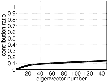 |
(b) | 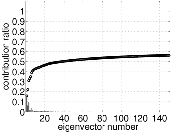 |
| (a) | 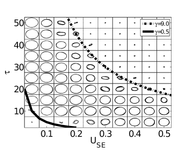 |
(b) | 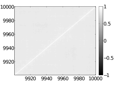 |
| (c) | 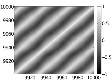 |
(d) | 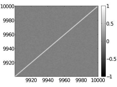 |
3.6 Phase diagram
In this subsection, we investigate how the network trajectory depends on the strength of synaptic depression. Figure 9(a) shows a phase diagram for this dependence. The horizontal axis corresponds to , and the vertical axis corresponds to . The value of varies from to at intervals of , and varies from to at intervals of . Each cell represents the network trajectory on the plane spanned by the first and second principal components. The solid and dashed lines correspond to and , respectively, where represents the strength of synaptic depression in equilibrium and is defined as [8, 12]. The trajectories have circular motion when is more than and less than or equal to .
We now consider the overlap between network states and , given by:
| (16) |
When network state at step completely matches state at step , the overlap takes the value . When network state is orthogonal to , takes the value . Lastly, takes the value when state at step is the reverse of state at step , i.e., when .
Figures 9(b), 9(c), and 9(d) show as heat maps representing the results for different parameter combinations. Note that orthogonal elements take the value since they denote . Figure 9(b) shows the case with and , where circular motion is not observed. Because the values of are almost , the network converges. Figure 9(c) shows the case with and , where the circular motion is observed. In this case, periodic behavior occurs. Finally, Fig. 9(d) shows the case with and , where circular motion is not observed. Here, the overlaps take values around except for orthogonal elements, meaning that the network moves randomly.
Here, we summarize the observed results. First, spurious states in a region where the synaptic depression is weak remain in equilibrium. Second, circular motion begins with the synaptic depression becomes stronger. Third, the network moves randomly in a region of very strong synaptic depression.
4 Conclusion
In this study, we investigated how synaptic depression affects network behavior in memory states and spurious states by using Monte Carlo simulation. Since both states are equilibrium, there is little difference between their dynamics. The associative memory model is defective as an information processing model because of this indistinguishability.
We first investigated the dependence of overlaps between the memory pattern and network state on step, in the cases with and without synaptic depression. As a result, we found that synaptic depression does not affect memory states but destabilizes spurious states and induces periodic oscillation. The period of oscillation decreases as the degree of synaptic depression strengthens. These results show that synaptic depression provides the difference in dynamics between memory states and spurious states.
Next, by using PCA which is widely used technique for dimensionality reduction, we found that the network oscillations induced by synaptic depression are explained by circular motion on a plane given by the first and second principal components, regardless of initial states. Furthermore, we found that the oscillation mainly occurs on subspace spanned by eigenvectors of synaptic weight matrix.
We also obtained a phase diagram showing how the network dynamics depends on the strength of synaptic depression. A network is in equilibrium when the synaptic depression is weak. As the degree of synaptic depression becomes stronger, the network begins to oscillate circularly. Eventually, when the synaptic depression becomes much stronger, the network moves randomly.
Acknowledgements.
This work was partially supported by the Aihara Project, part of the FIRST Program from JSPS, initiated by CSTP, and partially supported by JSPS Grants-in-Aid for Scientific Research Grant Numbers 20240020, 22700230, 25106506, 25330283, and 12J06501.References
- [1] K. Nakano: Systems, Man and Cybernetics, IEEE Transactions 2 (1972) 380.
- [2] J. J. Hopfield: Proceedings of the national academy of sciences 79 (1982) 2554.
- [3] M. Okada: Neural Networks 9 (1996).
- [4] A. M. Thomson and J. Deuchars: Trends in neurosciences 17 (1994) 119.
- [5] L. Abbott, J. Varela, K. Sen, and S. Nelson: Science 275 (1997) 221.
- [6] H. Markram and M. V. Tsodyks: Nature 382 (1996) 807.
- [7] M. V. Tsodyks and H. Markram: Proceedings of the National Academy of Sciences of the United States of America 94 (1997) 719.
- [8] L. Pantic, J. Torres, H. J. Kappen, and S. C. Gielen: Neural Computation 2923 (2002) 2903.
- [9] Y. Otsubo, K. Nagata, M. Oizumi, and M. Okada: Journal of the Physical Society of Japane 79 (2010) 084002.
- [10] J. Torres, L. Pantic, and H. Kappen: Physical review. E, statistical, nonlinear, and soft matter physics 66 (2002) 1.
- [11] N. Matsumoto, D. Ide, M. Watanabe, and M. Okada: Journal of the Physical Society of Japan 76 (2007) 084005.
- [12] Y. Otsubo, K. Nagata, M. Oizumi, and M. Okada: Journal of the Physical Society of Japan 80 (2011) 084004.
- [13] M. Inoue, K. Hukushima, and M. Okada: Progress of Theoretical Physics Supplement 157 (2005) 246.
- [14] T. Kindo and H. Kakeya: Neural Networks 11 (1998) 39.