Spatially-Aware Temporal Anomaly Mapping of Gamma Spectra
Abstract
For security, environmental, and regulatory purposes it is useful to continuously monitor wide areas for unexpected changes in radioactivity. We report on a temporal anomaly detection algorithm which uses mobile detectors to build a spatial map of background spectra, allowing sensitive detection of any anomalies through many days or months of monitoring. We adapt previously-developed anomaly detection methods, which compare spectral shape rather than count rate, to function with limited background data, allowing sensitive detection of small changes in spectral shape from day to day. To demonstrate this technique we collected daily observations over the period of six weeks on a 0.33 square mile research campus and performed source injection simulations.
I Introduction
Conducting wide-area radiation surveillance is a challenging problem for environmental and security applications. For example, a city may wish to produce a map of radiation sources over a wide region, identify unexpected or unauthorized radioactive sources and take corrective action, then monitor the area for any future introduction of sources. Dedicated systems have been developed, such as the United States Department of Energy’s Aerial Measuring System, which uses aircraft to map radiological activity at nuclear sites and during emergencies [1, 2]; however, these systems focus on one-time mapping, rather than continuous monitoring and surveillance.
For city-sized areas, current mapping efforts typically use low-flying helicopters. These operations produce high-resolution maps, but require several weeks of intensive flying, making them unsuitable for continuous monitoring. Other methods of mapping include gamma-ray imaging devices mounted in vehicles [3]; mobile scintillator detectors which search for sudden changes in background spectral shape, indicating the detector is traveling past a source [4, 5]; and commercially-available portable identifying spectrometers.
These methods are limited in a number of ways. An aerial survey which requires weeks to complete cannot continuously monitor a wide area in real time. For vehicle-based mobile detectors, previous work has developed spectroscopic source detection algorithms, but these do not perform change detection from one survey to the next, and do not take advantage of previous background observations to improve detection sensitivity [5]. Imaging methods require large and expensive detectors and focus on detecting and imaging individual sources, rather than mapping large areas.
We report on an integrated system of (a) mobile data collection, (b) spatial-temporal database of gamma spectra, and (c) spatially-aware anomaly mapping algorithm. Collectively we refer to this system as the spectral comparison ratio anomaly mapping (SCRAM) system. The SCRAM system uses mobile detectors to build spectral maps of wide areas and identifies temporal anomalies using spectral comparison ratios (SCRs), detecting changes in spectral shape. By using a spatial database of observed spectra and comparing new observations to the recorded background, a high sensitivity to temporal anomalies is obtained. To demonstrate these concepts we collect and analyze a sample dataset on a small research campus.
This research is motivated as a feasibility study to consider collecting radiation maps with vehicles that naturally transit areas of interest through their daily operations, such as patrol vehicles, buses, or unmanned aerial vehicles. Such a system, collecting data continuously as vehicles operate, would provide high-sensitivity, continuous, wide-area surveillance at low operational cost.
II SCRAM System
The SCRAM system is composed of three core components: a mobile detection platform, based on a scintillator detector and GPS system; a spatial and temporal database of observed spectra allowing analysis and change detection; and an analysis method based on spectral comparison ratios. We constructed a proof-of-concept platform using off-the-shelf components.
II-A Mobile Detection Platform
The first component in the SCRAM system is a platform for collecting radiation data. For data collection, the required electronics were USB-based GPS, USB-based scintillator detector and a PC laptop; the largest of these components was the laptop and all items were easily contained in a small backpack. This could be carried by a person or placed in a golf cart or other vehicle. The detector was a Bridgeport Instruments -inch cesium iodide scintillator and was used to collect spectra continuously at two-second intervals; however, the analysis system is agnostic to choice of sensor, and would work with other gamma spectra detectors, including much larger or more sensitive devices.
II-B Spatial-Spectral-Temporal Database
The second component in the SCRAM system is a method of storing multiple-pass radiation data in a spatial and temporal database. For this, we constructed a database of spectra using the PostGIS geographic information system [6, 7]. Software was developed to allow for rapid spatial and temporal querying of spectra. Spectra were recorded into the database along with the detector’s GPS coordinates, current time, and several diagnostic fields.
We were able to use our spatial and temporal database to determine the expected background at each location, along with the background variability with respect to time. More importantly, new observations could be compared against the background at a location by querying the database for past observations, which were summed together to produce an accurate background spectrum determination.
II-C Spectral Comparison Ratio Anomaly Mapping
The final component of the SCRAM system is a spectral anomaly detection algorithm. Our algorithmic approach is based on the method of spectral comparison ratios (SCRs), as previously developed by other authors [4, 8], with modification to accurately produce a covariance estimate with limited data, such as the case where few observations are made within a given spatial area.
The first step is to group data into square spatial cells. (We will refer to components of the spectral histogram as “bins” and the spatial grid as “cells” to prevent confusion.) Data within each cell is summed, and the newly-observed spectrum compared to the cell’s recorded background spectrum. Spatial cell size choices are discussed in Section IV.
II-C1 Spectral Comparison Ratios
The SCR method does not detect changes in radiation levels, but instead examines spectral shapes. SCR collects observed gamma counts into energy bins, which may be chosen to cover certain spectral regions of interest or can be distributed evenly across the spectrum. Various methods exist to choose energy bins targeted for detection of particular isotopes [9, 5]; however, for this demonstration, we simply chose 8 energy bins which contained roughly equal numbers of counts in a typical background spectrum, covering the energy range between 100 and 2500 keV, as shown in Fig. 1. Applications which are targeted to specific isotopes or which wish to reject certain nuisance isotopes may use bins selected for this purpose. In the course of this research, we examined a number of bin choices, including bins with widths proportional to the square root of energy, as used in previous research [8]; the results of subsequent analysis were qualitatively the same regardless of bin choice, although quantitively the sensitivity to specific isotope detection varied with bin choice, as expected.
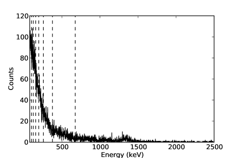
Binning the data into energy bins creates a vector of counts . We also have a background vector, , containing the observed background spectrum, binned in the same way. One energy bin is chosen as a reference bin (in this case, bin 1). The choice of reference bin is unimportant, as the anomaly statistic has been shown to be invariant to the choice of bin [10]. The spectral comparison ratios can then be computed by
| (1) |
for . Here and are the numbers of counts in the reference bin. This is mathematically equivalent to multiplying the vector by a spectral shape matrix :
| (2) |
| (3) |
There are linearly independent SCRs, since one bin is a reference bin. The SCR process compares against projections based on the ratio between bins in the background data and the counts in bin ; the deviations of the projections are given in the SCR vector . Since is computed using ratios between bins, it is insensitive to global changes in count rate unless they alter the spectral shape. This important feature allows for comparisons of spectra made with unequal observation times, which happens when numerous observations over wide areas are aggregated into spatial cells.
II-C2 Characterizing Expected Variation
To accurately detect anomalies, we first need to determine what variation can be expected in the natural background. First, we assume that counts in each energy bin follow an overdispersed Poisson distribution. As counts are aggregated across larger spatial cells, they become overdispersed; see Fig. 3. Consequently, we approximate that , where is the average variance-to-mean ratio of count rates ( for perfectly Poisson-distributed counts). is selected empirically by calculating the ratio for the area of interest. We know the relationship between the variance of random variables:
| (4) |
Hence, using (1) we may estimate :
| (5) |
Here is treated as an exact value rather than having its variance propagated. This is a significant simplification, as (1) is nonlinear in and an exact variance estimate could not be derived. Consequently, will be underestimated. The impact of this will be explored in Section IV.
The covariance would be best estimated from all previous background observations made in a spatial cell, so that . However, spatial mapping would be impractical if it required numerous repeated observations before detecting anomalies. The relationship between the covariance and the correlation is [11]:
| (6) |
To replace we must also rescale; may have resulted from an observation of a different duration than . Consequently, we can replace the covariance with a correlation:
| (7) |
where is the time taken to observe and the time taken to observe . This is obtained by replacing with , and likewise for , rescaling the observation to match the new observation time.
To compute we do not rely only on background observations made in the chosen spatial cell, as there is frequently not enough data to make this possible. Instead, is estimated from observations in all spatial cells by summing together observations into thirty-second intervals. The correlation between energy bins in these summed observations is easily computed.
Finally, we can construct the covariance matrix between energy bins in the SCR vector:
| (8) |
where is estimated by summing all observations across all spatial cells in the same way as for , then comparing each observation to the global mean spectrum to produce .
By using assumptions about the distribution of the data, we have avoided requiring direct calculation of from the data, as required by past SCR implementations, which would be impossible when there are too few background observations. To produce well-conditioned and invertible covariance matrices, many more observations than variables are required. This would require numerous repeated mapping passes before any anomalies can be detected, making the system impractical. Approaches based on shrinkage estimators are possible [12], but cannot work if there are only one or two observations.
The correlation matrices may be computed and reused for anomaly detection in all spatial cells; in very large regions where spectra vary greatly, the correlation matrices may be estimated separately for smaller areas within the monitored region. Any similar method using covariance matrices would require each spatial cell to contain observations of equal length, or require new covariance matrices to be computed for each spatial cell.
II-C3 Anomaly Detection
Previous work has developed a simple anomaly detection algorithm which makes use of the SCR vector [4]. In these applications a set of many independent background observations are made, and is calculated for each observation. After computing the covariance matrix for the resulting set of SCR vectors, is calculated for the new observation and it is compared to the background through the mathematical construct of the Mahalanobis distance:
| (9) |
The Mahalanobis distance measures the difference between a multivariate observation and the typical mean, normalizing by the typical variance expressed in the covariance matrix [11]. This implies that spectral shape changes consistent with already-observed natural background variations will cause only small increases in , while changes very different from the past data will produce large discrepancies.
If the estimated covariance matrix is accurate and the background radiation source is unchanging, the Mahalanobis distance should be -distributed with ) degrees of freedom [5]. In practice there are slight background fluctuations from various natural processes, and the distribution departs slightly from theoretical predictions [5]. (See Fig. 4.)
By setting a desired alarm threshold based on typical natural spectral variations, one can search for unusually large spectral anomalies, which may indicate source changes. To monitor a wide area, observations can be aggregated into spatial cells and the cumulative spectrum in each cell compared to previous observations. Each cell may contain different numbers of observations, and an individual cell may have observations at different times and locations from day to day.
Due to (7), as increases decreases. This renders the system more and more sensitive with longer observation times.
The method does not distinguish between equally-sized anomalies from natural or artificial sources, though the choice of energy bins may be made to optimize sensitivity to certain isotopes [4]. Additional benefits of this approach include being able to detect unexpected decreases in radioactivity as well as the replacement of one radioactive source with another, which may maintain a constant count rate in a given area while altering the spectral shape.
III Example Dataset
We collected a sample dataset between June 22nd and August 10th, 2012 at the University of Texas’s J. J. Pickle Research Campus. To survey the campus, the system was placed in a golf cart and driven on most work days on irregular routes. Total observation time amounted to twenty hours in 48 observation runs containing a total of more than 37,000 individual two-second observations.
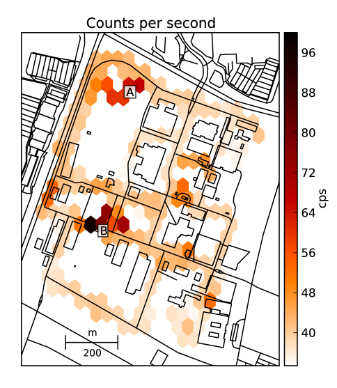
The natural gamma background varies spatially and temporally due to many natural factors. Our surveys revealed a spatially varying natural background across Pickle Research Campus. A map of average radiation levels over several weeks is shown in Fig. 2. Background activities vary spatially by a factor of two due to natural and artificial sources.
IV Analysis
IV-A Poisson Distribution Assumption
Our algorithmic approach relies on the underlying Poisson distribution of radiation data. To test the validity of this assumption, Poisson dispersion tests were performed on the dataset as a function of spatial scales. The Poisson dispersion test determines whether a given set of observations could plausibly have been drawn from the same Poisson distribution [13]. The test computes a dispersion parameter , defined by:
| (10) |
where is the mean of all observations and the total number of observations. This parameter is -distributed with degrees of freedom. Using this distribution, a value can be computed for , indicating the probability that the observed distribution of values would arise from a Poisson-distributed random variable. For example, dividing our dataset into 125-meter grid cells, we find that on average, , so we do not reject the hypothesis that the data are Poisson distributed; this falls to for 250-meter cells.
To quantify this, the index of dispersion was computed for all grid cells at various cell sizes. The index of dispersion is a measure of the variance of a distribution, compared to its mean:
| (11) |
where is the distribution’s mean and its variance. The variance of a Poisson distribution equals its mean, so the index of dispersion is expected to be one. Fig. 3 shows mean indices of dispersion for various grid cell sizes, demonstrating that smaller cells tend to have count rate distributions closer to the expected Poisson distribution, as expected. To account for this, we adjusted the dispersion parameter in Eq. 7 to match the mean index of dispersion for grid cells at a chosen spatial scale.
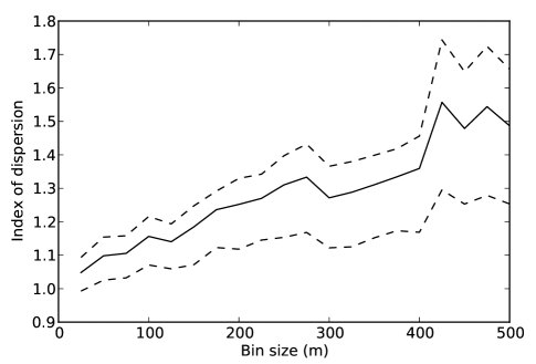
Of course, this problem is dependent on the nature of the area being mapped; areas with greater spectral variation on short spatial distances will need to be mapped with smaller spatial cells.
IV-B Comparing Spatial and Temporal Variation
Our dataset at the Pickle Research Campus revealed not only spatial but temporal variation in background. To compare the temporal variation to the spatial variation, the observation area was divided into grid cells 250 meters on each side, and each day’s set of observations was compared to two or more previous days using the SCRAM algorithm. Fig. 4 shows the distribution of recorded over several dozen passes through the area during July 2012. For comparison, it also plots the values calculated by comparing each grid cell’s spectrum to a fixed reference cell, rather than comparing it to the same cell on a previous day.
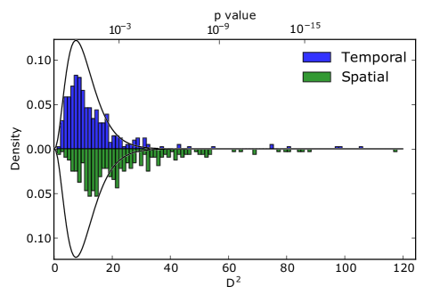
The spatial distribution is clearly shifted to the right, indicating that there is more spatial variance than temporal variance. This validates the assumption of the SCRAM method that it is best to compare spectral observations to previous observations made in the same place, rather than observations made at other locations. In other words, the background spectra vary much more spatially than they do temporally. This suggests that alarm thresholds may be set lower when using the SCRAM method to perform anomaly mapping, giving higher sensitivity without increased false alarm rates; knowledge of the prior background is more useful than the detector’s knowledge of what it observed thirty seconds ago at a different location, allowing more sensitive detection.
Further research should also investigate the impact of known natural variations in background radiation, such as those caused by rainfall’s interaction with radon daughter products, which have been extensively modeled [14]. At least five inches of rainfall occurred during our observation period, so these effects may be present in our example dataset, accounting for some of the temporal variance, and can be compared against existing models.
The presence of anomalies in Fig. 4 is not unusual. The -values are computed under the distribution, which the data do not follow perfectly: There are, of course, some true variations in natural background in the data, and the distribution of counts may be more or less overdispersed in different spatial cells. As noted in Section II-C2, estimates of are systematically low, making some observations appear more anomalous than they should. Also, some spectral comparisons were made with little data – because of irregular routes, a spatial cell may only contain a few seconds of data, giving an extremely poor estimate of the spectrum in that cell. Regardless of these issues, the algorithm is practical for anomaly detection, as demonstrated in the following simulations.
IV-C Detection Performance
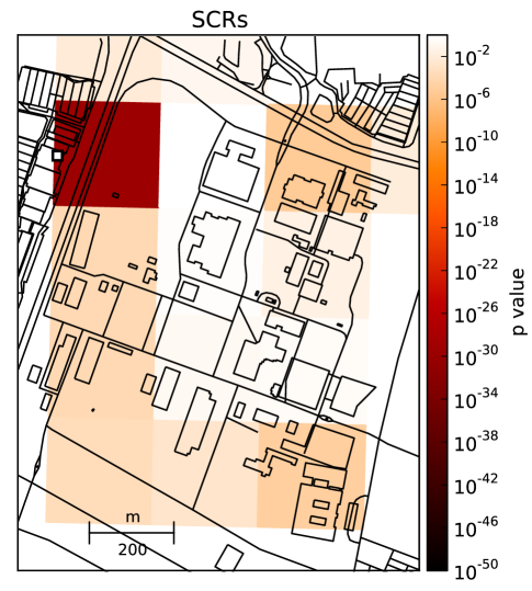
To demonstrate the expected performance of the SCRAM algorithm, we performed several simulations. Simulations used real observed spectra from a cesium-137 check source. The simulation code was calibrated by placing the source at known distances from the scintillator detector, and accounted for geometric attenuation of count rates, as well as the exponential attenuation due to gamma absorption in air.
The first simulation, shown in Fig. 5, injected a simulated 140 mCi cesium-137 source on the west side of Pickle Research Campus, 100 meters from the detector’s typical path. The detector, driving past at roughly 10 miles per hour, easily detected the source with (a far larger anomaly than any natural variation recorded in Fig. 4), demonstrating the ability of a small moving detector to detect sources at distance.
Next, we performed a simulation to calculate the minimum detectable radioactive source size at a variety of distances. We selected the same straight stretch of road on the northwest corner of the Pickle Research Campus and simulated the injection of a cesium-137 source at various distances from the road into the collected background data.
To choose our alarm threshold, we used the anomaly statistics distribution data shown in Fig. 4, selecting a threshold which only 1% of our example dataset exceeds. This corresponds to a 1% false alarm rate. For temporal comparisons of spectra, this threshold is , while for purely spatial comparisons the result is . We computed the minimum source size required to achieve a statistical power of 0.8 (that is, detection of a true positive at least 80% of the time) for both thresholds, and the results are given in Fig. 6.
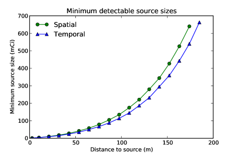
These results show that taking advantage of the exact prior background spectrum at each location leads to approximately 20% better detection performance over the use of spectra from a single fixed reference point. Of course, smaller sources would be detectable with a much larger scintillator or with a much longer observation time.
IV-D New and Improved?
There are many academic, prototype, and commercial systems that map radiation. The SCRAM system contains many elements in common with previous demonstrations, including the detector, GPS, spectral binning, spectral comparison algorithm, and spatial database. For these components, we are agnostic to replacements: different detectors or spectral binning choices could be chosen for specific applications. The novel component of the SCRAM system is estimation of the local background and its variance from previous observations. As has been pointed out previously, simply deploying larger detectors does not improve detection performance, as the local background is the limiting factor [15].
It is instructive to compare the SCRAM system against commercial systems and federal guidelines. However, these comparisons are difficult, given varying detector sizes and modes of operation. The Domestic Nuclear Detection Office has published testing methodologies we plan to follow as our system evolves from a proof-of-concept [16]. These guidelines require less than one false alarm per hour for 60-second integrations, amounting to a 1.7% false alarm rate. We chose a more strict limit of 1%, though this is not directly comparable; our spectral comparisons are made per spatial cell, rather than per 60-second integration. This limit can be chosen to meet user requirements.
For detection performance comparison, we can look to mapping systems with similar goals. The commercial ORTEC NaI-SS consists of a sodium iodide detector transported by car, recording spatial and spectral data every second [17]. For ORTEC’s chosen false alarm rate, the detector can identify a 10 Ci cesium-137 source at 3 meters while traveling at 10 miles per hour. Similarly, the SORIS coded aperture imager uses four large van-mounted sodium iodide plate scintillators, and can detect 1 mCi cesium-137 sources at a distance of 100 meters [3]. The detector in the SCRAM system is hundreds of times smaller; a simple scaling of our performance by collection area ignores many factors, but nevertheless, the SCRAM concept shows its relevance and promise by displaying significant gains over these previous detection limits when scaled to their detector sizes. Given all the differences in the systems, direct quantitative comparisons are not currently in order.
V Conclusion
In this work, we report on the development of an integrated system for wide-area radiation surveillance. A mobile detector is used to collect multiple-pass data, which is stored into a spatial-temporal spectral database. We developed a novel approach for anomaly detection of the spectral content by comparing observations to previous determinations of the background. Because the spatial variance is much larger than the temporal variance, this multi-pass methodology has the potential to deliver increased sensitivity to weak or distant sources, as demonstrated by simulations.
These developments are the first steps necessary to implement the larger vision of a providing continuous wide-area surveillance through the use of mobile sensors. Future improvements to the algorithm include the use of spatial kriging to improve estimates of background spectral shape, methods to determine optimal energy bin sizes, and adaptation for use in small, low-power mobile detectors.
Acknowledgment
The authors would like to thank T. Tipping of the Nuclear Engineering Teaching Laboratory and S. Pennington of Environmental Health and Safety at the University of Texas for their valuable suggestions and support, J. D. Biniaz and P. Vetter for their suggestions on the context and need for wide-area radiation surveillance, and staff at Bridgeport Instruments for technical support and advice regarding use of their detectors. The authors would also like to thank R. Schwitters for the suggestion to plot anomalies as values, as well as several other helpful suggestions.
References
- [1] P. Wasiolek, “An Aerial Radiological Survey of the City of North Las Vegas (Downtown) and the Las Vegas Motor Speedway,” Tech. Rep. DOE/NV/25946–352, Dec. 2007.
- [2] National Nuclear Security Administration, “Aerial Measuring System Factsheet.” http://www.nv.doe.gov/library/factsheets/AMS.pdf.
- [3] S. Zelakiewicz, R. Hoctor, A. Ivan, W. Ross, E. Nieters, W. Smith, D. McDevitt, M. Wittbrodt, and B. Milbrath, “SORIS—A standoff radiation imaging system,” Nuclear Instruments and Methods in Physics Research Section A, vol. 652, pp. 5–9, Oct. 2011.
- [4] D. M. Pfund, R. C. Runkle, K. K. Anderson, and K. D. Jarman, “Examination of Count-Starved Gamma Spectra Using the Method of Spectral Comparison Ratios,” IEEE Transactions on Nuclear Science, vol. 54, pp. 1232–1238, Aug. 2007.
- [5] D. M. Pfund, K. D. Jarman, B. D. Milbrath, S. D. Kiff, and D. E. Sidor, “Low Count Anomaly Detection at Large Standoff Distances,” IEEE Transactions on Nuclear Science, vol. 57, no. 1, pp. 309–316, 2010.
- [6] PostGIS Project, “PostGIS.” http://postgis.refractions.net/, 2012.
- [7] PostgreSQL Global Development Group, “PostgreSQL.” http://www.postgresql.org, 2012.
- [8] K. D. Jarman, R. C. Runkle, K. K. Anderson, and D. M. Pfund, “A comparison of simple algorithms for gamma-ray spectrometers in radioactive source search applications,” Applied Radiation and Isotopes, vol. 66, pp. 362–371, Mar. 2008.
- [9] W. Wei, Q. Du, and N. H. Younan, “Particle Swarm Optimization Based Spectral Transformation for Radioactive Material Detection and Classification,” in 2010 IEEE International Conference on Computational Intelligence for Measurement Systems and Applications (CIMSA), pp. 1–6, IEEE, 2010.
- [10] R. Runkle, M. Myjak, S. D. Kiff, and D. Sidor, “Lynx: An unattended sensor system for detection of gamma-ray and neutron emissions from special nuclear materials,” Nuclear Instruments and Methods in Physics Research A, vol. 598, pp. 815–825, 2009.
- [11] D. F. Morrison, Multivariate Statistical Methods. Duxbury, 4th ed., 2005.
- [12] M. J. Daniels and R. E. Kass, “Shrinkage Estimators for Covariance Matrices,” Biometrics, vol. 57, pp. 1173–1184, Dec. 2001.
- [13] C. R. Rao and I. M. Chakravarti, “Some small sample tests of significance for a Poisson distribution,” Biometrics, vol. 12, pp. 264–282, Sept. 1956.
- [14] J. F. Mercier, B. L. Tracy, R. d’Amours, F. Chagnon, I. Hoffman, E. P. Korpach, S. Johnson, and R. K. Ungar, “Increased environmental gamma-ray dose rate during precipitation: a strong correlation with contributing air mass,” Journal of Environmental Radioactivity, vol. 100, pp. 527–533, July 2009.
- [15] K. P. Ziock and W. H. Goldstein, “The Lost Source, Varying Backgrounds and Why Bigger May Not Be Better,” in Unattended Radiation Sensor Systems for Remote Applications, pp. 60–70, AIP, 2002.
- [16] Domestic Nuclear Detection Office, “Technical Capability Standard for Vehicle Mounted Mobile Systems,” Tech. Rep. 500-DNDO-119420v0.00, Aug. 2013.
- [17] ORTEC, “NaI-SS Radiation Search System.” http://www.ortec-online.com/download/nai-ss-radiation-search-system.pdf, 2013.