IGM Constraints from the SDSS-III/BOSS DR9
Ly Forest Transmission Probability Distribution Function
Abstract
The Ly forest transmission probability distribution function (PDF) is an established probe of the intergalactic medium (IGM) astrophysics, especially the temperature-density relationship of the IGM. We measure the transmission PDF from 3393 Baryon Oscillations Spectroscopic Survey (BOSS) quasars from SDSS Data Release 9, and compare with mock spectra that include careful modeling of the noise, continuum, and astrophysical uncertainties. The BOSS transmission PDFs, measured at , are compared with PDFs created from mock spectra drawn from a suite of hydrodynamical simulations that sample the IGM temperature-density relationship, , and temperature at mean-density, , where . We find that a significant population of partial Lyman-limit systems with a column-density distribution slope of are required to explain the data at the low-transmission end of transmission PDF, while uncertainties in the mean Ly forest transmission affect the high-transmission end. After modelling the LLSs and marginalizing over mean-transmission uncertainties, we find that best describes the data over our entire redshift range, although constraints on are affected by systematic uncertainties. Within our model framework, isothermal or inverted temperature-density relationships () are disfavored at a significance of over 4, although this could be somewhat weakened by cosmological and astrophysical uncertainties that we did not model.
Subject headings:
intergalactic medium — quasars: emission lines — quasars: absorption lines — methods: data analysis1. Introduction
Remarkably soon after the discovery of the first high-redshift () quasars (Schmidt 1965), Gunn & Peterson (1965) realized that the amount of resonant Lyman- (Ly) scattering off neutral hydrogen structures observed in the spectra of these quasars could be used to constrain the state of the inter-galactic medium (IGM) at high-redshifts: they deduced that the hydrogen in the inter-galactic medium had to be highly photo-ionized (neutral fractions of ) and hot (temperatures, ).
Lynds (1971) then discovered that this Ly absorption could be separated into discrete absorption lines, i.e. the Ly “forest”. Over the next two decades, it was recognized that the individual Ly forest lines have Voigt absorption profiles corresponding to Doppler-broadened systems with (see, e.g., Rauch et al. 1992; Ricotti et al. 2000; Schaye et al. 2000; McDonald et al. 2001; Tytler et al. 2004; Lidz et al. 2010; Becker et al. 2011) and neutral column densities of (Petitjean et al. 1993; Penton et al. 2000; Janknecht et al. 2006; Rudie et al. 2013), and increasingly precise measurements of mean Ly forest transmission have been carried out (Theuns et al. 2002; Bernardi et al. 2003; Faucher-Giguère et al. 2008; Becker et al. 2013). However, the exact physical nature of these absorbers was unclear for many years (see Rauch 1998, for a historical review of the field).
Beginning in the 1990s, detailed hydrodynamical simulations of the intergalactic medium led to the current physical picture of the Ly forest arising from baryons in the IGM which trace fluctuations in the dark matter field induced by gravitational collapse, in ionization balance with a uniform ultraviolet ionizing background (see, e.g., Cen et al. 1994; Miralda-Escudé et al. 1996; Croft et al. 1998; Davé et al. 1999; Theuns et al. 1998). A physically-motivated analytic description of this picture is the fluctuating Gunn-Peterson approximation (FGPA, Croft et al. 1998; Hui et al. 1997), in which the Ly optical depth, , scales with underlying matter density, , through a polynomial relationship:
| (1) |
where is the background photoionization rate, and is the matter density relative to the mean density of the universe at the given epoch. In the second proportionality above, we have made the assumption that the local temperature of the gas has a polynomial relationship with the local density,
| (2) |
where is the gas temperature at mean-density and parametrizes the temperature-density relation, which encodes the thermal history of the IGM (e.g., Hui & Gnedin 1997, Schaye et al. 1999, Ricotti et al. 2000, McDonald et al. 2001, Hui & Haiman 2003; see Meiksin 2009 for a detailed overview on the relevant physics).
Over the the past decade-and-a-half, the 2000-2008 Sloan Digital Sky Survey (SDSS-I and -II, York et al. 2000; Stoughton et al. 2002, http://www.sdss.org) spectroscopic data has represented a dramatic improvement in the statistical power available to Ly forest studies: McDonald et al. (2006) measured the 1-dimensional Ly forest transmission power spectrum from SDSS quasar sightlines. This measurement was used to place significant constraints on cosmological parameters and large-scale structure (see, e.g., McDonald et al. 2005b; Seljak et al. 2005; Viel & Haehnelt 2006).
The McDonald et al. (2006) quasar sample, which in its time represented a increase in sample size over previous data sets, is superseded by the Baryon Oscillations Sky Survey (BOSS, part of SDSS-III; Eisenstein et al. 2011; Dawson et al. 2013) quasar survey. This spectroscopic survey, which operated between fall 2009 and spring 2014, is aimed at taking spectra of quasars (Dawson et al. 2013) with the goal of constraining dark energy at using transverse correlations of Ly forest absorption (see, e.g., Slosar et al. 2011) to measure the baryon acoustic oscillation (BAO) scale111There is also a simultaneous effort to observe million luminous red galaxies, to measure the BAO at . See, e.g., Anderson et al. (2014). . At time of writing, the full BOSS survey is complete, with high-redshift quasars observed, although this paper is based on the earlier sample of BOSS quasars from SDSS Data Release 9 (DR9 Ahn et al. 2012; Pâris et al. 2012; Lee et al. 2013).
The quality of the individual BOSS Ly forest spectra might appear at first glance inadequate for studying the astrophysics of the IGM, that have to-date been carried out largely with high-resolution, high-S/N spectra: the typical BOSS spectrum has per pixel222All spectral signal-to-noise ratios quoted in this paper are per SDSS/BOSS pixel unless noted otherwise , since the BAO analysis is optimized with large numbers of low signal-to-noise-ratio sightlines, densely-sampled on the sky (McDonald & Eisenstein 2007; McQuinn & White 2011). It is therefore interesting to ask whether it is possible to model the various instrumental and astrophysical effects seen in the BOSS Ly forest spectra, to sufficient accuracy level to exploit the unprecedented statistical power.
In this paper, we will measure the probability distribution function (PDF) of the Ly forest transmission, , from BOSS. This one-point statistic, which was first studied by Jenkins & Ostriker (1991), is sensitive to astrophysical parameters such as the amplitude of matter fluctuations and the thermal history of the IGM. However, the transmission333The Ly forest transmitted flux fraction is sometimes also referred to as ’flux’ in the literature; but we do however use the variable to refer to this quantity. PDF is also highly sensitive to effects such as pixel noise level, resolution of the spectra, and systematic uncertainties in the placement of the quasar continuum level, especially in moderate resolution spectra such as SDSS or BOSS. Desjacques et al. (2007) studied the transmission PDF from a sample of Ly forest spectra from SDSS Data Release 3 (Abazajian et al. 2005). Using mock spectra generated from a log-normal model of the Ly forest with parameters tuned to reproduce high-resolution, high- spectra, they fitted for the estimated pipeline noise level and continuum-fitting errors in the SDSS spectra. They concluded that the noise levels reported by the SDSS pipeline were underestimated by , consistent with the findings of McDonald et al. (2006). They also found that the quasar continuum-level was systematically lower by in comparison with a power-law extrapolated from redwards of the quasar Ly line, with a RMS variance of , although certain aspects of their study, e.g., the noise modelling and quasar continuum model, were rather crude.
We intend to take an approach distrinct from that of Desjacques et al. (2007): instead of treating the noise and continuum as free parameters, we will attempt to measure the BOSS Ly forest transmission PDF using a rigorous treatment of the noise and continuum-fitting, and then adopt a “forward-modeling” approach of trying to model the various instrumental effects as accurately as possible in mock spectra generated from detailed hydrodynamical simulations. Using the raw individual exposures and calibration data from BOSS, we will first implement a novel probabilistic method for co-adding the exposures, which will yield more accurate noise estimates as well as enable self-consistent noise modelling in mock spectra. Similarly, we will use a new method for continuum estimation called mean-flux regulated/principal component analysis (MF-PCA; Lee et al. 2012). This technique provides unprecedented continuum accuracy for noisy Ly forest spectra: RMS errors for and RMS errors for spectra.
On the modeling side, we will use the detailed hydrodynamical IGM simulations of Viel et al. (2013a) as a basis. The mock spectra are then smoothed to BOSS resolution, have Lyman-limit systems (LLS) and metal contamination added, followed by the introduction of pixel noise based on our improved noise estimates. We will then self-consistently introduce continuum errors by applying our continuum-estimation procedure on the mock spectra.
With the increase in statistical power from the sheer number of BOSS spectra, and our improved modeling of the noise and continuum, we expect to significantly reduce the errors on the measured transmission PDF in comparison with Desjacques et al. (2007). This should enable us to place independent constraints on the shape of the underlying transmission PDF, and the thermal history of IGM as parametrized by the power-law temperature-density relation, and .
The IGM temperature-density relationship is a topic of recent interest, as Bolton et al. (2008) and Viel et al. (2009) have found evidence of an inverted temperature-density relation, , implying that voids are hotter than overdensities, the IGM at from the transmission PDF from high-resolution, high- Ly forest spectra (Kim et al. 2007). This result is in contrast with theoretical expectations of (Miralda-Escudé & Rees 1994; Hui & Gnedin 1997; Theuns et al. 1998; Hui & Haiman 2003), which arises from the balance between adiabatic cooling in the lower-density IGM and photoheating in the higher-density regions. Even inhomogeneous He II reionization, which is expected to flatten the IGM temperature-density relation (see, e.g., Furlanetto & Oh 2008; Bolton et al. 2009; McQuinn et al. 2009), is insufficient to account for the extremely low values of estimated by the aforementioned authors (although inversions could occur at higher densites, see, e.g., Meiksin & Tittley 2012).
Indeed, earlier papers studying the temperature-density relationship using either the transmission PDF (McDonald et al. 2001) or by measuring the Doppler parameters and hydrogen column densities of individual forest absorbers (the so-called relation, e.g., Schaye et al. 1999; Ricotti et al. 2000; Rudie et al. 2012) have found no evidence of an inverted . In recent years, the decay of blazar gamma rays via plasma instabilities (Broderick et al. 2012, Chang et al. 2012; although see Sironi & Giannios 2014) has been invoked as a possible mechanism to supply the heat necessary to flatten to the observed levels (Puchwein et al. 2012).
It would be desirable to perform an independent re-analysis of high-resolution data taking into account continuum-fitting bias (Lee 2012), to place these claims on a firmer footing. However, Lee & Spergel (2011) have argued that the complete SDSS DR7 (Abazajian et al. 2009) Ly forest data set could have sufficient statistical power to place interesting constraints on , even assuming continuum-fitting errors at the RMS level. Therefore, with the current BOSS data, we hope to model noise and resolution, as well as astrophysical systematics, at a sufficient precision to place interesting constraints on the IGM thermal history.
This paper is organized as follows: we first give a broad overview of the BOSS Ly forest data set, followed by our measurement of the BOSS transmission PDF with detailed descriptions of our method of combining multiple raw exposures and continuum estimation. We then discuss how we include various instrumental and astrophysical effects into our modeling of the transmission PDF starting with hydrodynamical simulations. The model transmission PDF is then compared with the observed PDF to obtain constraints on the thermal parameters governing the IGM.
2. Data
2.1. Summary of BOSS
BOSS (Dawson et al. 2013) is part of SDSS-III (Eisenstein et al. 2011; the other surveys are SEGUE-2, MARVELS, and APOGEE). The primary goal of the survey is to carry out precision baryon acoustic oscillations at and , from the luminous red galaxy distribution and Ly forest absorption field, respectively (see, e.g., Anderson et al. 2014; Busca et al. 2013; Slosar et al. 2013). Its eventual goal is to obtain spectra of million luminous red galaxies and quasars over 4.5 years of operation.
BOSS is conducted on upgraded versions of the twin SDSS spectrographs (Smee et al. 2013) mounted on the 2.5m Sloan telescope (Gunn et al. 2006) at Apache Point Observatory, New Mexico. One thousand optical fibers mounted on a plug-plate at the focal plane (spanning a field of view) feed the incoming flux to the two identical spectrographs, of which 160-200 fibers per plate are allocated to quasar targets (see Ross et al. 2012; Bovy et al. 2011, for a detailed description of the quasar target selection). Both spectrographs split the light into a blue and red camera that cover , with the dichroic overlap region occurring at around . The resolving power ranges from 1300 at the blue end to the 2600 at the red end.
Each plate is observed for sufficiently long to achieve the S/N requirements set by the survey goals; typically, 5 individual exposures of 15 minutes are taken.The data are processed, calibrated, and combined into co-added spectra by the “idlspec2d” pipeline, followed by a pipeline which operates on the 1D spectra to classify objects and assign redshifts (Bolton et al. 2012). However, as described later in this paper, we will generate our own co-added spectra from the individual exposures and other intermediate data products.
2.2. Data Cuts
In this paper we use data from the publicly-available SDSS Data Release 9 (DR9 Ahn et al. 2012). This includes 87,822 quasars at all redshifts, that have been confirmed by visual inspection as described in Pâris et al. (2012). In Lee et al. (2013), we have defined a further subset of 54,468 quasars with that are suitable for Ly forest analysis, and have provided in individual FITS files for each quasar various products such as sky masks, masks for damped Ly absorbers (DLAs), noise corrections, and continua; these are designed to ameliorate systematics in the BOSS spectra and aid in Ly forest analysis (see Table 1 in Lee et al. 2013 for a full listing). While we use this Lee et al. (2013) catalog as a starting point, in this paper we will generate our own custom co-added spectra and noise estimates.
The typical signal-to-noise ratio of the BOSS Ly forest quasars is low: per pixel within the Ly forest; this criterion is driven by a strategy to ensure a large number of sightlines over a large area in order to optimize the 3D Ly forest BAO analysis. (McDonald & Eisenstein 2007; McQuinn & White 2011), rather than increasing the S/N in individual spectra. However, for our analysis we wish to select a subset of BOSS Ly forest sightlines with reasonably high S/N in order to reduce the sensitivity of our PDF measurement to inaccuracies in our modeling of the noise and continuum of the BOSS spectra. We therefore make a cut on S/N, including only sightlines that have a median per pixel within the Ly forest444Defined as the region in the quasar restframe, defined with respect to the pipeline noise estimate (see Lee et al. 2013) — this selects only of the spectra with the highest S/N. The Ly forest region of each quasar must also include at least 30 pixels () within one of our absorption redshift bins of , , and , with bin widths of (see § 3.3).
We discard spectra with identified DLAs in the sightline, as listed in the ‘DLA Concordance Catalog’ used in the Lee et al. (2013) sample. This DLA catalog (W. Carithers 2014, in prep.) includes objects with column densities ; however, the completeness of this catalog is uncertain below . We therefore discard only sightlines containing DLAs with , and take into account lower column-density absorbers in our subsequent modelling of mock spectra. At the relatively high S/N that we will work with (see below), the detection efficiency of DLAs is essentially 100% (see, e.g., Prochaska et al. 2005; Noterdaeme et al. 2012) and thus we expect our rejection of DLAs to be quite thorough.
Measurements of the Ly forest transmission PDF are known to be sensitive to the continuum estimate (Lee 2012),
but in this paper we use an automated continuum-fitter, MF-PCA (Lee 2012), that is less susceptible to biases introduced by manual continuum
estimation. Moreover, unlike the laborious process of manually-fitting continua on high-resolution spectra, the automated
continuum estimation can be used to explore various biases in continuum estimation.
For this purpose, we will use the same MF-PCA continuum estimation used in Lee et al. (2013),
albeit with minor modifications as described in § 3.2.
We select only quasars that appear to be well-described
by the continuum basis templates, based on the goodness-of-fit to the quasar spectrum redwards of Ly.
This is flagged by the variable CONT_FLAG as listed
in the Lee et al. (2013) catalog (see Table 3 in that paper).
Broad Absorption Line (BAL) quasars, which are difficult to estimate continua due to broad intrinsic
absorption troughs, have already been discarded from the Lee et al. (2013) sample.
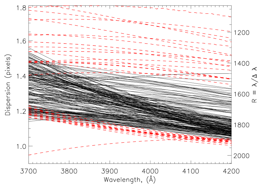
Another consideration is that the shape of the transmission PDF is affected by the resolution of the spectrum, especially since the BOSS spectrographs do not resolve the Ly forest. The exact spectral resolution of a BOSS spectrum at a given wavelength varies as a function of both observing conditions and row position on the BOSS CCDs. The BOSS pipeline reports the wavelength dispersion at each pixel, , in units of the co-added wavelength pixel size (binned such that ). This is related to the resolving power by . Palanque-Delabrouille et al. (2013) have recently found, using their own analysis of the width of the arc-lamp lines and bright sky emission lines, that the spectral dispersion reported by the pipeline had a bias that depended on the CCD row and increased with wavelength, up to 10% at . We will correct for this bias when creating mock spectra to compare with the data, as described in § 4. Figure 1 shows the (uncorrected) pixel dispersions from 236 BOSS quasars from the , bin, as a function of wavelength at the blue end () of the spectrograph. At fixed wavelength, there are outliers that contribute to the large spread in , e.g., ranging from at . We therefore discard spectra with outlying values of based on the following criterion: we first rank-order the spectra based on their value evaluated at the central wavelength of each PDF bin (i.e. at ), and then discarded spectra below the 5th percentile and above the 90th percentile. This is illustrated by the red-dashed lines in Figure 1.
Finally, since our noise estimation procedure uses the individual BOSS exposures, we discard objects that have less than three individual exposures available.
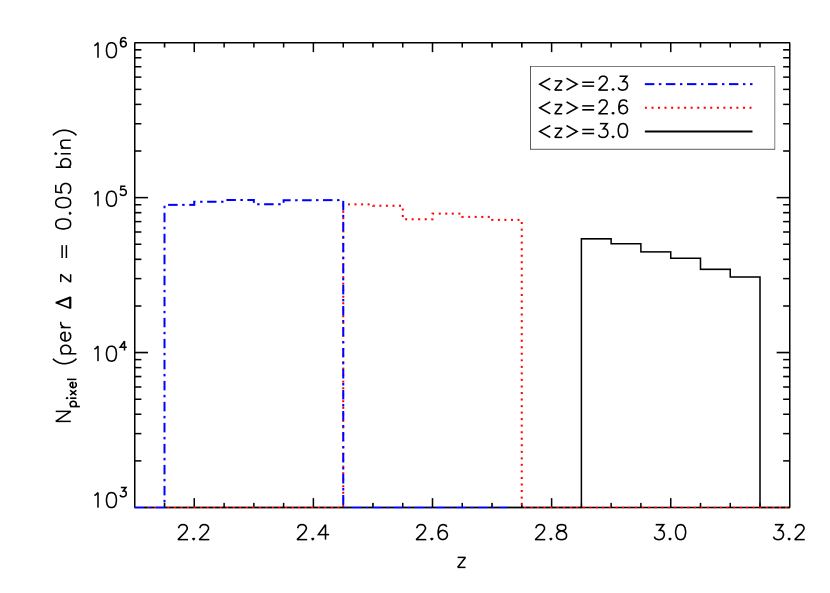
Our final data set comprises 3373 unique quasars with redshifts ranging from to , and a median S/N of per pixel. This data set represents only a small subsample of the BOSS DR9 quasar spectra, but is over two orders-of-magnitude larger than high-resolution quasar samples previously used for transmission PDF analysis. Table 1 summarizes our data sample, and the statistics of the redshifts and S/N bins for which we measure the transmission PDF. Figure 2 shows histograms of the pixels used in our analysis, as a function of absorption redshift.
| Ly Forest | aaMedian S/N within Ly forest. | bbNumber of contributing spectra. | ccNumber of pixels. | ddVelocity path length. | eeRedshift path length. | ffAbsorption distance, where . For this conversion, we assume and . |
|---|---|---|---|---|---|---|
| Redshift | (per pixel) | () | ||||
| 6-8 | 1109 | 288442 | 219 | 704 | ||
| 8-10 | 501 | 129141 | 97.9 | 315 | ||
| 561 | 146478 | 111 | 357 | |||
| 6-8 | 1004 | 229898 | 191 | 646 | ||
| 8-10 | 490 | 107001 | 88.6 | 300 | ||
| 604 | 140843 | 117 | 396 | |||
| 6-8 | 511 | 108443 | 99.7 | 358 | ||
| 8-10 | 326 | 72448 | 66.7 | 239 | ||
| 341 | 74284 | 68.3 | 245 |
3. Measuring the transmission PDF from BOSS
In this section, we will measure the Ly forest transmission PDF from BOSS. In principle, the transmission PDF is simply the histogram of the transmitted flux in the Ly forest after dividing by the quasar continuum. However, with the comparatively noisy BOSS data we need to ensure an accurate estimate of the pixel noise. We will therefore first describe a new probabilistic method for co-adding the individual BOSS exposures that will enable us to have an accurate noise estimate. We will also describe the continuum-estimation method with which we normalize the forest transmission.
3.1. Co-addition of Multiple Exposures and Noise Estimation
Since we intend to model BOSS spectra with modest S/N, we need an accurate estimate of the pixel noise that also allows us to separate out the contributions from Poisson noise due to the background and sky as well as read noise from the the detector. In this subsection, we will construct an accurate probabilistic model of the flux and noise of the BOSS spectrograph, based on the individual exposure data that BOSS delivers.
The basic BOSS spectral data consists of a spectrum of each raw exposure, (inclusive of noise), an estimate of the sky , and a calibration vector , where indicates the exposure of the exposures taken555Typically there are exposures of 15 minutes each, although this can vary due to the requirements to achieve a given over each individual plug-plate, as determined by the overall BOSS survey strategy (see Dawson et al. 2013).. The quantity is the actual sky model that was subtracted from the fiber spectra in the extraction. The calibration vector is defined as , with being the flux of exposure in units of photoelectrons. The idlspec2d pipeline then estimates the co-added spectrum of the true object flux, , from the raw individual exposures, sky estimates, and calibration vectors.
The BOSS data reduction pipeline also delivers noise estimates in the form of variance vectors, which are however known to be inaccurate (McDonald et al. 2006; Desjacques et al. 2007; Lee et al. 2013; Palanque-Delabrouille et al. 2013).
To quantify the fidelity of the BOSS noise estimate, we used the so-called ‘side-band’ method described in Lee et al. (2014a) and Palanque-Delabrouille et al. (2013), which uses the variance in flat, absorption-free, regions of the quasar spectra to quantify the fidelity of the noise estimate. First, we randomly selected 10,000 BOSS quasars (omitting BAL quasars) from the Pâris et al. (2012) catalog in the redshift range , evenly distributed into 20 redshift bins of width (i.e., 500 objects per bin). We then consider the flat spectral region in the quasar restframe, which is dominated by the smooth power-law continuum and relatively unaffected by broad emission lines (e.g., Vanden Berk et al. 2001; Suzuki 2006) or absorption lines. The pixel variance in this flat portion of the spectrum should therefore be dominated by spectral noise, allowing us to examine whether the noise estimate provided by the pipeline is accurate. We then evaluate the ratio of, , the pixel flux RMS in the restframe region divided by the average pipeline noise estimate, :
| (3) |
where the summations and average flux is evaluated in the quasar restframe .
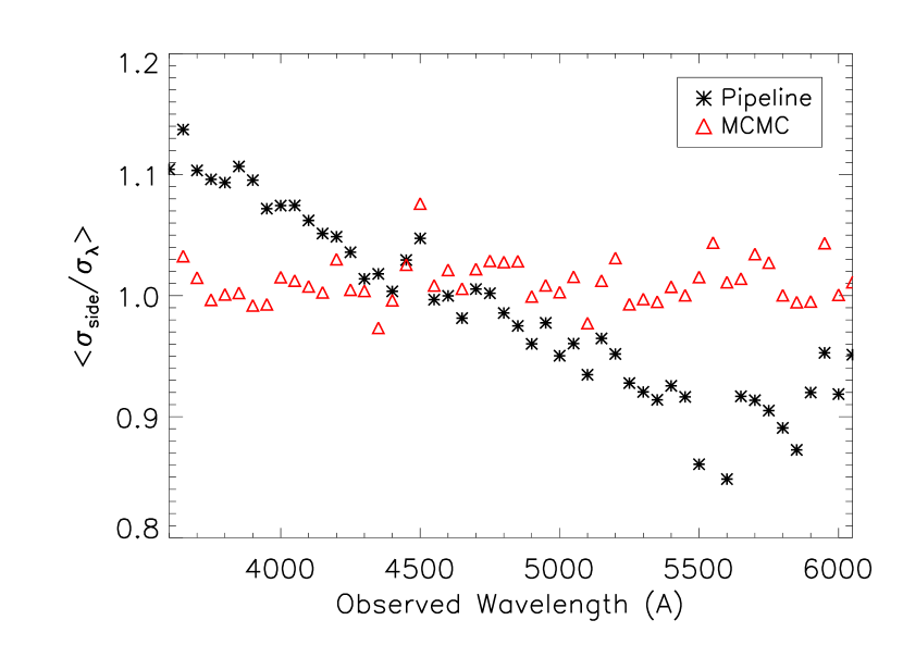
In Figure 3, this quantity is averaged over the 500 individual quasars per redshift bin and plotted as a function of the observed wavelength corresponding to . With a perfect noise estimate, should be unity at all wavelengths, but we see that the BOSS pipeline underestimates the true noise in the spectra at , by up to at the blue end of the spectra, with an overall tilt that changes over to an overestimate at . Lee et al. (2013) and Palanque-Delabrouille et al. (2013) provide a set of correction vectors that can be applied to the pipeline noise estimates to bring the latter to within several percent of the true noise level across the wavelength coverage of the blue spectrograph.
Unfortunately, these noise corrections are inadequate for our purposes, since we want to generate realistic mock spectra that have different realizations of the Ly forest transmission field from the actual spectra, i.e., a different . We therefore require a method that not only accurately estimates the noise in a given BOSS spectrum, but also separates out the photon-counting and CCD terms in the variance, that results from applying the Horne (1986) optimal spectral extraction algorithm:
| (4) |
where is the CCD read-noise.
To resolve this issue, we apply our own novel statistical method to the individual BOSS exposures to generate co-added spectra while simultaneously estimating the corresponding noise parameters for each individual spectrum. This procedure, which uses a Gibbs-sampled Markov-Chain Monte Carlo (MCMC) algorithm, is described in detail in the Appendix. Initially, we attempted to model the noise with just a single constant noise parameter which rescales the read-noise term of Equation 4, but this was found to be inadequate. This is likely because an optimal extraction algorithm weights by the product of the S/N and object profile, causing the corresponding variance to have a non-linear dependence on the flux and sky level. Furthermore, systematic errors in the reduction, sky-subtraction and calibration will result in additional noise contributions which could depend on sky level, object flux, or wavelength, hence deviating from this simple model.
After considerable trial-and-error to find a model that best minimizes the bias illustrated in Figure 3, we settled on the form:
| (5) |
where
| (6) |
where the are free parameters in our noise model, while the factor in the 2nd term (the pixel dispersion) provides a rough approximation for the wavelength-dependence of the spot-size (i.e. the size of the raw CCD image in the spatial direction). Meanwhile, is the average CCD read-noise per wavelength bin in the BOSS spectra (D.J. Schlegel et al., in preparation). The quantities , , and (sky flux, calibration vector, and dispersion, respectively) are taken directly from the BOSS pipeline.
In addition, we assume that the pixel noise can be modeled as a Gaussian distribution with a variance given by Equation 5. The first, photon counting, term in the equation should formally be modeled as a Poisson distribution, but since the BOSS spectrograph always receives counts even at the blue end of the spectrograph where the counts are the lowest, it is reasonable to use the Gaussian approximation because even in the limit of low S/N (i.e. when the spectrum is dominated by the sky flux), the moderate resolution ensures that there are at least several dozen sky photons per pixel in each exposure.
For each BOSS spectrum, we use the MCMC procedure described in the Appendix to combine the multiple exposures while simultaneously estimating the noise parameters and true observed spectrum, . With the optimal estimates of and for a given spectrum, the estimated noise variance is then simply Equation 5.
An important advantage of the form in Equation 5 is that the object photon noise is explicitly separated out. This facilitates the construction of a mock spectrum with the same noise characteristics as a true spectrum, but with a different spectral flux. For example, a mock spectrum of the Ly forest will have a very different transmission field than the original data, and so the variance due to object photon counting noise can be added appropriately, in addition to contributions from the known sky, and the read noise term (Equation 5). Our empirical determination of the parameters govering this noise model for each individual spectrum form a crucial ingredient in our forward model, which we will describe in § 4.
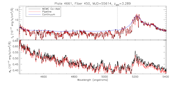
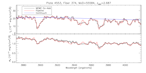
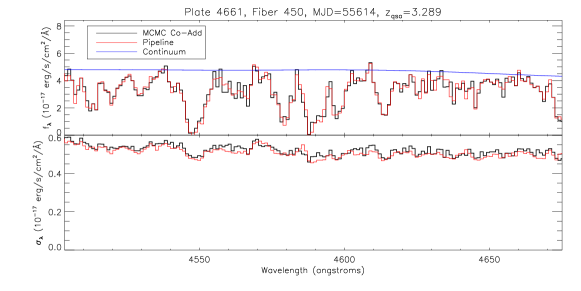
Our MCMC procedure works for spectra from a single camera, either red or blue; we have not yet generalized it to combine blue and red spectra of each object. However, the spectral range of the blue camera alone () covers the Ly forest up to , i.e., most practical redshifts for Ly forest analysis. For the purposes of this paper, we restrict ourselves to spectra from the blue camera alone.
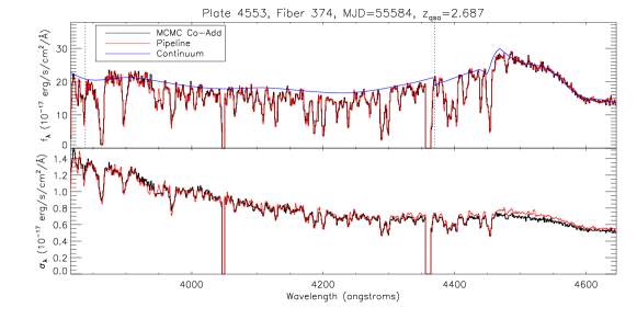
In Figures 4 and 5, we show examples of co-added BOSS quasar spectra, using both the MCMC procedure and the standard BOSS pipeline. In the upper panels, the MCMC co-adds are not noticeably different from the BOSS pipeline, although the numerical values are different. In the lower panels, we show the estimated noise from both methods — the differences are larger than in the fluxes but still difficult to distinguish by eye.
We therefore return to the statistical analysis by calculating , the ratio of the pixel variance against the estimated noise from the flat region of BOSS quasars; this ratio, computed for our MCMC coadds, is plotted in Figure 3. With these new co-adds, we see that this ratio is within roughly of unity across the entire wavelength range relevant to our subsequent analysis, with an overall bias of (i.e. the noise is still underestimated by this level). Crucially, we have removed the strong wavelength dependence of that was present in the standard pipeline, and we suspect most of the scatter about unity is caused by the limited number of quasars (500 per bin) available for this estimate, which will be mitigated by the larger number of quasars spectra available in the subsequent BOSS data releases. In principle, we could correct the remaining noise bias, but since our selected spectra have , this remaining noise bias would smooth the forest transmission PDF by an amount roughly of the average PDF bin width (). As we shall see, there are other systematic uncertainties in our modeling that have much larger effects than this, therefore we regard our noise estimates as adequate for the subsequent transmission PDF analysis, without requiring any further correction.
3.2. Mean-Flux Regulated Continuum Estimation
In order to obtain the transmitted flux of the Ly forest666Note that the ideal/model observed flux described in the noise modelling section, , and the Ly forest transmission , are completely different quantities. we first need to divide the observed flux, , by an estimate for the quasar continuum, . We use the version of mean-flux regulated/principal component analysis (MF-PCA) continuum fitting (Lee et al. 2012) described in Lee et al. (2013). Initially, PCA fitting with 8 eigenvectors is performed on each quasar spectrum redwards of the Ly line () in order to obtain a prediction for the continuum shape in the Ly forest region (e.g., Suzuki et al. 2005). The slope and amplitude of this initial continuum estimate is then corrected to agree with the Ly forest mean transmission, , at the corresponding absorber redshifts, using a linear correction function.
The only difference in our continuum-fitting with that in Lee et al. (2013) is that here we use the latest mean-flux measurements of Becker et al. (2013) to constrain our continua. Their final result yielded the power-law redshift evolution of the effective optical depth in the unshielded Ly forest, defined in their paper (although they only removed contributions from absorbers). This is given by
| (7) |
with best-fit values of at .
However, the actual raw measurement made by Becker et al. (2013) is the effective total absorption within the Ly forest region of their quasars, which also contain contributions from metals and optically-thick systems:
| (8) |
where and denote the IGM optical depth contributions from metals and Lyman-limit systems, respectively. For the purposes of our continuum-fitting, the quantity we require is , since the and contributions are also present in our BOSS spectra. Becker et al. (2013) did not publish their raw , therefore we must now ‘uncorrect’ the metal and LLS contributions from the published . The discussion below therefore attempts to retrace their footsteps and does not necessarily reflect our own beliefs regarding the actual level of these contributions.
We find by simply averaging over the Schaye et al. (2003) metal correction tabulated by Faucher-Giguère et al. (2008) (i.e., the values in bins from their Table 4), that were used by Becker et al. (2013) to normalize their relative mean-flux measurements. Note that there is no redshift dependence on in this context, because Becker et al. (2013) argued that the metal contribution does not vary significantly over their redshift range. Whether or not this is really true is unimportant to us at the moment, since we are merely ‘uncorrecting’ their measurement.
The LLS contribution to the optical depth is re-introduced by integrating over , the column-density distribution of neutral hydrogen absorbers:
| (9) | |||||
where is the Doppler parameter and is the rest-frame equivalent width (we use the analytic approximation given by Draine 2011, valid in the saturated regime).
Following Becker et al. (2013), we adopted a fixed value of and assumed that , where is given by the broken power-law column density distribution of Prochaska et al. (2010) and . Becker et al. (2013) had corrected for super-LLSs and DLAs in the column-density range , but as discussed above we have discarded all sightlines that include DLAs, therefore we reintroduce the optical depth contribution for super-LLSs, i.e., . We find . This is a small correction, giving rise to only a change in at .
This estimate of the raw absorption, , is now the constraint used to fit the continua of the BOSS quasars, i.e. we set . Note that in our subsequent modelling of the data, we will use the same to fit the mock spectra to ensure an equal treatment between data and mocks. Since includes a contribution from optically-thick systems, our mock spectra will need to account for these systems as we shall describe in .
The MF-PCA technique requires spectral coverage in the quasar restframe interval . However, as noted in the previous section, we work with co-added BOSS spectra from only the blue cameras covering ; this covers the full interval required for the PCA fitting only for quasars. However, the differences in the fluxes between our MCMC co-adds and the BOSS pipeline co-adds are relatively small, and we do not expect the relative shape of the quasar spectrum to vary significantly. We can thus carry out PCA fitting on the BOSS pipeline co-adds, which cover the full observed range (), to predict the overall quasar continuum shape. This initial prediction is then used to perform mean-flux regulation using the MCMC co-adds and noise estimates, to fine-tune the amplitude of the continuum fits.
The observed flux, , is divided by the continuum estimate, , to derive the Ly forest transmission, . For each quasar, we define the Ly forest as the rest wavelength interval . This wavelength range conservatively avoids the quasar’s Ly/O VI emission line blend by on the blue end, as well as the proximity zone close to the quasar redshift by staying from the nominal quasar systemic redshift. We are now in a position to measure the transmission PDF, which is simply the histogram of pixel transmissions .
3.3. Observed transmission PDF from BOSS
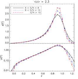
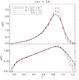
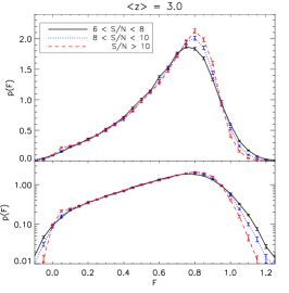
Since the Ly forest evolves as a function of redshift, we measure the BOSS Ly forest transmission PDF in three bins with mean redshifts of , , and , and bin sizes of . These redshifts bins were chosen to match the simulations outputs (§ 4.1) that we will later use to make mock spectra to compare with the observed PDF; this choice of binning leads to the gap at as seen in Figure 2. In this paper, we restrict ourselves to since the primary purpose is to develop the machinery to model the BOSS spectra. In subsequent papers, we will apply these techniques to analyze the transmission PDF in the full range using the larger samples of subsequent BOSS data releases (DR10, Ahn et al. 2014).
Another consideration is that the transmission PDF is strongly affected by the noise in the data. While we will model this effect in detail (§ 4), there is a large distribution of S/N within our subsample ranging from per pixel to per pixel. We therefore further divide the sample into three bins depending on the median S/N per pixel within the Ly forest: , , . The consistency of our results across the S/N bins will act as an important check for the robustness of our noise model (§ 3.1).
We now have nine redshift and S/N bins in which we evaluate the transmission PDF from BOSS; the sample sizes are summarized in Table 1. For each bin, we have selected quasars that have at least 30 Ly forest pixels within the required redshift range, and which occupy the quasar restframe interval . The co-added spectrum is divided with its MF-PCA continuum estimate (described in the previous section) to obtain the transmitted flux, , in the desired pixels. We then compute the transmission PDF from these pixels.
Physically, the possible values of the Ly forest transmission range from (full absorption) to (no absorption). However, the noise in the BOSS Ly forest pixels, as well as continuum fitting errors, lead to pixels with and . We therefore measure the transmission PDF in the range , in 35 bins with width , and normalized such that the area under the curve is unity. The statistical errors on the transmission PDF are estimated by the following method: we concatenate all the individual Ly forest segments that contribute to each PDF, and then carry out bootstrap resampling over segments with 200 iterations. This choice of corresponds to in the observed frame at — according to Rollinde et al. (2013), this choice of and number of iterations should be sufficient for the errors to converge (see also Appendix B in McDonald et al. 2000).
In Figure 6, we show the Ly forest transmission PDF measured from the various redshift- and S/N subsamples in our BOSS sample. At fixed redshift, the PDFs from the lower S/N data have a broader shape as expected from increased noise variance. With increasing redshift, there are more absorbed pixels, causing the transmission PDFs to shift towards lower values. As discussed previously, there is a significant portion of pixels due to a combination of pixel noise and continuum errors, with a greater proportion of pixels in the lower-S/N subsamples as expected. Unlike the high-resolution transmission PDF, at there are few pixels that reach . This effect is due to the resolution of the BOSS spectrograph, which smooths over the observed Ly forest such that even saturated Ly forest absorbers with rarely reach transmission values of . The pixels with are usually contributed either by blends of absorbers or optically thick LLSs (see also Pieri et al. 2014).
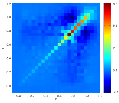
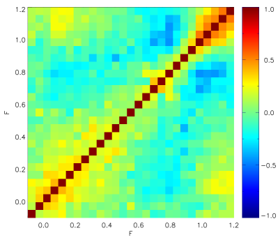
An advantage of our large sample size is that also able to directly estimate the error covariances, , via bootstrap resampling— an example is shown in Figure 7. In contrast to the Ly forest transmission PDF from high-resolution data which have significant off-diagonal covariances (Bolton et al. 2008), the error covariance from the BOSS transmission PDF is nearly diagonal with just some small correlations between neighboring bins, although we also see some anti-correlation between transmission bins at and .
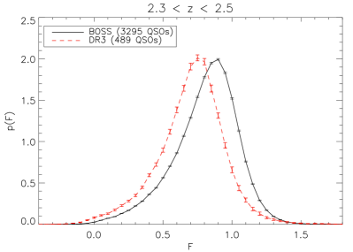
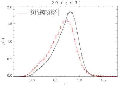
It is interesting to compare the transmission PDF from our data with that measured by Desjacques et al. (2007) from SDSS DR3. This comparison is shown in Figure 8, in which the transmission PDFs calculated from SDSS DR3 Ly forest spectra with (kindly provided by Dr. V. Desjacques) are shown for two redshift bins, juxtaposed with the BOSS transmission PDFs calculated from spectra with the same redshift and S/N cuts.
While there is some resemblance between the two PDFs, the most immediate difference is that the Desjacques et al. (2007) PDFs are shifted to lower transmission values, i.e., the mean transmission, , is considerably smaller than that from our BOSS data: and from their measurement, whereas the BOSS PDFs have and . This difference arises because the Desjacques et al. (2007) used a power-law continuum (albeit with corrections for the weak emission lines in the quasar continuum) extrapolated from in the quasar restframe; this does not take into account the power-law break that appears to occur in low-redshift quasar spectra at (Telfer et al. 2002; Suzuki 2006). Later in their paper, Desjacques et al. (2007) indeed conclude that this must be the case in order to be consistent with other measurements. Our continua, in contrast, have been constrained to match existing measurements of , for which there is good agreement between different authors at (e.g., Faucher-Giguère et al. 2008; Becker et al. 2013).
Another point of interest in Figure 8 is that the error bars of the BOSS sample are considerably smaller than those of the earlier measurement. This difference is largely due to the significantly larger sample size of BOSS. The proportion of pixels with appears to be smaller in the BOSS PDFs compared with the older data set, but this is because Desjacques et al. (2007) did not remove DLAs from their data.
We next describe the creation of mock Ly absorption spectra designed to match the properties of the BOSS data.
4. Modeling of the BOSS Transmission PDF
In this section, we will describe simulated Ly forest mock spectra designed, through a ‘forward-modelling’ process, to have the same characteristics as the BOSS spectra, for comparison with the observed transmission PDFs described in the previous section. For each BOSS spectrum which had contributed to our transmission PDFs in the previous section, we will take the Ly absorption from randomly selected simulation sightlines, then introduce the characteristics of the observed spectrum using auxiliary information returned by our pipeline.
Starting with simulated spectra from a set of detailed hydrodynamical IGM simulations, we carry out the following steps, which we will describe in turn in the subsequent subsections:
-
1.
Introduce LLS absorbers
-
2.
Smooth the spectrum to BOSS resolution
-
3.
Add metal absorption via an empirical method using lower-redshift SDSS/BOSS quasars
-
4.
Add pixel noise, based on the noise properties of the real BOSS spectrum using parameters estimated by our MCMC noise estimation technique
-
5.
Simulate continuum errors by refitting the noisy mock spectrum
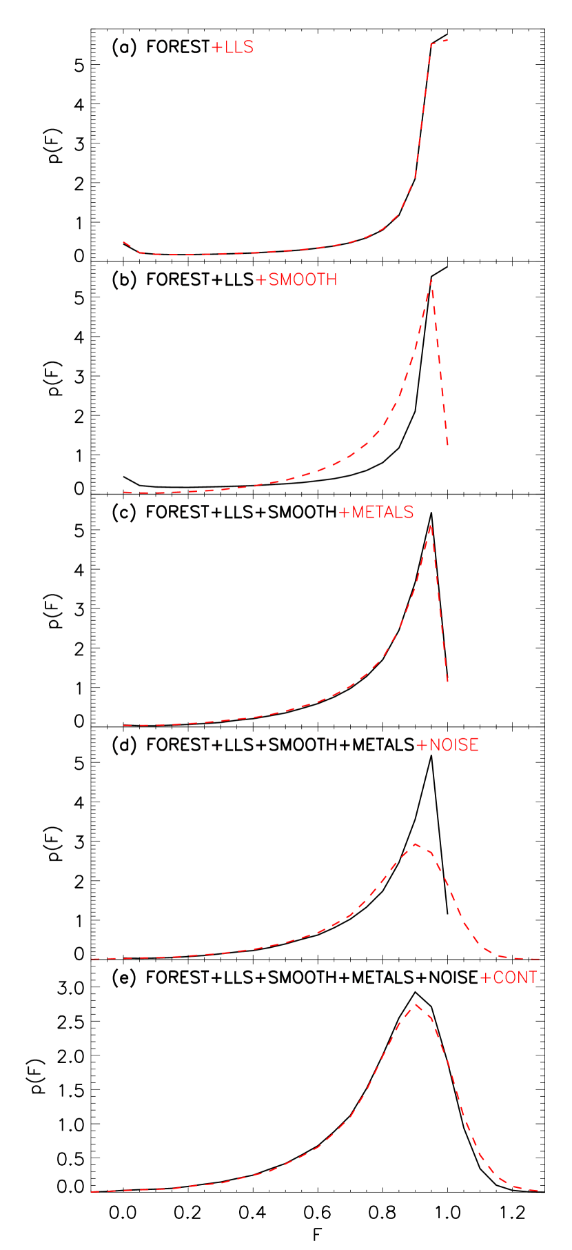
In the subsequent subsections, we will describe each step in detail. The effect of each step in on the observed transmission PDF is illlustrated in Figure 9.
4.1. Hydrodynamical Simulations
As the basis for our mock spectra, we use hydrodynamic simulations run with a modification of the publicly available GADGET-2 code. This code implements a simplified star formation criterion (Springel et al. 2005) that converts all gas particles that have an overdensity above 1000 and a temperature below K into star particles (see Viel et al. 2004). The simulations used are described in detail in Becker et al. (2011) and in Viel et al. (2013a).
The reference model that we use is a box of length 20 comoving Mpc with gas and cold DM particles (with a gravitational softening length of 1.3 kpc) in a flat CDM universe with cosmological parameters , , and , in agreement both with WMAP-9yr (Komatsu et al. 2011) and Planck data (Planck Collaboration et al. 2013). The initial condition power spectra are generated with CAMB (Lewis et al. 2000). For the boxes considered in this work, we have verified that the transmission PDF has converged in terms of box size and resolution.
We explore the impact of different thermal histories on the Ly forest by modifying the ultraviolet (UV) background photo-heating rates in the simulations as done in e.g., Bolton et al. (2008). A power-law temperature-density relation, , arises in the low density IGM () as a natural consequence of the interplay between photo-heating and adiabatic cooling (Hui et al. 1997; Gnedin & Hui 1998). The value of within a simulation can be modified by varying a density-dependent heating term (see, e.g., Bolton et al. 2008). We consider a range of values for the temperature at mean density, , and the power-law index of the temperature-density relation, , based on the observational measurements presented recently by Becker et al. (2011). These consist of a set of three different indices for the temperature-density relation, , that are kept roughly constant over the redshift range and three different temperatures at mean density, K, which evolve with redshift, yielding a total of nine different thermal histories. Between and there is some temperature evolution and the IGM becomes hotter at low redshift; at , the models have K. We refer to the intermediate temperature model as our ‘reference’ model, or T_REF, while the hot and cold models are referred to as T_HOT and T_COLD, respectively. The values of of our simulations at the various redshifts are summarized in Table 2.
| T_COLD | T_REF | T_HOT | |
|---|---|---|---|
| 2.3 | K | K | K |
| 2.6 | K | K | K |
| 3.0 | K | K | K |
Approximately 4000 core hours were required for each simulation run to reach . The physical properties of the Ly forest obtained from the TreePM/SPH code GADGET-2 are in agreement at the percent level with those inferred from the moving-mesh code AREPO (Bird et al. 2013) and with the Eulerian code ENZO (O’Shea et al. 2004).
For this study, the simulation outputs were saved at , from which we extract 5000 optical depth sightlines binned to 2048 pixels each. To convert these to transmission spectra, the optical depths were rescaled such that the skewers collectively yielded a desired mean-transmission, . For our fiducial models, we would like to use the mean-transmission values estimated byestimated by Becker et al. (2013), which we denote as for . However, their estimates assume certain corrections from optically-thick systems and metal absorption. We therefore add back in the corrections they made (see discussion in §3.2) to get their ‘raw’ measurement for that now includes all optically thick systems and metals, and then remove these contributions assuming our own LLS and metal absorption models (see below).
Later in the paper, we will argue that our PDF analysis in fact places independent constraints on .
4.2. Lyman-limit systems
In principle, all optically-thick Ly absorbers such as Lyman-limit systems (LLSs) and damped Ly absorbers (DLAs) should be discarded from Ly forest analyses, since they do not trace the underlying matter density field in the same way as the optically-thin forest (Equation 1), and require radiative transfer simulations to accurately capture their properties (e.g., McQuinn et al. 2011; Rahmati et al. 2013).
While DLAs are straightforward to identify through their saturated absorption and broad damping wings even in noisy BOSS data (see, e.g., Noterdaeme et al. 2012), the detection completeness of optically-thick systems through their Ly absorption drops rapidly at . Even in high-S/N, high-resolution spectra, optically thick systems can only be reliably detected through their Ly absorption at (“super-LLS”). Below these column densities, optically-thick systems can be identified either through their restframe Lyman-limit (albeit only one per spectrum) or using higher-order Lyman-series lines (e.g., Rudie et al. 2013). Neither of these approaches have been applied in previous Ly forest transmission PDF analyses (McDonald et al. 2000; Kim et al. 2007; Calura et al. 2012; Rollinde et al. 2013), so arguably all these analyses are contaminated by LLSs.
Instead of attempting to remove LLSs from our observed spectra, we instead incorporate them into our mock spectra through the following procedure. For each PDF bin, we evaluate the total redshift pathlength of the contributing BOSS spectra (and corresponding mocks) — this quantity is summarized in Table 1. This is multiplied by , the number of LLS per unit redshift, to give the total number of LLS expected within our sample. We used the published estimates of this quantity by Ribaudo et al. (2011)777Note that the value given in Table 6 of Ribaudo et al. (2011) is actually erroneous, and the correct normalization is in fact , consistent with the data in their paper, which is used in Equation 10. Dr. J. Ribaudo, in private communication, has concurred with this conclusion. which is valid over :
| (10) |
where and .
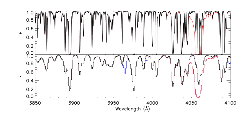
After estimating the total number of LLSs in our mock spectra, , we add them at random points within our set of simulated optical depth skewers. We also experimented with adding LLSs such that they are correlated with regions that already have high column density (e.g., Font-Ribera & Miralda-Escudé 2012), but we found little significant changes to the transmission PDF and therefore stick to the less computationally-intensive random LLSs.
For each model LLS, we then draw a column density using the published LLS column density distribution, , from Prochaska et al. (2010). This distribution is measured at , so we make the assumption that does not evolve with redshift between . For our column densities of interest, this distribution is represented by the broken power-laws:
| (11) |
For the normalizations and , we demand that
| (12) |
and require both power-laws to be continuous at . These constraints produce and . After drawing a random value for the column density of each LLS, we add the corresponding Voigt profile to the optical depth in the simulated skewer.
In addition to the LLS with column densities of that are defined to have , there is also a population of partial Lyman-limit systems (pLLSs) that are not well-captured in our hydrodynamical simulations since they have column densities () at which radiative transfer effects become significant (). However, the incidence rates and column-density distribution of pLLSs are ill-constrained since they are difficult to detect in normal LLS searches. We therefore account for the pLLS by extrapolating the low-end of the power-law distribution in Equation 11 down to , i.e.
| (13) |
This simple extrapolation does not take into account constraints from the mean-free path of ionizing photons (e.g., Prochaska et al. 2010) which predicts a steeper slope for the pLLS distribution, but we will explore this later in §5.2.
Comparing the integral of this extrapolated pLLS distribution with Equation 12 leads us to conclude that
| (14) |
and we proceed to randomly add pLLSs to our mock spectra in the same way as LLSs.
The other free parameter in our LLS model is their effective -parameter distribution. However, due to the observational difficulty in identifying LLSs the -parameter distribution of this distribution has, to our knowledge, never been quantified. Due to this lack of knowledge, it is common to simply adopt a single -value when attemping to model LLSs (e.g., Font-Ribera & Miralda-Escudé 2012; Becker et al. 2013). We therefore assume that all our pLLSs and LLSs have a -parameter of similar to DLAs (Prochaska & Wolfe 1997), an ‘effective’ value meant to capture the blending of multiple Ly components. However, the -parameter for this population of absorbers is a highly uncertain quantity and as we shall see, it will need to be modified to provide a satisfactory fit to the data although it will turn out to not strongly affect our conclusions regarding the IGM temperature-density relationship.
4.3. Spectral Resolution
The spectral resolution of SDSS/BOSS spectra is (Smee et al. 2013). The exact value varies significantly both as a function of wavelength, and across different fibers and plates depending on observing conditions (Figure 1).
For each spectrum, the BOSS pipeline provides an estimate of the wavelength dispersion at each pixel, , in units of the co-added wavelength grid size (). The spectral resolution at that pixel can then be obtained from the dispersion, through the following conversion: . Figure 1 shows the pixel dispersions from 236 randomly-selected BOSS quasar as a function of wavelength at the blue end of the spectrograph. Even at fixed wavelength, there is a considerable spread in the dispersion, e.g., ranging from at . The value of typically decreases with wavelength (i.e., the resolution increases).
In their analysis of the Ly forest 1D transmission power spectrum, Palanque-Delabrouille et al. (2013) made their own study of the BOSS spectral resolution by directly analysing the line profiles of the mercury and cadmium arc lamps used in the wavelength calibration. They found that the pipeline underestimates the spectral resolution as a function of fiber position (i.e. CCD row) and wavelength: the discrepancy is at blue wavelengths and near the CCD edges, but increases to as much as 10% at near the center of the blue CCD (c.f. Figure 4 in Palanque-Delabrouille et al. 2013). Our analysis is limited to , i.e. , where the discrepancy is under 4%. Nevertheless, we implement these corrections to the BOSS resolution estimate to ensure that we model the spectral resolution to an accuracy of .
For each BOSS Ly forest segment that contributes to the observed transmission PDFs discussed in § 3.3, we concatenate randomly-selected transmission skewers from the simulations described in the previous section. This is because the simulation box size of () is significantly shorter than the path length of our redshift bins (, or ). This ensures that each BOSS spectrum in our sample has a mock spectrum that is exactly matched in pathlength.
We then directly convolve the simulated skewers by a Gaussian kernel with a standard deviation that varies with wavelength, using the estimated resolution from the real spectrum, multiplied by the Palanque-Delabrouille et al. (2013) resolution corrections. The effect of smoothing on the transmission PDF is illustrated by the red-dashed curve in Figure 9b. Smoothing decreases the proportion of pixels with high-transmission () and with high-absorption (), and increases the number of pixels with intermediate transmission values.
4.4. Metal Contamination
Metal absorption along our observed Ly forest sightlines acts as a contaminant since their presence alters the observed statistics of the Ly forest. In high-resolution data, this contamination is usually treated by directly identifying and masking the metal absorbers, although in the presence of line blending it is unclear how thorough this approach can be.
With the lower S/N and moderate resolution of the BOSS data, direct metal identification and masking is not a viable approach. Furthermore, most of the weak metal absorbers seen in high-resolution spectra are not resolved in the BOSS data.
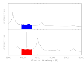
Rather than removing metals from the BOSS Ly forest spectra, we instead add metals as observed in lower-redshift quasar spectra. In other words, we add absorbers observed in the restframe region of lower-redshift quasars with , such that the observed wavelengths are matched to the Ly forest segment with average redshift . Figure 11 is a cartoon that illustrates this concept. This method makes no assumption about the nature of the metal absorption in the Ly forest, and includes all resolved metal absorption spanning the whole range of redshifts down to . The disadvantage of this method is that it does not include metals with intrinsic wavelengths , but the relative contribution of such metal species towards the transmission PDF should be small888Si III an obvious exception, but we will later account for this omission in our error bars (§5.3). since most of the metal contamination comes from low-redshift () C IV and Mg II.
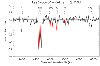
We use a metal catalogue generated by B. Lundgren et al. (in prep; see also Lundgren et al. 2009), which lists absorbers in SDSS (Schneider et al. 2010) and BOSS quasar spectra (Pâris et al. 2012) — the SDSS spectra were included in order to increase the number of quasars needed to introduce metals into the Ly forest mock spectra, which are not well sampled by the BOSS target selection (Ross et al. 2012). We emphasize that we work with the ‘raw’ absorber catalog, i.e. the individual absorption lines have not been identified in terms of metal species or redshift. For each quasar, the catalog provides a line list with the observed wavelength, equivalent width (EW, ), full-width at half-maximum (FWHM), and detection S/N, . To ensure a clean catalog, we use only absorbers in the catalog that were identified from quasar spectra with per angstrom redwards of Ly. The latter criterion ensures that even relatively weak lines (with ) are accounted for in our catalog. Figure 12 shows an example of the lower-redshift quasar spectra that we use for the metal modelling.
However, we want to add a smooth model of the metal-line absorption to add to our mock spectra, rather than adding in a noisy spectrum. We therefore use a simple model as follows: For each Ly forest segment we wish to model at redshift , we select an absorber line-list from a random quasar with . We next assume that all resolved metals in the SDSS/BOSS spectra are saturated and thus in the flat regime of the curve-of-growth. The equivalent width is then given by
| (15) |
where is the optical depth at line center, is the velocity width and is the speed of light. In the saturated regime, is mostly sensitive to changes in while being highly insensitive to changes in . We can thus adopt as a global constant and solve for , given the of each listed absorber in the selected ’sideband’ quasar. We have found that provides a good fit for most of the absorbers.
We then add the Gaussian profile into our simulated optical depth skewers:
| (16) |
centered at the same observed wavelength, , as the real absorber. The red curve in Figure 12 shows our model for the observed absorbers, using just the observed wavelength, , and equivalent width, , from the absorber catalog.
Our method for incorporating metals is somewhat crude since one should, in principle, first deconvolve the spectrograph resolution from the input absorbers, and then add the metal absorbers into our mock spectra prior to convolving with the BOSS spectral resolution. In contrast, we fit -parameters to the absorber catalog without spectral deconvolution, therefore these -parameters can be thought of as combinations of the true absorber width, and the spectral dispersion, , i.e. . While technically incorrect, this seems reasonable since the template quasar spectra and forest spectra that we are attempting to model both have approximately the same resolution, and in practical terms this ad hoc approach does seem to be able to reproduce the observed metals in the lower-redshift quasar spectra (Figure 12). The other possible criticism of our approach is that it does not incorporate weak metal absorbers, although we attempted to mitigate this by setting a very high S/N threshold on the template quasars for the metals. However, we have checked that such weak metals do not significantly change the forest PDF (and indeed metals in general do not seriously affect the PDF, c.f. Figure 9c).
We also tried adding metals with similar redshifts to — and correlated with — forest absorbers (e.g., absorption by Si II and Si III) measured in Pieri et al. (2010) and Pieri et al. (2014) using a method described in the appendix of Slosar et al. (2011). We found a negligible impact on the transmission PDF owing mainly to the fact that these correlated metals contribute only to the overall flux decrement, so we neglect this contribution in our subsequent analysis.
4.5. Pixel Noise
It is non-trivial to introduce the correct noise to a simulated Ly forest spectrum: given a noise estimate from the observed spectrum, one needs to first ensure that the mock spectrum has approximately the same flux normalization as the data. This is challenging, as the Ly forest transmission at any given pixel, which ranges from 0 to 1, will vary considerably between the simulated spectrum and the real data.
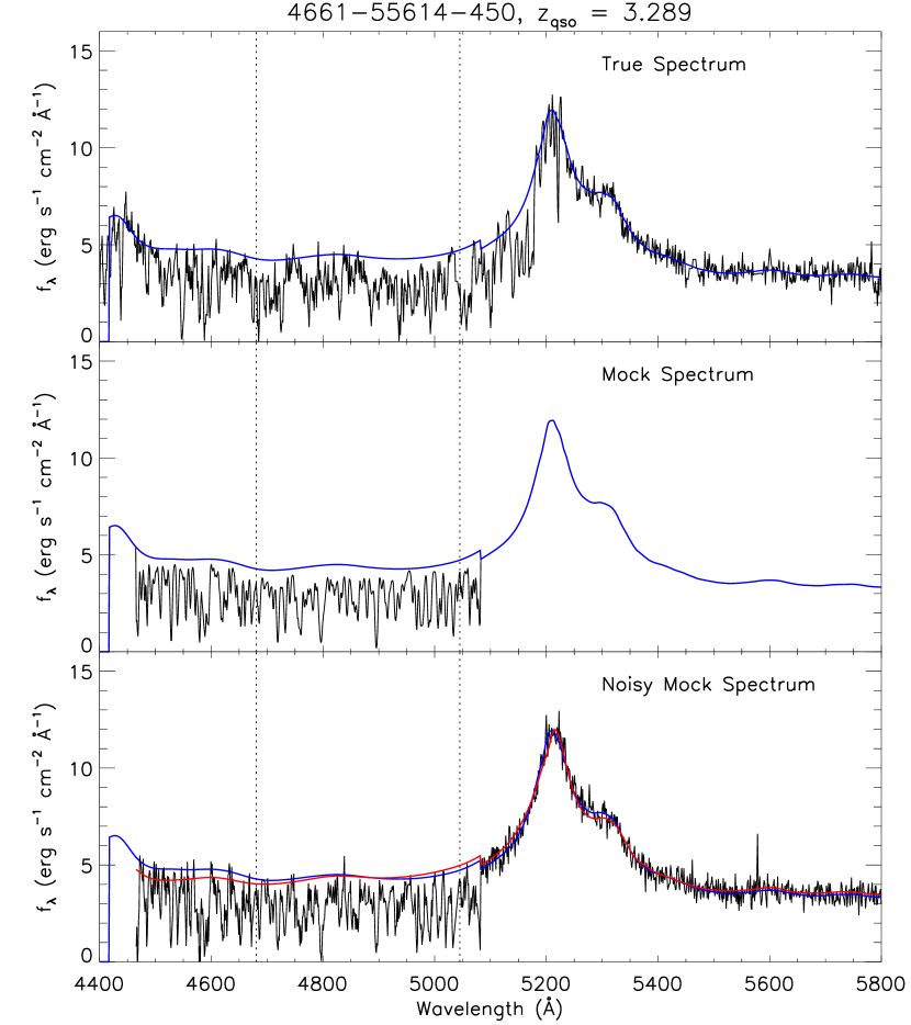
The simplest method of adding noise to a mock spectrum is simply to introduce Gaussian deviates using the pipeline noise estimate for each spectrum— this was essentially the method used by Desjacques et al. (2007) and the BOSS mocks described in Font-Ribera et al. (2012). However, with the MCMC co-addition procedure described in § 3.1, we are in a position to model the noise in a more robust and self-consistent fashion.
Recall that the MCMC procedure returns posterior probabilities for two quantities: the true underlying spectral flux density, , and the four free parameters , which parametrize the noise in each spectrum. This estimate of the from each quasar spectrum allows us to accurately model the pixel noise using Equation 5.
The MF-PCA method (§ 3.2) produces an estimate of the quasar continuum, , providing approximately the correct flux level at each point in the spectrum. We can now multiply with the simulated Ly forest transmission spectra, , which had already been smoothed to the same dispersion as its real counterpart (the estimated quasar continuum is already at approximately the correct smoothing, since it was fitted to the observed spectrum).
This procedure produces a noiseless mock spectrum with the correct flux normalization and smoothing. We can now generate noisy spectra corresponding to a given BOSS quasar, using our MCMC noise estimation described in Section 3.1. First, we substitute our mock spectrum as into Equation 5, and then combine the noise parameters (estimated through our MCMC procedure) as well as the calibration vectors and sky estimates . This lets us generate self-consistent noise vectors corresponding to each individual exposure that make up the mock quasar spectrum, . The noise vectors are then used to draw random Gaussian deviates that are added to the mock spectrum, on a per-pixel basis, to create the mock spectral flux density, . Finally, we combine these individual mock exposures into the optimal spectral flux density for the mock spectrum, through the expression (see Appendix):
| (17) |
where
| (18) |
Figure 9c illustrates the effect of adding pixel noise to the smoothed Ly forest transmission PDF. As expected, this scatters a significant fraction of pixels to , and also to to a smaller extent.
4.6. Continuum Errors
With the noisy mock spectrum in hand (see, e.g., bottom panel of Figure 13), we can self-consistently include the effect of continuum errors into our model transmission PDFs by simply carrying out our MF-PCA continuum-fitting procedure on the individual noisy mock spectra. Dividing out the mock spectra with the new continuum fits then incorporates an estimate of the continuum errors (estimated by Lee et al. 2012 to be at the RMS level) into the evaluated model transmission PDF. This estimated error includes uncertainties stemming from the estimation of the quasar continuum shape due to pixel noise, as well as the random variance in the mean Ly forest absorption in individual lines-of-sight.
Note that regardless of the overall mean-absorption in the mock spectra (i.e. inclusive of our models for metals, LLSs, and mean forest absorption — see § 5.4), we always use , the same input mean-transmission derived from Becker et al. (2013) (described in § 3.2) to fit the continua in both the data and mock spectra. While the overall absorption in our fiducial model is consistent with that from Becker et al. (2013), as we shall see later, the shape of the transmission PDF retains information on the true underlying mean-transmission even if fitted with a mean-flux regulated continuum with a wrong input .
The effect of continuum errors on the transmission PDF is shown in Figure 9e: like pixel noise, it degrades the peak of the PDF, but only near .
5. Model Refinement
In an ideal world, one would like to do a blind analysis by generating the transmission PDF model (§4) in isolation from the data, before ‘unblinding’ to compare with data — this would then in principle yield results free from psychological bias in the model building. However, as we shall see in §5.1, this does not give acceptable fits to the data so we have to instead modify our model to yield a better agreement, in particular our LLS model (§5.2) and assumed mean-transmission (§5.4).
5.1. Initial Comparison with T_REF Models
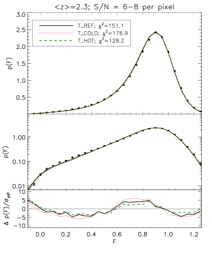
For each of our 9 hydrodynamical simulations (sampling 3 points each in and ), we determine the transmission PDF from the Ly forest mock spectra that include the effects described in the previous section, for the various redshift & S/N subsamples in which we had measured the PDF in BOSS (§3.3). In Figure 14, we show the transmission PDFs for all our redshift and S/N subsamples in BOSS, compared with the corresponding simulated transmission PDFs from the T_REF simulation with . Note that the error bars shown are the diagonal elements of the covariance matrix estimated through bootstrap resampling on the data.
At first glance, the model transmission PDFs seem to be a reasonably match for the data, especially considering we have carried out purely forward modelling without fitting for any parameters. However, when comparing the ‘pull’, , between the data and model (bottom panels of Figure 14), we see significant discrepancies in part due to the extremely small bootstrap error bars. Nevertheless, it is gratifying to see that the shape of the residuals are relatively consistent across the different S/N subsamples at fixed redshift and , since this indicates that our spectral noise model is robust.
We proceed to quantify the differences between the simulated transmission PDFs, , and observed transmission PDFs, , with the statistic:
| (19) |
where we use the bootstrap error covariance matrix, . Note that we also include a bootstrap error term that accounts for the sample variance in the model transmission PDFs, since our pipeline for generating mock spectra is too computationally expensive to include sufficiently large amounts of skewers to fully beat down the sample variance in the models999We aim for more mock spectra than in the corresponding data sample, but later when we have to compute large model grids we are limited to models with the same size as the data..
We limit our model comparison to the range , i.e. 27 transmission bins with bin width . This range covers pixels that have been scattered to ‘unphysical’ values of or due to pixel noise, as is expected from the low-S/N of our BOSS data, and also captures of the pixels within each of our data subsets. In particular, it is important to retain the bins with because the transmission bins are highly sensitive to (Lee 2012) and therefore we want to fully sample that region of the PDF even if it will require careful modeling of pixel noise and continuum errors.
There are two constraints on all our transmission PDFs: the normalization convention
| (20) |
and the imposition of the same mean transmission due to the mean-flux regulated continuum-fitting
| (21) |
such that all the mock spectra have the same absorption, . This is because the mock spectra have been continuum-fitted (§4.6) in exactly the same way as the BOSS spectra, which assumes the same mean Ly transmission inferred from the Becker et al. (2013) measurements (§3.2). The ‘true’ optically-thin mean-transmission, , imposed on the simulation skewers is in principle a different quantity from , since the latter includes contribution from metal contamination and optically-thick LLSs.
This leaves us with degrees of freedom (d.o.f.) in our comparison. The for all the models shown in Figure 14 are shown in the corresponding figure legends.
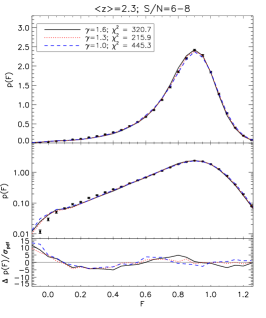
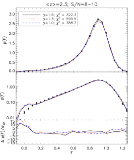
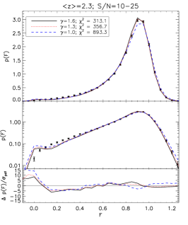
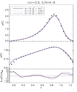
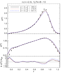
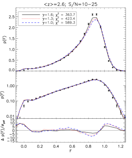
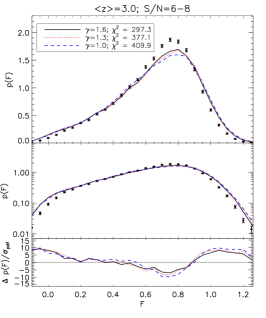
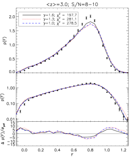
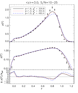
In this initial comparison, the values for the models in Figure 14 are clearly unacceptable: we find for 24 d.o.f. in all cases. However, it is interesting to note that the or models are preferred at all redshifts and S/N cuts. Note that the S/N= subsamples (middle column in Figure 14) tends to have a slightly better agreement between model and data compared to the other S/N cuts at the same redshift: this simply reflects the smaller quantity of data of the subsample (c.f. Table 1) and hence larger bootstrap errors.
A closer inspection of the residuals in Figure 14 indicate that there are two major sources of discrepancy between the models and data: firstly, at the low-transmission end, we underproduce pixels at while simultaneously over-producing pixels, especially at and . This seems to affect all models equally. Pieri et al. (2014) found that at BOSS resolution, pixels with come predominantly from saturated Ly absorption from LLS. We therefore investigate possible modifications to our LLS model in §5.2.
The other discrepancy in the model transmission PDFs manifests at the higher-transmission end in the and subsamples, where we see a sinusoidal shape in the residuals at that appears consistent across different S/N. This portion of the transmission PDF depends on both and, as we shall see, on the assumed mean-transmission , which we shall discuss in more detail in §5.4.
Finally, our transmission PDF model includes various uncertainties in the modelling of metals, LLSs, and continuum-fitting which have not yet been taken into account. In §5.3, we will estimate the contribution of these uncertainties, by means of a Monte-Carlo method, in our error covariances.
5.2. Modifying the LLS Column Density Distribution
With the moderate spectral resolution of BOSS, there are few individual pixels in the optically-thin Ly forest that reach transmission values of . Such low-transmission pixels are typically due to either the blending of multiple absorbers (see, e.g., Figure 2 in Pieri et al. 2014), or optically-thick systems (see Figure 10 in this paper).
As we have seen in Figure 14, at low-transmission values the discrepancy between data and model has a distinct shape, which is particularly clear at : the models underproduce pixels at while at the same time overproducing saturated pixels with .
To resolve this particular discrepancy would therefore require either drastically increasing the amount of clustering in the Ly forest, or modifying our assumptions on the LLSs in our mock spectra. The first possibility seems rather unlikely since the Ly forest power on relevant scales are well-constrained (Palanque-Delabrouille et al. 2013), and would in any case require new simulation suites to address — beyond the scope of this paper.
On the other hand, it is not altogether surprising that our fiducial column density distribution (§ 4.2) — which was measured at (Prochaska et al. 2010) — do not reproduce the BOSS data at . We therefore search for a LLS model that better describes the low-transmission end of the BOSS Ly forest. Looking at the PDFs in Figure 14, we see that our fiducial model over-produces pixels at , yet is deficient at slightly higher . This suggests that our model is over-producing super-LLS () that contribute large absorption troughs with , while not providing sufficient lower-column density absorbers that can individually reach minima of when smoothed to BOSS resolution. In other words, our fiducial model appears to have an excessively ‘top-heavy’ LLS column density distribution.
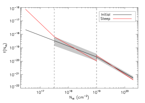
For a change, we will try a LLS column density distribution with a more ample bottom-end, using the steepest power-laws within the limits estimated by Prochaska et al. (2010):
| (22) |
We use the same as before, and obey the integral constraints from Prochaska et al. (2010) that demand that the ratios of between the two column-density regimes be fixed. This gives us and , although the new distribution is no longer continuous at . This new distribution is illustrated by the red power-laws in Figure 15.
Another change we have made is to the partial LLS model, which was possibly too conservative in the fiducial model. Instead of extrapolating from the LLS distribution, we now adopt the pLLS power-law slope of inferred from the total mean-free path to ionizing photons by Prochaska et al. (2010). This dramatically increases the incidence of pLLS in our spectra relative to LLS: we now have , where is the same value we used previously (Equation 10). This increase, while large, is not unreasonable in light of the large uncertainties in direct measurements on the H I column-density distribution from direct Ly line-profile fitting (e.g., Janknecht et al. 2006; Rudie et al. 2013). Note also that even this increased pLLS incidence only amounts to, on average, less than one pLLS per quasar ( per quasar at our redshifts).
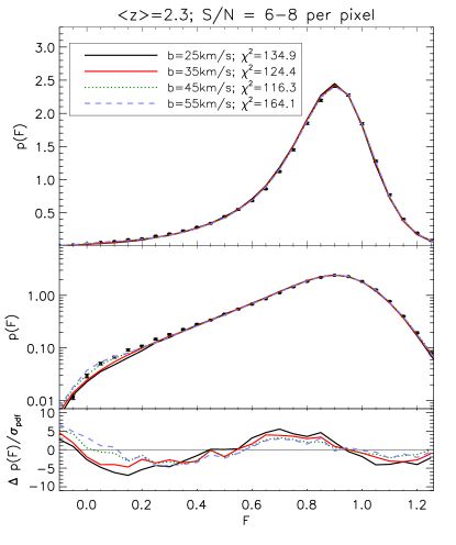
We found that while increasing the number of pLLS relieves the tension between data and model at , it does not resolve the excess at the fully absorbed pixels in the models. However, changing the -parameter of the LLS and pLLS from our original fiducial value of modifies the PDF in a way that improves the agreement. This is a reasonable step, since the effective -parameter is otherwise observationally ill-constrained for the LLS and pLLS populations. This is because LLSs are typically complexes of multiple systems separated in velocity space, and while there have been analyses of the -parameter in these individual components, the ‘effective’ -parameter for complete LLS systems has never been quantified to our knowledge.
We therefore search for the best-fit -parameter with respect to the T_REF, model at , focusing primarily on the agreement in the bins (Figure 16). Our choice of model for this purpose should not significantly affect our subsequent conclusions regarding the IGM temperature-density slope, since there is little sensitivity towards the latter in the relevant low-transmission bins (c.f. Figure 14). However, there will be some degeneracy between the LLS -parameter and (Figure 17) since changing the latter does somewhat change the low-transmission portion of the PDF — we will come back to this point in §7.
As shown in Figure 16, a value gives the best agreement with the data at . This yields for 24 d.o.f., which is dramatically improved over those quoted in Figure 14, but still not quite a good fit. In the subsequent results, we will adopt this steeper pLLS/LLS model and -parameter as the fiducial model in our analysis, and will correspondingly decrease the degrees of freedom in our analysis to account for the fitting of .
Note that while significantly improving the PDF fit, this new -parameter still does not give a perfect fit to the low-transmission () end. This is probably due to the simplified nature of our LLS model, which neglects the finite distribution of -parameters and internal velocity dispersion of individual components. These properties are currently not well-known, and it seems likely that an improved model would allow a better fit to the low-transmission end of the PDF.
5.3. Estimation of Systematic Uncertainties
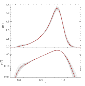
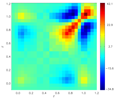
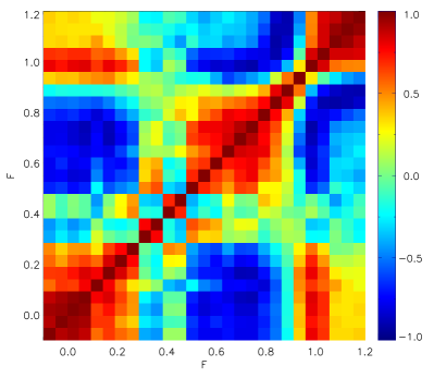
While we have estimated the sample variance of our BOSS transmission PDFs by bootstrap resampling on the spectra, there are significant uncertainties associated with each component of our transmission PDF model as described above, e.g., the LLS incidence rate and level of continuum error. These uncertainties can be incorporated into a systematics covariance matrix, that can then be added to the bootstrap covariance, , when computing the model likelihoods. This requires assuming that and are uncorrelated, and that the errors are Gaussian distributed.
We adopt a Monte Carlo approach to estimate by generating 200 model transmission PDFs that randomly vary the systematics. We then evaluate the covariance of the transmission PDFs, , relative to the fiducial model, at each transmission bin . This allows us to construct a covariance matrix with the elements
| (23) |
that encompasses the errors from the uncertainties in the LLS model, metal absorption, and continuum scatter. Note that estimation of systematic uncertainties is typically a subjective process, and for most of these contributions we can only make educated guesses as to their uncertainty.
Our Monte Carlo iterations sample the various components of our model as follows:
- LLS Incidence
- partial-LLS Slope
-
Our choice of slope for the distribution of partial LLS ( absorbers is from an indirect constraint with significant uncertainty (Prochaska et al. 2010). We therefore vary the pLLS slope around the fiducial by assuming a flat prior in this range, which primarily alters the portion of the PDF since pLLS typically do not saturate at BOSS resolution.
- LLS -parameters
-
Also in the previous section, we found that a global -parameter of gives the best agreement with the data, but this is an ad hoc approach with significant uncertainties. In our Monte Carlo Sampling we therefore adopt a conservative with a uniform prior. This primarily affects the PDF at as can be seen in Figure 16.
- Intervening Metals
-
Although we used an empirical method to model intervening metals (§ 4.4), we may have missed metals with rest wavelengths . Furthermore, we have a relatively small set () of ‘template’ quasars from which our metal model is derived, which may contribute some sampling variance. We therefore guess at an Gaussian error of for the metal incidence rate. This modulates the extent to which metals pulls the overall PDF towards lower -values (c.f. Figure 9c).
- Continuum Errors
-
The overall r.m.s. scatter in our continuum estimation also affect the flux PDF (Figure 9e). This can be varied in our model by rescaling the quantity , where is the ‘true’ continuum used to generate the mock spectrum, while is the model continuum which we subsequently fit (Figure 13). For each iteration in our Monte Carlo systematics estimation, we dilate or reduce by a Gaussian deviate assuming scatter. This primarily affects the high-transmission () end of the PDF.
For these Monte Carlo iterations, we used the identical thermal model (, T_REF) as well as fixed the same random number seeds used for the selection of simulation skewers and generation of noise vectors in our spectra, in order to ensure that the only variation between the different iterations are from the randomly-sampled systematics. Figure 18 shows 50 of these Monte Carlo iterations on the transmission PDF for the , S/N= subsample.
Figure 19 shows an example of the systematic contribution to the covariance matrix. The overall amplitude of the systematic contribution is considerably higher than that estimated from the bootstrap resampling (c.f. Figure 7), indicating that we are in the systematics-limited regime. We also see significant anti-correlations at almost the same level as the positive correlations, which are due mostly to correlations between transmission bins on either side of ‘pivot points’ as the transmission PDF varies from the systematics — these anti-correlations will somewhat counteract the increased size of the diagonal components. In the subsequent analysis, we will use an error covariance matrix, , in which the systematics covariance matrix estimated in this sub-section is added to the bootstrap covariance matrix (described in § 3.3) estimated from the BOSS transmission PDFs.
We have at this point yet to address one more parameter which can significantly change the shape of our model transmission PDFs, namely the Ly forest mean-transmission assumed in the mock spectra, . However, this is an important astrophysical parameter which we did not want to treat as a ‘systematic’, so the next sub-section will describe our treatment of .
5.4. Modifying the Mean-transmission
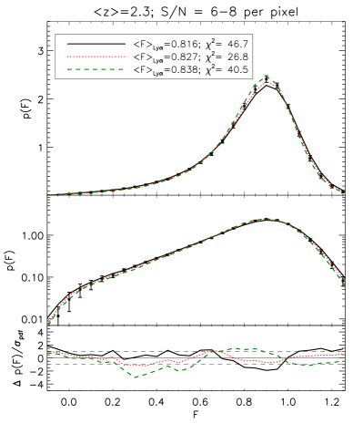
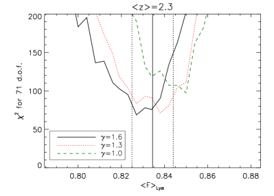
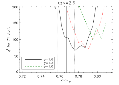
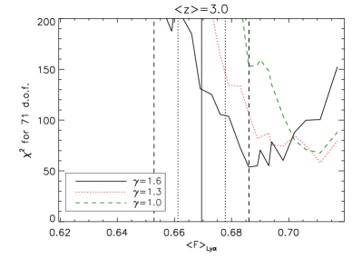
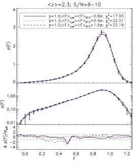
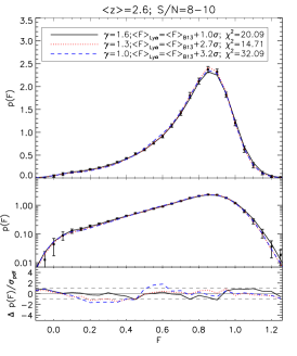
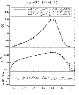
In the initial comparison of the model transmission PDFs shown in Figure 14, the models show a discrepancy with the data at higher transmission bins . Such differences can be alleviated by varying the mean-transmission of the pure Ly forest, , i.e. ignoring the contribution from metals and LLS. This quantity can be varied directly in the simulation skewers (Section 4.1). When we vary in the simulations, the quantity , which is used to normalize the continuum level of the mock quasar spectrum, is always kept fixed to as derived from Becker et al. (2013) (see Section 3.2). However, since we are applying the same to both the real and mock spectra, can be best thought of as a normalization that does not actually need to match . Once both the real and mock spectra have been normalized by , the transmission PDF retains information on the respective contributions from the Ly forest, metals and LLSs regardless of the assumed , because these contributions affect the shape of the PDF in different ways. In principle, it is possible to vary these all components to infer their relative contributions, but due to the crudeness of our metal and LLS models, we choose have only as a free parameter while keeping and fixed. The possible variation of these latter two components are instead incorporated into the systematic uncertainties determined in Section 5.3. The effect of varying is illustrated in Figure 20, where we plot the same IGM model with different underlying values of in the simulation skewers whilst keeping fixed the contribution from metals, LLSs etc.
We therefore explore a range of around the vicinity of that estimated by Becker et al. (2013), , and at each value of evaluate the summed over all the S/N subsamples for each and combination. In addition, we now adopt the updated LLS/pLLS model described in §5.2, while the evaluation now uses the full covariance matrix including both the bootstrap and systematics (§5.3) uncertainties to compare with the transmission PDFs measured from the BOSS data.
The models are compared with the BOSS data as we vary , and for each we compute the total chi-squared summed over all three S/N subsamples, where each subsample contributes d.o.f. (c.f. Equations 20 and 21) along with a further reduction of one d.o.f. since we have effectively fitted for the LLS -parameters in § 5.2, for a total of d.o.f. The result of this exercise is shown in Figure 21 which shows the values for the T_REF models with different — we only vary and not because the portions of the transmission PDF that change the most with do not vary as much with respect to changes in (c.f. Figure 17). Examples of the corresponding best-fit model PDFs in one S/N subsample are shown in Figure 22, where we see that varying can indeed change the shape of the portion of the transmission PDF sufficiently, improving the fits in those transmission ranges compared to the fiducial models (Figure 14).
In all our redshift bins, the best-fitting models seen in Figure 21 are with for 70 d.o.f.101010In this particular section, when we quote the for the best-fitting the d.o.f. is further reduced by 1 compared to the other summed over the S/N subsamples. at (for the combined data using all S/N bins), respectively implying probabilities of of getting larger values111111These values are very small for the degrees of freedom, suggesting that we may have overestimated the size of our systematic errors, but as we shall see this does not affect our ability to place constraints on and merely makes our conclusions rather conservative.. At the higher redshifts best-fitting mean-transmission for the case is pushed to significantly discrepant values with respect to the fiducial Becker et al. (2013) values (Figure 21).
The model also provide acceptable fits to the models, with for 70 d.o.f. () at , but at the two higher redshift bins this requires values that are increasingly discrepant compared to Becker et al. (2013) ( and respectively at ). The isothermal models are disfavored at the two lower redshift bins, with best-fit values of for 70 d.o.f. () at , whereas at , the error bars on the PDF are sufficiently large that acceptable fits are obtainable using , with for 70 d.o.f. (). However, this requires a discrepancy in with respect to Becker et al. (2013). In Figure 22, one sees that fitting for allows the models to be in good agreement with the data in the portion of the PDF, but gives rise to discrepancies in the range which limits the goodness-of-fit, and cannot easily be compensated by modifying the metals or LLS model.
From Figure 21, it is clear that as we move to higher redshifts, we require increasingly higher relative to the fiducial Becker et al. (2013) values in order to agree with the data: at , our best-fit mean-transmission for the model agrees with Becker et al. (2013), but at there is a significant deviation of with respect to the Becker et al. (2013) measurement. The same trend is true for the best-fit and models, but these require even greater discrepancies with respect to the fiducial .
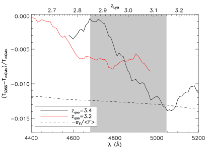
One possible explanation for this discrepancy is the effect on the Becker et al. (2013) measurement of -band selection bias in the SDSS quasars. This was first noted by Worseck & Prochaska (2011), who found that the color-color criteria used to select SDSS quasars preferentially selected quasars, specifically in the redshift range , that have intervening Lyman-breaks at . The SDSS quasars are thus more likely to have intervening LLS in their sightlines, yielding an additional contribution to the Ly absorption and hence causing Becker et al. (2013) to possibly underestimate when stacking the impacted quasars. Becker et al. (2013) mentioned this effect in their paper but argued that it was much smaller than their estimated errors by referencing theoretical IGM transmission curves estimated by Worseck & Prochaska (2011) (Figure 17 in the latter paper).
Dr. G. Worseck has kindly provided us with these transmission curves, , which were generated for both the average IGM absorption and that extracted from SDSS quasars affected by the color-color selection bias. In Figure 23 we plot the relative difference between the biased Ly transmission deduced from and quasars and the true mean IGM transmission, using the Worseck & Prochaska (2011) transmission curves. It is clear that at Ly absorption redshifts of , the excess LLS picked up from such quasars contribute an additional compared to the mean IGM decrement, a discrepancy that is of the same magnitude as the error bars in the Becker et al. (2013) measurement, indicated by the dashed line.
This could partially explain the higher required to make our models fit the data in Figure 21. Note that we expect this UV color selection bias to be much less significant in our BOSS data, since we have selected bright quasars in the top 5th percentile of the S/N distribution. Given that such quasars have high signal-to-noise ratio photometry, their colors separate much more cleanly from stellar contaminants. Furthermore, such bright quasars are much more likely to have been selected with multi-wavelength data (e.g., including near-IR and radio in addition to optical photometry see Ross et al. 2012). For both of these reasons, we expect our quasars to be much less susceptible to biases in color-selection related to the presence of an LLS. A careful accounting of this bias is beyond the scope of this paper, but from now on we will inflate by a factor of two the corresponding errors on at to account for this possible bias in the mean transmission measurements (dashed vertical lines in bottom panel of Figure 21).
Another possibility that could explain a bias in the measured by Becker et al. (2013) is their assumption that the metal contamination of the Ly forest does not evolve with redshift. While there are few clear constraints on the aggregate metal contamination within the forest, assuming that the metals actually decrease with increasing redshfit (e.g., in the case of C IV, Cooksey et al. 2013), then the assumption of an unevolving metal contribution calibrated at would lead to an underestimate of at higher redshifts, which could explain the trend we seem to be seeing.
It is clear from the previous discussion that there is some degeneracy between and in our transmission PDFs. However, we are primarily interested in , while the has been extensively measured over the years allowing strong priors to be placed. In the next section, we will therefore marginalize over in order to obtain our final results.
6. Results
Due to the uncertainties in described in the previous sub-section, for a better comparison between transmission PDFs, , from models with different we will marginalize the model likelihoods, , over the Ly forest mean-transmission, :
| (24) |
where is the prior on (for clarity in these equations, is used as a shorthand for ). We assume a Gaussian prior:
| (25) |
where and are the optically-thin Ly forest mean-transmission and associated errors, respectively, estimated from Becker et al. (2013). Note that for , we have decided to dilate the error bars by a factor of to account for the suspected quasar selection bias discussed in the previous section.
For each model, we generate transmission PDFs with different (similar to Figure 21) and evaluate the combined summed over different S/N. We interpolate the over to obtain a finer grid, which then allows us to numerically integrate Equation 24 using five-point Newton-Coates quadrature.
At this stage, we also analyze models with different IGM temperatures at mean-density, . Hitherto, we have been working only with the central T_REF model (K) , but we now also compare models from the T_HOT and T_COLD simulations, that have K and K, respectively. Each of these temperature models also sample temperature-density relationships of for a model grid of parameters at each redshift.
| T_COLD | T_REF | T_HOT | |
| (K) | (K) | (K) | |
| 1.6 | 87.7 | 72.9 | 79.5 |
| 1.3 | 103.4 | 76.0 | 71.8 |
| 1.0 | 174.2 | 105.5 | 88.4 |
| T_COLD | T_REF | T_HOT | |
| (K) | (K) | (K) | |
| 1.6 | 88.8 | 72.0 | 71.4 |
| 1.3 | 118.0 | 82.6 | 91.8 |
| 1.0 | 203.3 | 127.3 | 111.1 |
| T_COLD | T_REF | T_HOT | |
| (K) | (K) | (K) | |
| 1.6 | 61.7 | 65.1 | 62.5 |
| 1.3 | 77.6 | 72.7 | 63.8 |
| 1.0 | 119.5 | 77.7 | 85.8 |
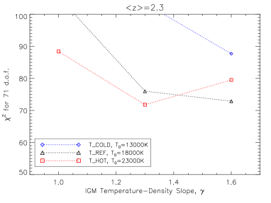
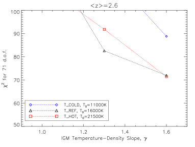
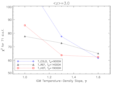
The marginalized values for all the models are tabulated in Table 3, and plotted as a function of in Figure 24. In general, the T_REF models with provide the best agreements with the data at all redshifts with for 69 d.o.f.. The T_HOT models (with higher IGM temperatures at mean density) provide fits of comparable quality, and indeed at the T_HOT model with gives essentially the same goodness-of-fit as the T_REF model. The cooler T_COLD models are less favored by the data, and at give unreasonable fits to the data with for 69 d.o.f. (), but at other redshifts they are acceptable fits to the data. In other words, the transmission PDF does not show a strong sensitivity for , which we shall show later is due to degeneracy with our LLS model in the low-transmission end of the transmission PDF.
The more important question to address is the possibility of isothermal or inverted temperature-density relationships () as suggested by some studies on the transmission PDF of high-resolution, high-S/N echelle quasar spectra (e.g., Bolton et al. 2008; Viel et al. 2009; Calura et al. 2012). It is clear from Table 3 and Figure 24 that for all models the isothermal, models disagree strongly with the BOSS data. The closest match for an isothermal IGM is the T_REF model at , which yields for 69 d.o.f., or a probability of 21% of obtaining the data from this model. However, relative to the model at which gives the minimum at that redshift, we find for the isothermal model, i.e. a discrepancy from the best-fit model. The isothermal model is also strongly disfavored at the other redshifts, where we find at or . Since the shape of the transmission PDF varies continuously as a function of (see, e.g., Bolton et al. 2008; Lee 2012), these results imply that inverted () IGM temperature-density slopes are even more strongly ruled out.
7. Discussion
In this paper, we have studied the Ly forest transmission probability distribution function (PDF) from 3373 BOSS DR9 quasar spectra. Although this is a relatively small subsample selected to be in the top 95th percentile in terms of S/N, they provide 2 orders-of-magnitude larger Ly forest path length than high-resolution, high-S/N data sets previously used for this purpose, providing unprecedented statistical power for transmission PDF analysis.
In order to ensure accurate characterization and allow subsequent modelling of the spectral noise, we have introduced a novel, probabilistic method of combining the multiple exposures that comprise each BOSS observation, using the raw sky and calibration data. This method significantly improves the accuracy of the noise estimation, and additionally allows us to generate mock spectra with noise properties tailored to each individual BOSS spectrum, but self-consistently for different Ly forest realizations. We believe that our noise modeling — which yields noise estimates accurate to across the relevant wavelength range — is the most careful treatment of spectral noise in multi-object fiber spectra to-date, and we invite readers with similarly stringent requirements in understanding the BOSS spectral noise to contact the authors. In the future, the spectral extraction algorithm described by Bolton & Schlegel (2010) may solve some of the issues which affected us, but this has yet to be implemented.
For the continuum estimation, we used the mean-flux regulated/principal component analysis (MF-PCA) method introduced in Lee (2012). This method, which reduces the uncertainty in the continuum estimation to , fits for a continuum such that the resulting Ly forest has a mean-transmission matched to external constraints, for which we use the precise measurements by Becker et al. (2013). While MF-PCA does require external constraints for , we argue that so long as both the real quasars and mock spectra are continuum-fitted in exactly the same way, the shape of the transmission PDF retains independent information on the Ly forest mean-transmission.
To compare with the data, we used the detailed hydrodynamical simulations of Viel et al. (2013a), that explore a range of IGM temperature-density slopes () and temperatures at mean density (K). We processed the simulated spectra to take account the characteristics of the individual BOSS spectra in our sample, such as spectral resolution, pixel noise, and continuum fitting errors. We also incorporate the effects of astrophysical ‘nuisance’ parameters such as Lyman-limit systems (LLSs) and metal contamination. The LLSs are modeled by adding absorbers into our mock spectra, based on published measurements of the observed incidence (Ribaudo et al. 2011) and H I column density distribution (Prochaska et al. 2010). Meanwhile, contamination from lower-redshift metals are modeled in an empirical fashion by inserting absorbers observed in lower-redshift SDSS/BOSS quasars into the same observed wavelengths of our mock spectra.
Our initial models did not provide satisfactory agreement with the transmission PDF measured from the BOSS spectra, with discrepancies at both the high-transmission and low-transmission bins. However, the differences between data and models were consistent across the different S/N subsamples, indicating that our noise modelling is robust. To resolve the discrepancies at the low-transmission end of the PDF, we explored various modifications to our LLS model. Firstly, we steepened the column-density distribution slope of partial LLS ( systems) to a value suggested from the mean-free path of ionizing photons (Prochaska et al. 2010). This change relieved the tension between model and data in the bins, but implies increasing the number of pLLS by nearly an order of magnitude, but this is not unreasonable given the current uncertainties on this population (Janknecht et al. 2006; Prochaska et al. 2010). We believe that the necessity of a pLLS distribution with to fit the BOSS Ly transmission PDF supports the claims of Prochaska et al. (2010) regarding the column-density distribution of this population.
However, after adding pLLSs a major discrepancy remained in the saturated bins, which we addressed by adjusting the effective -parameter assumed in all the optically-thick systems in our model. We found that an effective value of gave the best-fit to our model121212Note that we have quoted an effective -parameter, which must not be confused with the from individual kinematical components, which is often quoted by workers carrying out Voigt profile analysis of high-resolution spectra..
At the high-transmission () end of the model transmission PDFs, we found that modifying the Ly forest mean-transmission in the simulations, , allowed much better agreement with the BOSS data. At , the that gave the best-fitting model PDFs were within of the Becker et al. (2013) measurements, but at we required a value that was larger. We argue that this discrepancy could be due to a color-color selection bias in the SDSS quasars used by Becker et al. (2013), which preferentially selected sightlines with intervening LLS, giving rise to additional Ly absorption (and thus lower ) at a level comparable to the errors estimated by Becker et al. (2013). Our BOSS spectra, on the other hand, should be comparatively unaffected on account of being the brightest quasars in the survey, hence they they separate more cleanly from the stellar locus in color-space, and were more likely to have been selected with additional criteria (radio, near-IR, variability etc) beyond color-color information (Ross et al. 2012).
To deal with these uncertainties, we decided to marginalize over the mean-transmission in our analysis. At , the preferred model is for a hot IGM with (K) along with (), although the intermediate-temperature model (K) with is nearly as good a fit with . The preferred models at are for at temperatures at mean-density of K (, respectively. We find that the isothermal () temperature-density relationship is strongly disfavored at all redshifts regardless of , with discrepancies of compared to the best-fit models.


One might be skeptical of the results given the various assumptions we had to make in modelling astrophysical nuisance parameters. To test the robustness of our results to systematics, we generated 20 iterations of model transmission PDFs sampling all nine of our models (i.e. 180 PDFs in total) in the , S/N=8-10 bin, where each iteration has a random realization of the systematics (LLS, metals, continuum errors etc) drawn in the same way as our Monte-Carlo estimate of systematic uncertainty (§5.3). We then asked how many times each or model gave the lowest when compared with the data. For this test we only evaluated the at the fiducial without marginalization.
The results of this test is shown in Figure 25. In the top panel, the T_REF and T_HOT models are favored of the time but the T_COLD has of being favored depending on the (random) choice of systematics. In other words, there is significant degeneracy between our systematics model and . We suspect this is driven largely by the choice of the LLS -parameter, which changes the shape of the transmission PDF in a similar way to (compare Figure 16 with Figure 17). In contrast, the bottom panel of Figure 25 shows that whatever systematics we choose, is always favored indicating a robust constraint.
There is however some degeneracy between and the Ly forest mean transmission, . While we marginalize over the latter quantity, the choice of prior can, in principle, affect the results. However, at , the chi-squared minimum of the PDF model as a function of is for 71 d.o.f. (Figure 21), which has a probability of . In other words, even if we fine-tuned in an attempt to force the isothermal model as the best-fit model at these redshifts, it would still be an unacceptable fit, and the model would still be preferred over it. This is less clear-cut at , where the error bars are large enough to permit a reasonable minimum chi-squared of for 71 d.o.f. using the model, but this requires a value of , which is discrepant from the value reported by Becker et al. (2013). While this measurement is dependent on corrections for metals and LLS absorption (and indeed we argue that they have neglected a subtle bias related to SDSS quasar selection), they have attempted to incorporate these uncertainties into their errors and we have no particular reason to believe that they have underestimated this by a factor of . A quick survey of the available measurements on the forest mean-transmission from the past decade yield (Kim et al. 2007; Faucher-Giguère et al. 2008; Dall’Aglio et al. 2008), albeit with larger errors. The use of any of these measurements as priors for our analysis would therefore disfavor an IGM with , (which requires ), unless all the available literature in the field have significantly underestimated the mean-transmission.
There are several cosmological and astrophysical effects that we did not model, that could in principle affect our conclusions on . Since the Ly forest transmission PDF essentially measures the contrast between high-absorption and low-absorption regions of the IGM, this can be degenerate with the underlying amplitude of matter fluctuations which is specified by a combination of and , the matter fluctuation variance on scales and the slope of the amplitude power spectrum, respectively. While these parameters are increasingly well-constrained (e.g., Planck Collaboration et al. 2013), there is still some uncertainty regarding the level of the fluctuations on the sub-Mpc scales relevant to the Ly forest which could be degenerate with our measurement. Bolton et al. (2008) explored this degeneracy between and in the context of transmission PDF measurements from high-resolution spectra, and found that the PDF is less sensitive to plausible changes in compared to , e.g. modifying by , affected the shape of the PDF less than a modification of (Figure 2 in their paper). This degeneracy is in fact further weakened when an MCMC analysis of the full parameter space is considered, as shown by the likelihood contours in Viel et al. (2009).
The astrophysical effects that could be degenerate with include galactic winds and inhomogeneities in the background UV ionizing field. The injection of gas into the IGM by strong galaxy outflows could in principle modify Ly forest statistics at fixed ; this was studied using hydrodynamical simulations by Viel et al. (2013b), who concluded that the effect on the PDF is small compared to the uncertainties in high-resolution PDF measurements. Our BOSS measurement has roughly the same errors as those from high-resolution spectra once systematic uncertainties are taken into account, therefore it seems unlikely that galactic winds could significantly bias our conclusions on . Meanwhile, fluctuations in the UV ionizing background, , that are correlated with the overall density field could also be degenerate with the temperature-density relationship (c.f. Equation 1). This effect was studied by McDonald et al. (2005a) in simulations using an extreme model that considered only UV background contributions from highly-biased AGN, which maximizes the inhomogeneities. They concluded that while these UV fluctuations affected forest transmission statistics at , the effect was small at , the redshift range of our measurements.
Various observational and systematic effects could also, in principle, affect our constraints on . For example, our modeling of the BOSS spectral resolution assumes a Gaussian smoothing kernel which might affect our constraints if this were untrue. However, in their analysis of the 1D forest transmission power spectrum, Palanque-Delabrouille et al. (2013) examined the BOSS smoothing kernel and did not find significant deviations from Gaussianity. There are also possible systematics caused by our simplified modeling of LLS and metal contamination in the data, for example in our assumption of a single -parameter for all LLSs and our neglect of very weak metal absorbers. However, we believe that the test performed in Figure 25 samples larger differences in the transmission PDF than those caused by our model simplifications, e.g. it seems unlikely that going from a single LLS -parameter to a finite -distribution could cause to greater differences in the flux PDF than varying the single -parameter by as was done in Figure 25. As for continuum-estimation, we carry out the exact same continuum-fitting procedure on the mock spectra as on the real quasar spectra, which leads no overall bias since in both cases the resulting forest transmission field is forced to have the same overall transmission, . The only uncertainty then relates to the distribution of , i.e. the per-pixel error of the estimated continuum, , relative to the true continuum, . In reality the shape of this distribution could be different between the data and mocks, whereas within our mocks framework we could only explore overall rescalings of the distribution width. Again, we find it unlikely that differences in the transmission PDF caused by the true shape of the distribution could be so large as to be comparable to the effect caused by varying the width of the continuum error distribution, that we have examined.
While we do not think that the effects described in the previous few paragraphs qualitatively affect our conclusion that the BOSS data is inconsistent with isothermal or inverted IGM temperature-density relationships (), when taken in aggregate these systematic uncertainties do weaken our formal limits against and need to explicitly considered in future analyses.
7.1. Astrophysical Implications
How does this compare with other results on the thermal state of the IGM? McDonald et al. (2001) analyzed the transmission PDF from 8 high-resolution, high S/N spectra and compared with now-obsolete hydrodynamical simulations. They found the data to be consistent with a temperature-density relationship (TDR) with the expected values of (Hui & Gnedin 1997). More recently, Bolton et al. (2008) and Viel et al. (2009) carried out analyses of the transmission PDF measured from a larger sample (18 spectra) of Ly forest sightlines measured by Kim et al. (2007) and found evidence for an inverted TDR (). Viel et al. (2009) found that at , the temperature-density relation was highly inverted (), and remained so as low as although at the lower redshifts the data was marginally consistent with an isothermal IGM. They suggested the difference between their results and those of McDonald et al. (2001) was due to the now-obsolescent cosmological parameters and less-detailed treatment of intervening metals in the earlier study. However, Lee (2012) then pointed out that there is a sensitivity of the measured values of from the transmission PDF on continuum-fitting. Since continuum-fitting of high-resolution data generally involves manually placing the continuum at Ly forest transmission peaks which do not necessarily reach the true continuum, it is conceivable that continuum biases combined with underestimated jacknife errors bars (e.g., Rollinde et al. 2013) could have led Bolton et al. (2008) and Viel et al. (2009) to erroneously deduce an inverted temperature-density relation (see Bolton et al. 2014 for a detailed discussion on this point). In our analysis we have fitted our continua using an automated process that is free from the same continuum-fitting bias, although it does require an assumption on the underlying Ly forest transmission which we have marginalized over in our analysis.
Most recent measurements of the transmission PDF from high-resolution data have continued to favor an isothermal or inverted — Calura et al. (2012) analyzed the transmission PDF from a sample of quasars and also found an isothermal TDR at , although combining with the Kim et al. (2007) data drove the estimated to inverted values at . However, Rollinde et al. (2013) carried out a re-analysis of the transmission PDF from various high-resolution echelle data sets, which included significant overlap with the Kim et al. (2007) data. They argue that previous analyses have underestimated the error on the transmission PDF, and found the observed transmission PDF to be consistent with simulations that have over — this discrepancy is probably also driven by a different continuum-estimation from the Kim et al. (2007) measurement.
The use of other statistics on high-resolution spectra have however tended to disfavor an isothermal or inverted TDR. Rudie et al. (2012) analyzed the lower-end of the - cutoff from individual Ly forest absorbers measured in a set of 15 very high-S/N quasar echelle spectra, and estimated at . Bolton et al. (2014) compared the Rudie et al. (2012) measurements to hydrodynamical simulations and corroborated their determination of the TDR slope.
Garzilli et al. (2012) analyzed the Kim et al. (2007) sample and found that while the transmission PDF supports an isothermal or inverted TDR, a wavelet analysis favors . Note, however, that the - cutoff and the transmission PDF are sensitive to different density ranges, with the PDF probing gas densities predominantly below the mean (e.g., Bolton et al. 2014).
Our result of at are thus in rough agreement with measurements that do not involve the transmission PDF from high-resolution Ly forest spectra (with the exception of Rollinde et al. 2013). Our value of at is somewhat unexpected because one expects a flattening of the TDR close to the He II reionization epoch at (Furlanetto & Oh 2008; McQuinn et al. 2009; but see Gleser et al. 2005; Meiksin & Tittley 2012), but is not strongly disfavored ()
Taken at face value, the TDR during He II reionization can be made steeper by a density-independent reionization and/or a lower heating rate in the IGM (Furlanetto & Oh 2008), which could be reconciled with an extended He II event (Shull et al. 2010; Worseck et al. 2011).
Our constraints on appear to be in conflict with the prediction of the theories of Broderick et al. (2012) and Chang et al. (2012), who elucidated a relativistic pair-beam channel for plasma-instability heating of the IGM from TeV gamma-rays produced by a population of luminous blazars. This mechanism provides a uniform volumetric heating rate, which would cause an inverted TDR in the IGM (Puchwein et al. 2012) since voids would experience a higher specific heating rate compared with heating by He II reionization alone. This picture has been challenged by the recent study of Sironi & Giannios (2014), who dispute the amount of heating this mechanism could provide, since they found that the momentum dispersion of such relativistic pair beams allows of the beam energies to be deposited into the IGM.
However, in this paper we have assumed relatively simple TDRs in which the bulk of the IGM in the density range follows a relatively tight power-law. We have therefore not studied more complicated relationships, e.g., with a spread of temperatures at fixed density (e.g., Meiksin & Tittley 2012; Compostella et al. 2013) that might be caused by He II reionization or other phenomena. It is therefore possible that such complicated TDRs could result in Ly forest transmission PDFs that mimic the power-law; this is something that needs to be examined in more detail in future work.
7.2. Future Prospects
Looking forward, the subsequent BOSS data releases will significantly enlarge our sample size, e.g., DR10 (Ahn et al. 2014) is nearly double the size of the DR9 sample used in this paper, while the final BOSS sample (DR12) should be three times as large as DR9. In particular, the newer data sets should be sufficiently large for us to analyze the transmission PDF and constrain during the epoch of He II reionization at . This would be a valuable measurement, since high-resolution spectra are particularly affected by continuum-fitting biases at these redshifts (Faucher-Giguère et al. 2008; Lee 2012).
The analysis of the optically-thin Ly forest transmission PDF from these expanded data sets will have vanishingly small sample errors, and the errors will be dominated by systematic and astrophysical uncertainties. At the high-transmission end, our uncertainties are dominated by the scatter of the continuum-fitting, which is dominated by the question of whether our quasar PCA templates, derived from low-luminosity low-redshift quasars (Suzuki et al. 2005), or high-luminosity SDSS quasars (Pâris et al. 2011), respectively, are an accurate representation of the BOSS quasars. This uncertainty should be eliminated in the near-future by PCA templates derived self-consistently from the BOSS data (Nao Suzuki et al. 2014, in prep). The modelling of metal contamination could also be improved in the near future by advances in our understanding of how metals are distributed in the IGM (e.g., Zhu et al. 2014), although metals are a comparatively minor contribution to the uncertainty in our transmission PDF.
We also aim to improve on the rather ad hoc data analysis in this paper, in which we accounted for some uncertainties in our modelling by incorporating them into our error covariances (e.g., LLSs, metals, continuum errors), while was marginalized over a fixed grid. In future analyses, it would make sense to carry out a full Markov Chain Monte Carlo treatment of all these parameters which would rigorously account for all the uncertainties and allow straightforward marginalization over nuisance parameters.
Since this paper was initially focused on modelling the BOSS spectra, for the model comparison we used only simulations sampling a very coarse grid in and parameter space, and were unable to take account for uncertainties in other cosmological (, etc) and astrophysical (e.g., Jeans’ scale, Rorai et al. 2013; or galactic winds, Viel et al. 2013b) parameters in our analysis. However, methods already exist to interpolate Ly forest statistics from hydrodynamical simulations given a set of IGM and cosmological parameters (e.g., Viel & Haehnelt 2006; Borde et al. 2014; Rorai et al. 2013). In the near future we expect to do joint analyses using other Ly forest statistics in conjunction with the transmission PDF, such as new measurements of the small-scale () 1D transmission power spectrum (Walther et al. 2014, in prep.), moderate-scale () transmission power spectrum in both 1D (e.g., Palanque-Delabrouille et al. 2013) and 3D (from ultra-dense Ly forest surveys using high-redshift star-forming galaxies, Lee et al. 2014a, b), the phase angle probability distribution function determined from close quasar pair sightlines (Rorai et al. 2013), and others. Such efforts would require a fine grid sampling the full set of cosmological and IGM thermal parameters in order to ensure that the interpolation errors are small compared to the uncertainties in the data (see e.g., Rorai et al. 2013). Efforts are underway to utilize massively-parallel adaptive-mesh refinement codes (Almgren et al. 2013) to generate such parameter grids to study the IGM (Lukić et al. 2014) However, one of the findings of this paper is the importance of correct modelling of LLS, in particular partial LLS (), in accounting for the shape of the observed Ly transmission PDF. Since our hydrodynamical simulations did not include radiative transfer and cannot accurately capture optically thick systems, we had to add these in an ad hoc manner based on observational constraints which are currently rather imprecise. In the near future, we would want to use hydrodynamical simulations with radiative transfer (even if only in post-processing, e.g., Altay et al. 2011; McQuinn et al. 2011; Altay et al. 2013; Rahmati et al. 2013) to self-consistently model the optically-thick absorbers in the IGM. With the unprecedented statistical power of the full BOSS Ly forest sample, this could provide the opportunity to place unique constraints on the column-density distribution function of partial LLS.
8. Summary/Conclusions
In this paper, we analyzed the probability distribution function (PDF) of the Ly forest transmitted flux using 3393 BOSS quasar spectra (with ) from Data Release 9 of the SDSS-III survey.
To rectify the inaccurate noise estimates in the standard pipeline, we first carried a custom co-addition of the individual exposures of each spectrum, using a probabilistic procedure that also separates out the signal and CCD contributions, allowing us to later create mock spectra with realistic noise properties. We then estimated the intrinsic quasar continuum using a mean-flux regulated technique that reduces the scatter in the estimated continua by forcing the resultant Ly forest mean transmission to match the precise estimates of Becker et al. (2013), although we had to make minor corrections on the latter to account for our different assumptions on optically-thick systems in the data. This now allows us to measure the transmission PDF in the data, which we do so at (with bin widths of ), and split into S/N subsamples of S/N = [6-8, 8-10, 10-25] at each redshift bin.
The second part of the paper describe finding a transmission PDF model which describes the data, based on detailed hydrodynamical simulations of the optically-thin Ly forest that sample different IGM temperature-density relationship slopes, , and temperatures at mean-density, (where ). Using these simulations we generate mock spectra based on the real spectra. These take into account the following instrumental and astrophysical effects:
- Lyman-Limit Systems
-
These are randomly added into our mock spectra based on published incidence rates (Ribaudo et al. 2011) and column-density distributions (Prochaska et al. 2010), including a large population of partial LLS () with a power-law distribution of roughly . We assumed an effective for the velocity width of these absorbers.
- Metal Contamination
-
We measure metal absorption rom the restframe region of lower-redshift quasars at the same observed wavelength, then add these directly into our mock spectra.
- Spectral Resolution and Noise
-
Each mock spectrum is smoothed by the dispersion vector of the corresponding real spectrum (determined by the BOSS pipeline), and we apply corrections which bring the spectral resolution modeling to within accuracy. We then introduce pixel noise based on the noise parameters estimated by our probabilistic co-addition procedure on the real data, which also achieves percent level accuracy on modeling the noise.
- Continuum Errors
-
Since we generate a full mock Ly forest spectrum including the simulated quasar continuum (based on the continua fitted to the actual data), we can apply our continuum-estimation procedure on each mock to fit a new continuum. The difference between the new continuum and the underlying simulated quasar continuum yields an estimate of the continuum error.
We then compare the model transmission PDFs with the data, using an error covariance that includes both bootstrap errors and systematic uncertainties in the model components described above. At we find a discrepancy in the assumed Ly forest mean-transmission, , between our data and that derived from Becker et al. (2013), which we argue is likely caused by a selection bias in the SDSS quasars used by the latter. We therefore marginalize out these uncertainties in to obtain our final results.
The models with an IGM temperature-density slope of give the best-fit to the data at all our redshift bins (). Models with an isothermal or inverted temperature-density relationship () are disfavored at the at , respectively. Due to a degeneracy with our LLS model, we are unable to put robust constraints on but we have checked that our conclusions on are robust to such systematics as can be considered within our model framework. There are other possible systematics we did not consider that could in principle affect our measurement, such as cosmological parameters (, ) and astrophysical effects (galactic winds, inhomogeneous UV ionizing background), but we argue that these are unlikely to qualitatively affect our conclusions.
References
- Abazajian et al. (2005) Abazajian, K., Adelman-McCarthy, J. K., Agüeros, M. A., et al. 2005, AJ, 129, 1755
- Abazajian et al. (2009) Abazajian, K. N., Adelman-McCarthy, J. K., Agüeros, M. A., et al. 2009, ApJS, 182, 543
- Ahn et al. (2012) Ahn, C. P., Alexandroff, R., Allende Prieto, C., et al. 2012, ApJS, 203, 21
- Ahn et al. (2014) —. 2014, ApJS, 211, 17
- Almgren et al. (2013) Almgren, A. S., Bell, J. B., Lijewski, M. J., Lukić, Z., & Van Andel, E. 2013, ApJ, 765, 39
- Altay et al. (2013) Altay, G., Theuns, T., Schaye, J., Booth, C. M., & Dalla Vecchia, C. 2013, MNRAS, 436, 2689
- Altay et al. (2011) Altay, G., Theuns, T., Schaye, J., Crighton, N. H. M., & Dalla Vecchia, C. 2011, ApJ, 737, L37
- Anderson et al. (2014) Anderson, L., Aubourg, É., Bailey, S., et al. 2014, MNRAS, 441, 24
- Becker et al. (2011) Becker, G. D., Bolton, J. S., Haehnelt, M. G., & Sargent, W. L. W. 2011, MNRAS, 410, 1096
- Becker et al. (2013) Becker, G. D., Hewett, P. C., Worseck, G., & Prochaska, J. X. 2013, MNRAS, 430, 2067
- Bernardi et al. (2003) Bernardi, M., Sheth, R. K., SubbaRao, M., et al. 2003, AJ, 125, 32
- Bird et al. (2013) Bird, S., Vogelsberger, M., Sijacki, D., et al. 2013, MNRAS, 429, 3341
- Bolton & Schlegel (2010) Bolton, A. S., & Schlegel, D. J. 2010, PASP, 122, 248
- Bolton et al. (2012) Bolton, A. S., Schlegel, D. J., Aubourg, É., et al. 2012, AJ, 144, 144
- Bolton et al. (2014) Bolton, J. S., Becker, G. D., Haehnelt, M. G., & Viel, M. 2014, MNRAS, 438, 2499
- Bolton et al. (2009) Bolton, J. S., Oh, S. P., & Furlanetto, S. R. 2009, MNRAS, 395, 736
- Bolton et al. (2008) Bolton, J. S., Viel, M., Kim, T., Haehnelt, M. G., & Carswell, R. F. 2008, MNRAS, 386, 1131
- Borde et al. (2014) Borde, A., Palanque-Delabrouille, N., Rossi, G., et al. 2014, ArXiv e-prints, arXiv:1401.6472
- Bovy et al. (2011) Bovy, J., Hennawi, J. F., Hogg, D. W., et al. 2011, ApJ, 729, 141
- Broderick et al. (2012) Broderick, A. E., Chang, P., & Pfrommer, C. 2012, ApJ, 752, 22
- Busca et al. (2013) Busca, N. G., Delubac, T., Rich, J., et al. 2013, A&A, 552, A96
- Calura et al. (2012) Calura, F., Tescari, E., D’Odorico, V., et al. 2012, MNRAS, 422, 3019
- Cen et al. (1994) Cen, R., Miralda-Escudé, J., Ostriker, J. P., & Rauch, M. 1994, ApJ, 437, L9
- Chang et al. (2012) Chang, P., Broderick, A. E., & Pfrommer, C. 2012, ApJ, 752, 23
- Compostella et al. (2013) Compostella, M., Cantalupo, S., & Porciani, C. 2013, MNRAS, 435, 3169
- Cooksey et al. (2013) Cooksey, K. L., Kao, M. M., Simcoe, R. A., O’Meara, J. M., & Prochaska, J. X. 2013, ApJ, 763, 37
- Croft et al. (1998) Croft, R. A. C., Weinberg, D. H., Katz, N., & Hernquist, L. 1998, ApJ, 495, 44
- Dall’Aglio et al. (2008) Dall’Aglio, A., Wisotzki, L., & Worseck, G. 2008, A&A, 491, 465
- Davé et al. (1999) Davé, R., Hernquist, L., Katz, N., & Weinberg, D. H. 1999, ApJ, 511, 521
- Dawson et al. (2013) Dawson, K. S., Schlegel, D. J., Ahn, C. P., et al. 2013, AJ, 145, 10
- Desjacques et al. (2007) Desjacques, V., Nusser, A., & Sheth, R. K. 2007, MNRAS, 374, 206
- Draine (2011) Draine, B. T. 2011, Physics of the Interstellar and Intergalactic Medium (Princeton University Press)
- Eisenstein et al. (2011) Eisenstein, D. J., Weinberg, D. H., Agol, E., et al. 2011, AJ, 142, 72
- Faucher-Giguère et al. (2008) Faucher-Giguère, C., Prochaska, J. X., Lidz, A., Hernquist, L., & Zaldarriaga, M. 2008, ApJ, 681, 831
- Font-Ribera et al. (2012) Font-Ribera, A., McDonald, P., & Miralda-Escudé, J. 2012, JCAP, 1, 1
- Font-Ribera & Miralda-Escudé (2012) Font-Ribera, A., & Miralda-Escudé, J. 2012, JCAP, 7, 28
- Furlanetto & Oh (2008) Furlanetto, S. R., & Oh, S. P. 2008, ApJ, 682, 14
- Garzilli et al. (2012) Garzilli, A., Bolton, J. S., Kim, T.-S., Leach, S., & Viel, M. 2012, MNRAS, 424, 1723
- Gleser et al. (2005) Gleser, L., Nusser, A., Benson, A. J., Ohno, H., & Sugiyama, N. 2005, MNRAS, 361, 1399
- Gnedin & Hui (1998) Gnedin, N. Y., & Hui, L. 1998, MNRAS, 296, 44
- Gunn & Peterson (1965) Gunn, J. E., & Peterson, B. A. 1965, ApJ, 142, 1633
- Gunn et al. (2006) Gunn, J. E., Siegmund, W. A., Mannery, E. J., et al. 2006, AJ, 131, 2332
- Horne (1986) Horne, K. 1986, PASP, 98, 609
- Hui & Gnedin (1997) Hui, L., & Gnedin, N. Y. 1997, MNRAS, 292, 27
- Hui et al. (1997) Hui, L., Gnedin, N. Y., & Zhang, Y. 1997, ApJ, 486, 599
- Hui & Haiman (2003) Hui, L., & Haiman, Z. 2003, ApJ, 596, 9
- Janknecht et al. (2006) Janknecht, E., Reimers, D., Lopez, S., & Tytler, D. 2006, A&A, 458, 427
- Jenkins & Ostriker (1991) Jenkins, E. B., & Ostriker, J. P. 1991, ApJ, 376, 33
- Kim et al. (2007) Kim, T., Bolton, J. S., Viel, M., Haehnelt, M. G., & Carswell, R. F. 2007, MNRAS, 382, 1657
- Komatsu et al. (2011) Komatsu, E., Smith, K. M., Dunkley, J., et al. 2011, ApJS, 192, 18
- Lee (2012) Lee, K.-G. 2012, ApJ, 753, 136
- Lee et al. (2014a) Lee, K.-G., Hennawi, J. F., White, M., Croft, R. A. C., & Ozbek, M. 2014a, ApJ, 788, 49
- Lee & Spergel (2011) Lee, K.-G., & Spergel, D. N. 2011, ApJ, 734, 21
- Lee et al. (2012) Lee, K.-G., Suzuki, N., & Spergel, D. N. 2012, AJ, 143, 51
- Lee et al. (2013) Lee, K.-G., Bailey, S., Bartsch, L. E., et al. 2013, AJ, 145, 69
- Lee et al. (2014b) Lee, K.-G., Hennawi, J. F., Stark, C., et al. 2014b, ApJ, 795, L12
- Lewis et al. (2000) Lewis, A., Challinor, A., & Lasenby, A. 2000, ApJ, 538, 473
- Lidz et al. (2010) Lidz, A., Faucher-Giguère, C.-A., Dall’Aglio, A., et al. 2010, ApJ, 718, 199
- Lukić et al. (2014) Lukić, Z., Stark, C., Nugent, P., et al. 2014, ArXiv e-prints, arXiv:1406.6361
- Lundgren et al. (2009) Lundgren, B. F., Brunner, R. J., York, D. G., et al. 2009, ApJ, 698, 819
- Lynds (1971) Lynds, R. 1971, ApJ, 164, L73
- McDonald & Eisenstein (2007) McDonald, P., & Eisenstein, D. J. 2007, Phys. Rev. D, 76, 063009
- McDonald et al. (2001) McDonald, P., Miralda-Escudé, J., Rauch, M., et al. 2001, ApJ, 562, 52
- McDonald et al. (2000) —. 2000, ApJ, 543, 1
- McDonald et al. (2005a) McDonald, P., Seljak, U., Cen, R., Bode, P., & Ostriker, J. P. 2005a, MNRAS, 360, 1471
- McDonald et al. (2005b) McDonald, P., Seljak, U., Cen, R., et al. 2005b, ApJ, 635, 761
- McDonald et al. (2006) McDonald, P., Seljak, U., Burles, S., et al. 2006, ApJS, 163, 80
- McQuinn et al. (2009) McQuinn, M., Lidz, A., Zaldarriaga, M., et al. 2009, ApJ, 694, 842
- McQuinn et al. (2011) McQuinn, M., Oh, S. P., & Faucher-Giguère, C.-A. 2011, ApJ, 743, 82
- McQuinn & White (2011) McQuinn, M., & White, M. 2011, MNRAS, 415, 2257
- Meiksin & Tittley (2012) Meiksin, A., & Tittley, E. R. 2012, MNRAS, 423, 7
- Meiksin (2009) Meiksin, A. A. 2009, Reviews of Modern Physics, 81, 1405
- Miralda-Escudé et al. (1996) Miralda-Escudé, J., Cen, R., Ostriker, J. P., & Rauch, M. 1996, ApJ, 471, 582
- Miralda-Escudé & Rees (1994) Miralda-Escudé, J., & Rees, M. J. 1994, MNRAS, 266, 343
- Noterdaeme et al. (2012) Noterdaeme, P., Petitjean, P., Carithers, W. C., et al. 2012, A&A, 547, L1
- O’Shea et al. (2004) O’Shea, B. W., Bryan, G., Bordner, J., et al. 2004, ArXiv Astrophysics e-prints, arXiv:astro-ph/0403044
- Palanque-Delabrouille et al. (2013) Palanque-Delabrouille, N., Yèche, C., Borde, A., et al. 2013, A&A, 559, A85
- Pâris et al. (2011) Pâris, I., Petitjean, P., Rollinde, E., et al. 2011, A&A, 530, A50
- Pâris et al. (2012) Pâris, I., Petitjean, P., Aubourg, É., et al. 2012, A&A, 548, A66
- Penton et al. (2000) Penton, S. V., Shull, J. M., & Stocke, J. T. 2000, ApJ, 544, 150
- Petitjean et al. (1993) Petitjean, P., Webb, J. K., Rauch, M., Carswell, R. F., & Lanzetta, K. 1993, MNRAS, 262, 499
- Pieri et al. (2010) Pieri, M. M., Frank, S., Weinberg, D. H., Mathur, S., & York, D. G. 2010, ApJ, 724, L69
- Pieri et al. (2014) Pieri, M. M., Mortonson, M. J., Frank, S., et al. 2014, MNRAS, 441, 1718
- Planck Collaboration et al. (2013) Planck Collaboration, Ade, P. A. R., Aghanim, N., et al. 2013, ArXiv e-prints, arXiv:1303.5076
- Prochaska et al. (2005) Prochaska, J. X., Herbert-Fort, S., & Wolfe, A. M. 2005, ApJ, 635, 123
- Prochaska et al. (2010) Prochaska, J. X., O’Meara, J. M., & Worseck, G. 2010, ApJ, 718, 392
- Prochaska & Wolfe (1997) Prochaska, J. X., & Wolfe, A. M. 1997, ApJ, 487, 73
- Puchwein et al. (2012) Puchwein, E., Pfrommer, C., Springel, V., Broderick, A. E., & Chang, P. 2012, MNRAS, 423, 149
- Rahmati et al. (2013) Rahmati, A., Pawlik, A. H., Raic̆evic̀, M., & Schaye, J. 2013, MNRAS, 430, 2427
- Rauch (1998) Rauch, M. 1998, ARA&A, 36, 267
- Rauch et al. (1992) Rauch, M., Carswell, R. F., Chaffee, F. H., et al. 1992, ApJ, 390, 387
- Ribaudo et al. (2011) Ribaudo, J., Lehner, N., & Howk, J. C. 2011, ApJ, 736, 42
- Ricotti et al. (2000) Ricotti, M., Gnedin, N. Y., & Shull, J. M. 2000, ApJ, 534, 41
- Rollinde et al. (2013) Rollinde, E., Theuns, T., Schaye, J., Pâris, I., & Petitjean, P. 2013, MNRAS, 428, 540
- Rorai et al. (2013) Rorai, A., Hennawi, J. F., & White, M. 2013, ApJ, 775, 81
- Ross et al. (2012) Ross, N. P., Myers, A. D., Sheldon, E. S., et al. 2012, ApJS, 199, 3
- Rudie et al. (2012) Rudie, G. C., Steidel, C. C., & Pettini, M. 2012, ApJ, 757, L30
- Rudie et al. (2013) Rudie, G. C., Steidel, C. C., Shapley, A. E., & Pettini, M. 2013, ApJ, 769, 146
- Schaye et al. (2003) Schaye, J., Aguirre, A., Kim, T.-S., et al. 2003, ApJ, 596, 768
- Schaye et al. (1999) Schaye, J., Theuns, T., Leonard, A., & Efstathiou, G. 1999, MNRAS, 310, 57
- Schaye et al. (2000) Schaye, J., Theuns, T., Rauch, M., Efstathiou, G., & Sargent, W. L. W. 2000, MNRAS, 318, 817
- Schmidt (1965) Schmidt, M. 1965, ApJ, 141, 1295
- Schneider et al. (2010) Schneider, D. P., Richards, G. T., Hall, P. B., et al. 2010, AJ, 139, 2360
- Seljak et al. (2005) Seljak, U., Makarov, A., McDonald, P., et al. 2005, Phys. Rev. D, 71, 103515
- Shull et al. (2010) Shull, J. M., France, K., Danforth, C. W., Smith, B., & Tumlinson, J. 2010, ApJ, 722, 1312
- Sironi & Giannios (2014) Sironi, L., & Giannios, D. 2014, ApJ, 787, 49
- Slosar et al. (2011) Slosar, A., Font-Ribera, A., Pieri, M. M., et al. 2011, JCAP, 9, 1
- Slosar et al. (2013) Slosar, A., Iršič, V., Kirkby, D., et al. 2013, JCAP, 4, 26
- Smee et al. (2013) Smee, S. A., Gunn, J. E., Uomoto, A., et al. 2013, AJ, 146, 32
- Springel et al. (2005) Springel, V., Di Matteo, T., & Hernquist, L. 2005, MNRAS, 361, 776
- Stoughton et al. (2002) Stoughton, C., Lupton, R. H., Bernardi, M., et al. 2002, AJ, 123, 485
- Suzuki (2006) Suzuki, N. 2006, ApJS, 163, 110
- Suzuki et al. (2005) Suzuki, N., Tytler, D., Kirkman, D., O’Meara, J. M., & Lubin, D. 2005, ApJ, 618, 592
- Telfer et al. (2002) Telfer, R. C., Zheng, W., Kriss, G. A., & Davidsen, A. F. 2002, ApJ, 565, 773
- Theuns et al. (1998) Theuns, T., Leonard, A., Efstathiou, G., Pearce, F. R., & Thomas, P. A. 1998, MNRAS, 301, 478
- Theuns et al. (2002) Theuns, T., Schaye, J., Zaroubi, S., et al. 2002, ApJ, 567, L103
- Tytler et al. (2004) Tytler, D., Kirkman, D., O’Meara, J. M., et al. 2004, ApJ, 617, 1
- Vanden Berk et al. (2001) Vanden Berk, D. E., Richards, G. T., Bauer, A., et al. 2001, AJ, 122, 549
- Viel et al. (2013a) Viel, M., Becker, G. D., Bolton, J. S., & Haehnelt, M. G. 2013a, Phys. Rev. D, 88, 043502
- Viel et al. (2009) Viel, M., Bolton, J. S., & Haehnelt, M. G. 2009, MNRAS, 399, L39
- Viel & Haehnelt (2006) Viel, M., & Haehnelt, M. G. 2006, MNRAS, 365, 231
- Viel et al. (2004) Viel, M., Haehnelt, M. G., & Springel, V. 2004, MNRAS, 354, 684
- Viel et al. (2013b) Viel, M., Schaye, J., & Booth, C. M. 2013b, MNRAS, 429, 1734
- Worseck & Prochaska (2011) Worseck, G., & Prochaska, J. X. 2011, ApJ, 728, 23
- Worseck et al. (2011) Worseck, G., Prochaska, J. X., McQuinn, M., et al. 2011, ApJ, 733, L24
- York et al. (2000) York, D. G., Adelman, J., Anderson, Jr., J. E., et al. 2000, AJ, 120, 1579
- Zhu et al. (2014) Zhu, G., Ménard, B., Bizyaev, D., et al. 2014, MNRAS, 439, 3139
In this Appendix, we describe our probabilistic procedure for combining the multiple BOSS exposures of each spectrum131313Defined as unique combinations of plate number, fiber number and MJD of observation. while simultaneously estimating the noise variance in terms of a parametrized model. We assume the noise in each pixel can be described by
| (1) |
where
| (2) |
The true object flux and are noise parameters which we will determine given the individual exposure spectra , sky flux estimates , and calibrations vectors (which convert between detector counts and photons). is the effective read noise which we fixed to ; this can be thought of as an effective number of pixels times the true read noise of the CCD squared, which we multiplied by the spectrograph dispersion to approximately account for the change in spot-size as a function of wavelength. Equation 2 parametrizes wavelength-dependent biases in the calibration vector.
We search for the model that best describes the multiple exposure spectra , where our model parameters are from Eq. (1) and is the true flux of the object. In what follows, we will outline a method for determining the posterior distribution using a Markov Chain Monte Carlo (MCMC) method. From this distribution, we can obtain both an accurate model for the noise via Eq. (1), and our final combined spectrum. The estimates for can also be used to self-consistently generate pixel noise in mock Ly forest spectra.
The probability of the data given the model, or the likelihood, can be written
| (3) | |||||
Note that individual exposure data are on the native wavelength grid of each CCD exposure, whereas the BOSS pipeline interpolates and then combines these individual spectra into a final co-added spectrum, defined on a wavelength grid with uniform spacing. Furthermore, flexure and other variations in the spectrograph wavelength solution will result in small (typically sub-pixel) shifts between the individual exposure wavelength grids. In Eq. (3) our model must be computable at every wavelength of the individual exposures. We are free to choose the wavelengths at which is represented, but this choice is a subtle issue for several reasons. First, note that we want to avoid interpolating the data, , onto the model wavelength grid, as this would correlate the data pixels, and require that we track covariances in the likelihood in Eq. (3), making it significantly more complicated and challenging to evaluate. Similarly, it is undesirable to interpolate our model , as this would introduce correlations in the model parameters, making it much more difficult to sample them with our MCMC. Finally, note that also represents our final co-added spectrum, so we might consider opting for a a uniform wavelength grid, similar to what is done by the BOSS pipeline. Our approach is to simply determine the model flux at each wavelength of the individual exposures . Shifts among the individual exposure wavelength grids result in a more finely sampled model grid. For the reasons explained above, we use nearest grid point (NGP) interpolation, so that the are evaluated on the grid (and vice versa) by assigning the value from the single nearest pixel.
In our MCMC iterations, we use the standard Metropolis-Hastings criterion to sample the parameters , with trials drawn from a uniform prior. For the , we exploit an analogy with Gibbs sampling, which dramatically simplifies MCMC for likelihood functions with a multivariate Gaussian form. Gibbs sampling exploits the fact that given a multivariate distribution, it is much simpler to sample from conditional distributions than to integrate over a joint distribution. To be more specific, the likelihood in Eq. (3) is proportional to the joint probability distribution of the noise parameters and , but it is also proportional to the conditional probability distribution of the at fixed . With fixed the probability of is then
| (4) |
which is very nearly a multivariate Gaussian distributions for with a diagonal covariance matrix. The equation above slightly deviates from a Gaussian because the depend on via Eq. (1). In what follows, we ignore this small deviation, and assume that the conditional PDF of the (at fixed ) is Gaussian.
Given that Eq. 4 is a multivariate Gaussian with diagonal covariance, the Gibbs sampling of the becomes trivial. Since, Eq. (4) can be factored into a product of individual Gaussians, we need not follow the standard Gibbs sampling algorithm, whereby each parameter is updated sequentially holding the others fixed. Instead we need only hold fixed (since the likelihood is not Gaussian in these parameters), and we can sample all of the simultaneously. This simplification, which dramatically speeds up the algorithm, is possible because the conditional distribution for can be factored into a product of Gaussians for each pixel , thus the conditional distribution at any wavelength is completely independent of all the others.
Completing the square in Eq. (4) we can then write
| (5) |
where
| (6) |
The expressions above for and simply represent the optimally combined flux estimator and the resulting variance. Thus one can think of our MCMC algorithm as performing an optimal combination of the individual exposure spectra , whereby the noise is simultaneously determined via an iterative procedure.
Thus the basic steps of our algorithm can be summarized as follows:
-
•
Initialize, by creating a model grid from all unique wavelengths in the individual exposures, and use NGP interpolation to assign a to this grid for each exposures.
-
•
Choose a starting guess for noise parameters . For the starting use from Eq. (6), but with the model replaced by the noise delivered by the pipeline
-
•
Begin the MCMC loop:
-
1.
Use the current values of and to compute the variance for each exposure via Eq. (1).
-
2.
Compute and from Eq. 6.
-
3.
Take a Gibbs step for each wavelength of simultaneously, where is a vector of unit variance Gaussian deviates.
-
4.
Use NGP to interpolate the model onto each individual exposure wavelength grid.
-
5.
Compute the likelihood according to Eq. (3)
-
6.
Take trial steps in the according to , where is a stepsize and is a Gaussian deviate between zero and one, drawn for each individual noise parameter .
-
7.
Compute the likelihood at
-
8.
Apply the Metropolis-Hastings criteria to the likelihood difference. If it is satisfied then accept the values of as part of the Markov chain. If not, then use the previous values. Note that the are always accepted, because they are Gibbs sampled.
-
1.
-
•
Use only the second half of the chain for the posterior distributions, as the first half is the burn in phase.
Our MCMC algorithm directly determines the posterior distribution , which provides all the information we need to construct mock spectra using Eq. (1) as described in §4.5.
The distribution of , on the other hand, contains everything we need to know about the combined spectrum. Namely, we can define
| (7) |
as the combined spectrum, and
| (8) |
as its variance. If the formal noise returned by BOSS pipeline were actually the true noise in the data, then our in Eq. (8) would be equivalent to the optimally combined noise and our variance the optimal variance, i.e. according to Eq. (6). In practice, the BOSS pipeline does not return the true noise and so our is optimal whereas the pipeline flux is sub-optimal, and our is an empirical estimate of the actual noise in the data.