Long-range spatial correlations of particle displacements and the emergence of elasticity

Abstract

We examine correlations of transverse particle displacements and their relationship to the shear modulus of a glass and the viscosity of a fluid. To this end we use computer simulations to calculate a correlation function of the displacements, $S_{4}(q;t)$, which is similar to functions used to study heterogeneous dynamics in glass-forming fluids. We show that in the glass the shear modulus can be obtained from the long-time, small-q limit of $S_{4}(q;t)$. By using scaling arguments, we argue that a four-point correlation length $\xi_{4}(t)$ grows linearly in time in a glass and grows as $\sqrt{t}$ at long times in a fluid, and we verify these results by analyzing $S_{4}(q;t)$ obtained from simulations. For a viscoelastic fluid, the simulation results suggest that the crossover to the long-time $\sqrt{t}$ growth of $\xi_{4}(t)$ occurs at a characteristic decay time of the shear stress autocorrelation function. Using this observation, we show that the amplitude of the long-time $\sqrt{t}$ growth is proportional to $\sqrt{\eta}$ where $\eta$ is the viscosity of the fluid.

The resistance of a rigid body to static, volume preserving stresses implies the presence of long-range correlations Forster . Such correlations are easy to rationalize in crystalline solids, where they originate from spontaneously broken translational symmetry SE . In contrast, glasses are rigid but their structural properties are very similar to those of fluids. In fact, although long-range density correlations in glasses were predicted on general grounds SFelastic , their detailed characteristics remain elusive. Recent studies have found that dynamics in glass-forming fluids are heterogeneous BerthierDH , and that the characteristic size of dynamically heterogeneous regions grows and may diverge upon approaching the glass transition. Theoretical arguments Donati ; Franz support the presence of the spatially correlated dynamics also in the glass. Outstanding fundamental questions are concerned with the existence of fundamental relations between heterogeneous dynamics and the growing viscosity in glass-forming fluids, and between correlated dynamics and the elasticity of glasses.

To provide insight to these questions, we examine correlations of time-dependent particle displacements in glasses and glass-forming fluids, using functions originally proposed to study heterogeneous dynamics. We show that, in glasses, these correlations are long-ranged and are related to the shear modulus of the glass. In glass-forming fluids, the displacement correlations provide information about the fluid’s viscoelastic response.

Dynamic heterogeneity in simulations is commonly studied by examining a four-point structure factor,

$$S_{4}(\mathbf{q};t)=\frac{1}{N}\left<\sum_{n,m}g[\delta\mathbf{r}_{n}(t)]g^{*}[\delta\mathbf{r}_{m}(t)]e^{i\mathbf{q}\cdot[\mathbf{r}_{n}(0)-\mathbf{r}_{m}(0)]}\right>,$$ (1)

where the weighting function $g[\delta\mathbf{r}_{n}(t)]$ depends on the displacement $\delta\mathbf{r}_{n}(t)=\mathbf{r}_{n}(t)-\mathbf{r}_{n}(0)$ of particle $n$ between an initial time 0 and a time $t$, and $\mathbf{r}_{n}(t)$ is the position of particle $n$ at $t$. The weighting function $g[\delta\mathbf{r}_{n}(t)]$ is chosen to examine features of the dynamics. For example, to study spatial correlations of mobility one popular choice Lacevic2003 is the overlap function, $g[\delta\mathbf{r}_{n}(t)]=\theta(a-|\delta\mathbf{r}_{n}(t)|)$, where $\theta(x)$ is Heaviside’s step function, which selects particles that did not move farther than $a$ from their original positions. With this choice of $g[\delta\mathbf{r}_{n}(t)]$ several studies Lacevic2003 ; FSchixi showed that the four-point structure factor monitored at the relaxation time of the fluid develops a peak at $\mathbf{q}=0$ that grows upon supercooling. This peak indicates an increasing clustering of slow particles upon supercooling.

Here we study dynamic correlations of time-dependent transverse particle displacements. We choose $g[\delta\mathbf{r}_{n}(t)]=r_{n}^{\alpha}(t)-r_{n}^{\alpha}(0)$ where $\alpha$ is a fixed direction, and we select the direction of $\mathbf{q}$ such that it is perpendicular to $\alpha$. This choice of $g[\delta\mathbf{r}_{n}(t)]$ allows us to establish a direct link between spatially correlated dynamics and the emergence of rigidity. For the rest of this note $S_{4}(q;t)$ denotes the four-point structure factor with this weighting function.

We simulated a standard model glass-forming system, a repulsive harmonic sphere mixture BW2009 , whose properties have been extensively characterized BW2009 ; FS2013 . We give simulation details in the supplemental information. We examined the first four decades of slowing down, which corresponds to temperatures $20\geq T\geq 5$ (the mode-coupling transition temperature $T_{c}=5.2$), and we simulated glasses at $T=3$ and $T=2$.

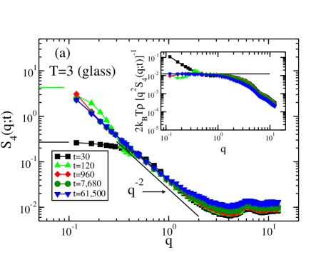
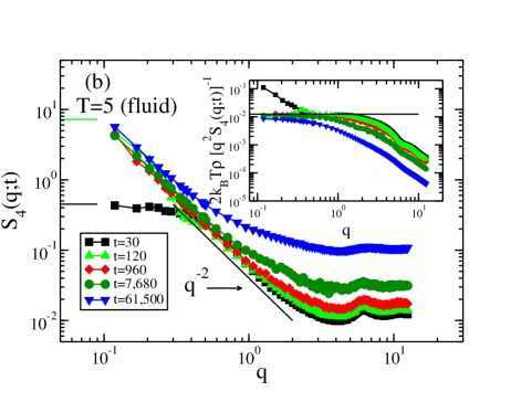
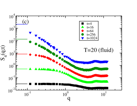
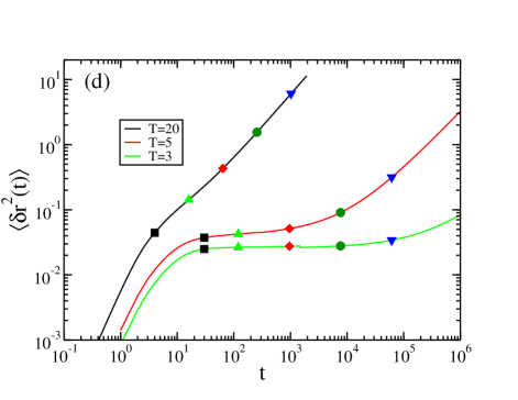
In Fig. 1 we show $S_{4}(q;t)$ at several different times for a glass at $T=3$, a viscous fluid at $T=5$, and a moderate temperature fluid at $T=20$. These times are indicated on the mean square displacement $\left<\delta r^{2}(t)\right>=N^{-1}\left<\sum_{n}\delta\mathbf{r}_{n}^{2}(t)\right>$, which is shown in Fig. 1(d).

Figure 1: (a)-(c) $S_{4}(q;t)$ for a glass at $T=3$ (a), a viscous fluid at $T=5$ (b), and a moderate temperature fluid at T=20 (c). The horizontal lines for $T=3$ and 5 indicate $\chi_{4}(t)=k_{B}Tt^{2}/m$ for $t=30$ and $t=120$. The horizontal lines for $T=20$ indicate $\chi_{4}(t)$ for all the times shown. Note that the oscillations for $T=3$ and 5 at $t=120$ are due to the propagating transverse wave. The inset in (a) and (b) shows $2k_{B}T\rho[S_{4}(q;t)q^{2}]^{-1}$ where the horizontal region is used to calculate the shear modulus $\mu$ of the glass ($T=3$) and the plateau value of the shear stress autocorrelation function of the viscous fluid ($T=5$). In the inset to (a) the continuous horizontal line is the shear modulus calculated from the average of the shear stress autocorrelation function, Fig. 2, between $t=100$ and $10\,000$. In the inset to (b) the continuous horizontal line is the plateau value of the shear stress autocorrelation function, $G_{p}$. The inset in (c) shows the scaling plot of $S_{4}(q;t)/\chi_{4}(t)$ versus $q\xi_{4}(t)$ for $T=20$. The continuous line is the Ornstein-Zernicke function $1/[1+(q\xi_{4})^{2}]$. (d) The mean-square displacement, $\left<\delta r^{2}(t)\right>$, for $T=3,5$ and 20. The circles indicate times at which $S_{4}(q;t)$ is shown in panels (a-c) where the color of the circles correspond to the times shown in panels (a-c). The upturn of $\left<\delta r^{2}(t)\right>$ at the longest times at $T=3$ occurs since our system is aging; with increasing glass annealing time it appears at later and later times. In contrast, the late-time increase of $\left<\delta r^{2}(t)\right>$ at $T=5$ is not subject to aging and does not change with increasing equilibration time.

Figure 2: Shear stress autocorrelation function as a function of time for $T=20$, 15, 12, 10, 8, 7, 6, 5, and 3 listed from left to right. The dashed horizontal line is the shear modulus at $T=3$ obtained from the $2k_{B}T\rho[S_{4}(q;t)q^{2}]^{-1}$ for $t=7680$. The black lines in the main figure are stretched exponential fits to the final decay, $G_{p}\exp\left(-(t/\tau_{\sigma})^{\beta}\right)$. These fits are also are shown in the inset for $T=20$, 15, 12, 10, 8, 7, 6, 5, listed from left to right. The amplitude of the final decay, $G_{p}$, is the same (within error bars) for $T=6$, 5.5 (not shown) and 5. The crosses in the inset are placed at the time when $\xi(t)$ crosses over from linear to $\sqrt{t}$ growth.

We note important limiting behaviors of $S_{4}(q;t)$. First, due to the momentum conservation $\lim_{q\to 0}S_{4}(q;t)\equiv\chi_{4}(t)=k_{B}Tt^{2}/m$ Berthieretal2007 . Second, in the large $q$ limit only the diagonal terms in Eq. (1) contribute and $S_{4}(q;t)=\left<\delta r^{2}(t)\right>/3$.

For the glass $S_{4}(q;t)$ saturates at all the small wave-vectors that we can access in our simulation, Fig. 1a. In the $t\to\infty$ limit $S_{4}(q;t)$ exhibits a $q^{-2}$ divergence indicating power law decay of the correlations in direct space. This behavior of $S_{4}(q;\infty)$ in the glass can be understood using arguments similar to those presented by Klix et al. Klix . Briefly (see the supplemental material for more details), we start with the transverse current $j^{\perp}(\mathbf{q};t)=N^{-1/2}\sum_{n}\mathbf{v}_{n}^{\perp}(t)e^{i\mathbf{q}\cdot\mathbf{r_{n}(t)}}$ where $\mathbf{v}_{n}$ is the velocity of particle $n$, and $\mathbf{v}_{n}^{\perp}$ and $\mathbf{q}$ are chosen such that $\mathbf{v}_{n}^{\perp}\cdot\mathbf{q}=0$. Then, we define a correlation function $\left<\delta\mathbf{u}_{\mathbf{q}}^{\perp}(t)\delta\mathbf{u}_{-\mathbf{q}}^{\perp}(t)\right>$ where $\delta\mathbf{u}_{\mathbf{q}}^{\perp}(t)=\int_{0}^{t}j^{\perp}(\mathbf{q};t)$. It can be shown that $\lim_{q\rightarrow 0}\left<\delta\mathbf{u}_{\mathbf{q}}^{\perp}(t)\delta\mathbf{u}_{-\mathbf{q}}^{\perp}(t)\right>$ is equal to $\lim_{q\rightarrow 0}S_{4}(q;t)$ if the particles displacements are finite; as they are in the glass. Next, we relate $\left<\delta\mathbf{u}_{\mathbf{q}}^{\perp}(t)\delta\mathbf{u}_{-\mathbf{q}}^{\perp}(t)\right>$ to the transverse current correlation function, $C_{t}(q;t)=\left<j^{\perp}(\mathbf{q};t)j^{\perp}(\mathbf{-q};0)\right>$. For the latter function one can derive an exact but formal equation of motion,

$$\frac{dC_{t}(q;t)}{dt}+\int_{0}^{t}M(q;t-s)C_{t}(q;s)ds=0.$$ (2)

In the $q\rightarrow 0$ limit $\rho k_{B}TVq^{-2}M(q;t)$ is equal to the shear stress tensor autocorrelation function $\left<\sigma^{xy}(t)\sigma^{xy}(0)\right>$ comment , see Sec. 9.3 of Ref. simple . Finally, by examining the $t\rightarrow\infty$ limit of $C_{t}(q;t)$ and $\left<\delta\mathbf{u}_{\mathbf{q}}^{\perp}(t)\delta\mathbf{u}_{-\mathbf{q}}^{\perp}(t)\right>$ one can show that $\lim_{q\rightarrow 0}\lim_{t\rightarrow\infty}2k_{B}T\rho[S_{4}(q;t)q^{2}]^{-1}=\lim_{t\rightarrow\infty}\left<\sigma^{xy}(t)\sigma^{xy}(0)\right>/(k_{B}TV)$ if the particle displacements are finite. Since the non-decaying part of $\left<\sigma^{xy}(t)\sigma^{xy}(0)\right>/(k_{B}TV)$ is identified with the glass shear modulus $\mu$ Klix , we obtain the relation $\lim_{q\rightarrow 0}2k_{B}T\rho[S_{4}(q;\infty)q^{2}]^{-1}=\mu$.

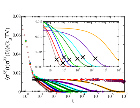
To test this relation we calculated the shear stress autocorrelation function, Fig. 2 (see the supplemental material for details of the calculation). In the fluid, the autocorrelation function exhibits a two-step decay with an intermediate plateau followed by the final structural relaxation. In the glass, there is no final relaxation (on the time scale of the simulation) and this function develops a non-decaying plateau, which is equal to the shear modulus $\mu$.

Using $S_{4}(q;\infty)$ we obtained $\mu=0.013\pm 0.001$, which compares well with the result $\mu=0.012\pm 0.002$ obtained from $\left<\sigma^{xy}(\infty)\sigma^{xy}(0)\right>/(k_{B}TV)$. As an independent check, we used a standard formula for the shear modulus Squire and obtained $\mu=0.010\pm 0.004$. These calculations agree to within error, and similar calculations for the glass at $T=2$ also agree. We emphasize that the $S_{4}(q;\infty)$ calculation is significantly faster than the latter two due to large cancellations involved in the latter calculations. They require simulations that are at least two orders of magnitude longer.

The important difference between our evaluation of the modulus and an earlier calculation of Klix et al. Klix is that our procedure does not require finding average positions of particles during the time $t$. Our four-point structure factor is well-defined both in the glass and the fluid phase and allows one to distinguish between these phases, which is discussed below.

For a viscous fluid there is an intermediate time window where $S_{4}(q;t)$ exhibits features similar to those observed for the glass, Fig. 1b. Specifically, at small wave-vectors we see a $q^{-2}$ dependence of $S_{4}(q;t)$ with an approximately time-independent coefficient. We show in the inset in Fig. 1b that this transient solid-like $q^{-2}$ behavior is related to the transient plateau of the shear stress autocorrelation function. For times within the plateau region and for small wave-vectors $2k_{B}T\rho[S_{4}(q;t)q^{2}]^{-1}$ is equal to $G_{p}$ where $G_{p}$ is the amplitude of the stretched exponential fit to the final decay of $\left<\sigma^{xy}(t)\sigma^{xy}(0)\right>/(k_{B}TV)$.

Finally, at a moderate temperature $S_{4}(q;t)$ increases at all times and wave-vectors, Fig. 1c. Since, the small wave-vector limit of $S_{4}(q;t)$ increases with time faster than does the large wave-vector limit, we should expect that a dynamic correlation length defined through the correlations of transverse displacements diverges in the long-time limit.

To examine the dynamic correlation length we first verify a scaling hypothesis. We assume that there exists a function $f[\cdot]$ such that $S_{4}(q;t)/\chi_{4}(q;t)\approx f[q\xi_{4}(t)]$ where $f(x)=1-x^{2}$ for $x\ll 1$, and $f(x)\sim x^{-2+\sigma}$ for $x\gg 1$. In practice, we determine the dynamic correlation length $\xi(t)$ from the Ornstein-Zernicke fit, $f(x)=1/(1+x^{2})$ for $q\leq 1.0$. In the inset to Fig. 1c we show the excellent data collapse that results by plotting $S_{4}(q;t)/\chi_{4}(q;t)$ versus $\xi_{4}(t)q$, thus confirming the scaling. To find $\sigma$ we fit $S_{4}(q;t)$ for $5\leq x\leq 20$ for $t\geq 1024$ at $T=20$ to $Ax^{-2+\sigma}$ and get $\sigma=-0.23\pm 0.07$.

In Fig. 3 we show $\xi_{4}(t)$ for all $T$. We find a nearly temperature independent initial linear increase in time followed by an increase as $\sqrt{t}$ for later times for $T\geq 6$. At $T=5$ there is a deviation from the linear increase, and we expect that we would observe the $\sqrt{t}$ dependence if we could calculate $S_{4}(q;t)$ for later times, but our system size and simulation length prohibits this calculation. We note that, if calculated at the relaxation time of the fluid (arrows in Fig. 3), which is around the beginning of the $\sqrt{t}$ growth, the lengths shown in Fig. 3 are orders of magnitude larger and increase significantly faster with decreasing temperature than any previously studied four-point correlation lengths.

Figure 3: Time dependence of the dynamic correlation length $\xi_{4}(t)$. The solid line is the linear growth with slope $\sqrt{\mu/(2\rho m)}$ expected for the glass. The shear modulus $\mu$ was obtained from the plateau of the shear stress autocorrelation function for the $T=3$ glass. The dashed lines indicate the $\sqrt{t}$ the growth expected for the fluid at $T=15$, 8 and 6. The arrows indicate the final structural relaxation times of the fluid at the temperatures indicated by the colors.

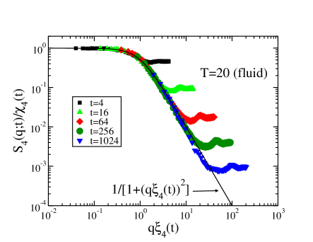
In the glass, the linear growth of $\xi_{4}(t)$ with $t$ is related to the shear modulus. Indeed, in order to get a finite $\lim_{t\to\infty}S_{4}(q;t)$ that is inversely proportional to $q^{2}$ we need $\sigma=0$ and $\xi_{4}(t)\propto t$. Furthermore, the relation between $S_{4}(q;\infty)$ and the modulus allows us to find the coefficient of proportionality and $\xi_{4}(t)=t\sqrt{\mu/(2\rho m)}$. This relation is shown as the solid line in Fig. 3.

We emphasize that particle displacements in the glass are bounded and, therefore, $S_{4}(q;t)$ has a well-defined, finite long-time limit. The long-time divergence of $\xi_{4}(t)$ reflects the presence of long-range correlations that have to accompany rigidity Forster .

In analogy with the glass, in the fluid we find that the initial linear growth of $\xi_{4}(t)$ is related to the transient elastic response, $\xi_{4}(t)\approx t\sqrt{G_{p}/(2\rho m)}$. The subsequent crossover to $\sqrt{t}$ growth should be related to the transient elasticity and the decay of the shear stress autocorrelation function.

The final decay of $\left<\sigma^{xy}(t)\sigma^{xy}(0)\right>/(k_{B}TV)$ is well described by a stretched exponential, $G_{p}\exp[-(t/\tau_{\sigma})^{\beta}]$. The fits are shown as solid lines in Fig. 2. In the inset we show that $G_{p}\exp[-(t/\tau_{\sigma})^{\beta}]$ evaluated at the crossover time (marked by crosses) is almost temperature independent and approximately equal to $0.22G_{p}$. This observation allows us to relate the final long-time behavior of $\xi_{4}(t)$ to the viscosity. Since the final relaxation of the shear stress autocorrelation function is well fit by a stretched exponential, and the viscosity is related to the integral of the shear stress autocorrelation function, then for viscous fluids $\eta\approx G_{p}\tau_{\sigma}\Gamma(1/\beta)/\beta$, where $\Gamma$ is the gamma function (we have ignored the small, short-time contribution to $\eta$). Thus, $\xi_{4}(t)=\sqrt{tg(\beta)\eta/(2\rho m)}$ where $g(\beta)$ is between 1.15 for $\beta=0.5$ and 1.51 for $\beta=1.0$. We show three estimates for final long-time behavior of $\xi_{4}(t)$ in Fig. 3 as dashed lines, where we calculated the viscosity from the shear stress autocorrelation function. For $T\leq 6$, the stretching exponent $\beta$ is constant, thus $g(\beta)$ is independent of temperature and for long times $\xi_{4}(t)=K\sqrt{t\eta}$ where $K$ is a material dependent constant.

We note that, in the fluid, $S_{4}(q;t)$ grows with time without any bound. The divergence of $\xi_{4}(t)$ follows from different small and large wavevector time dependences of $S_{4}(q;t)$. Its connection to fluid’s viscosity is based on an empirical observation and it would be interesting to understand it from a more fundamental perspective.

The above described features of $S_{4}(q;t)$ and $\xi_{4}(t)$ followed from the exact result $\chi_{4}(t)=k_{B}Tt^{2}/m$, which in turn followed from momentum conservation. For a Brownian system, in which the total momentum is not conserved, $\chi_{4}(t)=2D_{0}t$ where $D_{0}$ is the diffusion coefficient of an isolated particle. Preliminary results indicate that in the long time limit, the small $q$ dependence of $S_{4}(q;t)$ for a Brownian glass is identical to that presented here. This is expected since the shear modulus should be a static property of the glass and, thus, independent of the microscopic dynamics. However, for a Brownian fluid we expect that $\xi_{4}(t)\propto\sqrt{t}$ for short times and that $\xi_{4}(t)$ saturates for long times. We note this saturation behavior was found in an earlier study of Doliwa and Heuer DH2000 in which a direct space analogue of $S_{4}(q;t)$ was investigated. However, their study did not connect the time dependence of $\xi_{4}(t)$ to a viscoelastic response.

These findings and preliminary results suggest that other four-point correlation functions used to investigate dynamic heterogeneity contain information about the viscoelastic response of glass-forming fluids and the elastic response of glasses. Indeed, if one uses the microscopic self-intermediate scattering function, $g[\delta\mathbf{r}_{n}(t)]=\exp[-i\mathbf{k}\cdot\delta\mathbf{r}_{n}(t)]$, in Eq. (1) for a fluid system with Newtonian dynamics, one gets a susceptibility with a maximum that increases as the square of the fluid’s relaxation time and a dynamic correlation length that increases as the fluid’s relaxation time. This behavior is a precursor of long-range density correlations that were predicted to exist in the glass due to a spontaneously broken translational symmetry at the microscopic level SFelastic .

Our findings open the way to examine both viscoelastic properties of glass-forming fluids and elasticity of glasses through the analysis of time-dependent particle displacements. This new, general approach requires much less computational effort than the standard approach based on the stress autocorrelation function. It should be especially useful for colloidal systems, in which positions of colloidal particles can be obtained via microscopy but inter-particle interactions are often not well characterized. Finally, this method reveals a direct connection between the viscoelastic response of supercooled liquids and spatially correlated, collective motions of particles.

We gratefully acknowledge the support of NSF grant CHE 1213401. This research utilized the CSU ISTeC Cray HPC System supported by NSF Grant CNS-0923386.

References

- (1) D. Forster, Hydrodynamic fluctuations, Broken Symmetry, and Correlation Functions (Benjamin, Reading, 1975).
- (2) G. Szamel and M. H. Ernst, Phys. Rev. B 48, 112 (1993).
- (3) G. Szamel and E. Flenner, Phys. Rev. Lett. 107, 105505 (2011).
- (4) Dynamical Heterogeneities in Glasses, Colloids, and Granular Media, L. Berthier, G. Biroli, J.-P. Bouchaud, L. Cipelletti, and W. van Saarloos eds. (Oxford University Press, 2011).
- (5) C. Donati, S. Franz, S.C. Glotzer, and G. Parisi, J. Non-Cryst. Solids 307-310, 215 (2002).
- (6) S. Franz, H. Jacquin, G.Parisi, P. Urbani, and F. Zamponi, Proc. Natl. Acad. Sci. U.S.A. 109, 18725 (2012).
- (7) N. Lac̆ević, F.W. Starr, T.B. Schrøder and S.C. Glotzer, J. Chem. Phys. 119, 7372 (2003).
- (8) E. Flenner and G. Szamel, Phys. Rev. Lett. 105, 217801 (2010).
- (9) L. Berthier and T.A. Witten, EPL 86, 10001 (2009).
- (10) E. Flenner and G. Szamel, J. Chem. Phys. 138, 12A523 (2013).
- (11) L. Berthier, G. Biroli, J.-P. Bouchaud, W. Kob, K. Miyazaki, and D.R. Reichman, J. Chem. Phys. 126, 184503 (2007).
- (12) C.L. Klix, F. Ebert, F. Weysser, M. Fuchs, G. Maret, and P. Keim, Phys. Rev. Lett. 109, 178301 (2012).
- (13) We implicitly assume here that for the glass, the shear stress tensor autocorrelation function is continuous as . This assumption is consistent with our simulation results.
- (14) J.-P. Hansen and I.R. McDonald, Theory of Simple Liquids, (Elsevier, 2012).
- (15) D. R. Squire, A. C. Holt, and W. G. Hoover, Physica 42, 388 (1969).
- (16) B. Doliwa and A. Heuer, Phys. Rev. E 61, 6898 (2000).
- (17) See Supplemental Material [url], which includes Refs.lammps ; hoomd ; Yoshino ; Wittmer ; Williams .
- (18) S. Plimpton, J. Comp. Phys. 117, 1 (1995). http://lammps.sandia.gov.
- (19) J.S. Andersen, C.D. Lorenz, and A.Travessef, J. Comp. Phys. 227, 5342 (2008). http://codeblue.umich.edu/hoomd-blue.
- (20) H. Yoshino, J. Chem. Phys. 136, 214108 (2012).
- (21) J.P. Wittmer, H. Xu, P. Polinska, F. Weysser, and J. Baschnagel, J. Chem. Phys. 138, 12A533 (2013).
- (22) S.R. Williams and D.J. Evans, J. Chem. Phys. 132, 184105 (2010).
![[Uncaptioned image]](/html/1405.0442/assets/x7.png)
![[Uncaptioned image]](/html/1405.0442/assets/x8.png)