Logarithmic Spatial Variations and Universal Power Spectra of Temperature Fluctuations in Turbulent Rayleigh-Bénard Convection
Abstract
We report measurements of the temperature variance and frequency power spectrum ( is the distance from the sample bottom and the radial coordinate) in turbulent Rayleigh-Bénard convection (RBC) for Rayleigh numbers and and for a Prandtl number for a sample with a height cm and aspect ratio ( is the diameter). For was consistent with a logarithmic dependence on , and there was a universal (independent of Ra, , and ) normalized spectrum which, for , had the form with a universal constant. Here where is the radius of curvature of the temperature autocorrelation function at . For the measurements yielded with in the range from 3/2 to 5/3. All the results are similar to those for velocity fluctuations in shear flows at sufficiently large Reynolds numbers, suggesting the possibility of an analogy between the flows that is yet to be determined in detail.
pacs:
47.27.-i, 44.25.+f,47.27.TeTurbulent thermal convection is an important phenomenon in many natural processes, for instance in climatology van Doorn et al. (2000), oceanography Marshall and Schott (1999), geophysics Cardin and Olson (1994), astrophysics Busse (1994), and industry. In experiments, it can be generated for instance in a confined system between two horizontal plates separated by a distance and heated from below in the presence of gravity. This system is known as Rayleigh-Bénard convection (RBC) Ahlers (2009); Ahlers et al. (2009a); Lohse and Xia (2010); Chillá and Schumacher (2012).
RBC is frequently studied in a cylindrical sample of height and diameter . Its properties are determined by the Rayleigh number , the Prandtl number , and the aspect ratio . Here is the gravitational acceleration, is the temperature difference between the bottom () and the top () plate, and , , and are, respectively, the thermal expansion coefficient, the kinematic viscosity, and the thermal diffusivity of the fluid.
When Ra is not too large (say ), there are thin laminar boundary layers (BLs) adjacent to the top and bottom plates with most of the temperature difference sustained by them, while the “bulk” of the fluid between these BLs is turbulent. The conventional view was that the bulk is nearly isothermal. This state is known as “classical” RBC. As Ra increases and exceeds a critical value which for is , the shear stress from the turbulent bulk will become sufficiently large to force the BLs into a turbulent state as well and the system enters the “ultimate” state which is expected to be asymptotic as Ra tends toward infinity Kraichnan (1962); Spiegel (1971); Grossmann and Lohse (2011); He et al. (2012).
Recently, it was found that the time-averaged temperature ( is the vertical and the radial coordinate), both in the classical and the ultimate state but outside the BLs, varies logarithmically with the distance from the plates when this distance is not too large (say or so) Ahlers et al. (2012a, 2014). Similar logarithmic behavior is well known from mean velocity profiles of near-wall turbulence in shear flows, such as pipe, channel, and Taylor-Couette flows Wei and Willmarth (1989); Hultmark et al. (2012); Huisman et al. (2013); there it is known as the “Law of the Wall” Prandtl (1925); von Kármán (1930); Prandtl (1932) (for recent reviews, see Marusic et al. (2010); Smits et al. (2011)). For the ultimate state of RBC a logarithmic dependence had been predicted for by Grossmann and Lohse Grossmann and Lohse (2011, 2012). For classical RBC its discovery came as a surprise, but one theoretical explanation was offered very recently She et al. (2014).
In this Letter we report measurements of the temperature variance and of temperature temporal frequency spectra in the bulk of RBC for and which are representative of the phenomena observed in both the classical and the ultimate state. Outside the BLs but in the near-wall range , we found that also varied logarithmically with . The normalized spectra, when scaled by where is the radius of curvature of the time autocorrelation function at , had a universal form (i.e., were independent of Ra, , and ). For they were well described by with a universal constant equal to . Quite remarkably, within our resolution the same universal constant was found in the classical and the ultimate state. To our knowledge, these findings are not explained by present theories for RBC. Away from the near-wall region, near the horizontal midplane of the sample (), we found a universal spectrum with a larger negative exponent close to the Obukhov-Corrsin scaling for a passive scalar in turbulent flows Obukhov (1949); Corrsin (1951). As we show below by using the elliptic approximation (EA) of space-time correlation functions He and Zhang (2006), we find that there is a one-to-one correspondence between the frequency and wave-number domains, thus making it plausible that our findings for the temporal spectra are closely related to the spatial spectra .
The apparatus and the procedures were discussed before Ahlers et al. (2009b, 2012b). The sample was contained in the High Pressure Convection Facility II, a cell of height and diameter m which in turn was located in a very large pressure vessel known as the “Uboot of Göttingen.” The 25 m3 volume of the Uboot and sample were filled with up to 2000 kg of compressed sulfur hexafluoride (SF6) at pressures up to 19 bars as the fluid. By maintaining the mean temperature close to C, Pr was kept at 0.79 (0.86) near (). All measurements had been done under conditions well approximated by the Oberbeck-Boussinesq equations He et al. (2013). The sample was leveled relative to gravity to within rad. In addition to two sets of thermistors that were reported already in Ref. Ahlers et al. (2012a), we installed new thermistors at various vertical and radial locations to measure the interior temperatures (see the Supplementary Material He et al. (2013)).

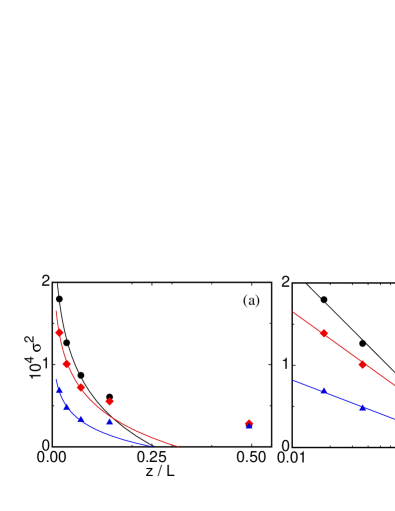
Figure 1 shows vertical profiles of the temperature variance measured at at three different radial positions . For well beyond the thermal BLs (which exist for ) but , all the profiles follow closely a logarithmic dependence on , and can be represented by
| (1) |
As the radial location moves closer to the vertical centerline of the sample, at small decreases while at midheight () it remains the same. This leads to a decease of the amplitude .

| Ra | ( s ) | |||
|---|---|---|---|---|
| 1.080 | 0.0179 | 0.0178 | 0.709 | 0.202 0.014 |
| 1.080 | 0.0362 | 0.0178 | 0.732 | 0.216 0.014 |
| 1.080 | 0.0719 | 0.0178 | 0.801 | 0.216 0.012 |
| 1.080 | 0.1437 | 0.0178 | 0.854 | |
| 1.080 | 0.4933 | 0.0178 | 1.417 | |
| 1.080 | 0.0719 | 0.0357 | 0.829 | 0.210 0.016 |
| 1.080 | 0.0719 | 0.1337 | 0.915 | 0.196 0.015 |
| 1.626 | 0.0179 | 0.0178 | 1.110 | 0.216 0.012 |
| 1.626 | 0.4933 | 0.0178 | 2.051 | |
| 1.626 | 0.0179 | 0.1337 | 1.285 | 0.202 0.018 |
As most (but not all Lohse and Xia (2010)) previous measurements for RBC, we report the temporal behaviour of thermal fluctuations. Based on the elliptic approximation (EA) of space-time cross-correlation functions He and Zhang (2006), there exists an equivalence between spatial and temporal spectra which is exact to second order in the sense that it is based on a systematic second-order expansion of the correlation functions (see the Supplementary Material He et al. (2013)).
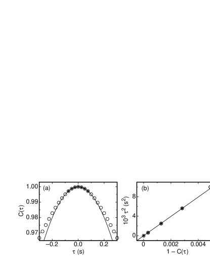
Figure 2 shows a typical temperature autocorrelation function . For , satisfies
| (2) |
Fitting Eq. (2) to the data with the solid dots ( s), we get the characteristic time scales given in Table 1. Here the determination of from is similar to the determination of the Taylor microscale from velocity space autocorrelation functions in turbulent flows Pope (2000).
Elsewhere He et al. (2013) we show that our experimental results for agree well with the EA. An important implication He et al. (2013) is that the temperature space correlation function is equal to provided one chooses . Here with and the mean speed and the root-mean-square velocity, respectively. Similar to , a typical length scale can be derived from the curvature of , and the EA requires that . Therefore the two scaled correlation functions vs and vs are the same. Taking the Fourier transform of both, we have
| (3) |
with . Thus, the normalized spectrum in wave-number space is the same (to second order) as in the frequency domain He et al. (2010), and all arguments regarding the dependence of on apply equally well to the dependence of on . Since our measurements are in the time domain, we shall continue to present our results in the form of , but keep in mind that would have all the same properties.
In the log layer of turbulent shear flows, similarity analysis yielded the prediction Perry and Abell (1977); Perry et al. (1986) that the wave-number spectrum of the velocity should be proportional to in the intermediate wave-number range, and that this dependence on the wave number implies the logarithmic dependence of the velocity variance on position in space. The arguments leading to these results are quite general and one may expect by analogy that they also apply to the temperature variance. As we shall show below, our data are indeed consistent with (or equivalently in the spatial domain ) in the region where we also found that was consistent with a logarithmic dependence on .

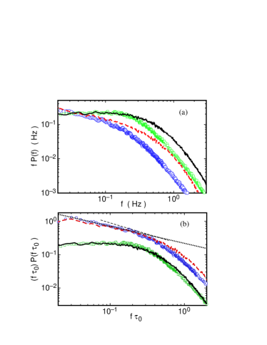
Finally, we turn to experimental results for the spectra. Figure 3 (a) shows compensated normalized temperature frequency power spectra as a function of from measurements at the radial position for two vertical positions: one is in the log layer () and the other is at the sample midheight (). At each position measurements are shown for and , representing the ultimate and the classical state of RBC respectively. One sees that the shape of the spectrum changes with positions as well as with Ra.
Using the value of derived from the autocorrelation function corresponding to each spectrum (see Table 1), we determined the normalized from the spectra in Fig. 3 (a) and plotted the compensated spectra as a function of in Fig. 3 (b). The four spectra now fall into two distinct groups. In the log layer we find a universal spectrum (i.e., independent of Ra) which, over the range , is described well by with and . This observation suggests that the attached-eddy hypothesis of Ref. Townsend (1976) and the similarity argument of Ref. Perry et al. (1986) for near-wall turbulence similarly apply to the RBC bulk temperature (a passive scalar Sun et al. (2006); He et al. (2011)). Elsewhere Ahlers et al. (2014) we discuss in more detail these similarities for the classical state and suggest that the plumes in RBC may play a role similar to the coherent eddies in shear flow, and that the inner length scale given by the viscous sublayer in shear flows (where the coherent eddies originate) is given by the thermal boundary-layer thickness in RBC (where the plumes originate). However, the observed universality persists even though one spectrum is in the classical and the other in the ultimate regime of RBC, and in the ultimate state a different length scale (perhaps that of the thermal sublayer) must prevail.
At midheight, far above the log layer, the experimental spectrum suggests values of near 1.5 or larger, as indicated by the dotted () and dashed () lines in Fig. 3 (b). The value would be consistent with Obukhov-Corrsin scaling for passive scalars Obukhov (1949); Corrsin (1951), and suggests correspondence with experimental findings of Kolmogorov scaling along the center line of turbulent pipe flow Rosenberg et al. (2013). Temperature power spectra have been studied before both by experiment Sano et al. (1989); Procaccia et al. (1991); Cioni et al. (1995); Zhou and Xia (2001) and theory Castaing (1990); L’vov (1991); Lohse (1994) and have yielded values of ranging from to . Our spectrum at midheight is very similar to results from previous studies Niemela et al. (2000); like our data, those results could be interpreted to yield an effective near at low and near at slightly higher frequencies.

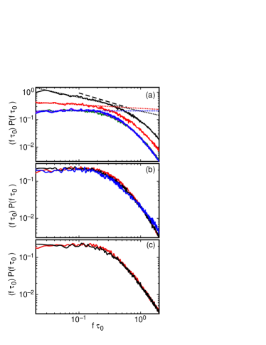
Figure 4 (a) shows compensated spectra for measured at the fixed radial position for varying vertical positions. For the three positions inside the log layer, the spectra again are universal and give for . As increases beyond about , the spectra depart from the universal form and increases beyond the value found in the log layer. At the sample midheight, is in the range of 1.5 (dotted line) to 5/3 (dashed line) as seen before in Fig. 3. For the position between the log layer and the horizontal midplane (red curve), the value of has an intermediate value, suggesting a gradual transition from near-wall turbulence to free turbulence.
Figure 4 (b) shows compensated spectra measured at the fixed height for different radial locations and . In both Figs. 4 (a) and (b), all spectra in the log layer fall on a universal curve independent of position. Figure 4 (c) shows compensated spectra measured at heights for different radial locations measured at . These spectra also collapse onto the same curve as all the others in the log layer, indicating that inside the log layer is universal in the sense that it is independent of both radial and axial positions and of Ra. Remarkably as shown in Table 1, a universal value applies for both the ultimate and the classical state of RBC, if is assumed.
In this Letter we presented the results of a systematic experimental study of the temperature variance and of the spectra in a RBC sample for the ultimate state at and the classical state at . For both states we found that varied logarithmically with near the bottom plate where . The log layer for shares many similarities with the log layer observed in turbulent shear flows such as pipe flow, channel flow, and Taylor-Couette flow Wei and Willmarth (1989); Hultmark et al. (2012); Huisman et al. (2013) (regarding this issue, see also Ahlers et al. (2014)).
On the basis of the elliptic approximation of correlation functions He and Zhang (2006) we discussed that there is an equivalence between frequency spectra and wave-number spectra when frequency is scaled by a time scale based on the curvature of the time autocorrelation function of the temperature and the wave number is scaled by a similarly defined length scale . Thus, predictions for apply equally well to .
For both Ra values, and for all radial and axial positions where the logarithmic dependence of on was found, we found that in the range , with a universal constant equal to . This result, although with its own independent theoretical explanation still missing, shares many similarities with predictions for the wave-number spectrum of velocity fluctuations in the log layer of turbulent pipe flow Perry and Abell (1977); Perry et al. (1986) where the expected dependence remains “elusive” Rosenberg et al. (2013).
Acknowledgements:
We are grateful to the Max-Planck-Society and the Volkswagen Stiftung, whose generous support made the establishment of the facility and the experiments possible. We thank the Deutsche Forschungsgemeinschaft (DFG) for financial support through SFB963: “Astrophysical Flow Instabilities and Turbulence.” The work of G.A. was supported in part by the U.S National Science Foundation through Grant No. DMR11-58514. We thank Andreas Kopp, Artur Kubitzek, Holger Nobach, and Andreas Renner for their enthusiastic technical support.
References
- van Doorn et al. (2000) E. van Doorn, B. Dhruva, K. R. Sreenivasan, and V. Cassella, Phys. Fluids 12, 1529 (2000).
- Marshall and Schott (1999) J. Marshall and F. Schott, Rev. Geophys. 37, 1 (1999).
- Cardin and Olson (1994) P. Cardin and P. Olson, Phys. Earth Planet. Inter. 82, 235 (1994).
- Busse (1994) F. H. Busse, Chaos 4, 123 (1994).
- Ahlers (2009) G. Ahlers, Physics 2, 74 (2009).
- Ahlers et al. (2009a) G. Ahlers, S. Grossmann, and D. Lohse, Rev. Mod. Phys. 81, 503 (2009a).
- Lohse and Xia (2010) D. Lohse and K.-Q. Xia, Annu. Rev. Fluid Mech. 42, 335 (2010).
- Chillá and Schumacher (2012) F. Chillá and J. Schumacher, Eur. Phys. J. E 35, 58 (2012).
- Kraichnan (1962) R. H. Kraichnan, Phys. Fluids 5, 1374 (1962).
- Spiegel (1971) E. A. Spiegel, Ann. Rev. Astron. Astrophys. 9, 323 (1971).
- Grossmann and Lohse (2011) S. Grossmann and D. Lohse, Phys. Fluids 23, 045108 (2011).
- He et al. (2012) X. He, D. Funfschilling, H. Nobach, E. Bodenschatz, and G. Ahlers, Phys. Rev. Lett. 108, 024502 (2012).
- Ahlers et al. (2012a) G. Ahlers, E. Bodenschatz, D. Funfschilling, S. Grossmann, X. He, D. Lohse, R. J. A. M. Stevens, and R. Verzicco, Phys. Rev. Lett. 109, 114501 (2012a).
- Ahlers et al. (2014) G. Ahlers, E. Bodenschatz, and X. He, arXiv:1404.3459 .
- Wei and Willmarth (1989) T. Wei and W. W. Willmarth, J. Fluid Mech. 204, 57 (1989).
- Hultmark et al. (2012) M. Hultmark, M. Vallikivi, S. C. C. Bailey, and A. J. Smits, Phys. Rev. Lett. 108, 094501 (2012).
- Huisman et al. (2013) S. G. Huisman, S. Scharnowski, C. Cierpka, C. J. Kähler, D. Lohse, and C. Sun, Phys. Rev. Lett. 110, 264501 (2013).
- Prandtl (1925) L. Prandtl, Z. Angew. Math. Mech. 5, 136 (1925).
- von Kármán (1930) T. von Kármán, Nachr. Ges. Wiss. Göttingen, Math.-Phys. Kl. 58 (1930).
- Prandtl (1932) L. Prandtl, Ergeb. Aerodyn. Versuch, Göttingen 4, 18 (1932).
- Marusic et al. (2010) I. Marusic, B. J. McKeon, P. A. Monkewitz, H. M. Nagib, A. J. Smits, and K. R. Sreenivasan, Phys. Fluids 22, 065103 (2010).
- Smits et al. (2011) A. J. Smits, B. J. McKeon, and Ivan Marusic, Annu. Rev. Fluid Mech. 43, 353 (2011).
- Grossmann and Lohse (2012) S. Grossmann and D. Lohse, Phys. Fluids 24, 125103 (2012).
- She et al. (2014) Z.-S. She, X. Chen, J. Chen, H.-Y. Zou, Y. Bao, and F. Hussain, arXiv:1401.2138v1 .
- Obukhov (1949) A. M. Obukhov, Izv. Akad. Nauk SSSR, Ser. Geog. Geofiz. 13, 58 (1949).
- Corrsin (1951) S. Corrsin, J. Appl. Phys. 22, 469 (1951).
- He and Zhang (2006) G.-W He and J.-B. Zhang, Phys. Rev. E 73, 055303 (2006).
- Ahlers et al. (2009b) G. Ahlers, D. Funfschilling, and E. Bodenschatz, New J. Phys. 11, 123001 (2009b).
- Ahlers et al. (2012b) G. Ahlers, X. He, D. Funfschilling, and E. Bodenschatz, New J. Phys. 14, 103012 (2012b).
- He et al. (2013) X. He, D. Funfschilling, H. Nobach, E. Bodenschatz, and G. Ahlers, Phys. Rev. Lett. 110, 199401 (2013).
- He et al. (2013) See Supplemental Material for details of the data acquisition, the data analysis, important aspects of the elliptic approximation, and of other discussions relevant to the present paper, which includes Ref. Zhao and He (2009); Kolmogorov (1941); He and Tong (2011); Zhou et al. (2011) .
- Zhao and He (2009) X. Zhao and G.-W. He, Phys. Rev. E 79, 046316 (2009).
- Kolmogorov (1941) A. N. Kolmogorov, CR. Acad. Sci. USSR 30, 299 (1941).
- He and Tong (2011) X. He and P. Tong, Phys. Rev. E 83, 037302 (2011).
- Zhou et al. (2011) Q. Zhou, C.-M. Li, Z.-M. Lu, and Y.-L. Liu, J. Fluid Mech. 683, 94 (2011b).
- Pope (2000) S. B. Pope, Turbulent Flows (Cambridge University Press, Cambridge, England, 2000).
- He et al. (2013) X. He, D. P. M. van Gils, E. Bodenschatz, and G. Ahlers (to be published) .
- He et al. (2010) X. He, G. He, and P. Tong, Phys. Rev. E 81, 065303 (2010).
- Perry and Abell (1977) A. E. Perry and C. J. Abell, J. Fluid Mech. 79, 785 (1977).
- Perry et al. (1986) A. E. Perry, S. Henbest, and M. Chong, J. Fluid Mech. 165, 163 (1986).
- Townsend (1976) A. A. Townsend, The Structure of Turbulent Shear Flow (2nd) (Cambridge University Press, Cambridge, England, 1976).
- Sun et al. (2006) C. Sun, Q. Zhou, and K. Q. Xia, Phys. Rev. Lett. 97, 144504 (2006).
- He et al. (2011) X. He, E. S. C. Ching, and P. Tong, Phys. of Fluids 23, 025106 (2011).
- Rosenberg et al. (2013) B. J. Rosenberg, M. Hultmark, M. Vallikivi, S. C. C. Bailey, and A. J. Smits, J. Fluid Mech. 731, 46 (2013).
- Sano et al. (1989) M. Sano, X. Z. Wu, and A. Libchaber, Phys. Rev. A 40, 6421 (1989).
- Procaccia et al. (1991) I. Procaccia, E. S. C. Ching, P. Constantin, L. P. Kadanoff, A. Libchaber, and X. Z. Wu, Phys. Rev. A 44, 8091 (1991).
- Cioni et al. (1995) S. Cioni, S. Ciliberto, and J. Sommeria, Europhys. Lett. 32, 413 (1995).
- Zhou and Xia (2001) S. Q. Zhou and K.-Q. Xia, Phys. Rev. Lett. 87, 064501 (2001).
- Castaing (1990) B. Castaing, Phys. Rev. Lett. 65, 3209 (1990).
- L’vov (1991) V. S. L’vov, Phys. Rev. Lett. 67, 687 (1991).
- Lohse (1994) D. Lohse, Phys. Rev. Lett. 73, 3223 (1994).
- Niemela et al. (2000) J. J. Niemela, L. Skrbek, K. R. Sreenivasan, and R. Donnelly, Nature 404, 837 (2000).