Growth-induced breaking and unbreaking of ergodicity in fully-connected spin systems
Abstract
Two canonical models of statistical mechanics, the fully-connected voter and Glauber-Ising models, are modified to incorporate growth via the addition or replication of spins. The resulting behaviour is examined in a regime where the timescale of expansion cannot be separated from that of the internal dynamics. Depending on the model specification, growth radically alters the long-time dynamical behaviour by breaking or unbreaking ergodicity.
pacs:
75.10.-b, 05.40.-a, 02.50.Ey1 Introduction
The dynamical behaviour of growing physical systems often involves an interplay between internal dynamics, arising from the interaction rules between the constituent parts, and the mechanism of growth, such as addition, adsorption or replication. Illustrative examples of such systems include the formation of stars and galaxies [1, 2], the growth of cancerous tumours [3, 4] and the ecology of bacterial outbreaks [5]. Existing theoretical work on the subject of growth is, however, largely separated into two specific sub-areas: pure-growth processes, concerned with the time dependence of shape and form, such as directed percolation, diffusion limited aggregation, and Pólya-urn random reinforcement models [6, 7, 8, 9]; and, phase-ordering kinetics, focusing on the scaling of internal dynamical behaviour such as relaxation or coarsening [10, 11, 12]. Neither of these branches fully capture the broad range of dynamical behaviours possible when the timescales of growth and internal dynamics cannot be separated. Such systems comprise a third important class of models, where growth drives the internal dynamics of the system.
In order to better characterise this broad class, we concentrate on highly-idealised, fully-connected, spin- systems; specifically, the voter [13] and Glauber-Ising models [14]. Aside from the fact that these systems are amenable to analytical treatment, the benefit of such an approach is to demonstrate the effects of growth on models whose behaviour at fixed system size is very well understood. Indeed, incorporating a mechanism for the addition or replication of spins strongly affects the long-time behaviour of the magnetization: changing the ergodicity characteristics and the statistics of polarization flips. Under the addition of random spins, the voter model becomes ergodic, with the long-time distribution depending on the rate of growth. Under spin replication dynamics, however, the voter model remains non-ergodic with the statistics of the final state again depending on the rate of growth. By contrast, it appears that growth of any type is sufficient to break ergodicity in the Glauber-Ising model, as the potential wells always become absorbing at long times.
2 Setup
To start, consider a generic fully-connected spin system. In the absence of growth such systems comprise a fixed number of spins , that interact via probabilistic rules for spin ‘flips’. In a typical protocol, spins are updated one at a time, with one unit of time corresponding to spin updates (one ‘Monte-Carlo sweep’). The probability that the system is in a given state at time , evolves according to a master equation [15]. For fully-connected systems, spin flip rates depend only on the magnetization , and the description of the system is reduced to a stochastic jump process in , with jumps of size . For growing systems however, is itself an increasing function of time and therefore the number of spin updates per unit time also increases. The relevant scaling parameter (which must independent of time) is then the initial system size , which provides a lower bound on . With this in mind, such growing systems can be formally examined by expanding the relevant master equation— now modified for the effects of growth— in powers of . The point being that contributions in the resulting expansion describe deterministic internal dynamics for which growth is negligible (i.e., corresponding to the limit ) and higher order terms give corrections that characterise the dominant effects of growth.
For simplicity, we define our growing systems in continuous time. Spins are updated independently, with an average of one update per spin per unit time, in correspondence with the usual Monte-Carlo time in non-growing simulations. The shorthand () is used for the probability that an up (down) spin is flipped, once chosen. At rate , new spins are picked from a reservoir and added to the system. New spins are up with probability , or otherwise down with probability . The probabilities , , and may depend on the magnetization, while the growth rate is generally a function of the system size. The regime of interest is when the timescales of growth and spin flips cannot be separated: that is, when newly added spins interact— but do not equilibrate— with existing spins, before more are added. For this reason, is required to scale like with exponent .
Before writing down the master equation, it should be remarked that to specify the state of a (fully-connected) growing system requires two order parameters, rather than one. The magnetization and the system size comprise one possible choice; here, the pair is used instead, where and are the total number of up and down spins, respectively. These variables have the advantage that their change is measured in constant steps of , unlike magnetization, whose step-size gets smaller as the system gets larger. The master equation is
| (1) | |||||
where we have made use of step operators with action , for a generic function . For small values of the step increment , this action is well-approximated by Taylor series, since . This allows for the expansion of the master equation for large in a standard way [15]. Neglecting terms, a Fokker-Planck equation is obtained from (1) that is equivalent to the following Langevin pair:
| (2) | |||||
| (3) |
where is a single source of standard Gaussian white noise, understood in the Itō sense. Note: whilst Langevin equations are preferred for clarity of discussion, we make repeated use of the fact that a stochastic variable obeying the (Itō) Langevin equation has probability density obeying for the Fokker-Planck equation , see [20] for proof.
Equations (2) and (3) underpin the main results of this paper, describing the evolution of a fully-connected spin-system growing from an initial size . Their key aspects can be better understood by first transforming to a description in terms of the scale and magnetization . The spin flip and noise terms in (2) and (3) cancel to produce deterministic dynamics for scale,
| (4) |
while the magnetization remains stochastic,
| (5) |
We now see that growth modifies the dynamics of magnetization by i) introducing a weak deterministic pull towards the magnetization of the reservoir, and ii) continually reducing the magnitude of the stochastic fluctuations. These apparently minor modifications can have a profound impact on the dynamics, as illustrated by two classic examples of interacting spin-systems: the voter and Glauber-Ising models.
3 Growing voter model
Attractive as a theoretical tool because of its lack of free-parameters, the surprisingly rich dynamics of the voter model arise from a simple update mechanism in which spins copy the state of a randomly selected neighbour. In the fully-connected case, the flip probabilities are and , which leads to the cancellation of the first two terms in (5). For non-growing systems (, ) the dynamical behaviour is then straightforward: the possible states are explored by a random walk in , which halts when one of the two absorbing polarized states () are reached. This model system is non-ergodic; the time average of a single realisation will concentrate on just one of the polarized states, whereas the ensemble average will sample both with equal probability.
Things are very different when the effects of growth are included. For example, suppose the system is coupled to an unmagnetized reservoir () from which spins are added at a constant rate . With no deterministic contribution, the equation for magnetization (5) can be decoupled from by introducing a rescaled time satisfying
| (6) |
Under constant growth Eq. (4) gives , which implies . In rescaled time (5) becomes
| (7) |

The behaviour described by this equation is that of noise-induced bistability (that is, the addition of noise changes the dynamics from mono- to bistable, see e.g., [16, 17]). The noise is largest at when the deterministic pull is zero and vice-versa at the boundaries . In the long-time limit, the probability distribution of the magnetization converges to the stationary solution of the corresponding Fokker-Planck equation. In this case,
| (8) |
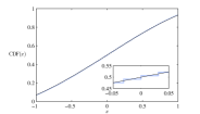
Although the distribution diverges at , these are no longer absorbing states, but have instead become metastable in the sense that transitions between them are rare. To quantify this observation, we examine the statistics of the first-passage time taken to move from one polarized state to the other. Here, the probability distribution of first-passage time obeys the backward Fokker-Planck equation corresponding to (7), but with a reflecting barrier placed at the start point and an absorbing barrier at the destination [20]. It was shown in [18] that the process defined by (7) has the first-passage time distribution , where denotes the derivative of the elliptic theta function of the first kind [19] with respect to the first argument. Undoing the time rescaling, we find
| (9) |
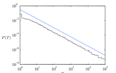
In particular, although is almost surely finite, it has infinite mean, and series expansion (see [19]) reveals a tail that decays as a power law . This prediction is verified in continuous-time Monte-Carlo (Gillespie algorithm) simulations of the fully-connected voter model growing due to accretion of random spins, see Fig. 1.
In the above example, the constant accretion of spins with random sign turned the voter model into an ergodic system by destroying its absorbing states. However, this behaviour is not shared by another natural mechanism for system growth: replication. For example, suppose that the sign of newly added spins is determined by sampling from the existing system, so that and . In this case, the same time-rescaling as before can be applied [Eq. (6)], resulting in the autonomous equation
| (10) |
which recovers the known dynamics of a voter model of fixed size . According to this equation, the system will eventually become trapped in one of the two absorbing states . Thus the growing system remains non-ergodic, in contrast to the case of growth due to the accretion of randomly aligned spins. If the initial magnetization is zero then both possible final states are equally likely, and .


The treatment of growing voter models may be further generalised to cases where is not only increasing, but accelerating. Within our framework, this is realised by a growth rate , where . Such situations arise, for example, in the case where growth is proportional to some surface area, e.g., imagine a growing -dimensional ball of spins, so that . (Note that regardless of spatial organisation the present analysis is still restricted to infinite range systems, i.e., those that are fully-connected). If the sign of the incoming spins is random, the result it trivial: the deterministic pull towards the magnetization of the reservoir is stronger than the noise [since in Eq. (5)], and the system becomes a deterministic reflection of the reservoir in the limit. However, for the case of replicating spins, the third term of (5) vanishes and the time-rescaling (4) can be used once again. Here, solving (4) for , substituting into the right-hand side of (6) and integrating, gives
| (11) |
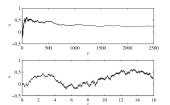
which has a finite limit , as . This means that the dynamics of the accelerating voter model (with replication) slow asymptotically to a halt, and the probability distribution of final states is given by the corresponding autonomous (fixed size, rescaled-time) system, frozen at time . Indeed, the autonomous system in this case is precisely that described by (7), i.e., the non-growing counterpart (of size ) of the accelerating system. Monte-Carlo simulations presented in Fig. 2 show example results for a growing disc () with replicating surface-spins. Table 1 contains a summary of the four different possible growing voter model regimes.
| Accretion () | Replication (, ) | |
|---|---|---|
| Constant growth | ||
| ergodic | non-ergodic | |
| Accelerating growth | ||
| deterministic | non-ergodic |
4 Growing Glauber-Ising model
The symmetries of the voter model make it somewhat special in that its dynamics are driven entirely by stochastic fluctuations. What are the effects of growth in more general systems described by motion in a potential? To answer this question we analyse another canonical model of interacting spins, the fully-connected Glauber-Ising model [14] (equivalently, the Curie-Weiss model with Glauber dynamics). Here, the statistical weight assigned to each state is proportional to where is inverse temperature and specifies the Hamiltonian, with coupling strength and external magnetic field . Under Glauber dynamics, the flip rates are given by and [14], such that the dynamics of finite, non-growing, systems are described by stochastic motion in the potential
| (12) |
with multiplicative noise specified by state-dependent diffusion
| (13) |
In particular, the limit of Eq. (5) describes the deterministic dynamics
| (14) |
This contrasts with the voter model, which has a flat potential and therefore no contribution to the dynamics. The presence of a non-flat potential rules out decoupling and by rescaling time. Nevertheless, it is still possible to calculate statistical properties of system trajectories.

The non-growing Glauber-Ising model does not possess any absorbing states (in long times it samples the equilibrium distribution), however, below the critical temperature a pair of metastable states develop with opposite polarization, corresponding to minima of the potential . This prompts an investigation of these states in the growing system, focusing again on the first-passage time to move from one potential well to the other. Inspired by Kramer’s method [20], a separation of timescales between two types of phase-space trajectory may be exploited; trajectories that travel between points within the same potential well are considered much more frequent than those which cross the potential barrier. Under this assumption, it is then reasonable to introduce a size-dependent instantaneous escape rate , found as the reciprocal of the mean first-passage time for fixed system size . This quantity can be computed via steepest descent.
Writing for the location of the starting well (without loss of generality we choose the left-hand well) and for the location of the potential maximum between wells, we have
| (15) |
We erect a reflecting barrier at and an absorbing barrier at some . Introducing
| (16) |
the mean first-passage time from to with fixed is given by [20]
| (17) |
For large , the inner integral here is dominated by behaviour near and the outer by behaviour near . By Laplace’s method we may approximate
| (18) |
From the definition (16) we compute , but and are both turning points of , so the second term vanishes there. Under the assumption that the dynamics are approximately memoryless, the instantaneous escape rate is given by the reciprocal of the mean first-passage time at fixed size. From the above calculation we obtain
| (19) |
The statistics of the first-passage time of the growing system are captured by the survivor function, giving the probability that the system has not escaped the starting well before time , which is expressed in terms of by
| (20) |
For the case of constant growth , which, when substituted into (20), gives
| (21) |
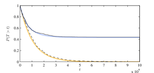
where and are constants depending on . In particular, we find a finite probability that the growing system may never leave the starting well: . This is in contrast to the non-growing case, which always escapes eventually. Figure 3 contains a numerical demonstration of this dichotomy. Moreover, even if the growing system succeeds in switching wells once, the probability of switching back is even smaller (this can be seen by repeating the analysis with as the system size after the first switch). Eventually, the growing Glauber-Ising model is sure to become stuck in one well, thus breaking ergodicity.
5 Discussion
In summary, our theoretical analysis demonstrates that the interplay between growth and relaxation can dramatically change the behaviour of even the simplest of systems. We have seen how the canonical fully-connected voter and Glauber-Ising models respond quite differently to growth due to constant accretion of random spins. The fully polarized states of the voter model cease to be absorbing, while the metastable minima of the Glauber-Ising model eventually become absorbing as time goes on. A third type of behaviour was found in the voter model undergoing surface growth due to replication, where the system state converges to that of a non-growing system frozen at a finite time. These results make clear the power of growth as a mechanism for driving systems away from equilibrium. Looking forward, one particularly interesting area of application lies in the field of population genetics. The fully-connected voter model is very closely related to the Wright-Fisher [21, 22] and Moran [23] models of genetic drift, in which case Table 1 describes the possible long-time genetic profiles of growing populations.
Finally, we have focused here on models with infinite magnetic interaction range. The next step in the development of this new field will be the treatment of finite-range spatially heterogeneous systems (such as that found in recent experimental studies [24] of growing Bacterial colonies), where we can expect to uncover further novel phenomena driven by growth.
Acknowledgements. TR thanks Robert Jack and Nigel Wilding for useful discussion. RGM thanks George Rowlands for useful discussion, and acknowledges funding from EPSRC grant EP/E501311/1.
References
References
- [1] E. Kolb and M. S. Turner, The early universe (Addison-Wesley, San-Francisco, 1990).
- [2] A. Berera and L.-Z. Fang, Phys. Rev. Lett. 72, 458 (1994).
- [3] D. Hanahan and R. A. Weinberg, Cell 100, 57 (2000).
- [4] N. Beerenwinkel et al., PLoS Comput. Biol. 3, e225 (2007).
- [5] S. R. Harris et al., Science (New York, N.Y.) 327, 469 (2010).
- [6] H. Herrmann, Phys. Rep. 136, 153 (1986).
- [7] F. Family and T. Viscek, Dynamics of fractal surfaces (World Scientific Publishing, Singapore, 1991).
- [8] M. Marsili, A. Maritan, F. Toigo, and J. Banavar, Rev. Mod. Phys. 68, 963 (1996).
- [9] R. Peamantle, Probability Surveys 4, 1–79 (2007)
- [10] H. Furukawa, Adv. Phys. 34, 703 (1985).
- [11] A. Bray, Adv. Phys. 43, 357 (1994).
- [12] D. I. Russell and R. A. Blythe, Phys. Rev. Lett. 106, 16 (2011).
- [13] T. M. Liggett, Stochastic interacting systems: contact, voter and exclusion processes (Springer-Verlag, Berlin, 1999).
- [14] P. L. Krapivsky, S. Redner, and E. Ben-Naim, A kinetic view of statistical physics (Cambridge University Press, Cambridge, 2010).
- [15] N. G. van Kampen, Stochastic processes in physics and chemistry (Elsevier, Amsterdam, 1992).
- [16] T. Biancalani, T. Rogers, and A. J. McKane, Phys. Rev. E 86, 010106 (2012).
- [17] T. Biancalani, L. Dyson, and A. J. McKane, Phys. Rev. Lett. 112, 038101 (2014).
- [18] T. Biancalani, Ph.D. thesis, Chapter 3, The University of Manchester, 2013.
- [19] J. V. Armitage and W. F. Eberlein, Elliptic Functions, 1st ed. (Cambridge University Press, Cambridge, 2006).
- [20] C. Gardiner, Handbook of stochastic methods (Springer-Verlag, Berlin, 1985).
- [21] R. A. Fisher, The Genetical Theory of Natural Selection (Clarendon, Oxford, 1930).
- [22] S. Wright, Genetics 16 97 (1931).
- [23] P. A. P. Moran, Proc. Camb. Phil. Soc. 54 60 (1958).
- [24] O. Hallatschek, P. Hersen, S. Ramanathan, and D. R. Nelson, Proc. Nat. Ac. Sci. 104 50 (2007).