Aligned Natural Inflation:
Monodromies of two Axions
Rolf Kappl, Sven Krippendorf and Hans Peter Nilles
Bethe Center for Theoretical Physics
and
Physikalisches Institut der Universität Bonn
Nussallee 12, 53115 Bonn, Germany
kappl, krippendorf, nilles at th.physik.uni-bonn.de
Abstract
Natural (axionic) inflation [1] can accommodate sizeable primordial tensor modes but suffers from the necessity of trans-Planckian variations of the inflaton field. This problem can be solved via the mechanism of aligned axions [2], where the aligned axion spirals down in the potential of other axions. We elaborate on the mechanism in view of the recently reported observations of the BICEP2 collaboration [3].
![[Uncaptioned image]](/html/1404.7127/assets/x1.png)
The motion of the inflaton:
The aligned axion roles down in the valley of a second axion.
1 Introduction
Natural inflation [1, 4] is one of the best motivated scenarios to describe the inflationary expansion in the early universe. The flatness of the potential is protected by a (shift) symmetry modelled after the QCD axion [5], although at different mass scales. The axion exhibits a shift symmetry that is perturbatively exact, but potentially broken by non-perturbative (instantonic) effects. In its simplest form [1] natural (axionic) inflation is derived from the potential
| (1) |
where is the axion decay constant and is the overall scale of the potential. This is a periodic potential with period . If inflation occurs for field values this coincides with chaotic inflation [6] in its quadratic form . Axions are well motivated also in the framework of string theory and its various antisymmetric tensor fields. Their specific properties as pseudoscalar fields allow a wide spectrum of potential applications in particle physics and cosmology (see for instance [7]).
With the recent observation of the BICEP2 experiment [3], axionic inflation returned to the focus of the discussion [8], as it allows sizeable tensor modes up to a value of . The results of BICEP2 point to a value of (after dust reduction to ), a much higher value than expected compared to the results obtained by the Planck satellite [9]. More observations are needed to determine the precise value for . Up to now the results seem to be compatible with the prediction of axionic inflation.
One general aspect of inflationary models with large tensor modes is the appearance of trans-Planckian values of the inflaton field known as the Lyth bound [10, 11]. For example, the model of quadratic inflation with sufficient number of e-folds requires the displacement , where . We thus have to worry whether our low energy effective description based on classical gravity is still valid under these circumstances. Quantum gravitational effects might destroy the properties of the inflationary potential.
This is a generic problem of all models with “large” tensor modes and we have to find arguments to assure the flatness of the potential even at trans-Planckian values of the field. In absence of a complete theory of quantum gravity this is a severe problem. Axionic inflation has an ingredient that helps in this direction: its shift symmetry might be respected by such effects. This is supported by string theoretic arguments through the appearance of (discrete) gauge symmetries that survive in the ultra-violet completion [12, 13, 14, 15, 16].
In that sense, axionic inflation appears as the most attractive scenario to avoid the problems of trans-Planckian field values, although these questions have to be analysed on a case by case basis.111Discrete symmetries in string constructions have been discussed for example in refs. [17, 18, 15, 19, 20, 21, 22, 23, 24, 25, 26, 27, 28].
So let us concentrate on axionic inflation. Unfortunately we still have to face some problems. In the potential (1), trans-Planckian values of the inflation field require . In fact, in the region of high tensor modes we obtain and this poses a severe problem. Within the framework of string theory we expect to be at most as large as the string scale [29, 30, 31].222Because of the rather high value of the observed tensor modes we expect large values for the potential and a rather high value of the string scale as well. Values of and larger than would lead us to the uncontrollable regime of strongly interacting string theory where a meaningful discussion of the flatness of a potential will be impossible. A simple picture of axionic inflation with a single axion and potential (1) is therefore problematic.
As we have discussed earlier, string theory might provide various axion candidates, we would have the option to consider models with various axions, and this is what we want to explore in this paper. We shall follow the suggestion of ref. [2] of axionic inflation with aligned axions: one axion spiralling down in the valley of a second one (see Figure 2 and its copy on the title page). This mechanism encodes all the nice features of schemes later called “axion monodromy” [32, 33] in a somewhat different set-up (see also [34] for an overview on axion inflation). The alternative suggestion of many non-interacting axions, N-flation [35] differs significantly from the mechanism described here. In addition it requires a really large number of axion fields [36] that might be problematic in an explicit realisation. We shall comment on these mechanisms later in this paper (Section 3).
2 A two axion field theoretical realisation
To illustrate axionic inflation with aligned axions, let us recall the realisation presented by Kim, Nilles and Peloso in [2]. We start with the following two field model
| (2) | |||||
| (3) |
Here we introduce no different energy scales for the cosine factors, which do not alter the results of our following discussion. There is a flat direction in this potential, if the following relation holds
| (4) |
This can be seen by looking at the two mass eigenvalues near the origin ()
| (5) |
where the last term under the square root simplifies to zero if relation (4) holds and one eigenvalue remains zero.
We are interested in breaking this flat direction by the small parameter which we define as follows:
| (6) |
We would like to utilise this flat direction for inflation, while keeping the other direction fixed. More precisely, we are interested in obtaining inflation near the origin. A visualisation of the potential with a universal decay constant and the flat direction can be found in Figure 1 which shows the potential for various values of
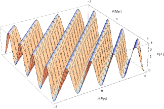
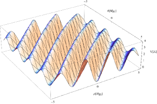
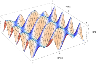
The first step to analyse inflation, is to go into a suitable basis which parametrises our inflationary trajectory. To set notation we introduce the following new coordinates:
| (7) |
where parametrises the flattest direction in the potential around the origin and its orthogonal direction. This flattest direction is given by the smallest eigenvalue of the Hessian of the potential in (3) (see equation (5)). Let us denote the eigenvectors of the Hessian by and with corresponding to the smaller eigenvalue The transformation is then explicitly given by
| (8) |
where with and denotes the matrix out of eigenvectors. The normalisation of this transformation is chosen that the new basis has canonical kinetic terms. The inverse transformation is given by
| (9) |
Note that this field transformation as of now has been model-independent and it can be applied to other models with similar flat directions. Now, turning to the field theoretical model in (2) with the approximation as in (6), we find the following expressions for the transformation up to first order in
| (14) | |||||
| (19) |
We are interested in parameter ranges in the above potential (3) which are suitable for inflation. Here we focus on generating inflation along the ‘flat’ direction parametrised by in the neighbourhood of the origin. To analyse the inflationary foot-prints of this particular single field model, let us re-write the potential as follows:
| (20) |
The coefficients are to first order in given by:
| (21) | |||||
| (22) |
The leading order expansion in matches with the expansion of a potential as in natural inflation
| (23) |
where the effective decay constant is given by
| (24) |
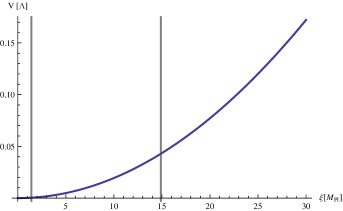
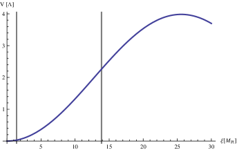
We see that by aligning the decay constants appropriately an arbitrarily large effective decay constant can be arranged. A visualisation of the potential along the inflaton direction is shown in Figure 2 where we parametrise the -coordinates by and to visualise the axionic shift symmetries in the and directions.
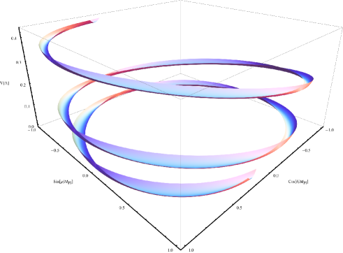
In this model, the slow-roll parameters are then found to be:
| (25) | |||||
| (26) | |||||
| (27) | |||||
| (28) |
In the respective last lines we provide the leading order expressions in the expansions of and around zero.
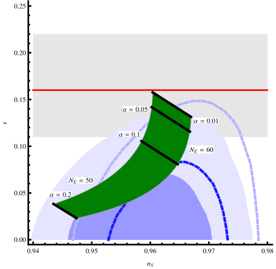
Equipped with these slow-roll parameters, we can now determine the model footprint in the plane. The result is shown in Figure 3 for varying values of the expansion parameter Note that by varying the other parameters and the model footprint remains the same. We find that the footprint is very similar to the one of natural inflation (e.g. [8]). As outlined in recent analysis on natural inflation, this is a very attractive area of parameter space in the light of the recent BICEP2 observation of tensor modes. Note also that the same region of natural inflation can be achieved by bottom-up extensions of natural inflation (see for instance the recent papers [37, 38, 39]).
3 Discussion
We have seen that the mechanism of aligned axions solves the problem of “trans-Planckian” field values and thus completes the scenario of natural (axionic) inflation [2]. It is characterised by a new parameter that measures the amount of alignment ( corresponds to full alignment). A precise measurement of the tensor mode ratio would allow us to determine (within this scheme) a narrow range for the value of (see Figure 3). Natural inflation is limited to and for these values of has to be small. Values of would correspond to , a rather light alignment. Therefore we are confident that such values can be achieved in explicit models without a strongly fine-tuned value of .
Before we enter the details of potential model building let us comment on some alternative suggestions for the solution of the trans-Planckian problem. One of them is so-called N-flation [35], motivated by the mechanism of assisted inflation [40]. It should not be confused with the alignment mechanism discussed in this paper as it suggests the existence of non-interactive axions. With such a setup one can construct an effective axion scale (with individual scales ). In a realistic setting this mechanism requires many axions (see for instance [36, 41, 42]). The existence of many fields leads to a renormalisation of the Planck scale proportional to as well and it is not clear whether could keep up with the “increase” of the Planck-mass.
Other suggestions for a solution of the trans-Planckian problem use mechanism very similar to the alignment mechanism of KNP [2]. They are based on axionic fields in specific brane backgrounds motivated from string theory [43, 32, 33, 44, 45, 46, 47, 48] and in F-theory [49, 50]. These brane backgrounds (as e.g. NS5-branes) break the axionic symmetries explicitly and provide a slope for the axion to slide down. With this breakdown of the axionic symmetry one might worry whether the original shift symmetry still protects trans-Planckian displacements. The effect of brane-backreactions might be too strong for the mechanism to survive [51, 42]. The original shift symmetry might thus not suffice to guarantee the flat potential needed for inflation. More work needs to be done to see whether these scenarios really solve the trans-Planckian problem (see [52, 53] for alternative approaches). A scheme known as “Dante’s Inferno” [54] considers a two-axion scheme as in [2] and adds a background brane to tilt the potential. As this brane might lead to uncontrollable backreactions as well, it might also be counterproductive to a solution of the trans-Planckian problem.
Of course, we do not yet have an explicit incorporation of the aligned axion scenario in string theory, but we think it is worthwhile to invest some work in this direction. In the original approach [2] one was considering the axions from the NS-NS two form in the heterotic string with a breakdown of the shift symmetry through gauge instantons. There it was rather difficult to obtain a small value of . As is known by now, the NS-NS axions might also lead to a so-called -problem through moduli mixing in the Kähler potential (see for instance [42]). At this point it seems that the -axions for instance from the R-R two form might be better suited for our purpose. There are various effects that break the shift symmetries in a controllable way, that might allow for realistic values of the alignment parameter without specific fine-tuning. In any case, let us first wait for a more precise measurement of the value of that determines the required value of .
Note added
During our work on the alignment mechanism we became aware of other work that might be relevant in this direction. In [55], the authors discuss extensions of the KNP-mechanism with more than two axions, which can help to ameliorate the potential fine-tuning in In [56], the embedding of natural inflation in supergravity is discussed based on earlier work in the framework of supergravity shift symmetries (see for instance [57, 58, 59, 60]).
Acknowledgements
This work was supported by the SFB-Transregio TR33 “The Dark Universe” (Deutsche Forschungsgemeinschaft).
References
- [1] K. Freese, J. A. Frieman, and A. V. Olinto, “Natural inflation with pseudo - Nambu-Goldstone bosons,” Phys.Rev.Lett. 65 (1990) 3233–3236.
- [2] J. E. Kim, H. P. Nilles, and M. Peloso, “Completing natural inflation,” JCAP 0501 (2005) 005, arXiv:hep-ph/0409138 [hep-ph].
- [3] BICEP2 Collaboration Collaboration, P. Ade et al., “BICEP2 I: Detection Of B-mode Polarization at Degree Angular Scales,” arXiv:1403.3985 [astro-ph.CO].
- [4] F. C. Adams, J. R. Bond, K. Freese, J. A. Frieman, and A. V. Olinto, “Natural inflation: Particle physics models, power law spectra for large scale structure, and constraints from COBE,” Phys.Rev. D47 (1993) 426–455, arXiv:hep-ph/9207245 [hep-ph].
- [5] R. Peccei and H. R. Quinn, “CP Conservation in the Presence of Instantons,” Phys.Rev.Lett. 38 (1977) 1440–1443.
- [6] A. D. Linde, “Chaotic Inflation,” Phys.Lett. B129 (1983) 177–181.
- [7] A. Chatzistavrakidis, E. Erfani, H. P. Nilles, and I. Zavala, “Axiology,” JCAP 1209 (2012) 006, arXiv:1207.1128 [hep-ph].
- [8] K. Freese and W. H. Kinney, “Natural Inflation: Consistency with Cosmic Microwave Background Observations of Planck and BICEP2,” arXiv:1403.5277 [astro-ph.CO].
- [9] Planck Collaboration Collaboration, P. Ade et al., “Planck 2013 results. XXII. Constraints on inflation,” arXiv:1303.5082 [astro-ph.CO].
- [10] D. H. Lyth, “What would we learn by detecting a gravitational wave signal in the cosmic microwave background anisotropy?,” Phys.Rev.Lett. 78 (1997) 1861–1863, arXiv:hep-ph/9606387 [hep-ph].
- [11] D. H. Lyth, “BICEP2, the curvature perturbation and supersymmetry,” arXiv:1403.7323 [hep-ph].
- [12] O. Lebedev, H. P. Nilles, S. Raby, S. Ramos-Sanchez, M. Ratz, et al., “The Heterotic Road to the MSSM with R parity,” Phys.Rev. D77 (2008) 046013, arXiv:0708.2691 [hep-th].
- [13] R. Kappl, H. P. Nilles, S. Ramos-Sanchez, M. Ratz, K. Schmidt-Hoberg, et al., “Large hierarchies from approximate R symmetries,” Phys.Rev.Lett. 102 (2009) 121602, arXiv:0812.2120 [hep-th].
- [14] H. P. Nilles, S. Ramos-Sanchez, M. Ratz, and P. K. Vaudrevange, “From strings to the MSSM,” Eur.Phys.J. C59 (2009) 249–267, arXiv:0806.3905 [hep-th].
- [15] M. Berasaluce-Gonzalez, L. E. Ibanez, P. Soler, and A. M. Uranga, “Discrete gauge symmetries in D-brane models,” JHEP 1112 (2011) 113, arXiv:1106.4169 [hep-th].
- [16] J. E. Kim, “The inflation point in U(1)de hilltop potential assisted by chaoton, BICEP2 data, and trans-Planckian decay constant,” arXiv:1404.4022 [hep-ph].
- [17] T. Kobayashi, H. P. Nilles, F. Ploger, S. Raby, and M. Ratz, “Stringy origin of non-Abelian discrete flavor symmetries,” Nucl.Phys. B768 (2007) 135–156, arXiv:hep-ph/0611020 [hep-ph].
- [18] K.-S. Choi, H. P. Nilles, S. Ramos-Sanchez, and P. K. Vaudrevange, “Accions,” Phys.Lett. B675 (2009) 381–386, arXiv:0902.3070 [hep-th].
- [19] H. P. Nilles, M. Ratz, and P. K. Vaudrevange, “Origin of Family Symmetries,” Fortsch.Phys. 61 (2013) 493–506, arXiv:1204.2206 [hep-ph].
- [20] L. Ibanez, A. Schellekens, and A. Uranga, “Discrete Gauge Symmetries in Discrete MSSM-like Orientifolds,” Nucl.Phys. B865 (2012) 509–540, arXiv:1205.5364 [hep-th].
- [21] M. Berasaluce-Gonzalez, P. Camara, F. Marchesano, D. Regalado, and A. Uranga, “Non-Abelian discrete gauge symmetries in 4d string models,” JHEP 1209 (2012) 059, arXiv:1206.2383 [hep-th].
- [22] M. Berasaluce-Gonzalez, P. Camara, F. Marchesano, and A. Uranga, “Zp charged branes in flux compactifications,” JHEP 1304 (2013) 138, arXiv:1211.5317 [hep-th].
- [23] P. Anastasopoulos, M. Cvetic, R. Richter, and P. K. Vaudrevange, “String Constraints on Discrete Symmetries in MSSM Type II Quivers,” JHEP 1303 (2013) 011, arXiv:1211.1017 [hep-th].
- [24] G. Honecker and W. Staessens, “To Tilt or Not To Tilt: Discrete Gauge Symmetries in Global Intersecting D-Brane Models,” JHEP 1310 (2013) 146, arXiv:1303.4415 [hep-th].
- [25] F. Marchesano, D. Regalado, and L. Vazquez-Mercado, “Discrete flavor symmetries in D-brane models,” JHEP 1309 (2013) 028, arXiv:1306.1284 [hep-th].
- [26] J. E. Kim, “Abelian discrete symmetries and from string orbifolds,” Phys.Lett. B726 (2013) 450–455, arXiv:1308.0344 [hep-th].
- [27] M. Berasaluce-Gonz lez, G. Ram rez, and A. M. Uranga, “Antisymmetric tensor gauge symmetries in field theory and string theory,” JHEP 1401 (2014) 059, arXiv:1310.5582 [hep-th].
- [28] H. P. Nilles and P. K. S. Vaudrevange, “Geography of Fields in Extra Dimensions: String Theory Lessons for Particle Physics,” arXiv:1403.1597 [hep-th].
- [29] K. Choi and J. E. Kim, “Harmful Axions in Superstring Models,” Phys.Lett. B154 (1985) 393.
- [30] T. Banks, M. Dine, P. J. Fox, and E. Gorbatov, “On the possibility of large axion decay constants,” JCAP 0306 (2003) 001, arXiv:hep-th/0303252 [hep-th].
- [31] P. Svrcek and E. Witten, “Axions In String Theory,” JHEP 0606 (2006) 051, arXiv:hep-th/0605206 [hep-th].
- [32] E. Silverstein and A. Westphal, “Monodromy in the CMB: Gravity Waves and String Inflation,” Phys.Rev. D78 (2008) 106003, arXiv:0803.3085 [hep-th].
- [33] L. McAllister, E. Silverstein, and A. Westphal, “Gravity Waves and Linear Inflation from Axion Monodromy,” Phys.Rev. D82 (2010) 046003, arXiv:0808.0706 [hep-th].
- [34] E. Pajer and M. Peloso, “A review of Axion Inflation in the era of Planck,” Class.Quant.Grav. 30 (2013) 214002, arXiv:1305.3557 [hep-th].
- [35] S. Dimopoulos, S. Kachru, J. McGreevy, and J. G. Wacker, “N-flation,” JCAP 0808 (2008) 003, arXiv:hep-th/0507205 [hep-th].
- [36] S. A. Kim and A. R. Liddle, “Nflation: multi-field inflationary dynamics and perturbations,” Phys.Rev. D74 (2006) 023513, arXiv:astro-ph/0605604 [astro-ph].
- [37] M. Czerny, T. Higaki, and F. Takahashi, “Multi-Natural Inflation in Supergravity and BICEP2,” arXiv:1403.5883 [hep-ph].
- [38] S. Antusch and D. Nolde, “BICEP2 implications for single-field slow-roll inflation revisited,” arXiv:1404.1821 [hep-ph].
- [39] J. McDonald, “Sub-Planckian Two-Field Inflation Consistent with the Lyth Bound,” arXiv:1404.4620 [hep-ph].
- [40] A. R. Liddle, A. Mazumdar, and F. E. Schunck, “Assisted inflation,” Phys.Rev. D58 (1998) 061301, arXiv:astro-ph/9804177 [astro-ph].
- [41] M. Cicoli, K. Dutta, and A. Maharana, “N-flation with Hierarchically Light Axions in String Compactifications,” arXiv:1401.2579 [hep-th].
- [42] D. Baumann and L. McAllister, “Inflation and String Theory (see in particular Chapters 4 and 5.4),” arXiv:1404.2601 [hep-th].
- [43] T. W. Grimm, “Axion inflation in type II string theory,” Phys.Rev. D77 (2008) 126007, arXiv:0710.3883 [hep-th].
- [44] A. Hebecker, S. C. Kraus, and L. T. Witkowski, “D7-Brane Chaotic Inflation,” arXiv:1404.3711 [hep-th].
- [45] E. Palti and T. Weigand, “Towards large r from [p,q]-inflation,” arXiv:1403.7507 [hep-th].
- [46] F. Marchesano, G. Shiu, and A. M. Uranga, “F-term Axion Monodromy Inflation,” arXiv:1404.3040 [hep-th].
- [47] T. Higaki and F. Takahashi, “Natural and Multi-Natural Inflation in Axion Landscape,” JHEP 1407 (2014) 074, arXiv:1404.6923 [hep-th].
- [48] S. H. H. Tye and S. S. C. Wong, “Helical Inflation and Cosmic Strings,” arXiv:1404.6988 [astro-ph.CO].
- [49] R. Blumenhagen and E. Plauschinn, “Towards Universal Axion Inflation and Reheating in String Theory,” arXiv:1404.3542 [hep-th].
- [50] T. W. Grimm, “Axion Inflation in F-theory,” arXiv:1404.4268 [hep-th].
- [51] J. P. Conlon, “Brane-Antibrane Backreaction in Axion Monodromy Inflation,” JCAP 1201 (2012) 033, arXiv:1110.6454 [hep-th].
- [52] C. Germani and A. Kehagias, “UV-Protected Inflation,” Phys.Rev.Lett. 106 (2011) 161302, arXiv:1012.0853 [hep-ph].
- [53] K. Harigaya and M. Ibe, “Inflaton potential on a Riemann surface,” arXiv:1404.3511 [hep-ph].
- [54] M. Berg, E. Pajer, and S. Sjors, “Dante’s Inferno,” Phys.Rev. D81 (2010) 103535, arXiv:0912.1341 [hep-th].
- [55] K. Choi, H. Kim, and S. Yun, “Natural Inflation with Multiple Sub-Planckian Axions,” arXiv:1404.6209 [hep-th].
- [56] R. Kallosh, A. Linde, and B. Vercnocke, “Natural Inflation in Supergravity and Beyond,” arXiv:1404.6244 [hep-th].
- [57] M. K. Gaillard, H. Murayama, and K. A. Olive, “Preserving flat directions during inflation,” Phys.Lett. B355 (1995) 71–77, arXiv:hep-ph/9504307 [hep-ph].
- [58] M. Kawasaki, M. Yamaguchi, and T. Yanagida, “Natural chaotic inflation in supergravity and leptogenesis,” Phys.Rev. D63 (2001) 103514, arXiv:hep-ph/0011104 [hep-ph].
- [59] J. Blanco-Pillado, C. Burgess, J. M. Cline, C. Escoda, M. Gomez-Reino, et al., “Racetrack inflation,” JHEP 0411 (2004) 063, arXiv:hep-th/0406230 [hep-th].
- [60] J. Blanco-Pillado, C. Burgess, J. M. Cline, C. Escoda, M. Gomez-Reino, et al., “Inflating in a better racetrack,” JHEP 0609 (2006) 002, arXiv:hep-th/0603129 [hep-th].